4 Nuclear Magnetic Resonance - home.uni-leipzig.de · Chapter 4, page 4 Table 4.1 Gyromagnetic...

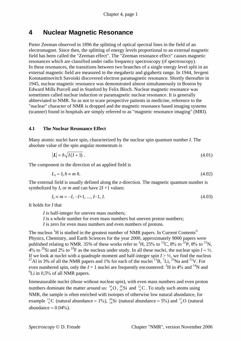
Chapter 4, page 1

4 Nuclear Magnetic Resonance

Pieter Zeeman observed in 1896 the splitting of optical spectral lines in the field of an electromagnet. Since then, the splitting of energy levels proportional to an external magnetic field has been called the "Zeeman effect". The "Zeeman resonance effect" causes magnetic resonances which are classified under radio frequency spectroscopy (rf spectroscopy). In these resonances, the transitions between two branches of a single energy level split in an external magnetic field are measured in the megahertz and gigahertz range. In 1944, Jevgeni Konstantinovitch Savoiski discovered electron paramagnetic resonance. Shortly thereafter in 1945, nuclear magnetic resonance was demonstrated almost simultaneously in Boston by Edward Mills Purcell and in Stanford by Felix Bloch. Nuclear magnetic resonance was sometimes called nuclear induction or paramagnetic nuclear resonance. It is generally abbreviated to NMR. So as not to scare prospective patients in medicine, reference to the "nuclear" character of NMR is dropped and the magnetic resonance based imaging systems (scanner) found in hospitals are simply referred to as "magnetic resonance imaging" (MRI).

4.1 The Nuclear Resonance Effect

Many atomic nuclei have spin, characterized by the nuclear spin quantum number I. The absolute value of the spin angular momentum is

L = +h I I( 1) . (4.01)

The component in the direction of an applied field is

Lz = Iz h ≡ m h. (4.02)

The external field is usually defined along the z-direction. The magnetic quantum number is symbolized by Iz or m and can have 2I +1 values:

Iz ≡ m = −I, −I+1, ..., I−1, I. (4.03)

It holds for I that

I is half-integer for uneven mass numbers; I is a whole number for even mass numbers but uneven proton numbers; I is zero for even mass numbers and even numbers of protons.

The nucleus 1H is studied in the greatest number of NMR papers. In Current Contents© Physics, Chemistry, and Earth Sciences for the year 2000, approximately 9000 papers were published relating to NMR. 35% of these works refer to 1H, 25% to 13C, 8% to 31P, 8% to 15N, 4% to 29Si and 2% to 19F as the nucleus under study. In all these nuclei, the nuclear spin I = ½. If we look at nuclei with a quadruple moment and half-integer spin I > ½, we find the nucleus 27Al in 3% of all the NMR papers and 1% for each of the nuclei 11B, 7Li, 23Na and 51V. For even numbered spin, only the I = 1 nuclei are frequently encountered: 2H in 4% and 14N and 6Li in 0,5% of all NMR papers.

Immeasurable nuclei (those without nuclear spin), with even mass numbers and even proton numbers dominate the matter around us: ,8

16 O 1428 Si and . To study such atoms using

NMR, the sample is often enriched with isotopes of otherwise low natural abundance, for example (natural abundance = 1%), (natural abundance = 5%) and (natural abundance = 0.04%).

612 C

613 C 14

29Si 817 O

Spectroscopy © D. Freude Chapter "NMR", version November 2006

Chapter 4, page 2

The magnetic moment of nuclei can be explained as follows: atomic nuclei carry electric charge. In nuclei with spin, the rotation creates a circular current which produces a magnetic moment µ. An external homogenous magnetic field B results in a torque

T = µ × B (4.04) with a related energy of

E = − µ·B. (4.05) Magnetic quantities are introduced in equ. (2.03). We will use the magnetic induction B written in the units of Tesla (T = Vs m−2) to characterize the magnetic fields instead of the magnetic field strength H in units of A m−1. The magnetization M corresponds to the sum of the magnetic dipole moments µ per unit volume.

The rotation of an electrically charged particle is termed gyration (Greek Gyros = circle). The gyromagnetic (actually magnetogyric) ratio γ, which is important for magnetic resonance, is defined by the equation

µ = γ L. (4.06) The z component of the nuclear magnetic moment, cf. equ. (4.02), is

µz = γ Lz = γ Iz h ≡ γ m h. (4.07) The energy level of a nucleus of nuclear spin I is thereby split in an external field in the z-direction BB0 into 2I + 1 Zeeman levels. The energy difference compared to the state without the magnetic field is

Em = − µz BB0 = − γ mhB0B . (4.08) The macroscopic magnetization, which under the sole influence of an external field aligns itself in the same direction, is M0 = χ0 H0 = χ0 BB0 /µ0, see equ. (2.03). According to definition, it is equal to the sum of the N nuclear moments per unit volume. Using Boltzmann distribution with exp (−Em/kT)/Σmexp(−Em/kt), we can calculate the occupation probability for the level m. From that it follows from the equations (4.07-08) and summation over all values of m that

( )

( )( )M N

m mB kT

mB kT

N I IkT

Bm I

m I

m I

m I0

0

0

2 2

01

3= =

+=−

=+

=−

=+

∑

∑γ

γ

γ

γh

h

h

hexp /

exp /. (4.09)

In the transition from the middle to the right hand side of equ. (4.09), the exponential function was expanded to the linear term. In the summation, use is made of Σm1 = 2I + 1, Σmm = 0 and Σmm2 = I(I + 1)(2I + 1)/3. Because M0 = χ0 H0 = χ0 BB0 /µ0, the quotient multiplied by µ0 on the right hand side of equ. (4.09) represents the statistical nuclear susceptibility. It obeys the Curier law χ0 = C/T, in which the Curier constant C is found using equ. (4.09).

When I = ½, m = ± ½, we get two levels with an energy difference of

ΔE−½,+½ = γ hBB0 = hωL = h νL. (4.10)


Chapter 4, page 3

In equ. (4.10) the energy difference has been replaced by the resonant frequency, which is named after Joseph Larmor, who in 1897 described the precession of orbital magnetization in an external magnetic field. The Larmor frequency νL (or Larmor angular frequency ωL) can be described using a classical model: the torque T acting on a magnetic dipole is defined as the time derivative of the angular momentum L. For this reason, in consideration of equ. (4.06), we get

T L= =

dd

ddt t

1γ

μ. (4.11)

By setting this equal to equ. (4.04), T = µ × B , we see that

ddμ

μt

= ×γ B . (4.12) The summation of all nuclear dipoles in the unit volume gives us the magnetization. For a magnetization that has not aligned itself parallel to the external magnetic field, it is necessary to solve the following equation of motion

ddM M Bt

= ×γ . (4.13)

It is usual to define B = (0, 0, BB0). If we choose M(t = 0) = |M| (sinα, 0, cosα) as initial conditions, the solutions are

Mx = |M| sinα cosωLt, My = |M| sinα sinωLt, (4.14) Mz = |M| cosα.,

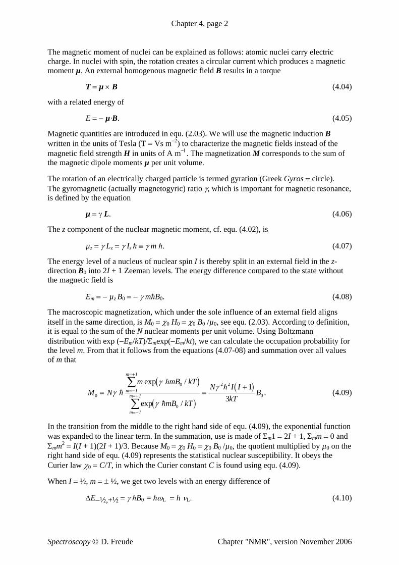
in which ωL = −γBB0 has been used. If the rotation is described by a vector in the direction of the axis of rotation, we have

ωL = −γBB0. (4.15)

B0, z

M

y

x ωL

Fig. 4.1 Larmor precession around the external magnetic field.

The rotation vector is thus opposed to BB0 for positive values of γ. For negative values of γ, both directions are the same. The Larmor relationship is most commonly given as an equation of magnitudes in the form ωL = γB0B or

νγ

L =2 0π

B . (4.16) This most important equation of NMR relates the magnetic field to the resonant frequency. A few values for γ/2π are given in Tab. 4.1. With iron-core and superconductive magnets, modern NMR magnets of 2,4 and 24 Tesla can be built; with those we would get nuclear magnetic resonance frequencies for 1H nuclei of 100 and 1000 MHz, respectively.


Chapter 4, page 4

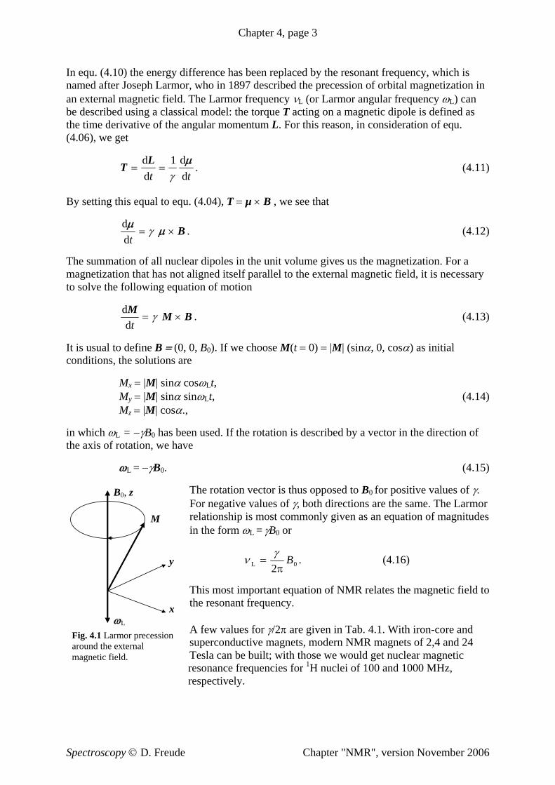
Table 4.1 Gyromagnetic ratio γ/2π in units of MHz/T, nuclear spin and natural abundance of a few nuclei. To get the Larmor frequency νL from γ/2π, we have to multiply with the corresponding value of magnetic induction. A few common values are (νL for 1H is written in parentheses): 2,3488 T (100 MHz), 7,0463 T (300 MHz), 11,7440 T (500 MHz), 17,6157 T (750 MHz), 21,1389 T (900 MHz). 1H 42,58 1/2 99.98% 19F 40.05 1/2 100% 63Cu 11,28 3/2 69,99% 121Sb 10,19 5/2 57,25% 2H 6,535 1 0,015% 23Na 11,42 3/2 100% 65Cu 12,09 3/2 30,91% 127I 8,518 5/2 100% 7Li 16,55 3/2 92,58% 27Al 11,09 5/2 100% 75As 7,291 3/2 100% 133Cs 5,584 7/2 100% 9Be 5,984 3/2 100% 29Si 8,458 1/2 4,7% 77Se 8,118 1/2 7,58% 195Pt 9,153 1/2 33,8% 10B 4,575 3 19,58% 31P 17,24 1/2 100% 79Br 10,67 3/2 50,54% 199Hg 7,590 1/2 16,84% 11B 13,66 3/2 80,42% 35Cl 4,172 3/2 75,53% 81Br 11,50 3/2 49,46% 201Hg 2,809 3/2 13,22% 13C 10,71 1/2 1,108% 37Cl 3,473 3/2 24,47% 87Rb 13,93 3/2 27,85% 203Tl 24,33 1/2 29,5% 14N 3,076 1 99,63% 51V 11,19 7/2 99,76% 93Nb 10,41 9/2 100% 205Tl 24,57 1/2 70,5% 15N 4,314 1/2 0,37% 55Mn 10,50 5/2 100% 117Sn 15,17 1/2 7,61% 207Pb 8,907 1/2 22,6% 17O 5,772 5/2 3,7⋅10−2 59Co 10,05 7/2 100% 119Sn 15,87 1/2 8,58% 209Bi 6,841 9/2 100%

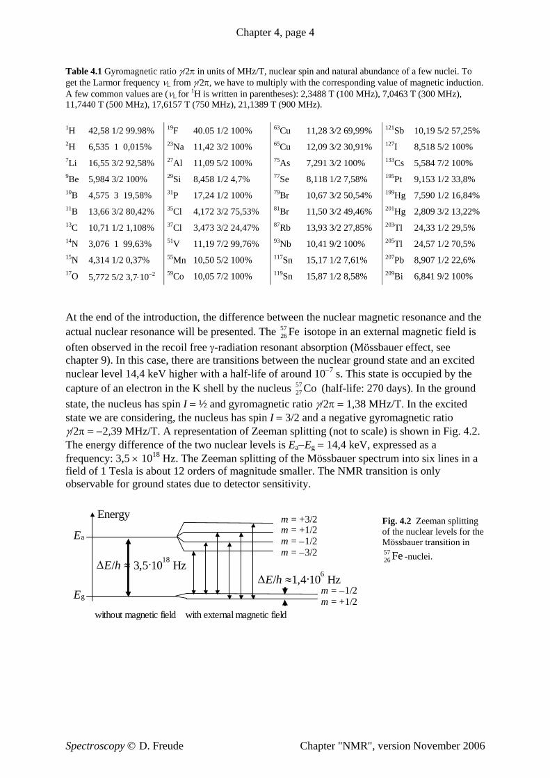
At the end of the introduction, the difference between the nuclear magnetic resonance and the actual nuclear resonance will be presented. The isotope in an external magnetic field is often observed in the recoil free γ-radiation resonant absorption (Mössbauer effect, see chapter 9). In this case, there are transitions between the nuclear ground state and an excited nuclear level 14,4 keV higher with a half-life of around 10

2657 Fe

−7 s. This state is occupied by the capture of an electron in the K shell by the nucleus (half-life: 270 days). In the ground state, the nucleus has spin I = ½ and gyromagnetic ratio γ/2π = 1,38 MHz/T. In the excited state we are considering, the nucleus has spin I = 3/2 and a negative gyromagnetic ratio γ/2π = −2,39 MHz/T. A representation of Zeeman splitting (not to scale) is shown in Fig. 4.2. The energy difference of the two nuclear levels is E

2757 Co

a−Eg = 14,4 keV, expressed as a frequency: 3,5 × 1018 Hz. The Zeeman splitting of the Mössbauer spectrum into six lines in a field of 1 Tesla is about 12 orders of magnitude smaller. The NMR transition is only observable for ground states due to detector sensitivity.

Energy

m = −1/2

m = +1/2 m = +3/2

m = −3/2 m = −1/2

m = +1/2

Ea

Eg

without magnetic field with external magnetic field

ΔE/h ≈1,4·106 HzΔE/h ≈ 3,5·1018 Hz

Fig. 4.2 Zeeman splitting of the nuclear levels for the Mössbauer transition in

-nuclei. 2657 Fe


Chapter 4, page 5

4.2 Basic Set-up of NMR Spectrometers

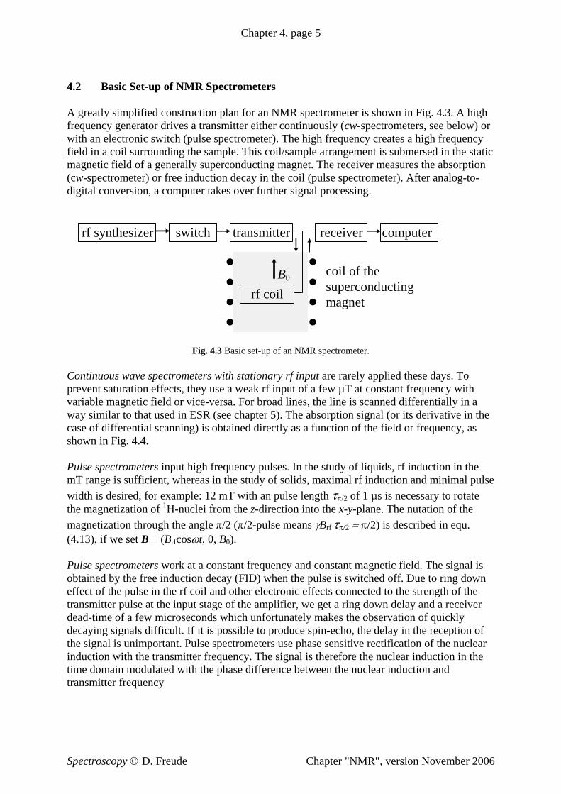
A greatly simplified construction plan for an NMR spectrometer is shown in Fig. 4.3. A high frequency generator drives a transmitter either continuously (cw-spectrometers, see below) or with an electronic switch (pulse spectrometer). The high frequency creates a high frequency field in a coil surrounding the sample. This coil/sample arrangement is submersed in the static magnetic field of a generally superconducting magnet. The receiver measures the absorption (cw-spectrometer) or free induction decay in the coil (pulse spectrometer). After analog-to-digital conversion, a computer takes over further signal processing.

rf synthesizer switch transmitter receiver computer

B0

rf coil

coil of the superconducting magnet

Fig. 4.3 Basic set-up of an NMR spectrometer. Continuous wave spectrometers with stationary rf input are rarely applied these days. To prevent saturation effects, they use a weak rf input of a few µT at constant frequency with variable magnetic field or vice-versa. For broad lines, the line is scanned differentially in a way similar to that used in ESR (see chapter 5). The absorption signal (or its derivative in the case of differential scanning) is obtained directly as a function of the field or frequency, as shown in Fig. 4.4. Pulse spectrometers input high frequency pulses. In the study of liquids, rf induction in the mT range is sufficient, whereas in the study of solids, maximal rf induction and minimal pulse width is desired, for example: 12 mT with an pulse length τπ/2 of 1 µs is necessary to rotate the magnetization of 1H-nuclei from the z-direction into the x-y-plane. The nutation of the magnetization through the angle π/2 (π/2-pulse means γBBrf τπ/2 = π/2) is described in equ. (4.13), if we set B = (BrfB cosωt, 0, BB0). Pulse spectrometers work at a constant frequency and constant magnetic field. The signal is obtained by the free induction decay (FID) when the pulse is switched off. Due to ring down effect of the pulse in the rf coil and other electronic effects connected to the strength of the transmitter pulse at the input stage of the amplifier, we get a ring down delay and a receiver dead-time of a few microseconds which unfortunately makes the observation of quickly decaying signals difficult. If it is possible to produce spin-echo, the delay in the reception of the signal is unimportant. Pulse spectrometers use phase sensitive rectification of the nuclear induction with the transmitter frequency. The signal is therefore the nuclear induction in the time domain modulated with the phase difference between the nuclear induction and transmitter frequency


Chapter 4, page 6

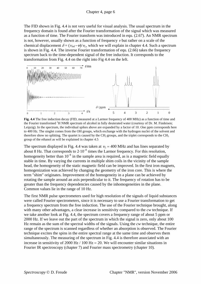
The FID shown in Fig. 4.4 is not very useful for visual analysis. The usual spectrum in the frequency domain is found after the Fourier transformation of the signal which was measured as a function of time. The Fourier transform was introduced in equ. (2.67). An NMR spectrum is not, however, usually shown as a function of frequency ν but rather on a scale of the chemical displacement δ = (νref −ν)/νL, which we will explain in chapter 4.4. Such a spectrum is shown in Fig. 4.4. The inverse Fourier transformation of equ. (2.66) takes the frequency spectrum back to the time-dependent signal of the free induction. It corresponds to the transformation from Fig. 4.4 on the right into Fig 4.4 on the left.

1 2 3 4 0

10 20 30 40 50 60 70 0 t/ms

t/s

0 1 2 3 4 5

δ / p p m

Fig. 4.4 The free induction decay (FID, measured at a Larmor frequency of 400 MHz) as a function of time and the Fourier transformed 1H NMR spectrum of alcohol in fully deuterated water (courtesy of Dr. M. Findeisen; Leipzig). In the spectrum, the individual spikes above are expanded by a factor of 10. One ppm corresponds here to 400 Hz. The singlet comes from the OH groups, which exchange with the hydrogen nuclei of the solvent and therefore show no splitting. The quartet is caused by the CH2 groups, and the triplet corresponds to the CH3 group of the ethanol as will be explained in chapter 4.5

The spectrum displayed in Fig. 4.4 was taken at νL = 400 MHz and has lines separated by about 8 Hz. That corresponds to 2⋅10−8 times the Larmor frequency. For this resolution, homogeneity better than 10−8 in the sample area is required, as is a magnetic field equally stable in time. By varying the currents in multiple shim coils in the vicinity of the sample head, the homogeneity of the static magnetic field can be improved. In the first iron magnets, homogenization was achieved by changing the geometry of the iron core. This is where the term "shim" originates. Improvement of the homogeneity in a plane can be achieved by rotating the sample around an axis perpendicular to it. The frequency of rotation has to be greater than the frequency dependencies caused by the inhomogeneities in the plane. Common values lie in the range of 10 Hz.

The first NMR pulse spectrometers used for high resolution of the signals of liquid substances were called Fourier spectrometers, since it is necessary to use a Fourier transformation to get a frequency spectrum from the free induction. The use of the Fourier technique brought, along with many other advantages, a clear increase in sensitivity compared to the cw technique. If we take another look at Fig. 4.4, the spectrum covers a frequency range of about 5 ppm or 2000 Hz. If we leave out the part of the spectrum in which the signal is zero, only about 100 Hz remain as the sum of the spectral widths of the signals. Using the cw technique, the entire range of the spectrum is scanned regardless of whether an absorption is observed. The Fourier technique excites the spins in the entire spectral range at the same time and observes them simultaneously. The measuring of the spectrum in Fig. 4.4 is therefore associated with an increase in sensitivity of 2000 Hz / 100 Hz = 20. We will encounter similar situations in Fourier IR spectroscopy (chapter 7) and Fourier mass spectrometry (chapter 10).


Chapter 4, page 7

4.3 Nuclear Magnetic Relaxation Time and Measurement Sensitivity

Spectra are represented as functions of frequency or frequency shift. In contrast, relaxation times describe the time dependency of the generation or decay of certain orders. Many relaxation times are difficult or impossible to measure with cw Spectrometers. We will, however, show that in transversal relaxation, the relaxation time determined by the free induction decay is related to the line width of the frequency spectrum. The study of nuclear magnetic relaxation has achieved certain independence in the study of dynamic processes, so that it is sometimes separated from the study of nuclear magnetic resonance. Nuclear magnetic relaxation is related to nuclear resonance, but it cannot be portrayed in a single nuclear resonance spectrum. Instead of one spectrum, the dependency of a relaxation time on the measurement frequency or observation temperature is plotted. The fundamental relaxation time of NMR is the longitudinal relaxation time T1 that well be explained now.

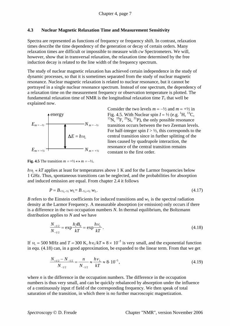
Consider the two levels m = −½ and m = +½ in Fig. 4.5. With Nuclear spin I = ½ (e.g. 1H, 13C, 15N, 19F, 29Si, 31P), the only possible resonance transition occurs between the two Zeeman levels. For half-integer spin I > ½, this corresponds to the central transition since in further splitting of the lines caused by quadrupole interaction, the resonance of the central transition remains constant to the first order.

energy

Em = −½

Em = +½

N m = −½

N m = +½

ΔE = hνL

Fig. 4.5 The transition m = +½ ↔ m = −½.

hνL « kT applies at least for temperatures above 1 K and for the Larmor frequencies below 1 GHz. Thus, spontaneous transitions can be neglected, and the probabilities for absorption and induced emission are equal. From chapter 2.4 it follows

P = BB+½,−½ wL= B−½,+½B wL. (4.17) B refers to the Einstein coefficients for induced transitions and wL is the spectral radiation density at the Larmor Frequency. A measurable absorption (or emission) only occurs if there is a difference in the two occupation numbers N. In thermal equilibrium, the Boltzmann distribution applies to N and we have

NN

BkT

hkT

+

−

= =1 2

1 2

0/

/

exp exphγ νL . (4.18)

If νL = 500 MHz and T = 300 K, hνL/kT ≈ 8 × 10−5 is very small, and the exponential function in equ. (4.18) can, in a good approximation, be expanded to the linear term. From that we get

N NN

nN

hkT

+ −

− −

−−= ≈ ≈ ⋅1 2 1 2

1 2 1 2

58 10/ /

/ /

ν L , (4.19)

where n is the difference in the occupation numbers. The difference in the occupation numbers is thus very small, and can be quickly rebalanced by absorption under the influence of a continuously input rf field of the corresponding frequency. We then speak of total saturation of the transition, in which there is no further macroscopic magnetization.


Chapter 4, page 8

On the other hand, since we see that in equ. (4.18) that as the temperature tends toward infinity, the difference between the occupation numbers tends to zero, we can use the difference in the occupation numbers to define a spin temperature. This "temperature" is not necessarily the same as the surrounding temperature. An inversion of the occupation numbers corresponds to a change of sign of the temperature, and the balancing of the occupation numbers leads to an infinite temperature of the spin system. All degrees of freedom of the system except for the spin (e.g. nuclear oscillations, rotations, translations, external fields) are called the lattice. Setting thermal equilibrium with this lattice can be done only through induced emission. The fluctuating fields in the material always have a finite frequency component at the Larmor frequency (though possibly extremely small), so that energy from the spin system can be passed to the lattice. The time development of the setting of equilibrium can be described after either switching off or on the external field BB0 at time t = 0 (difficult to do in practice) with

10

Tt

enn−

= or ⎟⎟⎠

⎞⎜⎜⎝

⎛−=

−

110T

t

enn , (4.20)

respectively. T1 is the longitudinal or spin-lattice relaxation time an n0 denotes the difference in the occupation numbers in the thermal equilibrium, if the external field is on. Longitudinal relaxation time because the magnetization orients itself parallel to the external magnetic field corresponding to the difference in the occupation of the two levels. The relation between the longitudinal relaxation time T1 and the transition probability P in a two level system is

1/T1 = 2P = 2BB−½,+½ wL, (4.21) which follows from

( )dd

dd

Nt

P N N Pn nT

nt

++ −= − − = − = − =1 2

1 2 1 21

12

12

// / , (4.22)

where we used N+½ = ½ {(N+½+N−½) + n} and dn/dt = −n/T1 from equ. (4.20). The difference in the occupation numbers n is proportional to BB0 and depends on the temperature T in accordance with equations (4.18-19). The dependency of T1 on the value of the spectral density function at the resonant frequency ωL has to be discussed in detail for special interactions, as will be done below for a homo-nuclear two spin system. In the introduction of equ. (4.20), we assumed at the right an activation of the external field at time t = 0. In practice, the value of T1 in the simplest case is measured with the aid of two pulses. In chapter 4.2 we described the π/2-pulse, which rotates a macroscopic magnetization in thermal equilibrium oriented parallel to the external magnetic field (z-direction) into the x-y-plane. After the π/2- pulse there is no further magnetization in the z-direction, which, in the picture above (Fig. 4.5), corresponds to the disappearance of the difference in occupation numbers. Instead of a difference in population, which cannot be directly observed by NMR methods, we have an observable "coherence". The term "coherence" is used because the phases of all rotating nuclear spins are the same as the phase of the incoming high frequency through the strong high frequency field. With that, after the pulse, the rotation of the macroscopic magnetization into the x-y-plane can be observed in the signal induced in the coil. This free induction (FID) or phase coherence of the spin decays with the transversal relaxation time T2, which is yet to be discussed.


Chapter 4, page 9

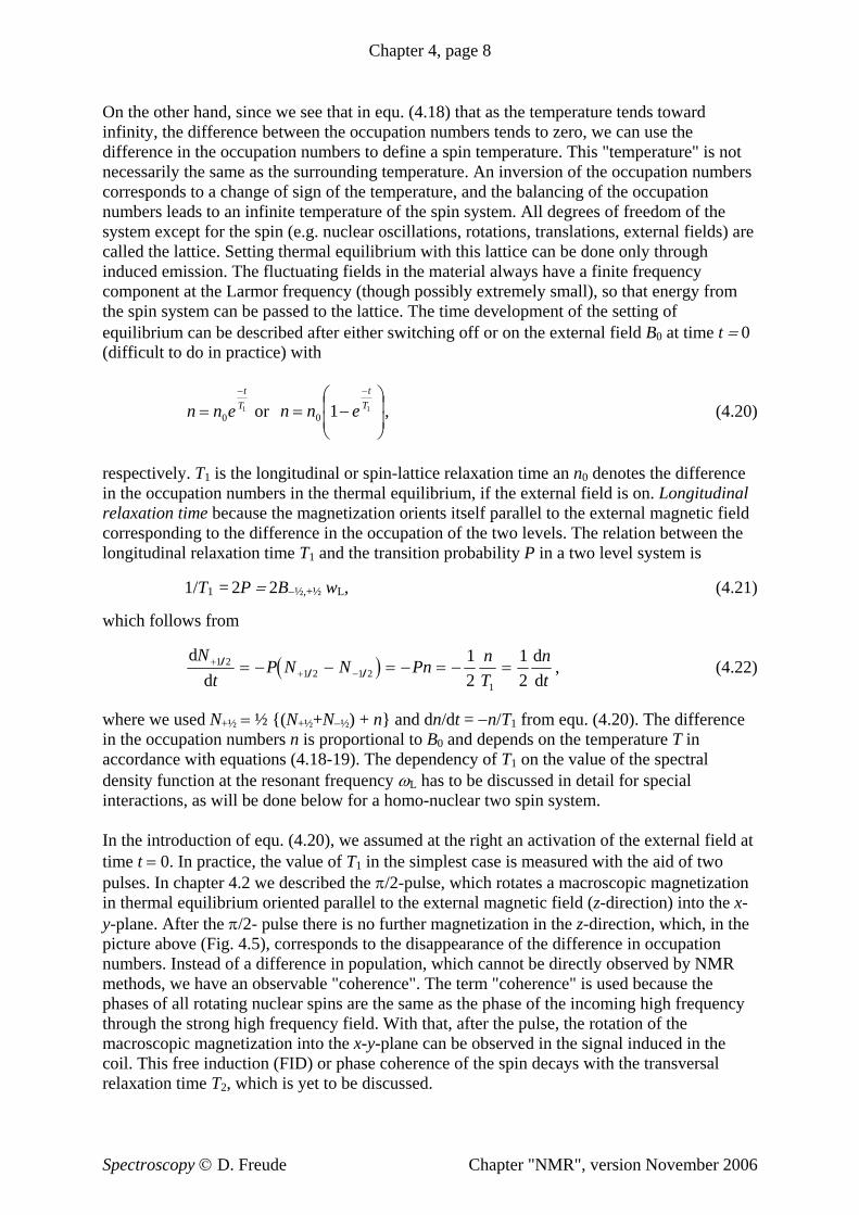
We will now consider the action of a π pulse, which has twice the length of a π/2 pulse, i.e. for a pulse length τπ, it holds that γBBrfτπ = π. An pulse of this type rotates the magnetization from the z-direction to its opposite, the −z-direction. In our picture, this corresponds to an inversion of the occupation numbers. If we consider the equations (4.18-19), this inversion of the populations can be described by a reversal of the sign of the temperature. Through the action of the π pulse, we create an equally large but "negative" temperature of the spin system. In this physically questionable though very useful "temperature" picture, the Boltzmann equation for thermal equilibrium is applied to a state not in thermal equilibrium. With the π pulse, the population differences which are non-observable with NMR are reversed. Since no observable coherences are created, we still need a further π/2 pulse to measure the T1-relaxation after the π pulse (adjustment of the temperature of the spin system to the positive temperature of the lattice). This pulse has the already mentioned property that the population differences are converted into observable coherences. Taking phase relationships into consideration, the application of a π/2 pulse directly after a π pulse results in a negative signal. This signal has the same magnitude as the positive signal that would have been created had we used a π/2 pulse alone. With increasing pulse delay τ , the negative signal corresponding to the T1 relaxation of the spin system is reduced. After time τ0 the signal goes through zero since no further macroscopic population differences are observable. This corresponds to the transition from a negative spin temperature through "finite" to a positive spin temperature. As the time τ further increases, the now positive signal approaches the value that would have been observed after the sole application of a π/2 pulse. A similar experiment can be described by two π/2 pulse using equ. (4.20). The time development of the π-π/2 experiment (inversion recovery experiment) of Fig. 4.6 obeys the equation

⎟⎟⎠

⎞⎜⎜⎝

⎛−=

−

121mequilibriu thermalTennτ

. (4.23)

By setting the parentheses in equ. (4.23) equal to zero, we get τ0 = T1 ln2 as the passage of zero. From that we have a simple procedure to determine T1, which, however, requires good adjustment of the pulse lengths and a homogenous high frequency field.

Fig. 4.6 The inversion recovery experiment for the determination of T1.


Chapter 4, page 10

As an example for the calculation of relaxation times, we consider a homo-nuclear two spin system (nuclear separation r) of a molecule in a liquid. We will neglect intermolecular nuclear magnetic interaction. Every spin is affected by the external magnetic field, which is superimposed with the z-component of the dipole-dipole interaction of neighboring atoms (this fluctuates due to molecular motion). A time-(t)-independent correlation function G(τ) of a function f(t) describes the magnetic interaction:

( ) ( ) ( )G f t f tτ = + τ . (4.24)

The pointy brackets in equ. (4.24) refer to the ensemble average over all particles. In chapter 8 of the classic NMR textbook of A. Abragam, it is shown that in the special case of rotational diffusion an exponential approach applies to a good approximation, from which the correlation time τc is defined:

( ) ( )G Gc

τττ

= −⎛

⎝⎜

⎞

⎠⎟0 exp . (4.25)

If you imagine, for example, that a large molecule is reoriented by collisions with neighboring molecules, τc is approximately the average time in which the molecule has reoriented itself through the solid angle 1. With the approach of (4.25), we get for T1 (see Abragam, p. 300)

( )( ) ( ) ⎟⎟

⎠

⎞⎜⎜⎝

⎛

++

++⎟

⎠⎞

⎜⎝⎛= 2

L2

L

20

6

24

1 218

121

4511

c

c

c

cIIrT τω

ττω

τπ

μγ h (4.26)

and for the transversal relaxation time T2

( )( ) ( ) ⎟

⎟⎠

⎞⎜⎜⎝

⎛

++

+++⎟

⎠⎞

⎜⎝⎛= 2

L2

L

20

6

24

2 212

15

3145

11

c

c

c

ccII

rT τωτ

τωτ

τπ

μγ h . (4.27)

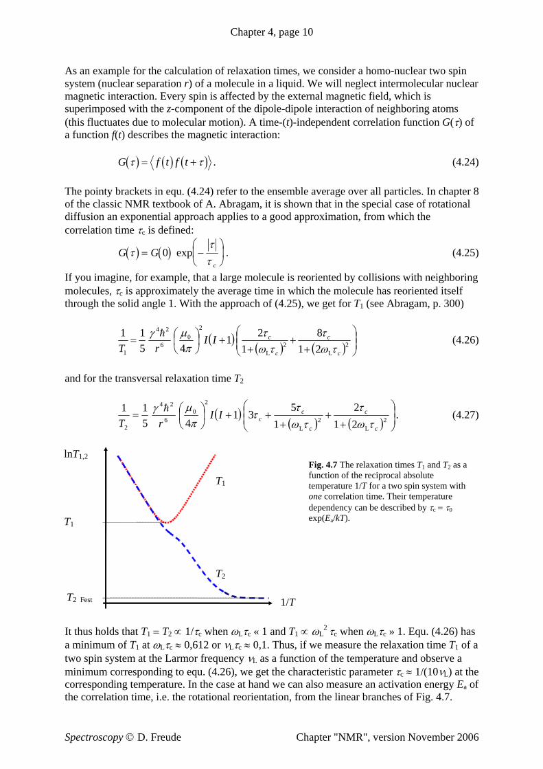
Fig. 4.7 The relaxation times T1 and T2 as a nction of the reciprocal absolute

thus holds that T1 = T2 ∝ 1/τc when ωLτc « 1 and T1 ∝ ωL2 τc when ωLτc » 1. Equ. (4.26) has

minimum of T at ω τc ≈ 0,612 or ν τc ≈ 0,1. Thus, if we measure the relaxation time T of a

of

T1

T2

lnT1,2

1/T

T1

T2 Fest

futemperature 1/T for a two spin system with one correlation time. Their temperature dependency can be described by τc = τ0 exp(Ea/kT).

Ita 1 L L 1

two spin system at the Larmor frequency νL as a function of the temperature and observe a minimum corresponding to equ. (4.26), we get the characteristic parameter τc ≈ 1/(10νL) at the corresponding temperature. In the case at hand we can also measure an activation energy Eathe correlation time, i.e. the rotational reorientation, from the linear branches of Fig. 4.7.


Chapter 4, page 11

If we have to consider anisotropic rotational diffusion or multiple correlation times in the haracterization of a system, or if we can’t use an exponential function for the temperature c

dependency, then the temperature development of the relaxation times in a liquid gets mucmore complicated. In Fig. 4.7, T

h

ime is relaxation. We will start with a phenomenological

T2

y

2 becomes a constant at low temperatures (dotted line). Thisresults from the fact that equ. (4.27) only applies if τc < T2. If τc surpasses the value given byequ. (4.27), we see behavior resembling that of a solid body in the NMR spectrum, with a temperature independent value of T2.

Since we have already discussed the temperature dependency of the transversal relaxation tT2, we will now explain the cause of thexplanation of relaxation effects which assume that the reconstruction of a magnetization differing from static equilibrium in the z-direction is described by the relaxation time T1, anddescribes the decay of the transversal component of the magnetization in the x-y-plane.

To derive the equations introduced by Felix Bloch into nuclear resonance (and later also into on-linear optics), we add two relaxation terms to equ. (4.13) and take the high frequencn

field BB

d high

rf into account. We get into the so-called "rotating" coordinate system, which rotates with the angular frequency ω around the z axis of the laboratory coordinate system. The direction of rotation is mathematically positive when the gyromagnetic ratio γ is negative annegative if the ratio is positive. The unit vectors of the rotating system are ex, ey, ez. The frequency field is input with a coil in the x-direction of the laboratory coordinate system with the frequency ω and amplitude 2BrfB . This linear polarized field can be described by two circular polarized fields which rotate with the frequency ω in the positive and negative sense around the z axis. From that we get an x-component BB rf in the rotating coordinate systemwhich is time-independent at stationary input of high frequency (cw input). Instead of the external magnetic field, the only action in the rotating coordinate system is the magnetic induction of the resonance deviation (ωL−ω)/γ, the "offset" or "resonant offset". If for the spins under study the input high frequency is identical to the Larmor frequency ωL = |γ|B0offset disappears. The effective working field in the rotating coordinate system is a vector addition of the rf field and the offset Beff

B , the

B = (BBrf, 0, B0B (4.28)

ith that w

−ω /γ). W e get the Bloch equations

( )1

0

2eff

d M xxeBMM

d TMM

TM

tz zyy ee −

−+

−×= γ . (4.29)

0 is the equilibrium magnetization introduced in equ. (4.09),tarting condition after the switching off of the rf field and the dying out of the T1-relaxation

ey

M which adjusts itself for any sin the z-direction. Stationary solutions to the Bloch equations are attained for dM/dt = 0. Thare

( )( )

( )( )

( ).

11

,21

,21

021

2rf

222

2L

22

2L

rf0rf21

2rf

222

2L

2

rf0rf21

2rf

222

2L

2Tωω − 2L

MTTBT

TM

HMBTTBT

TM

HMBTTBT

M

z

y

x

γωωωω

χγγωω

χγγωω

+−+−+

=

′′=+−+

=

′=+−+

=

(4.30)


Chapter 4, page 12

χ = χ' − iχ" was introduced as the complex susceptibility of the high frequency field. In the cw-procedure, a weak rf field is usually used to prevent saturation. The conditions for this are

γ2Brf2 T1T2 « 1.

no saturation) the solutions of the Bloch equations simMz = M0 = χ0H0, see equ. (4.10). χ' and χ" no longer depend on the rf field.

The power absorbed by the spin system is the value averaged over one period of rotation in t

(4.31)

In this case ( plify considerably, e.g.

he laboratory coordinate system. It can be electronically measured in the sample coil.

t

Pd

d rfBM= (4.32) −

The rf field is linearly polarized there and only has an x component 2BBrf cosωt, whose time derivative is −2ωBrfB nt of M. After sinωt. We are therefore only interested in the x componetransformation into the laboratory coordinate system we get

Mx(t) = 2BB (4.33) −MxdBrf/dt 2ω

rf(χ'cosωt + χ"sinωt)/µ0.

In the product only the term with sin t remains after averaging over the period of rotation, which, when averaged over time, has a value of ½. The absorbed power is

P = 2 ωLBB 4)

rm of the free induction),

.30)

rf2 χ"/µ0. (4.3

It can be seen in equ. (4.34) that the line form of the absorption signal, which was measured as absorbed power over input frequency (or as Fourier transfodepends on the imaginary part of the susceptibility. Due to the weak rf input, we get from equ. 4(

( )

′′ =+ −

χω ω

γ μ12

221 2L

2T(4.35)

0 0T M .

This gives us a Lorentz line form, which we recognize from equ. (2.71) or Fig. 2.5 in chapter2.6. It is typical in NMR for spin systems influenced by motion. The half-width δν½ is called the full width at half maximum (fwhm), and is shown in Fig. 2.5. From equ. (4.35) we get

δνπ1 2

2

1/ =

T, (4.36)

om which the transversal relaxation time ise lines that gave T1 the name spin-lattice relaxation time, T2 is called the spin-

a eld B , so that the re

fr brought into connection with the line width. Along the samspin relaxation time. For example, in a solid body, the dipole-dipole interaction between two nuclear spins is the most important cause of line broadening for nuclei where I = ½. At the location of the nucleus under consideration, the dipoles of neighboring nuclei create an extr

Local Localfi sonance frequency of the nucleus is ν = (BB0+BzB

onsider the homo-nucleetween r and e , then we get

) γ/2π. If we again c ar two spin system with the inter-atomic distance r and the angle θ b z

Δω γ μπ

θ= ±

−32 4

3 12

2

30

2I h

rcos (4.37

for the resonance shift caused by the dipolar interaction in the solid body where m = ±½ is thestate of the neighboring spin.

)


Chapter 4, page 13

In powder samples, the orientations of the inter-atomic vectors to the external magnetic fieldare statistically distributed. The 2

−

term 3cos θ −1 in equ. (4.37) assumes values between 2

nd 1. Thus a broadening of the resonance line occurs. In liquids, through the rapid orientation of the inter-atomic vectors

arrowing is inverse proportion to τc (exrom equations (4.34-36) it can be immediately seen that as the line is narrowing (extension

A narrowing of the solid body signal can be reached by rapid rotation of the sample around the magic-angle (magic-angle spinning, MAS). For the magic-angle arccos 3−1/2 ≈ 54,74° the geometry dependent factor in equ. (4.37) becomes zero, i.e. a dipole-dipole interaction at this angle to the external magnetic field does not cause resonant shifting. It is now necessary to average out the dipole-dipole interactions perpendicular to this direction. This is accomplished by rapid rotation of the sample around an axis that includes the magic-angle with the external magnetic field. We can thereby drastically reduce the dipole-dipole broadening of a solid body signal, if the rotation frequency is greater than the width of the spectra given by equ. (4.37). The air beard and driven rotors have frequencies between 1 and 60 kHz.

Beside the homo-nuclear dipole-dipole interaction, there are other causes which lead to resonance shifting with the geometry factor 3cos2θ −1: heteronuclear interaction, anisotropy of the chemical shift (see chapter 4.4), and quadrupole interaction (the nuclear quadrupole moment for I < ½ with the electric field gradient tensor with respect to the first order). The broadening of the signals of powder samples as a consequence of these interactions can also be averaged out by means of MAS. Besides the increase in detection sensitivity resulting from the narrowing of lines, a more exact determination of the resonant frequency and the value of the chemical shift is obtained, see chapter 4.4. Rapid sample rotation has become a fundamental technology in solid-state NMR.

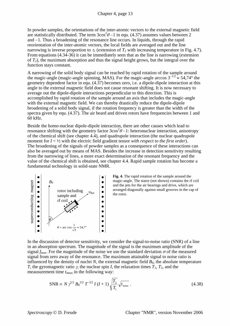
Fig. 4. The rapid rotation of the sample around the magic-angle. The stator (not shown) contains the rf coil and the jets for the air bearings and drive, which are arranged diagonally against small grooves in the cap of the rotor.

In the discussion of detector sensitivity, we consider the signal-to-noise ratio (SNR) of a line in an absorption spectrum. The magnitude of the signal is the maximum amplitude of the signal fmax. For the magnitude of the noise we use the standard deviation σ of the measured signal from zero away of the resonance. The maximum attainable signal to noise ratio is influenced by the density of nuclei N, the external magnetic field B0, the absolute temperature T, the gyromagnetic ratio γ, the nuclear spin I, the relaxation times T1, T2, and the meausurement time tmeas in the following way:

SNR ∝ N γ5/2 B03/2 T−3/2 I (I + 1)

are , the local fields are averaged out and the line n tension of T2 with increasing temperature in Fig. 4.7). Fof T2), the maximum absorption and thus the signal height grows, but the integral over the function stays constant.

θ

B0

νRot rotor including sample and rf coil

θ = ≈arc ocos ,13

54 7

supe

rcon

duct

ing

mag

net

meas1

2 tTT . (4.38)


Chapter 4, page 14

The proportionality to N is due to the fact that the magnetization is the sum of nuclear moments per unit volume. The equ. (4.09) in chapter 4.1 (equilibrium magnetization) contthe factors I(I+1)γ

ains 2 BB power 0

1 T . In the derivation of equ. (4.34) we see that the measurable in the rf coil is proportional to ω

−1

L, from which follows an additional proportionality of the SNR to γ B0

1B

1. The frequency and temperature dependence of the electronic noise is give by ωT (white noise per definition). From that we get the extra factors γ−1/2 BB

owers of γ, B0 and T in equ. (4.38).

he

measT T t n

0−1/2 T in the

SNR. This explains the p

−1/2

The detection of nuclear resonances is always done by the observation of one component of the macroscopic magnetization in the x-y-plane (preferably after a π/2 pulse). This componentrotates around the z-axis at the Larmor frequency and can be observed as induction in the coil in the x-direction before it decays after a time on the order of the transversal relaxation timeT2. If we want to conduct a new NMR experiment afterwards, we have to wait for a time onthe order of the longitudinal relaxation time T1, before the macroscopic magnetization has returned to its equilibrium state in the z-direction. We could then apply a π/2 pulse, watch tfree induction, and add the new signal to the one we already have in the computer. This signalaccumulation process is continually repeated during the measurement period t of a few minutes to days. The sum of the effective observation time is then ( 2/ 1) meas. The number of statistically independent measurement points increases in proportion to the effective observation time. The signal is overlaid with a normal distribution error by the electronic noise. From error calculations it is known that the average value of n measurements only differs on average from the true value by

Δxn

=σ . (4.39)

The factors

T T2 1 meast in equ. (4.38) are thus explained. With n signal accumulations where n = tmeas/T1, these factors can be replaced w nTith 2 , whereby the dependency on the

which only depends on the location of the ifferent n

number of scans can be better demonstrated.

In equ. (4.38), γ5/2I(I+1) represents a quantitynuclei. It tells us the "relative sensitivity" of d uclei in the same field. If we set the numerical value to 1 for 1H, then, using the same number of nuclei used in 1H, and with the same field strength (but naturally different Larmor frequencies), we get a measurement sensitivity of 0,016 for 13C, 10−3 for 15N, 0,83 for 19F, 0,1 for 23Na, 0,2 for 27Al and 0,01 for 29Si. More exact numerical values for these and other nuclei can be calculated from the values in Tab. 4.1. The value given here for 13C is further reduced if we have to make do with the natural abundance of 13C nuclei (1,11%). Despite this sensitivity disadvantage, this nucleus is studied

ations ssible for the quotient T1 /T2 to assume values

up to 108. This results in etection sensitivity of up to 10−4 times, as calculated from

almost as often as the 1H nucleus. It is caused on the one hand by the central role of carbon in chemistry and on the other hand by the more simple spectrum, since the number of carbonatoms is mostly smaller than the number of hydrogen atoms in organic compounds. Before we move on to the section on chemical shifts, we want to clarify a difference between solid-state and liquid NMR. T1/T2 is about one for liquids, as can be seen in the equ4.26-27) when ωLτc<<1. In solid bodies, it is po(

a reduced dequ. (4.38).


Chapter 4, page 15

4.4 Chemical Shift

The external magnetic field BB

the nu is l o e s bi

rnal field. If the valence

0 can only affect a nucleus without shielding, if the atom has been stripped of its electrons. Through the action of the electron shell, the magnetic field at

cleus is changed. This can be understood by imagining that, when the magnetic field turned on, an opposing current is induced in the spherical electron shel f th or tal. Thisroduces an extra (diamagnetic) field which opposed the extep

electrons are not in the spherically symmetric p orbitals, then the external field affects the electron shell in such a way that a field proportional and co-directional to the external field is created, thus resulting in paramagnetic shift. The resulting field BB0' at the nucleus is described by a shielding constant σ ( )′ = −B B0 01 σ . (4. The charge distribution of the bonding electrons is affected by the chemical bonds. For this reason, the effect of the shift of the nuclear magnetic resonance is called the chemical shift. The shielding constant σ is only still used in theoretical considerations. The reason is that the resonance frequency of the bare nucleus is not appropriate as a point of reference, becauseis not experimentally measurable. Instead of that, an easily measurable reference substanceused to define the dimensionless value, usually given in parts per million (ppm, 10 ), of tchemical shift δ

40)

it is

he −6

σ− . (4.41) σδ = Reference

gn is changed: A positive chemical shift δ

teristic isotropic screening or isotropic chemical shift given by the trace of the

ical

can be tested against the measured values of the screening constant.

Reference substances are usually standard by convention, e.g. TMS (tetramethylsilane, Si(CH3)4) for the three nuclei 1H, 13C and 29Si NMR. Take note that when using the chemical shift δ instead of magnetic screening σ , the siindicates less screening and a correspondingly higher resonance frequency at the same external field B0. The distribution of the electron density is not, in general, isotropic. For this reason, both screening and chemical shift are tensors by nature. In NMR studies on solids, it is possible to measure different screening along the main axes of the bonding system. In liquids, molecular units reorient themselves so quickly that only the average value of the screening is observable, i.e. the characscreening tensor. In the 1H NMR, the diamagnetic contributions of the screening dominate. In other nuclei, paramagnetic contributions can take precedence. If multiple bonds occur in the vicinity, separation into diamagnetic and paramagnetic components is questionable. Classical calculations can, at best, describe a diamagnetic shift. Semi-empirical quantum chemcalculations of screening are not free of random assumptions, so that the ab initio calculation of quantum chemistry is often used to calculate the chemical shift. Due to the enormous amount of experimental data for chemical shifts, it is rarely necessary to use calculated values for the interpretation of spectra. Nevertheless, the calculation of chemical shifts has remained a fundamental problem in theoretical works. On the other hand, quantum mechanical calculations


Chapter 4, page 16

The size of the δ scale covered by the individual nuclei in different molecules increases with ei, about 20 ppm of the δ scale is covered, in 13C about 400 ppm,

and in 205Tl about 10 000 ppm. The chemical shifts of nuclei in liquid substances have been of

over up

e of the OH protons with the protons of the solvent water, whose hemical shift is 4,78 ppm. Due to a small residual concentration of H2O in the solvent D2O, e relative intensity of thee CH2 and CH3 groups by scalar coupling will be explained in chapter 4.5.

f

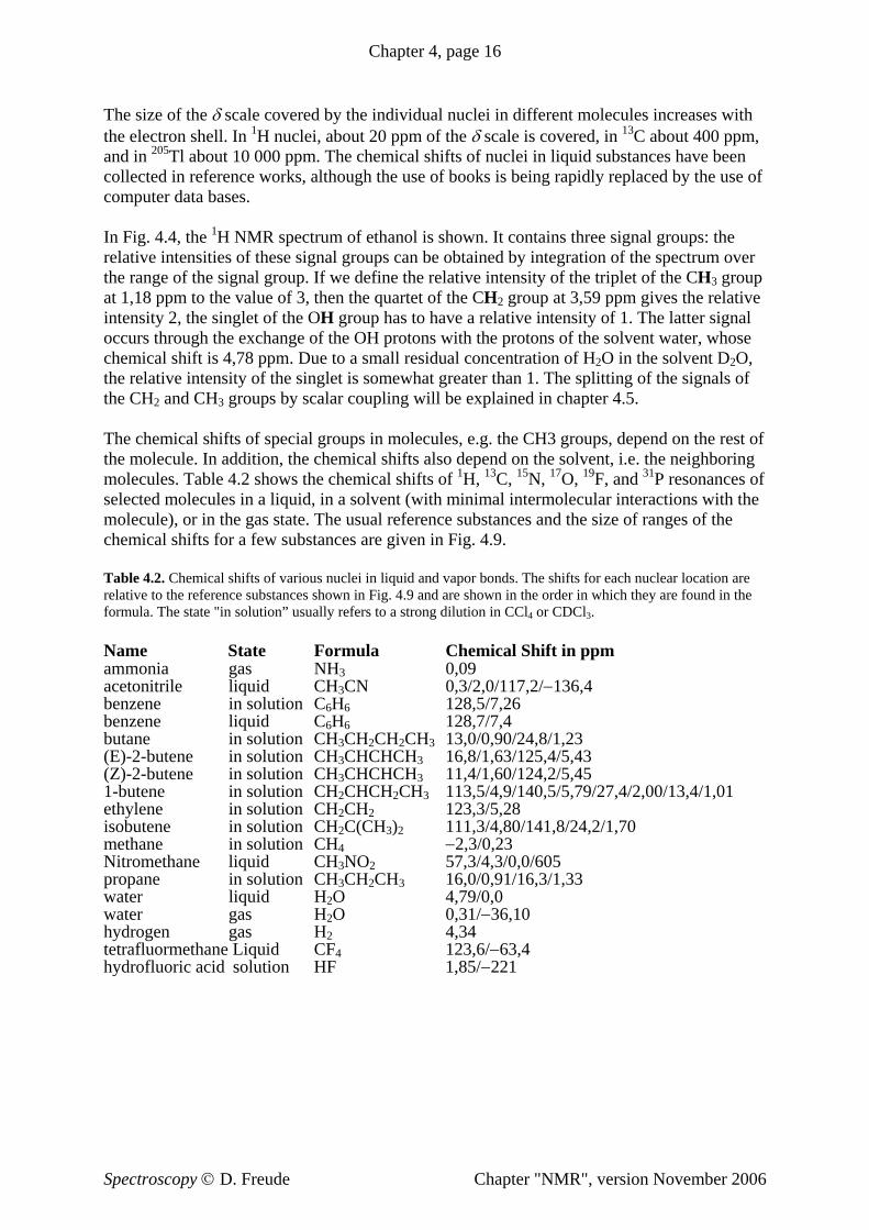
able 4.2. Chemical shifts of varilative to the reference substancermula. The state "in solution” usually refers to a strong dilution in CCl4 or CDCl3.

liquid C6H6 128,7/7,4 utane in solution CH CH CH CH 13,0/0,90/24,8/1,23

quid CH3NO2 57,3/4,3/0,0/605 ropane in solution CH3CH2CH3 16,0/0,91/16,3/1,33

the electron shell. In 1H nucl

collected in reference works, although the use of books is being rapidly replaced by the usecomputer data bases. In Fig. 4.4, the 1H NMR spectrum of ethanol is shown. It contains three signal groups: the relative intensities of these signal groups can be obtained by integration of the spectrumthe range of the signal group. If we define the relative intensity of the triplet of the CH groat 1,18 ppm to the value of 3, then the quartet of the CH group at 3,59 ppm gives the relative intensity 2, the singlet of the OH group has to have a relative intensity of 1. The latter signal occurs through the exchang

3

2

cth singlet is somewhat greater than 1. The splitting of the signals of th The chemical shifts of special groups in molecules, e.g. the CH3 groups, depend on the rest othe molecule. In addition, the chemical shifts also depend on the solvent, i.e. the neighboring molecules. Table 4.2 shows the chemical shifts of 1H, 13C, 15N, 17O, 19F, and 31P resonances ofselected molecules in a liquid, in a solvent (with minimal intermolecular interactions with the molecule), or in the gas state. The usual reference substances and the size of ranges of the chemical shifts for a few substances are given in Fig. 4.9. T ous nuclei in liquid and vapor bonds. The shifts for each nuclear location are re s shown in Fig. 4.9 and are shown in the order in which they are found in the fo Name State Formula Chemical Shift in ppm ammonia gas NH3 0,09 acetonitrile liquid CH3CN 0,3/2,0/117,2/−136,4 benzene in solution C6H6 128,5/7,26 benzene b 3 2 2 3(E)-2-butene in solution CH3CHCHCH3 16,8/1,63/125,4/5,43 (Z)-2-butene in solution CH3CHCHCH3 11,4/1,60/124,2/5,45 1-butene in solution CH2CHCH2CH3 113,5/4,9/140,5/5,79/27,4/2,00/13,4/1,01 ethylene in solution CH2CH2 123,3/5,28 isobutene in solution CH2C(CH3)2 111,3/4,80/141,8/24,2/1,70 methane in solution CH4 −2,3/0,23 Nitromethane lipwater liquid H2O 4,79/0,0 water gas H2O 0,31/−36,10 hydrogen gas H2 4,34 tetrafluormethane Liquid CF4 123,6/−63,4 hydrofluoric acid solution HF 1,85/−221


Chapter 4, page 17

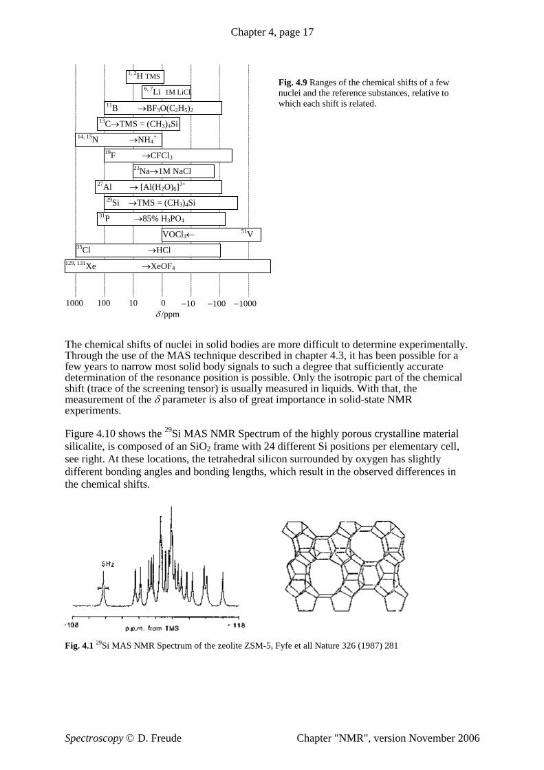
Fig. 4.9 Ranges of the chemical shifts of a few nuclei and the reference substances, relative to which each shift is related.

ult to determine experimentally.

that, the ent of the eter is als great im

stalline material elementary cell,

n has slightly d differences in

he chemical shifts of nuclei in solid bodies are more diffic

1, 2H TMS 6, 7Li 1M LiCl

11B →BF3O(C2H5)2 13C→TMS = (CH3)4Si

14, 15 +N →NH4 19F →CFCl3

23Na→1M NaCl 27Al → [Al(H2O)6]3+

29Si →TMS = (CH3)4Si 31P →85% H3PO4

VOCl3← 51V 35Cl →HCl

129, 131Xe →XeOF4

1000 100 10 0 −10 −100 −1000 δ /ppm

TThrough the use of the MAS technique described in chapter 4.3, it has been possible for a few years to narrow most solid body signals to such a degree that sufficiently accurate determination of the resonance position is possible. Only the isotropic part of the chemical hift (trace of the screening tensor) is usually measured in liquids. Withs

measurem δ param o of portance in solid-state NMR experiments. Figure 4.10 shows the Si MAS NMR Spectrum of the highly porous cry

r r 29

silicalite, is composed of an SiO2 f ame with 24 different Si positions pegesee right. At these locations, the tetrahedral silicon surrounded by oxy

different bonding angles and bonding lengths, which result in the observethe chemical shifts.

Fig. 4.1 29Si MAS NMR Spectrum of the zeolite ZSM-5, Fyfe et all Nature 326 (1987) 281


Chapter 4, page 18

4.5 Scalar Spin-Spin Interaction

Let us return to Fig. 4.4 to explain the splitting o 3 nd CH2 groups in the ethanol spectrum into a triplet and quartet. This f ne structure of the spectra is caused by indirect spin-spin coupling. Synonymous references are J coupling and scalar coupling. In opposition to this, there is also the previously m dipole-dipole interaction, which leads to the broadening of solid body lines over a direct spin-spin coupling. Equation (4.27) and Fig. 4.7 show that the influence of direct dipole coupling in liquids decreases with reducing correlation times and increasing temperature. This is not true for scalar interactions, however. The source of scalar coupling is a dire ependent polarization mechanism in which the nuclear magnetization between neighboring nuclei is transferred by bonding electrons. Before we explain the effect, two important characteristics should be mentioned. The first is that the scalar interaction causes a splitting whic does not usually depend on the external magnetic field. The coupling constant J is given in Hz. In contrast, giving the chemical shift in frequency units would be a quantity dependen agnetic field. Therefore, δ is given as a frequency shift per resonant frequency in the dimensionless unit ppm. The second characteristic is that equivalent nuclei do not split each other. Aside from belonging to

e isotope and having the same chemical shift, the equivalence of nuclei in a group

s F ce

nt the 1H nuclei

up are equivalent, as are those in the CH3 group. The splitting occurs through . It

ch ctron pair. The number of bonds between neighboring atoms is written in

the notation 1JAX in the preceding index, and the suffix index symbolizes non-equivalent nuclei. In Fig. 4.11, the physical basis of the ied. A nucleus-electron interaction occurs through the dipolar interaction between nuclear spin and a non-spherical electron orbital, or through Fermi contact interaction resulting from the non-disappearing electron charge at the nucleus for s orbitals. Between a nucleus and a bonding electron associated with the nucleus, a parallel (or in some instances anti-parallel) orientation of the I and S spins (nuclear and electron spin, respectively) is energetically preferred. The electron spins of the bonding electrons associated with the two nuclei are strongly correlated. For s electrons, the Pauli principle demands that the spins of electron pairs be opposed.

f the signal of the CH ai

entioned

ction ind

h

t on the external m

the samrequires that all other nuclei of the molecule (regardless of whether these have nuclear spin) have the same coupling to all the nuclei of the group. It follows from geometry considerationalone that, for example, the 1H nuclei of methane, but also the two 1H nuclei (and the two 19

nuclei) in CH F are equivalent. The corresponding nuclei in C H F are non-equivalent, sinthe two carbon nuclei have unequal distances to the nuclei of the group. A differecircumstance is seen in ethanol: due to the quick rotation around the C-C bonds,in the CH gro

2 2 2 2 2

2the J coupling between the CH3 and CH2 protons. Accordingly, we get a triplet for the CH3protons. The COH proton is further away and also usually replaced by a deuterium nucleustherefore has no influence on the splitting of the CH2 protons. Let us now consider the simplest case of J1

AX coupling of two spin ½ nuclei A and X, whiare bonded by an ele

scalar coupling is clarif


Chapter 4, page 19

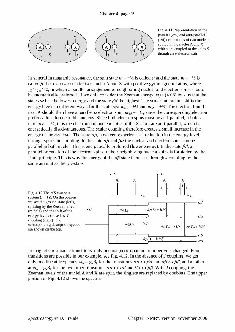
Fig. 4.11 Representation of the parallel (αα) and anti-parallel (αβ) orientations of two nuclear

.

cally preferred. If we only consider the Zeeman energy, equ. (4.08) tells us that the tate αα has the lowest energy and the state ββ the highest. The scalar interaction shifts the

ron

he

spins I in the nuclei A and X, which are coupled to the spins S though an s-electron pair

In general in magnetic resonance, the spin state m = +½ is called α and the state m = −½ is called β. Let us now consider two nuclei A and X with positive gyromagnetic ratios, where γX > γA > 0, in which a parallel arrangement of neighboring nuclear and electron spins should be energetisenergy levels in different ways: for the state αα, mIA = +½ and mIX = +½. The electron found near A should then have a parallel α electron spin, mSA = +½, since the corresponding electprefers a location near this nucleus. Since both electron spins must be anti-parallel, it holds that mSX = −½, thus the electron and nuclear spins of the X atom are anti-parallel, which is energetically disadvantageous. The scalar coupling therefore creates a small increase in tenergy of the αα level. The state αβ, however, experiences a reduction in the energy level through spin-spin coupling. In the state αβ and βα the nuclear and electron spins can be parallel in both nuclei. This is energetically preferred (lower energy). In the state ββ, a parallel orientation of the electron spins to their neighboring nuclear spins is forbidden by the Pauli principle. This is why the energy of the ββ state increases through J coupling by the same amount as the αα-state.

Fig. 4.12 The AX two spin ystem (I = ½). On the bottom s

we see the ground state (left), splitting by the Zeeman effect (middle) and the shift of the energy levels caused by J coupling (right). The corresponding absorption spectra are shown on the top. In magnetic resonance transitions, only one magnetic quantum number m is changed. Four transitions are possible in our example, see Fig. 4.12. In the absence of J coupling, we get only one line at frequency ωA = γABB d another t ωA = γXB0 for the two other transitions αα ↔ αβ and βα ↔ ββ. With J coupling, the

Zeeman levels of the nuclei A and X are split, the singlets are replaced by doublets. The upper portion of Fig. 4.12 shows the spectra.

0 for the transitions αα ↔ βα and αβ ↔ ββ, ana

A X

I S I S

α α

XA

I IS S

α β

P

E

hJ/4

hγAB0

hγXB0

hγAB0 + hJ/2

hγAB0 − hJ/2

hγXB0 − hJ/2 hγXB0 + hJ/2

P

J J A X A X

ν ν

αα

ββ

βα

αβ


Chapter 4, page 20

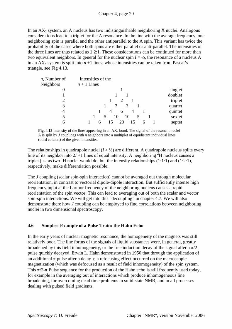
In an AX2 system, an A nucleus has two indistinguishable neighboriconsiderations lead to a triplet for the A resonance. In the line with t neighboring spin is parallel and the other antiparallel to the A spin. Tprobability of the cases where both spins are either parallel or anti-pthe three lines are thus related as 1:2:1. These considerations can betwo equivalent neighbors. In general for the nuclear spin I = ½, the resonance of a nucleus A in an AXn system is split into n +1 lines, whose intensities can be taken from Pascal’s triangle, see Fig 4.13.

uld do, but the intensity relationships (1:1:1) and (1:2:1), spectively, make differentiation possible.

he J coupling (scalar spin-spin interaction) cannot be averaged out through molecular orientation, in contrast to vectorial dipole-dipole interaction. But sufficiently intense high

armor frequency of the neighboring nucleus causes a rapid ctor. This can lead to averaging out of both the scalar and vector

will get into this "decoupling” in chapter 4.7. We will also oupling can be employed to find correlations between neighboring

l spectroscopy.

f a Pulse Train: the Hahn Echo

the early years of nuclear magnetic resonance, the homogeneity of the magnets was still latively poor. The line forms of the signals of liquid substances were, in general, greatly

f

.

ractions which produce inhomogeneous line roadening, for overcoming dead time problems in solid-state NMR, and in all processes

dealing with pulsed field gradients.

ng X nuclei. Analogous he average frequency, onehis variant has twice the

arallel. The intensities of continued for more than

n, Number of Intensities of the Neighbors n + 1 Lines

0 1 singlet 1 1 1 doublet 2 1 2 1 triplet 3 1 3 3 1 quartet 4 1 4 6 4 1 quintet 5 1 5 10 10 5 1 sextet 6 1 6 15 20 15 6 1 septet

Fig. 4.13 Intensity of the lines appearing in an AXn bond. The signal of the resonant nuclei A is split by J couplings with n neighbors into a multiplet of equidistant individual lines (third column) of the given intensities.

The relationships in quadrupole nuclei (I > ½) are different. A quadrupole nucleus splits every line of its neighbor into 2I +1 lines of equal intensity. A neighboring 2H nucleus causes a triplet just as two 1H nuclei wore Trefrequency input at the Lreorientation of the spin vespin-spin interactions. Wedemonstrate there how J cnuclei in two dimensiona

4.6 Simplest Example o

Inrebroadened by this field inhomogeneity, or the free induction decay of the signal after a π/2 pulse quickly decayed. Erwin L. Hahn demonstrated in 1950 that through the application oan additional π pulse after a delay τ, a refocusing effect occurred on the macroscopic magnetization (which was defocused as a result of field inhomogeneity) of the spin systemThis π/2-π Pulse sequence for the production of the Hahn echo is still frequently used today, for example in the averaging out of inteb


Chapter 4, page 21

We will clarify with the simplest model the action of the Hahn pulse group on a spin-spin system: a local magnetic field acts in addition to the external magnetic field, so that we have BBz = B0B + ΔBBz. From the laboratory coordinate system LAB we again move into the rotating coordinate system ROT, which rotates in the direction of the external magnetic field with the Larmor angular frequency ωL = γB0B , which is in resonance. In this case, the influence of the external magnetic field BB

the f llowing, we assume that τ « τ, τ is set by γBrfτπ/2 = π/2, and τ is the delay /2 pulse, the magnetization at time t = 0 flops

the π/2 pulse is so nged that it co nds with throscopic magn tion after th xROT-d

gnetization wou e conserved ductio angular quency ωL in th il lying in ence o tive or ative z-compon of the loc

0 = ωL/γ is no longer noticeable, in contrast to the local field which still is. In o π/2 π/2

between the two pulses. By applying a short πfrom dicular x-y-plane. If the phase of arra rrespo e yROT-direction of the rotating coordinate system, the

the z-direction into the perpen

ma etiz e π/2 pulse corresponds w ection. InROT

c a ith the ir the absence of an additional local field and other nuclear resonant interactions, the x ma ld b and produce an undamped free in n decay of

ffre e rf co the yLAB-direction. Under the influ the posig iel f t pne ent al f d ΔBB ucleu ins in rotating coordi system w th

z, the magnetization o his n s now she nate ith e angular frequency t

Δω = γΔBB (4.42)

.43)

ted to different local fields. This is the case when r

.

z and builds a phase angle (with the x-direction of the rotating coordinate system) α(t) = Δω t. (4

sample usually has areas which are subjecAthe additional local field is caused by an inhomogeneity in the external magnetic field, owhen an anisotropic chemical shift in a powder sample modifies the field acting on a nucleusBB in

e t = τ, a π pulse is applied. It has twice the length of a π/2 pulse, and its phase . The spin magnetization in all

nate system. The sign of te

)

efocused n

ID).

z and therefore also Δω and the phase angle α assume different positive or negative values these areas, and the macroscopic magnetization present after the π/2 pulse in the x-direction rapidly decays. The partial magnetization in the different areas are, after a certain time, evenly distributed in all directions in the x-y-plane, and no further signal is induced in the sample coil. At timcorresponds to the x-direction of the rotating coordinate systemareas of the sample turns 180° around the x-axis of the rotating coordithe phase angle α is thereby reversed by the π pulse at time t = τ. The spins continue to rotain the x-y-plane with Δω(r), but for the phase angle we now have α(r,t) = −α(r,τ)+Δω(r)·(t-τ). (4.44 If, after the π pulse, we again wait for time τ, t = 2τ. If we put this time into equ. (4.44) and compare to equ. (4.43), we see that α(r,2τ) = 0. With that, at time t = 2τ , the total macroscopic magnetization which dissipated under the influence of the local field is rand again dissipates when t > 2τ. In the rf coil, a signal is induced at time t = 2τ which is a"echo" of the free induction decay (F


Chapter 4, page 22

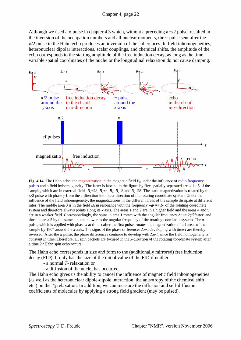
Although we used a π pulse in chapter 4.3 which, without a preceding a π/2 pulse, resultedthe inversion of the occupation numbers and all nuclear moments, the π pulse sent after the π/2 pulse in the Hahn echo produces an inversion of the coherences. In field inhomogeneitiesheteronuclear dipolar interactions, scalar couplings, and chemical shifts, the amplitude of the echo corresponds to the starting amplitude of the free induction decay, as long as the time-variable spatial coordinates of the nuclei or the longitudinal relaxation do not cause damping.

in

,

BB B BB0

M

x

y

z 0

M x

y

z 0

x

y

z

5 4

1 2

3

0

x

y

z

1 2

5 4

3

0

M x

y

z

π/2 pulse free induction decay π pulse echo around the in the rf coil around the in the rf coil y-axis in x-direction x-axis in x-direction

π/2 π

rf pulses

Fig. 4.14. The Hahn echo: the magnetization in the magnetic field BB0 under the influence of radio frequency pulses and a field imhomogeneity. The latter is labeled in the figure by five spatially separated areas 1 - 5 of the sample, which are in external fields B0B +2δ, B0+δ, B0, B0−δ and B0−2δ. The static magnetization is rotated by the π/2 pulse with phase y from the z-direction into the x-direction of the rotating coordinate system. Under the influence of the field inhomogeneity, the magnetizations in the different areas of the sample dissipate at different rates. The middle area 3 is in the field BB

weaker field. Correspondingly, the spins in area 1 rotate with the angular frequency Δω = 2γδ faster, and in area 5 by the same amount slower as the angular frequency of the rotating coordinate system. The π

of the

irrored) free induction

0 in resonance with the frequency −ωL=γ Β0 of the rotating coordinate system and therefore always points along its x axis. The areas 1 and 2 are in a higher field and the areas 4 and 5 are in athosepulse, which is applied with phase x at time τ after the first pulse, rotates the magnetization of all areas sample by 180° around the x-axis. The signs of the phase differences Δω t developing with time t are thereby reversed. After the π pulse, the phase differences continue to develop with Δω t, since the field homogeneity is constant in time. Therefore, all spin packets are focused in the x-direction of the rotating coordinate system after a time 2τ Hahn spin echo occurs.

he Hahn echo corresponds in size and form to the (additionally mTdecay (FID). It only has the size of the initial value of the FID if neither

- a normal T 2 relaxation or - a diffusion of the nuclei has occurred. The Hahn echo gives us the ability to cancel the influence of magnetic field inhomogeneities(as well as the heteronuclear dipole-dipole interaction, the anisotropy of the chemical shift, etc.) on the T2 relaxation. In addition, we can measure the diffusion and self-diffusion coefficients of molecules by applying a strong field gradient (may be pulsed).

t

magnetizatio

τ

free induction echo t

τ


Chapter 4, page 23

4.7 Two Dimensional NMR, Decoupling, Double Resonance

A one dimensional spectrum displays absorption as a function of resonant frequencies (usually as a δ-scale). It can be calculated from the time dependent free induction decay (FID)using one-dimensional Fourier transformation, as shown in chapter 4.2. Two dimensional pectra represent the absorption as a function of two quantities, for example the chemical shift

nd the J-coupling, or the chemical shift of two nuclei. The spectra with the two frequency

scales ω1 and ω2 are obtained from a two-dimensional Fourier transformation with respect to two independent variable times t1 and t2.

Decoupling is used to eliminate the influence of other nuclei on the nucleus to be examined. This involves inputting the resonant frequency of the other nuclei during signal measurement of the fr vel transitions in th ear spins of the other

Multip t of muexperiment. Double resonance is present in a limited sense, when by simultaneously irradiation of two nuclei, e.g. 1H and 13C, with the two correspondent Larmor frequencies, we get polarization transfer or coherence transfer between the two spin systems. In a simplified picture, the polarization corresponds to the magnetization of the undisturbed external magnetic field in the z-direction (different populations of the Zeeman levels), and the coherence corresponds to the transversal magnetization after a π/2 pulse. In quantum mechanics, the population probabilities are described by the diagonal elements and the transitions (coherences) by the elements in the first sub-diagonal of the spin density matrix.

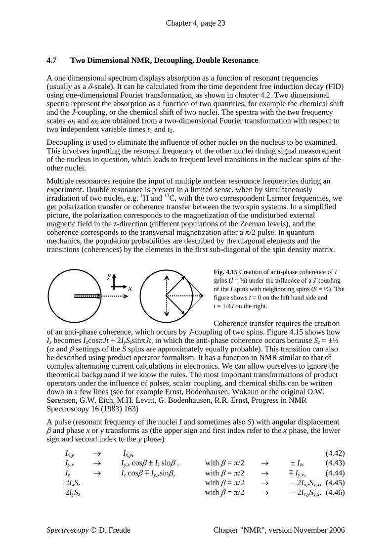
Fig. 4.15 Creation of anti-phase coherence of I spins (I = ½) under the influence of a J coupling

e he

evitt, G. Bodenhausen, R.R. Ernst, Progress in NMR

gular displacement and p and first index refer to the x phase, the lower

2) (4.43)

Iy,x, (4.44) 2IxSz with β = π/2 → − 2Ix,zSy,x, (4.45) 2IySz with β = π/2 → − 2Iz,ySy,x. (4.46)

sa

nucleus in question, which leads to equent le e nuclnuclei.

le resonances require the inpu ltiple nuclear resonance frequencies during an

of th I spins with neighboring spins (S = ½). Tfigure shows t = 0 on the left hand side and t = 1/4J on the right. Coherence transfer requires the creation

of an anti-phase coherence, which occurs by J-coupling of two spins. Figure 4.15 shows howIx becomes IxcosπJt + 2IySzsinπJt, in which the anti-phase coherence occurs because Sz = ±½ (α and β settings of the S spins are approximately equally probable). This transition can also be described using product operator formalism. It has a function in NMR similar to that of complex alternating current calculations in electronics. We can allow ourselves to ignore thetheoretical background if we know the rules. The most important transformations of productoperators under the influence of pulses, scalar coupling, and chemical shifts can be written down in a few lines (see for example Ernst, Bodenhausen, Wokaun or the original O.W.

ørensen, G.W. Eich, M.H. L

x y

SSpectroscopy 16 (1983) 163)

A pulse (resonant frequency of the nuclei I and sometimes also S) with anβ hase x or y transforms as (the upper signsign and second index to the y phase)

Ix,y → Ix,y, (4.4 Iy,x → Iy,x cosβ ± Iz sinβ , with β = π/2 → ± Iz, Iz → Iz cosβ m Iy,xsinβ, with β = π/2 → m


Chapter 4, page 24

Ix,y and Sx,y stand for single spin coherences and Ix,ySx,y for double spin coherences. The index z erences. Equations (4.45-

4.46) presume that pulses with corresponding phases act simultaneously on the I and S spin ces in

e

)

→ 2Ix,ySzcosπJt ± Iy,xsinπJt when Jt = ½ → ± Iy,x. (4.50)

)

using COR)

2 ω2

he 13C nuclei. Several spectra of this sort are taken for increasing values of t and then Fourier transformed into the second dimension with developed during the time t1, this is shown on the ω1correlation, cross signals only appear in 1H-13C orienother. This is an important aid in the ordering of the determination in complicated bonds. Fig 4.16 (Fig. 5 fromGriesinger, Angew. Chem. 100 (1988) 507) demons

describes the magnetizations. Mixed indices stand for anti-phase coh

systems. The pulses acting with the x phase transform as equ. (4.45) anti-phase coherendouble spin coherences; an anti-phase coherence of the I nuclei is transferred with the y phase to an anti-phase coherence of the S nuclei. In equ. (4.46), the effects in each pulse phase arexchanged.

Under the influence of the scalar coupling (πJtIzSz), we have the following transformations (the upper sign applies to the first index):

Iz → Iz (4.47 2IxSy → 2IxSy (4.48) Ix,y → Ix,ycosπJt ± 2Iy,xSzsinπJt when Jt = ½ → ± 2Iy,xSz, (4.49)

2Ix,ySz

Under the influence of the chemical shift (ΩtIz), we have the following transformations:

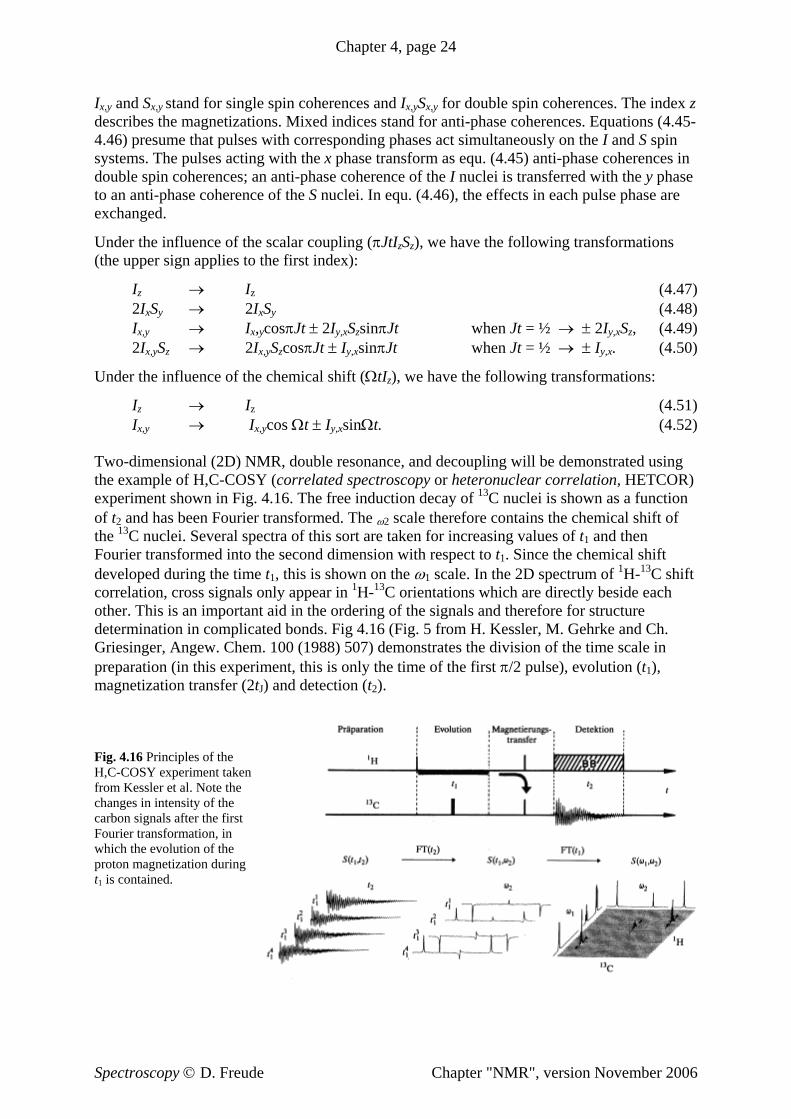
Iz → Iz (4.51) Ix,y → Ix,ycos Ωt ± Iy,xsinΩt. (4.52 Two-dimensional (2D) NMR, double resonance, and decoupling will be demonstratedthe example of H,C-COSY (correlated spectroscopy or heteronuclear correlation, HETexperiment shown in Fig. 4.16. The free induction decay of 13C nuclei is shown as a functionof t and has been Fourier transformed. The scale therefore contains the chemical shift of t 1

respect to t1. Since the chemical shift scale. In the 2D spectrum of H- C shift tations which are directly beside each signals and therefore for structure

H. Kessler, M. Gehrke and Ch.

1 13

trates the division of the time scale in preparation (in this experiment, this is only the time of the first π/2 pulse), evolution (t1), magnetization transfer (2tJ) and detection (t2).

Fig. 4.16 Principles of the H,C-COSY experiment taken from Kessler et al. Note the changes in intensity of the carbon signals after the first Fourier transformation, in which the evolution of the proton magnetization during t1 is contained.


Chapter 4, page 25

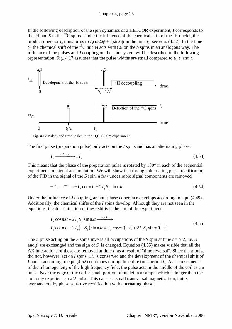
In the following description of the spin dynamics of a HETCOR experiment, I corresponds to the 1H and S to the 13C spins. Under the influence of the chemical shift of the 1H nuclei, the product operator Ix transforms to IxcosΩIt + IysinΩIt in the time t1, see equ. (4.52). In the timet

2, the chemical shift of the 13C nuclei acts with ΩS on the S spins in an analogous way. The

influence of the pulses and J coupling on the spin system will be described in the following representation. Fig. 4.17 assumes that the pulse widths are small compared to t1, tJ and t2.

π/2

π/2 π/2

1H

π t

0 t t1/2 1

lo t of th Deve pmen e 1H-spins 1H decoupling time

Detection of the 13C spins 2

time

3C 1

2tJ =1/J0

3)

54)

49). develop. Although they are not seen in the

s, the determination of these shifts is the aim of the experiment.

Fig. 4.17 Pulses and time scales in the H,C-COSY experiment. The first pulse (preparation pulse) only acts on the I spins and has an alternating phase:

( )I IzI

xyπ/2±⎯ →⎯⎯⎯ ± (4.5

This means that the phase of the preparation pulse is rotated by 180° in each of the sequential experiments of signal accumulation. We will show that through alternating phase rectification of the FID in the signal of the S spin, a few undesirable signal components are removed.

± ⎯ →⎯⎯ ± ±I I Jt I S JtxJ

x y zH-C cos sinπ π2 (4.

Under the influence of J coupling, an anti-phase coherence develops according to equ. (4.Additionally, the chemical shifts of the I spins equation

( )

( ) ( ) ( )I Jt I S Jt

I Jt I

x

x

cos

cos

π π

π

+ ⎯

+ 2

The π pulse acting on thand β are exchanged anAX interactions of thesedid not, however, act on

rding to equ.

S Jt I J t I S J ty z

S

y z x y z

xsin

sin cos sinπ π π

π →⎯⎯

− = − + −

2

2 (4.55)

e S spins inverts all occupations of the S spin at time t = t1/2, i.e. α d the sign of Sz is changed. Equation (4.55) makes visible that all the are removed at time t1 as a result of "time reversal". Since the π pulse I spins, ±Ix is conserved and the development of the chemical shift of (4.52) continues during the entire time period t1. As a consequence

the pulse acts in the middle of the coil as a π pulse. Near the edge of the coil, a small portion of nuclei in a sample which is longer than the coil only experience a π/2 pulse. This causes a small transversal magnetization, but is averaged out by phase sensitive rectification with alternating phase.

I nuclei accoof the inhomogeneity of the high frequency field,


Chapter 4, page 26

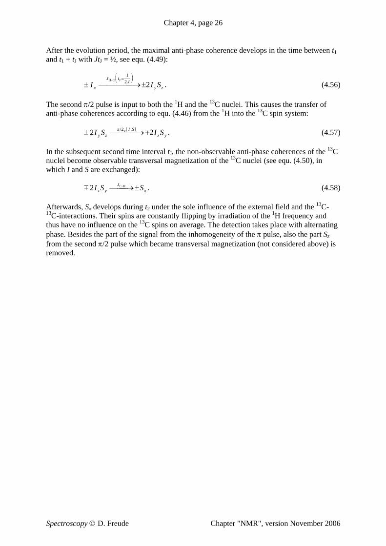
After the evolution period, the maximal anti-phase coherence develops in the time between t1 and t1 + tJ with JtJ = ½, see equ. (4.49):

± ⎯ →⎯⎯⎯⎯ ±=

⎛⎝⎜

⎞⎠⎟I I Sx

J tJ

y z

H-C J1

2 2 . (4.5

1 13

6)

he second π/2 pulse is input to both the H and the C nuclei. This causes the transfer of anti-phase coherences according to equ. (4.46) from the 1H into the 13C spin system:

. (4.57) In the subsequent second time interval tJ, the non-observable anti-phase coherences of the 13C nuclei become observable transversal magnetization of the 13C nuclei (see equ. (4.50), in which I and S are exchanged): . (4.58) Afterwards, Sx develops during t2 under the sole influence of the external field and the 13C-13C-interactions. Their spins are constantly flipping by irradiation of the 1H frequency and

detection takes place with alternating hase. Besides the part of the signal from the inhomogeneity of the π pulse, also the part Sz

e) is oved.

T

( )± ⎯ →⎯⎯⎯2 22I S I Sy zI S

z yxπ/ ,

m

m 2I S Sz yJ

xC-H⎯ →⎯⎯ ±

thus have no influence on the 13C spins on average. The pfrom the second π/2 pulse which became transversal magnetization (not considered abovrem


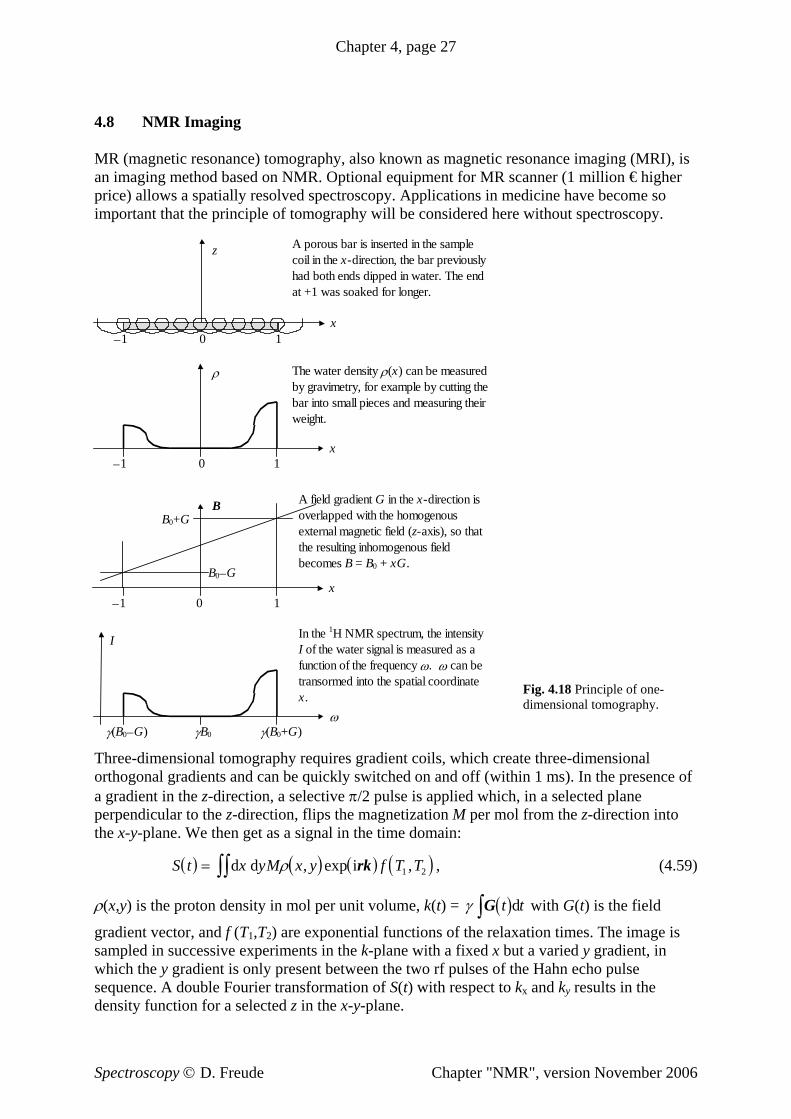
Chapter 4, page 27

4.8 NMR Imaging

MR (magnetic resonance) tomography, also known as magnetic resonance imaging (MRI), is n imaging method based on NMR. Orice) allows a spatially resolved spectroscopy. Applications in medicine have become so

Fig. 4.18 Principle of one-dimensional tomography.

Three-dimensional tomography requires gradient coils, which create three-dimensional orthogonal gradients and can be quickly switched on and off (within 1 ms). In the presence of a gradient in the z-direction, a selective π/2 pulse is applied which, in a selected plane perpendicular to the z-direction, flips the magnetization M per mol from the z-direction into the x-y-plane. We then get as a signal in the time domain:

a ptional equipment for MR scanner (1 million € higher pimportant that the principle of tomography will be considered here without spectroscopy.

( ) ( ) ( ) ( )S t x yM x y f T T= ∫∫ d d iρ , exp ,rk 1 2 , (4.59)

ρ(x,y) is the proton density in mol per unit volume, k(t) = ( )γ G t td∫ with G(t) is the field

gradient vector, and f (T1,T2) are exponential functions of the relaxation times. The image is sampled in successive experiments in the k-plane with a fixed x but a varied y gradient, in which the y gradient is only present between the two rf pulses of the Hahn echo pulse sequence. A double Fourier transformation of S(t) with respect to kx and ky results in the density function for a selected z in the x-y-plane.

−1 1 x

B

0

B0+G

B0−G

coil in the xhad both eat +1 was soaked for longer.

A porous bar is inserted in the sample -direction, the bar previously

nds dipped in water. The end

−1 1 x

0

z

The water density ρ(x) can be measured ρ by gravimetry, for example by cutting the

−1 1 x

0

γ(B0−G) γ(B0+G) ω

I

γB0

bar into small pieces and measuring their

overlapped with the homogenous external magnetic field (z-axis), so that the resulting inhomogenous field becomes B = B0 + xG.

In the 1H NMR spectrum, the intensity

weight.

A field gradient G in the x-direction is

I of the water signal is measured as a function of the frequency ω. ω can be transormed into the spatial coordinate x.


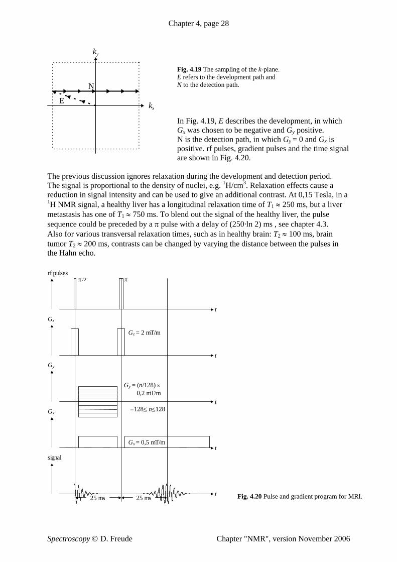
Chapter 4, page 28

Fig. 4.19 The sampling of the k-plane.

In Fig. 4.19, E describes the development, in which Gx was chosen to be negative and Gy positive. N is the detection path, in which Gy = 0 and Gx is positive. rf pulses, gradient pulses and the time signal are shown in Fig. 4.20.

The previous discussion ignores relaxation during the development and detection period. The signal is proportional to the density of nuclei, e.g. 1H/cm3. Relaxation effects cause a reduction in signal intensity and can be used to give an additional contrast. At 0,15 Tesla, in a 1H NMR signal, a healthy liver has a longitudinal relaxation time o T1 ≈ 250 ms, but a liver metastasis has one of T1 ≈ 750 ms. To blend out the signal of the healthy liver, the pulse sequence could be preceded by a π pulse with a delay of (250·ln 2) ms , see chapter 4.3. Also for various transversal relaxation times, such as in healthy brain: T2 ≈ 100 ms, brain tumor T2 ≈ 200 ms, contrasts can be changed by varying the distance between the pulses in the Hahn echo.

for MRI.

E refers to the development path and N to the detection path.

f

Fig. 4.20 Pulse and gradient program

E

N

kx

k

y

rf pulses

Gz

Gx

Gy

signal

25 ms 25 ms t

t

π /2 π

Gz = 2 mT/m

Gx = 0,5 mT/m

t

t

Gy = (n/128) × 0,2 mT/m −128≤ n≤128

t


Chapter 4, page 29

4.9 Literature

Abragam A.: The Principle of Nuclear MagnetisBigler P.: NMR Spectroscopy: Processing Strate eim 1997 Braun S., Kalinowski H.-O., Berger S.: 150 and ore Basic NMR Experiments, Wiley-VCH Weinheim 1998 Breitmaier E., Voelter W.: Carbon-13 NMR Spectroscopy, VHC Verlagsgesellschaft Weinheim 1987 Callaghan: Principles of NMR microscopy, Clarendon Press, 1991 Canet, D.: NMR-Konzepte und Methoden, SprinCroasmun, W.R. and R.M.K. Carlson: Two-Dim -3 Duer M. (ed.): Solid-state NMR, Blackwell ScieDybowski C., Lichter R.L.: NMR Spectroscopy Ernst R.R., Bodenhausen G. and Wokaun Pri

Press, 1986 Freemann R.: A Handbook of Nuclear Magnetic Resonance Spectroscopy, Longman, 1987

ding NMR Spectroscopy, Wiley, 2005 itamaru R.: Nuclear Magnetic Resonance, Principles and Theory, Elsevier, 1990

Kleinpeter E., Borsdorf R.: 13C-NMR in der organischen Chemie, Akademie Verlag, 1981 Mehring M.: Principles of High Resolution NMR in Solids, Springer-Verlag, 1983 Michel D.: Grundlagen und Methoden der kernmagnetischen Resonanz kademieverlag, 1982 Poole C.P. and Forach H.A.: Theory of Magnetic Resonance, Wiley 1987 Rahman A.: One and Two Dimensional NMR Spectroscopy, Elsevier, 89 Sanders J.K.M. and Hunter B.K.: Modern NMR Spectroscopy, Oxford niversity Press, 1987 Schraml J., Bellama J.M.: Two-Dimensional NMR Spectroscopy, John 988 Slichter C.P.: Principles of Magnetic Resonance, Springer-Verlag, 198Weber U., Thiele H., Hägele G.: NMR-Spectroscopy: Modern Spectral Analysis, Wiley-VCH Weinheim MRI in Medicine: M.T. Vlaardingerbroek, J.A. den Boer: Magnetic Resonance Imaging, ringer 2002 or M.T. Vlaardingerbroek,

J.A. den Boer: Magnetresonanzbildgebung, Springer 2004, ISBN 3 540 20028 2 R.H. Hashemi, W.G. Bradley: MRI the Basics; Williams & Wilkins 19 7 C.Westbrook, C.Kaut: MRI in Practice; Blackwell Science 1998 L.Dilcher, M.Venator, S.Dilcher: Kleines Handbuch der Kernspintomographie; Edwin Ferger Verlag 1997; ISBN

3-931219-02-X M. NessAiver: All you really need to know About MRI Physics; Simp Physics, Baltimore 1997, ISMN 0-

9660982-0-X

m, Oxford University Press, 1978 gies, Wiley-VCH Weinh

M

ger-Verlag, 1994, ISBN 3-540-58204-5 ensional NMR Spectroscopy, VCH, 1994, ISBN 1-560981-664nce, 2002, 0-632-05351-8 Techniques, Marcel Dekker, Inc., New York, 1987 nciples of NMR in One and Two Dimensions, Oxford University A.:

Friebolin H.: Basic One- and Two-Dimensional NMR-Spectroscopie, Wiley-VCH Weinheim, 1993 Fukushima E. Roeder S.B.W.: Experimental Pulse NMR, Addison-Wesley Publishing Company, Inc. 1981 Fyfe C.A.: Solid State NMR for Chemists, C.F.C. Press, 1983 Gerstein B.C., Dybowski C.R.: Transit Techniques in NMR of Solids, Academic Orlando, 1985 Günther H.: NMR Spektroskopie (1H NMR), Georg Thieme Verlag Stuttgart, 1983 Haeberlen U.: High Resolution NMR in Solids, Academic Press, 1976 Harris R.K.: Nuclear Magnetic Resonance Spectroscopy, Longman, 1986 Hennel, J.W.; Klinowski, J.: Fundamentals of NMR, Longman, Essex 1993, 288 S., ISBN 0 582 06703 0 Hesse M., Meier H., Zeeh B.: Spektroskopische Methoden in der organischen Chemie, Georg Thieme Verlag

Stuttgart, 1987 Keeler J.: UnderstanK

, A

19 U Wiley, 19

Sp

9

ly


4 Nuclear Magnetic Resonance - home.uni-leipzig.de · Chapter 4, page 4 Table 4.1 Gyromagnetic...

Documents

Transcript of 4 Nuclear Magnetic Resonance - home.uni-leipzig.de · Chapter 4, page 4 Table 4.1 Gyromagnetic...