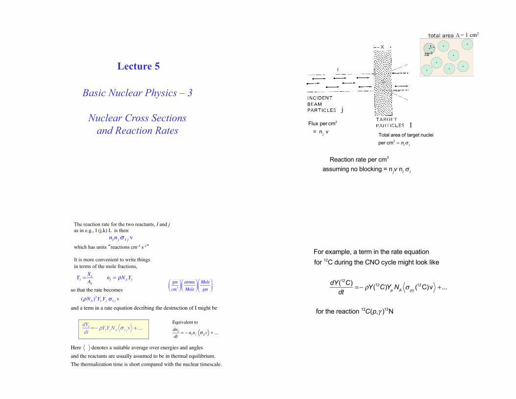
Lecture 5

Basic Nuclear Physics – 3

Nuclear Cross Sections and Reaction Rates

Flux per cm2

= n j v

Total area of target nuclei

per cm3 = nI σ I

Reaction rate per cm3 assuming no blocking = n jv nI σ I

j

I

= 1 cm2

The reaction rate for the two reactants, I and j as in e.g., I (j,k) L is then:

nInjσ I j vwhich has units �reactions cm-3 s-1� It is more convenient to write things in terms of the mole fractions,

YI =XI

AI

nI = ρNAYI

so that the rate becomes(ρNA )2YI Yj σ I j v

and a term in a rate equation decribing the destruction of I might be

dYIdt

=− ρYIYjNA σ I jv +....

Here denotes a suitable average over energies and anglesand the reactants are usually assumed to be in thermal equilibrium.The thermalization time is short compared with the nuclear timescale.

gm

cm3

⎛⎝⎜

⎞⎠⎟atoms

Mole

⎛⎝⎜

⎞⎠⎟

Mole

gm

⎛⎝⎜

⎞⎠⎟

Equivalent to

dnI

dt= − nInj σ Ijv + ...

For example, a term in the rate equationfor 12C during the CNO cycle might look like

dY(12C)dt

=− ρY(12C)Yp NA σ pγ (12C)v +...

for the reaction 12C(p,γ )13N

The cross section for reaction is defined in the usual way:

σ = number reactions/nucleus /secondnumber incident particles/cm2 / second

σ clearly has units of area (cm2 )For a Maxwell-Boltzmann distribution of reactant energies

The average of the cross section times velocity is

σ I jv = 8πµ

⎛⎝⎜

⎞⎠⎟

1/21

kT⎛⎝⎜

⎞⎠⎟

3/2

σ I j (E) E e−E /kT dE0

∞

∫

where µ is the "reduced mass"

µ=MIm j

MI+ m j

for the reaction I (j, k) L

v = 2Em

⎛⎝⎜

⎞⎠⎟

1/2

dv = 12

⎛⎝⎜

⎞⎠⎟

2mE

⎛⎝⎜

⎞⎠⎟

1/2

dE

σ v3 dv = σ 2Em

⎛⎝⎜

⎞⎠⎟

3/212

2mE

⎛⎝⎜

⎞⎠⎟

1/2

dE

= 2m2 σE dE

Center of mass system – that coordinate system in which the total initial momenta of the reactants is zero. The energy implied by the motion of the center of mass is not available to cause reactions.

1 2

1 2

Replace mass by the "reduced mass"

M M =

M Mµ

+

Read Clayton – Chapter 4.1

For T in 109 K = 1 GK, in barns (1 barn = 10-24 cm2), E6 in MeV, and k = 1/11.6045 MeV/GK, the thermally averaged rate factor in cm3 s-1 is

σjk

v = 6.197 x 10-14

A1/2T9

3/ 2σ

jk(E

6) E

6e−11.6045 E

6/T

9 dE6

0

∞

∫

A =A

IA

j

AI+ A

j

for the reaction I(j,k)L

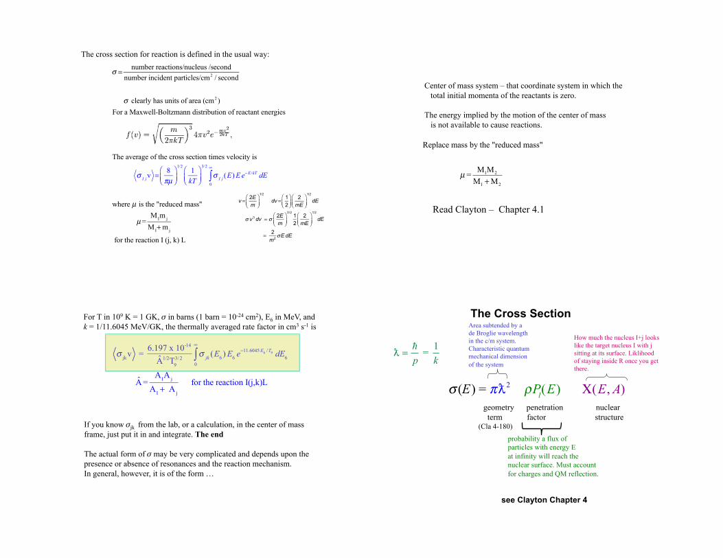
If you know jk from the lab, or a calculation, in the center of mass frame, just put it in and integrate. The end The actual form of may be very complicated and depends upon the presence or absence of resonances and the reaction mechanism. In general, however, it is of the form …

σ (E) = π2 ρP

l(E) Χ(E, A)

geometry penetration nuclear term factor structure

=

p =

1

k

How much the nucleus I+j looks like the target nucleus I with j sitting at its surface. Liklihood of staying inside R once you get there.

Area subtended by a de Broglie wavelength in the c/m system. Characteristic quantum mechanical dimension of the system

probability a flux of particles with energy E at infinity will reach the nuclear surface. Must account for charges and QM reflection.

The Cross Section

see Clayton Chapter 4

(Cla 4-180)

where is the de Broglie wavelenth in the c/m system

π2 = π2

µ2v2 =π2

2µE= 0.656barns

A E(MeV)

where 1 barn = 10-24 cm2 is large for a nuclear cross section.Note that generally E(MeV) < 1 and > Rnucleus but

is much smaller than the interparticle spacing.

µ=M1M 2

M1 +M 2

A=A1A2

A1 + A2

~ 1 for neutrons and protons

~ 4 for α-particles if AI is large

Clayton p. 319ff shows that Schroedinger'sequation for two interacting particles in a radial potential is given by (Cla 4-122) [see also our Lec 4]

Ψ(r, θ ,φ) = χ l (r)

rYl

m (θ ,φ)

where χ(r) satisfies

-2

2µd 2

dr 2 + l(l +1)2

2µr 2 +V (r) − E⎡

⎣⎢

⎤

⎦⎥ χ l (r)=0

V (r)=Z

IZ

je

2

rr >R

V (r)=V

nucr < R

for interacting particles with both charge and angular momentum. The angular momentum term represents the known eigenvalues of the operator L2 in a spherical potential

potential

(Clayton 4-103)

Consider just the barrier penetration part (R < r < infinity)

*The 1/r cancels the r2 when integrating Ψ*Ψ oversolid angles (e.g. Clayton 4-114). It is not part ofthe potential dependent barrier penetration calculation.

*

Classically, centrifugal force goes like

Fc = mv2

R= m2v2R2

mR3 = L2

mR3

One can associate a centrifugal potential with this,

Fc dR∫ = −L2

2mR2

Expressing things in the center of mass system and taking the usual QM eigenvaluens for the operator L2

one has

−l(l +1) 2

2µR2

To solve

-2

2µd 2

dr 2 + l(l +1)2

2µr 2 +V (r) − E⎡

⎣⎢

⎤

⎦⎥ χ l (r)=0

divide by E and substitute for V(r) for r >R

−2

2µEd 2

dr 2 + l(l +1)2

2µr 2E+

ZI Z je2

rE−1

⎡

⎣⎢⎢

⎤

⎦⎥⎥χ(r) =0

Change of radius variable. Substitute for r

ρ =2µE2 r dρ → 2µE

2 dr d 2ρ → 2µE2 d 2r

and for Coulomb interaction

η=ZI Z je

2

vv= 2E

µto obtain

−d 2

dρ2 + l(l +1)ρ2 + 2η

ρ−1

⎡

⎣⎢

⎤

⎦⎥ χ l (ρ)=0

chain rule

ρ and η are dimensionless numbers

where F and G, the regular and irregular Coulomb functions are the solutions of the differential equation and the constants come from applying the boundary conditions

d 2χdρ2 + (1− 2η

ρ− l(l +1)

ρ2 )χ = 0

has solutions (Abromowitz and Stegun 14.1.1)

χ = C1 Fl (η,ρ) + C2 Gl (η,ρ) C1 = 1 C2 = i

The barrier penetration function Pl is then given by

Pl =χ l (∞)

2

χ l (R)2 =

Fl2 (ρ = ∞)+Gl

2 (ρ = ∞)Fl2 (η,ρ)+Gl

2 (η,ρ)= 1Fl2 (η,ρ)+Gl

2 (η,ρ)

This is the solution for

R < r < ∞

For the one electron atom with

a potential Ze

2

r, one obtains the

same solution but the radial component

is Laguerre polynomials.

Cla 4-115

The “1” in the numerator corresponds to a purely outgoing wave at infinity from a decaying state.

http://people.math.sfu.ca/~cbm/aands/

multiply by -1

ρPl gives the probability of barrier penetration to the nuclear

radius R with angular momentum l. In general,

ρPl=

ρ

Fl

2 (η,ρ) +Gl

2 (η,ρ)where F

l is the regular Coulomb function

and Gl is the irregular Coulomb function

See Abramowitcz and Stegun, Handbook of Mathematical Functions, p. 537

These are functions of the dimensionless variables

η=Z

IZ

je2

v=0.1575Z

IZ

jA / E

ρ=2µE

2

R=0.2187 AE Rfm

e.g., Illiadis 2.162

contains all the charge dependence contains all the radius dependence

Physical meaning of η=Z

IZ

je

2

v

The classical turning radius, r0, is given by

1

2µv

2 = Z

IZ

je

2

r0

The de Broglie wavelength on the other hand is

=

p=

µv

Hence η=r

0

2

The probability of finding the particle inside of its classical turning

radius decreases exponentially with this ratio.

., both and are dimensionless.nb η ρ

ro=2Z

IZje2

µv2=η

2

µv=2η

On the other hand,

ρ=2µE

2

R =R

is just the size of the nucleus measured in de Broglie

wavelengths.

This enters in, even when the angular momentum and

charges are zero, because an abrupt change in potential

at the nuclear surface leads to reflection of the wave

function.

=

p=

µv=

2 µ( )1

2µv2

⎛⎝⎜

⎞⎠⎟

For low interaction energy, (2η>>ρ, i.e., E << ZI Z je

2

R)

and Zj ≠0, ρPl has the interesting limit

ρPl ≈ 2ηρ exp −2πη+4 2ηρ − 2l(l +1)

2ηρ

⎡

⎣⎢⎢

⎤

⎦⎥⎥

where

2ηρ = 0.2625 ZI Z j ARfm( )1/2

which is independent of energy but depends on nuclear size.

Note: rapid decrease with smaller energy and increasing charge(η ↑ ) rapid decrease with increasing angular momentum

The leading order term for l = 0 proportional to

ρPl ∝ exp −2πη( )

Abramowitz and Stegun, 14.6.7

η=ZIZ j e

2

v=0.1575ZIZ j A / E

ρ = 2µE2

R=0.2187 AE Rfm

independent of E and l

There exist other interesting limits for ρPl,

for example when η is small - as for neutrons where it is 0

ρ∝E1/2 ρ P0=ρ

ρ P1=

ρ3

1+ρ2

ρP2=

ρ5

9 + 3ρ2+ρ4

This implies that for l = 0 neutrons the cross section will go as 1/v.

i.e., π2 ρ P

0∝

E1/ 2

E∝ E

−1/ 2

ρ <<1 for cases of interest for neutron capture

For low energy neutron induced reactions, the

cross section times velocity, i.e., the reaction rate

term, is approximately a constant

η=Z

IZ

je2

v= 0

ρ=2µE

2

R=0.2187 AE Rfm

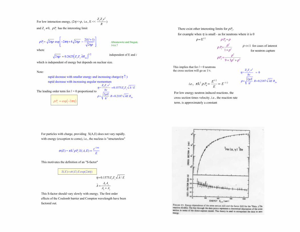
For particles with charge, providing X(A,E) does not vary rapidly.with energy (exception to come), i.e., the nucleus is "structureless"

σ (E) = π2ρPl X ( A, E) ∝ e−2πη

E

This motivates the definition of an "S-factor"

S(E)=σ (E) E exp(2πη)

η=0.1575ZI Z j A / E

A =AI Aj

AI + Aj

This S-factor should vary slowly with energy. The first order effects of the Coulomb barrier and Compton wavelength have beenfactored out.

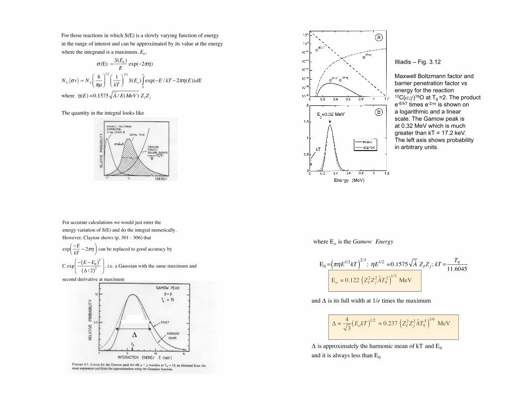
For those reactions in which S(E) is a slowly varying function of energy in the range of interest and can be approximated by its value at the energy where the integrand is a maximum, E0,

σ (E) S(E0 )E

exp(−2πη)

NA σ v ≈ NA8πµ

⎛⎝⎜

⎞⎠⎟

1/21kT

⎛⎝⎜

⎞⎠⎟

3/2

S(Eo ) exp(−E / kT −2πη(E))dE0

∞

∫where η(E) =0.1575 A / E(MeV ) ZIZ j

The quantity in the integral looks like

Illiadis – Fig. 3.12 Maxwell Boltzmann factor and barrier penetration factor vs energy for the reaction 12C(,)16O at T8 =2. The product e-E/kT times e-2 is shown on a logarithmic and a linear scale. The Gamow peak is at 0.32 MeV which is much greater than kT = 17.2 keV. The left axis shows probability in arbitrary units.

For accurate calculations we would just enter the energy variation of S(E) and do the integral numerically. However, Clayton shows (p. 301 - 306) that

exp −EkT

− 2πη⎛⎝⎜

⎞⎠⎟ can be replaced to good accuracy by

C exp− E − E0( )2

Δ / 2( )2⎛

⎝⎜

⎞

⎠⎟ , i.e. a Gaussian with the same maximum and

second derivative at maximum

'

where Eo is the Gamow Energy

E0 = πηE1/2kT( )2/3; ηE1/2 =0.1575 A ZIZ j; kT = T9

11.6045

Eo = 0.122 ZI2Z j

2AT92( )1/3

MeV

and Δ is its full width at 1/e times the maximum

Δ = 43EokT( )1/2 = 0.237 ZI

2Z j2AT9

5( )1/6 MeV

Δ is approximately the harmonic mean of kT and E0

and it is always less than E0

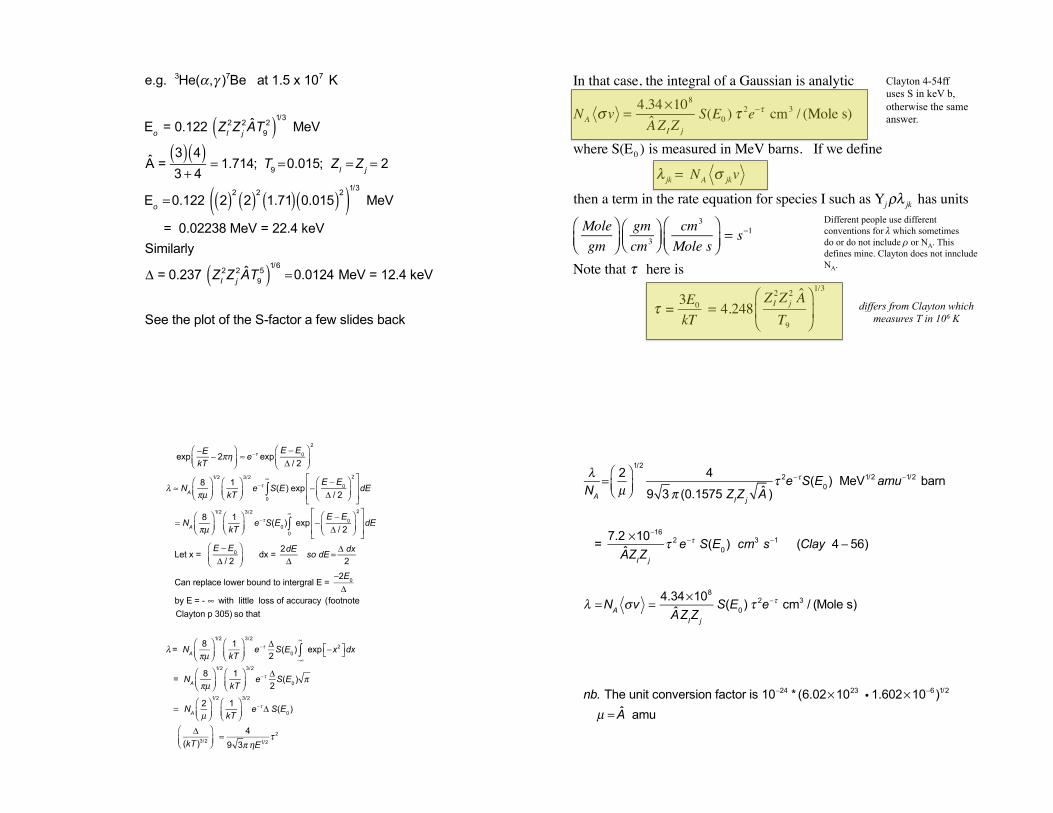
e.g. 3He(α,γ )7Be at 1.5 x 107 K

Eo = 0.122 ZI2Zj

2AT92( )1/3

MeV

A =3( ) 4( )3 + 4

= 1.714; T9 =0.015; ZI =Zj = 2

Eo =0.122 2( )22( )2

1.71( ) 0.015( )2( )1/3

MeV

= 0.02238 MeV = 22.4 keVSimilarly

Δ = 0.237 ZI2Zj

2AT95( )1/6

=0.0124 MeV = 12.4 keV

See the plot of the S-factor a few slides back

In that case, the integral of a Gaussian is analytic

NA σ v = 4.34×108

A ZIZ j

S(E0 ) τ 2e−τ cm3 / (Mole s)

where S(E0 ) is measured in MeV barns. If we define

λ jk = NA σ jkv

then a term in the rate equation for species I such as Yjρλ jk has units

Molegm

⎛⎝⎜

⎞⎠⎟

gmcm3

⎛⎝⎜

⎞⎠⎟

cm3

Mole s⎛⎝⎜

⎞⎠⎟= s−1

Note that τ here is

τ = 3E0

kT= 4.248

ZI2Z j

2 AT9

⎛

⎝⎜

⎞

⎠⎟

1/3

Different people use different conventions for which sometimes do or do not include or NA. This defines mine. Clayton does not innclude NA.'

Clayton 4-54ff uses S in keV b, otherwise the same answer.

differs from Clayton which measures T in 106 K

exp−EkT

− 2πη⎛⎝⎜

⎞⎠⎟≈ e−τ exp

E −E0

Δ / 2⎛⎝⎜

⎞⎠⎟

2

λ ≈ NA

8πµ

⎛⎝⎜

⎞⎠⎟

1/21

kT⎛⎝⎜

⎞⎠⎟

3/2

e−τ S(E) exp −E −E0

Δ / 2⎛⎝⎜

⎞⎠⎟

2⎡

⎣⎢⎢

⎤

⎦⎥⎥0

∞

∫ dE

= NA

8πµ

⎛⎝⎜

⎞⎠⎟

1/21

kT⎛⎝⎜

⎞⎠⎟

3/2

e−τS(E0) exp −E −E0

Δ / 2⎛⎝⎜

⎞⎠⎟

2⎡

⎣⎢⎢

⎤

⎦⎥⎥0

∞

∫ dE

Let x = E −E0

Δ / 2⎛⎝⎜

⎞⎠⎟

dx = 2dEΔ

so dE = Δ dx2

Can replace lower bound to intergral E = −2E0

Δ

by E = - ∞ with little loss of accuracy (footnote Clayton p 305) so that

λ= NA

8πµ

⎛⎝⎜

⎞⎠⎟

1/21

kT⎛⎝⎜

⎞⎠⎟

3/2

e−τ Δ2

S(E0) exp −x2⎡⎣ ⎤⎦−∞

∞

∫ dx

= NA

8πµ

⎛⎝⎜

⎞⎠⎟

1/21

kT⎛⎝⎜

⎞⎠⎟

3/2

e−τ Δ2

S(E0) π

= NA

2µ

⎛⎝⎜

⎞⎠⎟

1/21

kT⎛⎝⎜

⎞⎠⎟

3/2

e−τ Δ S(E0)

Δ(kT )3/2

⎛⎝⎜

⎞⎠⎟

= 4

9 3π ηE1/2τ 2

λNA

= 2µ

⎛⎝⎜

⎞⎠⎟

1/24

9 3π (0.1575 ZIZ j A )τ 2e−τS(E0) MeV1/2 amu−1/2 barn

= 7.2 ×10−16

AZIZ j

τ 2 e−τ S(E0) cm3 s−1 (Clay 4 − 56)

λ =NA σv = 4.34×108

AZIZ j

S(E0) τ 2e−τ cm3 / (Mole s)

nb. The unit conversion factor is 10−24 * (6.02×1023 i 1.602×10−6)1/2

µ = A amu

Adelberger et al, RMP, (1998( f = τ

2e−τ

τ =A

T1/3

dτ

dT= −

A

3T 4/3=−

τ

3T

df

dT=2τe−τ

dτ

dT− τ

2e−τ dτ

dT

T

f

df

dT

⎛⎝⎜

⎞⎠⎟=

T

τ2e−τ

(2τ e−τ )(−τ

3T) −

T

τ2e−τ

(τ 2e−τ )(−

τ

3T)

=d ln f

d lnT

⎛⎝⎜

⎞⎠⎟=τ − 2

3

∴ f ∝ T n n=τ − 2

3

For example, 12C + 12C at 8 x 108 K

τ =4.24862 62 12⋅12

12+12

0.8

⎛

⎝⎜⎜

⎞

⎠⎟⎟

1/3

= 90.66

n = 90.66− 23

= 29.5

p + p at 1.5 x 107 K

τ = 4.248

1⋅1⋅1⋅11+1

0.015

⎛

⎝

⎜⎜⎜

⎞

⎠

⎟⎟⎟

1/3

= 13.67

n = 13.67 - 2

3= 3.89

Thus �non-resonant� reaction rates will have a temperature dependence of the form

λ

Constant

T2/3exp(−

constant

T1/3)

This is all predicated upon S(Eo ) being constant, or at least slowly varying. This will be the case provided: i) E << ECoul ; l = 0 ii) All narrow resonances, if any, lie well outside the Gamow �window�

E

o± Δ / 2

That is there are no resonances or there are very many overlapping resonances iii) No competing reactions (e.g., (p,n), (p,) vs (p,)) open up in the Gamow window

τ2e−τ

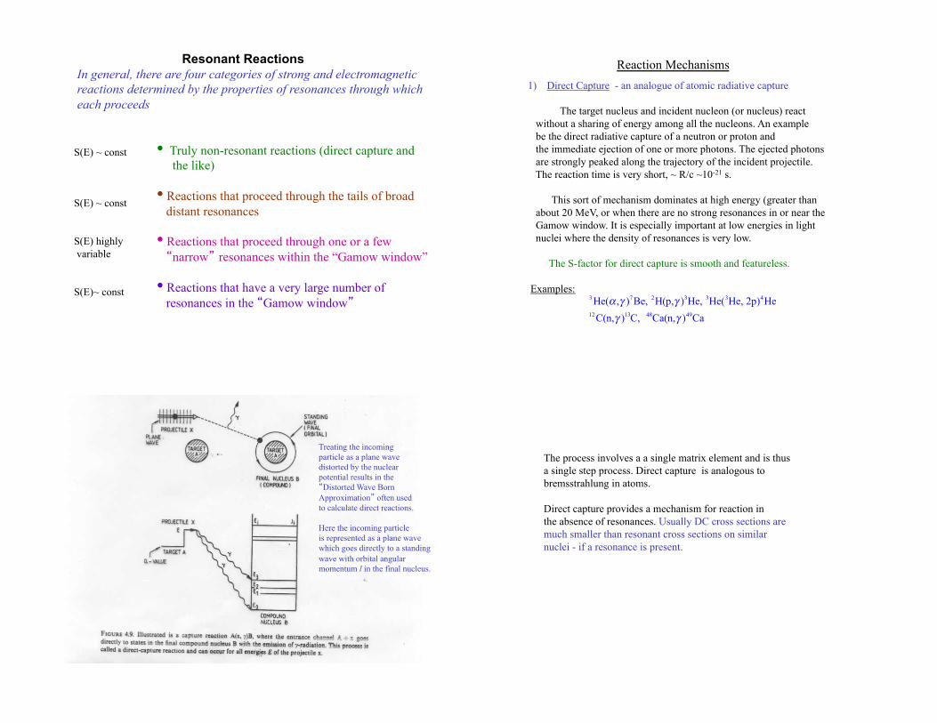
In general, there are four categories of strong and electromagnetic reactions determined by the properties of resonances through which each proceeds

•  Truly non-resonant reactions (direct capture and the like) •  Reactions that proceed through the tails of broad distant resonances •  Reactions that proceed through one or a few �narrow��resonances within the “Gamow window” •  Reactions that have a very large number of resonances in the �Gamow window�

S(E) ~ const S(E) ~ const S(E) highly variable S(E)~ const

Resonant Reactions Reaction Mechanisms 1)  Direct Capture - an analogue of atomic radiative capture

The target nucleus and incident nucleon (or nucleus) react without a sharing of energy among all the nucleons. An example be the direct radiative capture of a neutron or proton and the immediate ejection of one or more photons. The ejected photons are strongly peaked along the trajectory of the incident projectile. The reaction time is very short, ~ R/c ~10-21 s. This sort of mechanism dominates at high energy (greater than about 20 MeV, or when there are no strong resonances in or near the Gamow window. It is especially important at low energies in light nuclei where the density of resonances is very low. The S-factor for direct capture is smooth and featureless. Examples:

3 He(α ,γ )7Be, 2H(p,γ )3He, 3He(3He, 2p)4He

12C(n,γ )13C, 48Ca(n,γ )49Ca

Treating the incoming particle as a plane wave distorted by the nuclear potential results in the �Distorted Wave Born Approximation� often used to calculate direct reactions. Here the incoming particle is represented as a plane wave which goes directly to a standing wave with orbital angular momentum l in the final nucleus.

The process involves a a single matrix element and is thus a single step process. Direct capture is analogous to bremsstrahlung in atoms. Direct capture provides a mechanism for reaction in the absence of resonances. Usually DC cross sections are much smaller than resonant cross sections on similar nuclei - if a resonance is present.

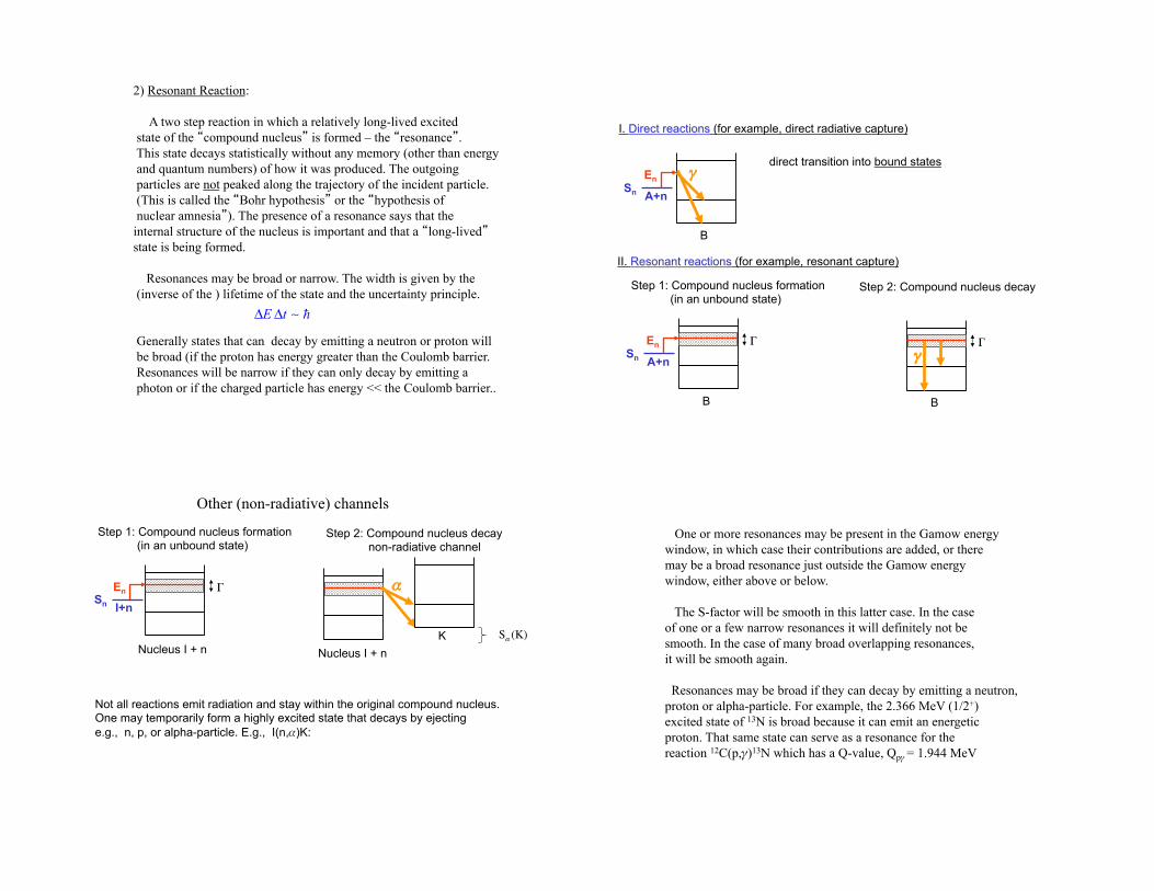
2) Resonant Reaction: A two step reaction in which a relatively long-lived excited state of the �compound nucleus� is formed – the �resonance�. This state decays statistically without any memory (other than energy and quantum numbers) of how it was produced. The outgoing particles are not peaked along the trajectory of the incident particle. (This is called the �Bohr hypothesis� or the �hypothesis of nuclear amnesia�). The presence of a resonance says that the internal structure of the nucleus is important and that a �long-lived� state is being formed. Resonances may be broad or narrow. The width is given by the (inverse of the ) lifetime of the state and the uncertainty principle. Generally states that can decay by emitting a neutron or proton will be broad (if the proton has energy greater than the Coulomb barrier. Resonances will be narrow if they can only decay by emitting a photon or if the charged particle has energy << the Coulomb barrier..

ΔEΔt

I. Direct reactions (for example, direct radiative capture)

A+n

B

En Sn

'direct transition into bound states

II. Resonant reactions (for example, resonant capture)

A+n

B

En Sn

Step 1: Compound nucleus formation (in an unbound state)

'

B

Step 2: Compound nucleus decay

''

Not all reactions emit radiation and stay within the original compound nucleus. One may temporarily form a highly excited state that decays by ejecting e.g., n, p, or alpha-particle. E.g., I(n,)K:

Nucleus I + n

En

Step 1: Compound nucleus formation (in an unbound state)

'

Nucleus I + n

Step 2: Compound nucleus decay non-radiative channel

'

K

I+n Sn

Sα(K)

Other (non-radiative) channels

One or more resonances may be present in the Gamow energy window, in which case their contributions are added, or there may be a broad resonance just outside the Gamow energy window, either above or below. The S-factor will be smooth in this latter case. In the case of one or a few narrow resonances it will definitely not be smooth. In the case of many broad overlapping resonances, it will be smooth again. Resonances may be broad if they can decay by emitting a neutron, proton or alpha-particle. For example, the 2.366 MeV (1/2+) excited state of 13N is broad because it can emit an energetic proton. That same state can serve as a resonance for the reaction 12C(p,)13N which has a Q-value, Qp = 1.944 MeV

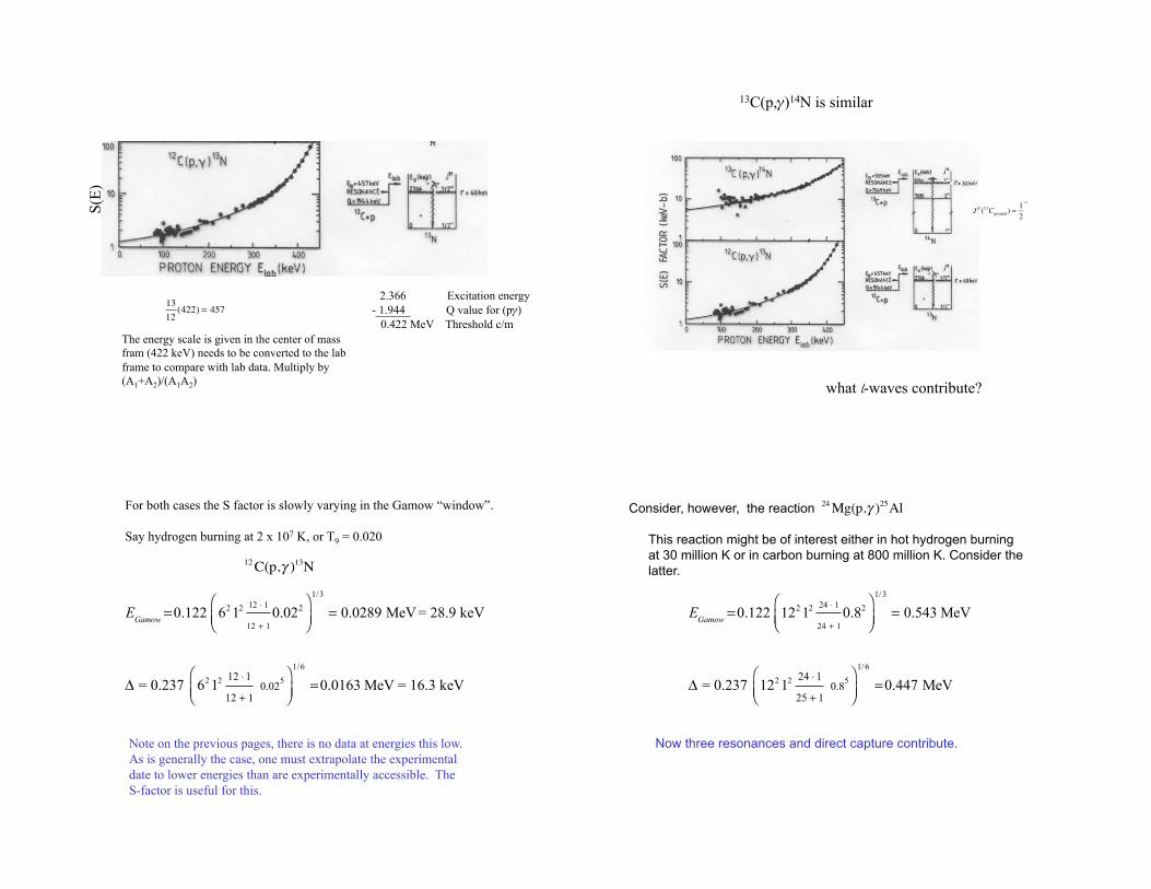
2.366 Excitation energy - 1.944 Q value for (p) 0.422 MeV Threshold c/m

13

12(422) = 457

S(E)

The energy scale is given in the center of mass fram (422 keV) needs to be converted to the lab frame to compare with lab data. Multiply by (A1+A2)/(A1A2)

13C(p,)14N is similar

J π (13Cground ) =12

−

what l-waves contribute?

EGamow

=0.122 621

212 ⋅ 1

12 + 1

0.022

⎛⎝⎜

⎞⎠⎟

1/3

= 0.0289 MeV = 28.9 keV

Δ = 0.237 621

212 ⋅1

12 + 1

0.025

⎛⎝⎜

⎞⎠⎟

1/6

=0.0163 MeV = 16.3 keV

For both cases the S factor is slowly varying in the Gamow “window”. Say hydrogen burning at 2 x 107 K, or T9 = 0.020

Note on the previous pages, there is no data at energies this low. As is generally the case, one must extrapolate the experimental date to lower energies than are experimentally accessible. The S-factor is useful for this.

12C(p,γ )13N

EGamow

=0.122 1221

224 ⋅ 1

24 + 1

0.82

⎛⎝⎜

⎞⎠⎟

1/3

= 0.543 MeV

Δ = 0.237 1221

224 ⋅1

25 + 1

0.85

⎛⎝⎜

⎞⎠⎟

1/6

=0.447 MeV

This reaction might be of interest either in hot hydrogen burning at 30 million K or in carbon burning at 800 million K. Consider the latter.

Now three resonances and direct capture contribute.

24Mg(p,γ )25AlConsider, however, the reaction

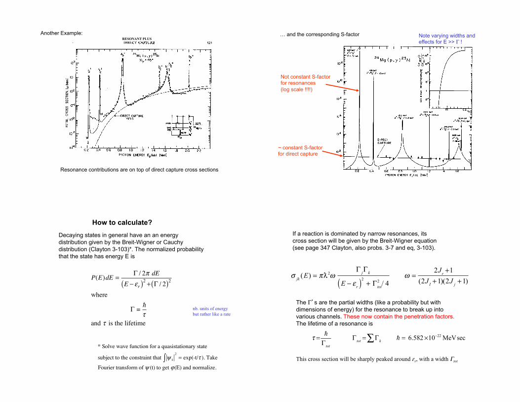
Another Example:

Resonance contributions are on top of direct capture cross sections

RESONANT PLUS … and the corresponding S-factor

~ constant S-factor for direct capture

Not constant S-factor for resonances (log scale !!!!)

Note varying widths and effects for E >> !

Decaying states in general have an an energy distribution given by the Breit-Wigner or Cauchy distribution (Clayton 3-103)*. The normalized probability that the state has energy E is

P(E)dE =Γ / 2π dE

E − εr( )

2+ Γ / 2( )

2

where

Γ =

τ

and τ is the lifetime

* Solve wave function for a quasistationary state

subject to the constraint that ψ k∫2= exp(-t/τ ). Take

Fourier transform of ψ (t) to get ϕ(E) and normalize.

nb. units of energy but rather like a rate

How to calculate? If a reaction is dominated by narrow resonances, its cross section will be given by the Breit-Wigner equation (see page 347 Clayton, also probs. 3-7 and eq, 3-103).

σjk

(E) = π2ω

ΓjΓ

k

E − εr( )

2

+ Γtot

2 / 4ω =

2Jr+1

(2JI+1)(2J

j+1)

The �s are the partial widths (like a probability but with dimensions of energy) for the resonance to break up into various channels. These now contain the penetration factors. The lifetime of a resonance is

τ =

Γtot

Γtot= Γ

k∑ = 6.582×10−22MeVsec

This cross section will be sharply peaked around r, with a width tot

Γtot

= Γi∑

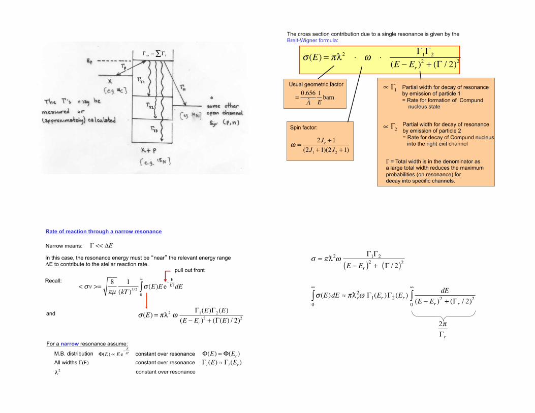
The cross section contribution due to a single resonance is given by the Breit-Wigner formula:

σ (E) = π2

⋅ ω ⋅Γ1Γ2

(E − Er)2+ (Γ / 2)

2

ω =2J

r+1

(2J1+1)(2J

2+1)

Usual geometric factor

=0.656

A

1

Ebarn

Spin factor:

1Γ∝ Partial width for decay of resonance

by emission of particle 1 = Rate for formation of Compund nucleus state

2Γ∝ Partial width for decay of resonance

by emission of particle 2 = Rate for decay of Compund nucleus into the right exit channel

= Total width is in the denominator as a large total width reduces the maximum probabilities (on resonance) for decay into specific channels.

Rate of reaction through a narrow resonance

Narrow means: Γ << ΔE

In this case, the resonance energy must be �near� the relevant energy range E to contribute to the stellar reaction rate.

Recall: < σv >=

8

πµ

1

(kT )3/2

σ (E)E e−E

kT

0

∞

∫ dE

and

σ (E) = π2ω

Γ1(E)Γ

2(E)

(E − Er)2+ (Γ(E) / 2)

2

For a narrow resonance assume:

M.B. distribution Φ(E)∝ E e−E

kT constant over resonance All widths (�) !

Φ(E) ≈ Φ(Er)

constant over resonance Γi(E) ≈ Γ

i(E

r)

2 constant over resonance

pull out front

σ = π2ωΓ1Γ2

E − Er( )2+   Γ / 2( )

2

σ (E)dE ≈ πr

2ω Γ1(Er )0

∞

∫ Γ2 (Er )dE

(E − Er)2+ (Γ

r/ 2)

2

0

∞

∫

2π

Γr

Then one can carry out the integration analytically (Clayton 4-193) and finds:

NA< σv >= 1.54 ⋅10

11(AT9 )

−3/2ωγ [MeV]e

−11.605 Er

[MeV]

T9

cm3

s mole

ωγ =2J

r+1

(2Jj+1)(2J

I+1)

Γ1Γ2

Γ

For the contribution of a single narrow resonance to the stellar reaction rate:

The rate is entirely determined by the �resonance strength��!ωγ

Which in turn depends mainly on the total and partial widths of the resonance at resonance energies.

Often Γ = Γ1+ Γ

2Then for

1

21

221Γ≈

Γ

ΓΓ⎯→⎯Γ≈Γ⎯→⎯Γ<<Γ

Γ2<< Γ

1⎯→⎯ Γ ≈ Γ

1⎯→⎯

Γ1Γ2

Γ≈ Γ

2

And reaction rate is determined by the smaller one of the widths !

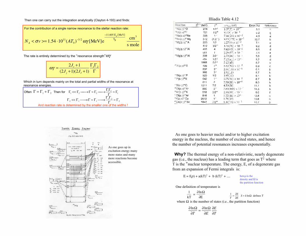
Illiadis Table 4.12

As one goes up in excitation energy many more states and many more reactions become accessible.

here is the density and is the partition function

As one goes to heavier nuclei and/or to higher excitation energy in the nucleus, the number of excited states, and hence the number of potential resonances increases exponentially. Why? The thermal energy of a non-relativistic, nearly degenerate gas (i.e., the nucleus) has a leading term that goes as T2 where T is the �nuclear temperature. The energy, E, of a degenerate gas from an expansion of Fermi integrals is:

E = f(ρ) + a(kT)2+ b (kT)4 + ....

One definition of temperature is

1

kT =

∂ lnΩ

∂E

where Ω is the number of states (i.e., the partition function)

∂ lnΩ

∂T=∂ lnΩ

∂E

∂E

∂T

1

T=∂S

∂ES = k lnΩ defines T

The number of excited states (resonances) per unit excitation energy increases exponentialy with excitation energy.

d lnΩ ~1

kT

∂E∂T

⎛⎝⎜

⎞⎠⎟

dT ~ 1

kT2ak2T( )  dT

ln Ω ~ 2ak dT∫ = 2akT + const

Ω ~ C exp 2akT( )

and if we identify the excitation energy, Ex ≈ a(kT)2,

i.e., the first order thermal correction to the internal energy, then

kT( )2

~ Ex

a

Ω = C exp 2 aEx( )Empirically a ≈ A/9. There are corrections to a for shell

and pairing effects. In one model (back-shifted Fermi gas)

C = 0.482

A5/6Ex

3/2

Generate an energy averaged cross section

σ =σ (E)dE

E

E+ΔE

∫ΔE

∝ 1ΔE 1

N

∑ω Γ j Γ k dE

(E − ε r )2 + Γ r2 / 4E

E+ΔE

∫

≈ω Γ jΓ k

ΔEN dE

(E − ε r )2 +Γ r2 / 40

∞

∫

D

Take N (>>1) equally spaced identical resonances in an energy interval E. For example, assume they all have the same partial widths.

dE

(E − εr)2 + Γ

r

2 / 40

∞

∫ =2π

Γr

N

ΔE=1

D

σ = 2π22ωΓjΓk

ΓrD

=π2ωTjTk

Ttot

where Tj=2π

Γj

D

D << E

E

What is the cross section when the density of resonances is large?

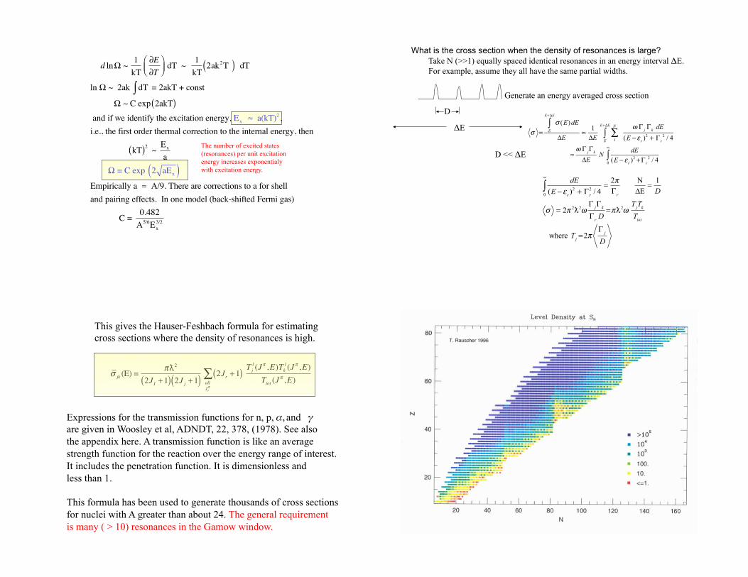
This gives the Hauser-Feshbach formula for estimating cross sections where the density of resonances is high.

σ jk (E) =π

2

2JI +1( ) 2J j +1( )2Jr +1( )

all

Jrπ

∑Tj

l(J

π,E)Tk

l(J

π,E)

Ttot (Jπ,E)

Expressions for the transmission functions for n, p, , and 'are given in Woosley et al, ADNDT, 22, 378, (1978). See also the appendix here. A transmission function is like an average strength function for the reaction over the energy range of interest. It includes the penetration function. It is dimensionless and less than 1. This formula has been used to generate thousands of cross sections for nuclei with A greater than about 24. The general requirement is many ( > 10) resonances in the Gamow window.

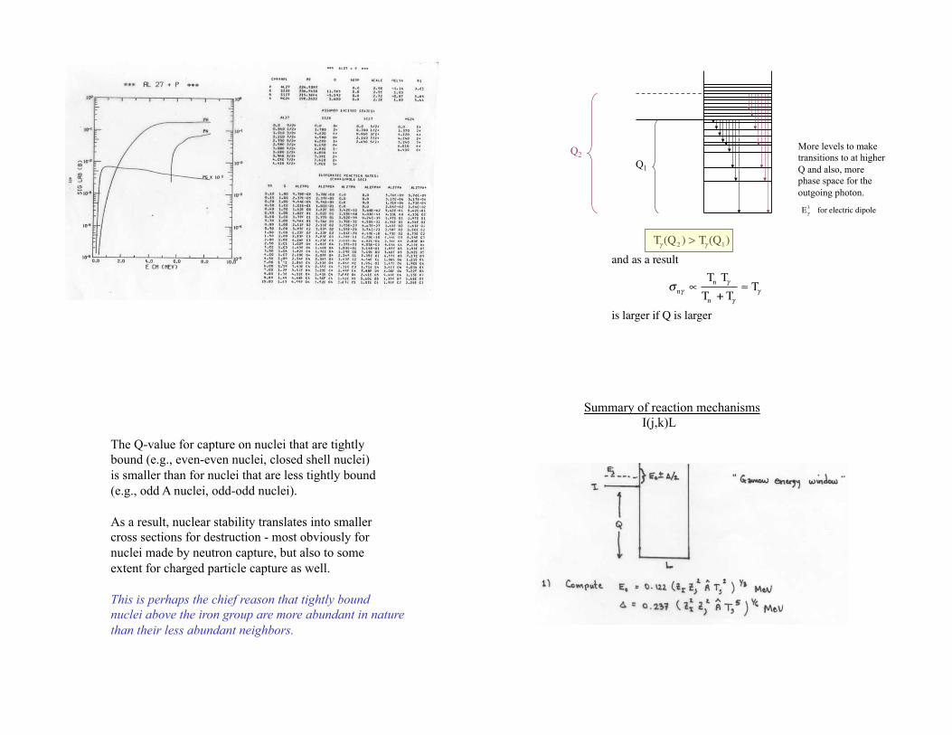
Q2 Q1

Tγ (Q2 ) > Tγ (Q1)

and as a result

σ nγ ∝Tn Tγ

Tn + Tγ

≈ Tγ

is larger if Q is larger

More levels to make transitions to at higher Q and also, more phase space for the outgoing photon.

Eγ

3 for electric dipole

The Q-value for capture on nuclei that are tightly bound (e.g., even-even nuclei, closed shell nuclei) is smaller than for nuclei that are less tightly bound (e.g., odd A nuclei, odd-odd nuclei). As a result, nuclear stability translates into smaller cross sections for destruction - most obviously for nuclei made by neutron capture, but also to some extent for charged particle capture as well. This is perhaps the chief reason that tightly bound nuclei above the iron group are more abundant in nature than their less abundant neighbors.

Summary of reaction mechanisms I(j,k)L

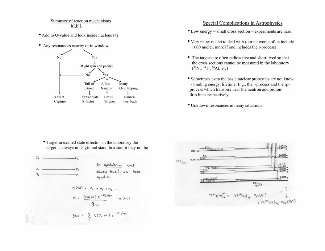
Summary of reaction mechanisms I(j,k)L

•  Add to Q-value and look inside nucleus I+j •  Any resonances nearby or in window

No Yes Right spin and parity? No Yes Tail of A few Many Broad Narrow Overlapping Direct Extrapolate Breit- Hauser- Capture S-factor Wigner Feshbach

Special Complications in Astrophysics •  Low energy = small cross section – experiments are hard. •  Very many nuclei to deal with (our networks often include 1600 nuclei; more if one includes the r-process) •  The targets are often radioactive and short lived so that the cross sections cannot be measured in the laboratory (56Ni, 44Ti, 26Al, etc) •  Sometimes even the basic nuclear properties are not know - binding energy, lifetime. E.g., the r-process and the rp- process which transpire near the neutron and proton- drip lines respectively. •  Unknown resonances in many situations

•  Target in excited state effects – in the laboratory the target is always in its ground state. In a star, it may not be

•  Electron screening Nuclei are always completely ionized – or almost completely ionized at temperature in stars where nuclear fusion occurs. But the density may be sufficiently high that two fusing nuclei do not experience each others full Coulomb repulsion. This is particularly significant in Type Ia supernova ignition.

Electron screening is generally treated in two limiting cases. Weak screening: (Salpeter 1954) The electrical potential of the ion is adjusted to reflect the presence of induced polarization in the background electrons. The characteristic length scale for this screening is the Debye length

           RD=

kT

4πe2ρNAς

⎛⎝⎜

⎞⎠⎟

1/2

ζ = (Zi

2∑ +Zi)Y

i

Clayton 2-238 and discussion before

This is the typical length scale for the clustering of charge in the plasma. Weak screening holds if RD >> nZ

-1/3

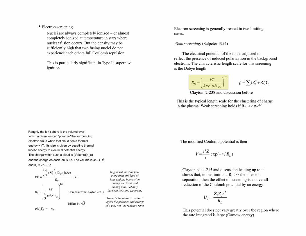
PE =

43πRD

3⎛⎝⎜

⎞⎠⎟ ZnZe( )(Ze)RD

kT

RD ~ kT43πe2Z 2nZ

⎛

⎝

⎜⎜⎜

⎞

⎠

⎟⎟⎟

1/2

Compare with Clayton 2-235

Differs by 3ρNAYZ = nZ

Roughly the ion sphere is the volume overwhich a given ion can "polarize" the surroundingelectron cloud when that cloud has a thermal energy ~kT. Its size is given by equating thermalkinetic energy to electrical potential energy.The charge within such a cloud is (Volume)(ne e)

and the charge on each ion is Ze. The volume is 4/3 πRD3

and ne = ZnZ . So

In general must include more than one kind of

ions and the interaction among electrons and among ions, not only

between ions and electrons,

These “Coulomb correction” affect the pressure and energy of a gas, not just reaction rates

The modified Coulomb potential is then

V =e2Z

rexp(−r / R

D)

Clayton eq. 4-215 and discussion leading up to it shows that, in the limit that RD >> the inter-ion separation, then the effect of screening is an overall reduction of the Coulomb potential by an energy

Uo=ZIZje2

RD

This potential does not vary greatly over the region where the rate integrand is large (Gamow energy)

The leading order term in the screening correction (after considering Mawell Boltzmann average) is then (Clayton 4-221; see also Illiadis 3.143)

f ≈ 1−Uo

kT= 1+0.188ZIZ j ρ

1/2ς 1/2 T6

−3/2

Strong screening: Salpeter (1954); Salpeter and van Horn (1969)

If RD becomes less than the inter-ion spacing, then the screening is no longer weak. Each ion of charge Z is individually screened by Z electrons. The radius of the “ion sphere” is

RZ=

3Z

4πne

⎛⎝⎜

⎞⎠⎟

1/3

i.e.4πR

Z

3

3ne= Z

e.g., the screening for p+p at the solar center is about 5% - Illiadis P 210

U0 << kT

Clayton 2-262, following Salpeter (1954) shows that the total potential energy of the ion sphere, including both the repulsive interaction of the electrons among themselves and the attractive interaction with the ions, is

U = − 910

Ze( )2

RZ

⎛

⎝⎜⎞

⎠⎟=−17.6 Z 5/3 ρYe( )1/3 eV << Gamow energy E0

and the correction factor to the rate is exp(-Uo / kT )>>1 with

−U0 =17.6 ρYe( )1/3 ZI +Z j( )5/3− ZI

5/3 − Z j5/3⎡

⎣⎢⎤⎦⎥ eV (Cla 4-225)

More accurate treatments are available, but this can clearly become very large at high density. See Itoh et al. ApJ, 586, 1436, 2003

Appendix: Barrier Penetration

and Transmission Functions

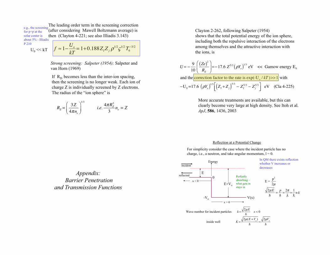
Reflection at a Potential Change

For simplicity consider the case where the incident particle has no charge, i.e., a neutron, and take angular momentum, l = 0.

Energy

E reflected

incident

0

-Vo V(x)

E+Vo x < 0

Perfectly absorbing – what gets in stays in

In QM there exists reflection whether V increases or decreases

E = p

2

2µ

2µE

=

p

=

2π

λ=

1

≡ k

Wave number for incident particles k =2µE

x < 0

inside well K =2µ(E +V

o)

≈

2µVo

x > 0

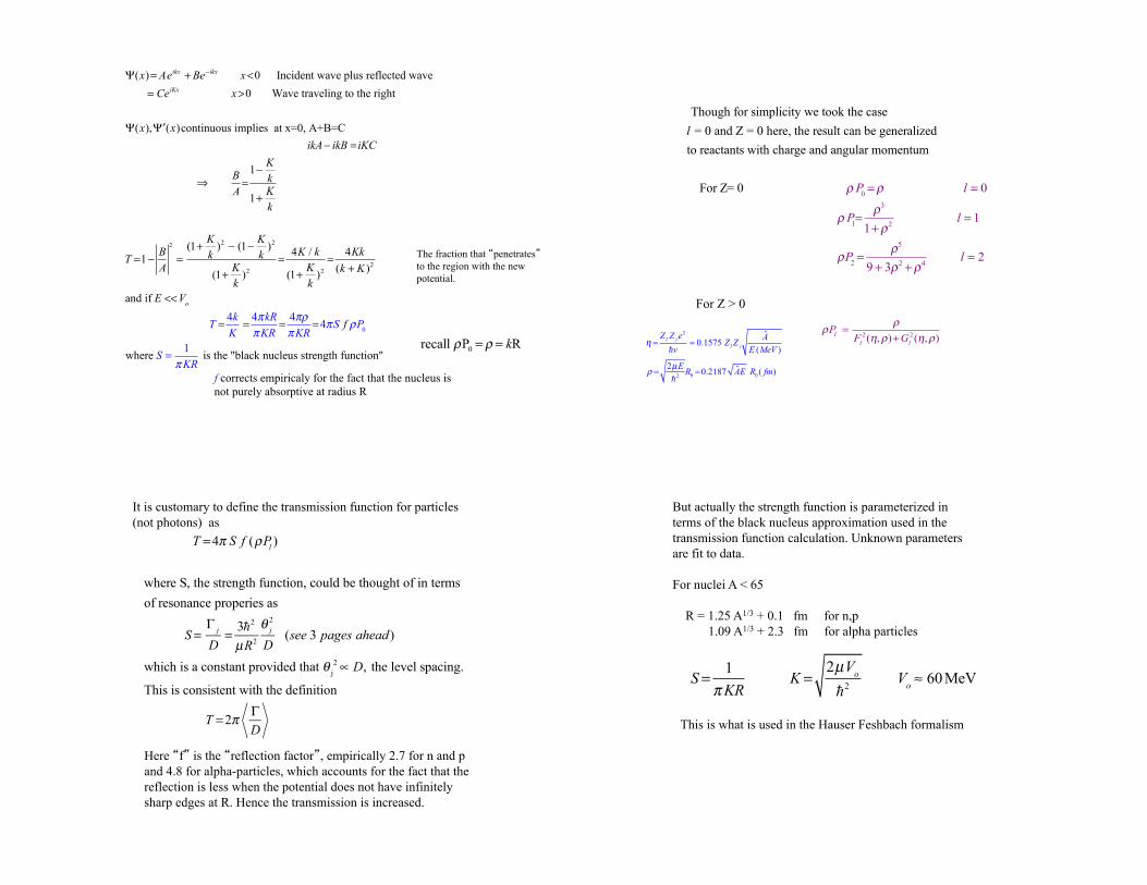
Ψ(x)= Aeikx +Be−ikx x<0 Incident wave plus reflected wave

= CeiKx

x>0 Wave traveling to the right

Ψ(x), ′Ψ (x)continuous implies at x=0, A+B=C

ikA− ikB = iKC

⇒B

A=

1−K

k

1+K

k

T =1−B

A

2

=

(1+K

k)2

− (1−K

k)2

(1+K

k)2

=4K / k

(1+K

k)2

=4Kk

(k + K )2

and if E <<Vo

T =4k

K=

4πkR

πKR=

4πρ

πKR=4πS f ρP

0

where S =1

πKR is the "black nucleus strength function"

The fraction that �penetrates� to the region with the new potential.

0recall P Rkρ ρ= =

f corrects empiricaly for the fact that the nucleus is not purely absorptive at radius R

Though for simplicity we took the case

l = 0 and Z = 0 here, the result can be generalized

to reactants with charge and angular momentum

For Z= 0 ρ P0=ρ l = 0

ρ P1=

ρ3

1+ρ2l = 1

ρP2=

ρ5

9 + 3ρ2+ρ4

l = 2

ρPl=

ρ

Fl

2 (η,ρ)+Gl

2 (η,ρ)

For Z > 0

2

0 02

ˆ0.1575

( )

2 ˆ0.2187 ( )

I j

I j

Z Z e AZ Z

v E MeV

ER AE R fm

η

µρ

= =

= =

It is customary to define the transmission function for particles (not photons) as

T =4π S f (ρPl )

where S, the strength function, could be thought of in termsof resonance properies as

S =Γ j

D= 32

µR2

θ j2

D(see 3 pages ahead)

which is a constant provided that θ j2 ∝ D, the level spacing.

This is consistent with the definition

T =2π ΓD

Here �f� is the �reflection factor�, empirically 2.7 for n and p and 4.8 for alpha-particles, which accounts for the fact that the reflection is less when the potential does not have infinitely sharp edges at R. Hence the transmission is increased.

But actually the strength function is parameterized in terms of the black nucleus approximation used in the transmission function calculation. Unknown parameters are fit to data. For nuclei A < 65 R = 1.25 A1/3 + 0.1 fm for n,p 1.09 A1/3 + 2.3 fm for alpha particles

S =1

πKRK =

2µVo

2

Vo≈ 60MeV

This is what is used in the Hauser Feshbach formalism

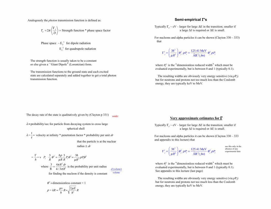
Analogously the photon transmission function is defined as:

3

5

2 Strength function * phase space factor

Phase space E for dipole radiation

E for quadrupole radiation

TD

γ

γ

γ

γ

πΓ

= =

The strength function is usually taken to be a constant or else given a ``Giant Dipole� (Lorentzian) form. The transmission functions to the ground state and each excited state are calculated separately and added together to get a total photon transmission function.

Typically ~ eV – larger for large E in the transition; smaller if a large J is required or E is small. For nucleons and alpha particles it can be shown (Clayton 330 – 333) that

Γj

l=

32

µR2

⎛

⎝⎜⎞

⎠⎟θ

j

2 ρPl=

125.41 MeV

AR2( fm)θ

j

2 ρPl

where j2 is the �dimensionless reduced width� which must be

evaluated experimentally, but is between 0 and 1 (typically 0.1). The resulting widths are obviously very energy sensitive (via Pl) but for neutrons and protons not too much less than the Coulomb energy, they are typically keV to MeV.

Semi-empirical ’s

The decay rate of the state is qualitatively given by (Clayton p 331)

λ ≡probability/sec for particle from decaying system to cross large

spherical shell

λ =1

τ= velocity at infinity * penetration factor * probability per unit dr

that the particle is at the nuclear

radius ± dr

= Γ

= v P

l

3

Rθ2=ρ

µR

3

RPlθ2=3

µR2ρP

lθ 2

where 3

R=4πR

2dr

4 / 3πR3

is the probability per unit radius

for finding the nucleon if the density is constant

θ 2 =dimensionless constant < 1

ρ = kR =µv

R=

2µE

2R

( )d volume

volume

aside:

Typically ~ eV – larger for large E in the transition; smaller if a large J is required or E is small. For nucleons and alpha particles it can be shown (Clayton 330 – 333 and appendix to this lecture) that

Γj

l=

32

µR2

⎛

⎝⎜⎞

⎠⎟θ

j

2 ρPl=

125.41 MeV

AR2( fm)θ

j

2 ρPl

where j2 is the �dimensionless reduced width� which must be

evaluated experimentally, but is between 0 and 1 (typically 0.1). See appendix to this lecture (last page) The resulting widths are obviously very energy sensitive (via Pl) but for neutrons and protons not too much less than the Coulomb energy, they are typically keV to MeV.

Very approximate estimates for '

use this only in the absence of any experimental data