2.019 Design of Ocean Systems

Lecture 6

Seakeeping (II)

February 21, 2011

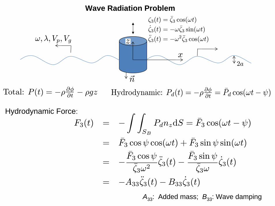
Wave Radiation Problem

ζ3(t) = ζ3 cos(ωt)

ζ3(t) = −ω ζ3 sin(ωt) ¨ ζ3(t) = −ω2 ζ3 cos(ωt)

x

zω,λ, Vp, Vg

2a

~n

Total: P (t) = −ρ ∂φ − ρgz Hydrodynamic: Pd(t) = −ρ ∂φ = Pd cos(ωt− ψ)∂t ∂t

Hydrodynamic Force: Z Z ¯F3(t) = −

SB

PdnzdS = F3 cos(ωt− ψ)

¯ ¯= F3 cos ψ cos(ωt) + F3 sin ψ sin(ωt) ¯ ¯F3 cos ψ F3 sin ψ

= − ζ3ω2

ζ 3(t) −

ζ3ωζ 3(t)¯ ¯

= −A33ζ 3(t) − B33ζ

3(t)

A33: Added mass; B33: Wave damping

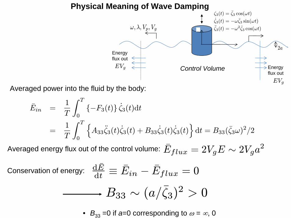
Physical Meaning of Wave Damping ζ3(t) =

ω,λ, Vp, Vg z ζ 3(t) = −ω2ζ3 cos(ωt)

x 2a

Energy flux out EVg Control Volume Energy

flux out

Averaged power into the fluid by the body:

ζ3 cos(ωt)

ζ3(t) = −ω ζ3 sin(ωt)

EVg

Z T

Ein =1 {−F3(t)} ζ

3(t)dt T 0 Z T n o

=1

A33ζ 3(t)ζ

3(t) + B33ζ 3(t)ζ

3(t) dt = B33(ζ3ω)2/2

T 0

Averaged energy flux out of the control volume: Eflux = 2VgE ∼ 2Vga 2

dEConservation of energy: ≡ Ein − Eflux = 0dt

B33 ∼ (a/ζ3)2 > 0

• B33 =0 if a=0 corresponding to ω = ∞, 0

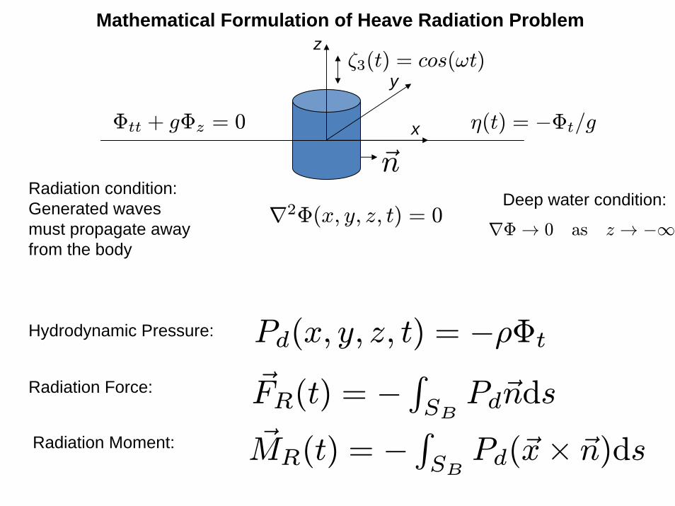
Mathematical Formulation of Heave Radiation Problem z

ζ3(t) = cos(ωt) y

Φtt + gΦz = 0 η(t) = −Φt/gx

~n Radiation condition: Generated waves must propagate away from the body

Hydrodynamic Pressure:

Radiation Force:

Radiation Moment:

Deep water condition: ∇2Φ(x, y, z, t) = 0 ∇Φ → z → −∞ 0 as

Pd(x, y, z, t) = −ρΦt R F~R(t) = − Pd ~ndsSBR M~R(t) = −

SB Pd(~x × ~n)ds

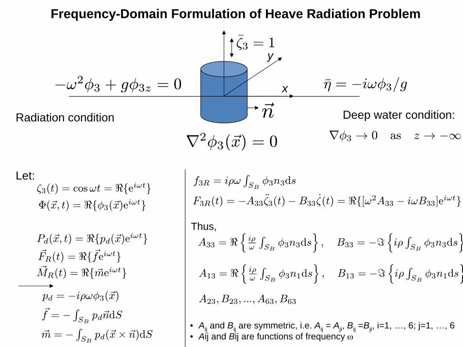
Frequency-Domain Formulation of Heave Radiation Problem

¯ζ3 = 1 y

−ω2φ3 + gφ3z = 0 η = −iωφ3/gx

Radiation condition ~n Deep water condition:

Let: ζ3(t) = cosωt = <{eiωt} Φ(~x, t) = <{φ3(~x)eiωt}η(x, y, t) = <{η(x, y)eiωt}

Pd(~x, t) = <{pd(~x)eiωt} F~R( f~eiωt

M~R(

t) = <{

~ iω

}tmet) = <{ }

pd = −iρωφ3(~x) R f~ = −

SB pd ~ndS R

~ = − SB pd(~ × ~n)dSm x

∇2φ3(~x) = 0 ∇φ3 → 0 as z → −∞

R f3R = iρω

SB φ3n3ds

F3R(t) = −A33ζ 3(t)− B33ζ(t) = <{[ω2A33 − iωB33]eiωt}

Thus, n R o n R o A33 = < i

ωρ φ3n3ds , B33 = −= iρ φ3n3dsSB SB n R o n R o

A13 = < iωρ

SB φ3n1ds , B13 = −= iρ

SB φ3n1ds

A23, B23, ..., A63, B63

• Aij and Bij are symmetric, i.e. Aij = Aji, Bij =Bji, i=1, …, 6; j=1, …, 6 • Aij and Bij are functions of frequency ω

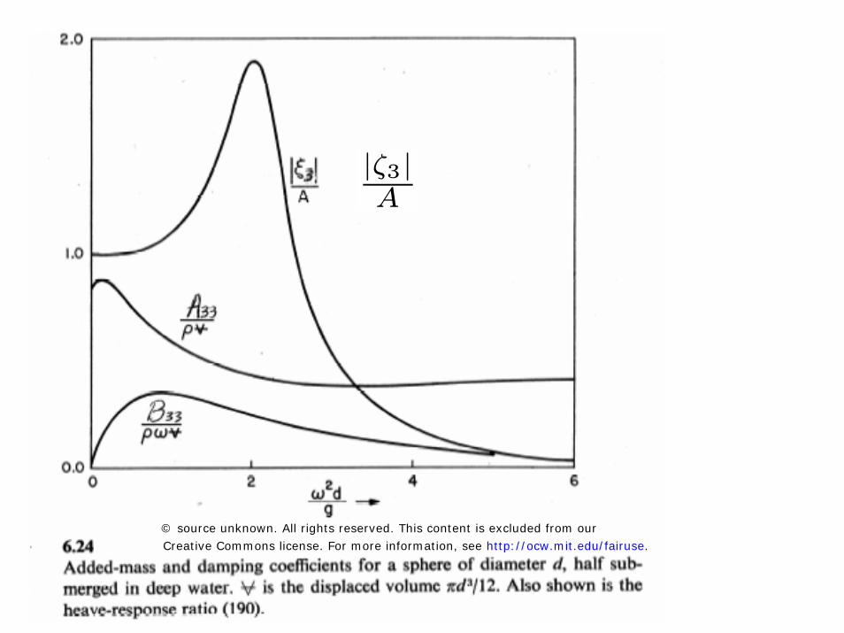
|ζ3 |A

© source unknown. All rights reserved. This content is excluded from ourCreative Commons license. For more information, see http://ocw.mit.edu/fairuse.

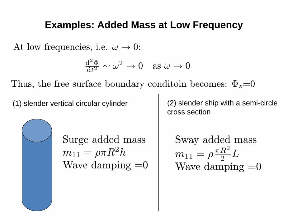
Examples: Added Mass at Low Frequency

At low frequencies, i.e. ω 0:→

d2 Φ 0 as ω 0dt2 ∼ ω2 → →

Thus, the free surface boundary conditoin becomes: Φz=0

(1) slender vertical circular cylinder

Surge added mass m11 = ρπR2h Wave damping =0

(2) slender ship with a semi-circle cross section

Sway added mass= ρ πR

2m11 2 L Wave damping =0

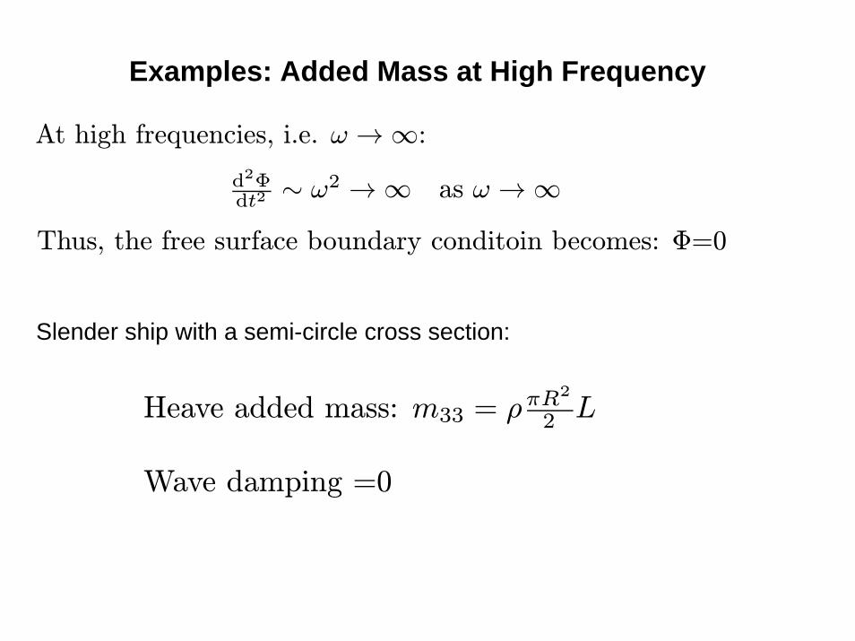
Examples: Added Mass at High Frequency

At high frequencies, i.e. ω →∞: d2 Φ dt2 ∼ ω2 →∞ as ω →∞

Thus, the free surface boundary conditoin becomes: Φ=0

Slender ship with a semi-circle cross section:

= ρ πR2

Heave added mass: m33 2 L

Wave damping =0

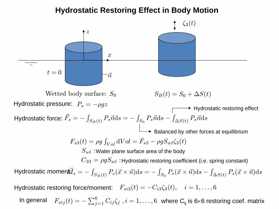
Hydrostatic Restoring Effect in Body Motion ζ3(t)

Wetted body surface: S0 SB(t) = S0 + ∆S(t)

~n

z

x

t = 0

Hydrostatic pressure: Ps = −ρgz Hydrostatic restoring effect R R R

Hydrostatic force: F~s = − SB (t)

Ps ~nds = − S0 Ps ~nds−

∆S(t) Ps ~nds

Balanced by other forces at equilibrium R ¯Fs3(t) = ρg dV ol = Fs3 − ρgSwlζ3(t)V ol

Swl :Water plane surface area of the body C33 = ρgSwl :Hydrostatic restoring coefficient (i.e. spring constant) R R R

~Hydrostatic moment:Ms = − SB (t)

Ps(~x× ~n)ds = − Ps(~x× ~n)ds− ∆S(t) Ps(~x× ~n)ds

S0

Hydrostatic restoring force/moment: Fsi3(t) = −Ci3ζ3(t), i = 1, . . . , 6

In general Fsij(t) = − P6 Cijζj , i = 1, . . . , 6 where Cij is 6×6 restoring coef. matrixj=1

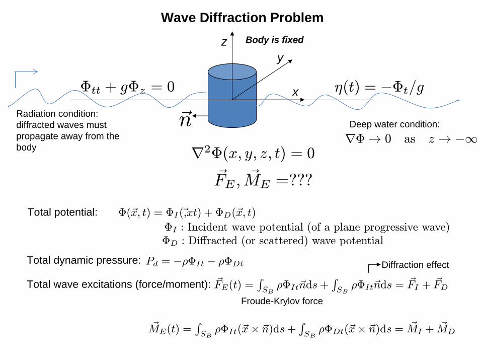
Wave Diffraction Problem

x

y

Φtt + gΦz = 0 η(t) = −Φt/g Radiation condition: diffracted waves must Deep water condition:~n

z Body is fixed

propagate away from the 0 as body ∇2Φ(x, y, z, t) = 0

∇Φ → z → −∞

F~E , M~E =???

Total potential: Φ(~x, t) = ΦI(~,xt) + ΦD(~x, t)ΦI : Incident wave potential (of a plane progressive wave)ΦD : Diffracted (or scattered) wave potential

Total dynamic pressure: Pd = −ρΦIt − ρΦDt Diffraction effect R R ~ ~ ~Total wave excitations (force/moment): FE(t) = ρΦIt ~nds + ρΦIt ~nds = FI + FDSB SB

Froude-Krylov force R R M~E(t) =

SB ρΦIt(~x × ~n)ds +

SB ρΦDt(~x × ~n)ds = M~ I + M~D

wave:

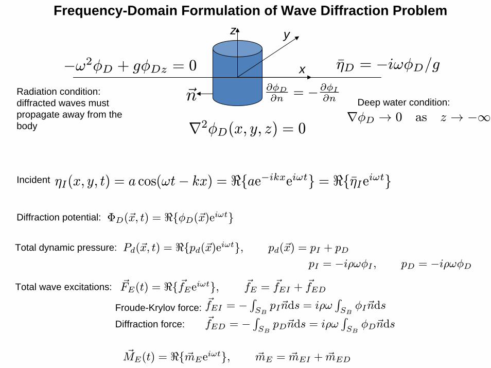
Frequency-Domain Formulation of Wave Diffraction Problem z y

−ω2φD + gφDz = 0 ηD = −iωφD/gx

Radiation condition: ∂φD ∂φI

diffracted waves must ~n ∂n = − ∂n Deep water condition: propagate away from the φD 0 as body ∇2φD(x, y, z) = 0

∇ → z → −∞

Incident ηI (x, y, t) = a cos(ωt − kx) = <{ae−ikxeiωt} = <{ηI eiωt}

} = <{φIe }ΦI(~x, t) = −(ga/ω) sin(ωt − kx)ekz = <{(−iga/ω)ekz−ikxeiωt iωt

Diffraction potential: ΦD(~x, t) = <{φD(~x)eiωt}

Total dynamic pressure: Pd(~x, t) = <{pd(~x)eiωt}, pd(~x) = pI + pD

pI = −iρωφI , pD = −iρωφD

Total wave excitations: F~E(t) = <{f~Eeiωt}, f~E = f~EI + f~ED R R Froude-Krylov force: f~EI = −

SB pI ~nds = iρω

SB φI ~nds R R

Diffraction force: f~ED = − SB pD ~nds = iρω

SB φD ~nds

~ ~ = ~ ~M~E(t) = <{mEeiωt}, mE mEI +mED

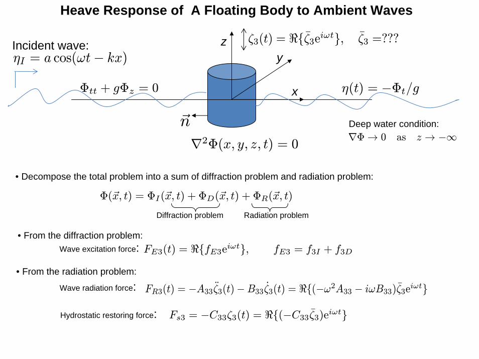
Heave Response of A Floating Body to Ambient Waves

x

y

Φtt + gΦz = 0 η(t) = −Φt/g

Deep water condition:

z

~n

ζ3(t) = <{ ζ3eiωt}, ζ3 =???

ηI = a cos(ωt − kx) Incident wave:

x, t) + ΦD(~x, t) + ΦR(~x, t)

Diffraction problem Radiation problem

∇2Φ(x, y, z, t) = 0 ∇Φ → 0 as z → −∞

• Decompose the total problem into a sum of diffraction problem and radiation problem:

Φ(~x, t) = ΦI (~

• From the diffraction problem: Wave excitation force: FE3(t) = <{fE3eiωt}, fE3 = f3I + f3D

• From the radiation problem:

Wave radiation force: FR3(t) = −A33ζ 3(t)− B33ζ

3(t) = <{(−ω2A33 − iωB33)ζ3eiωt}

Hydrostatic restoring force: Fs3 = −C33ζ3(t) = <{(−C33ζ3)eiωt}

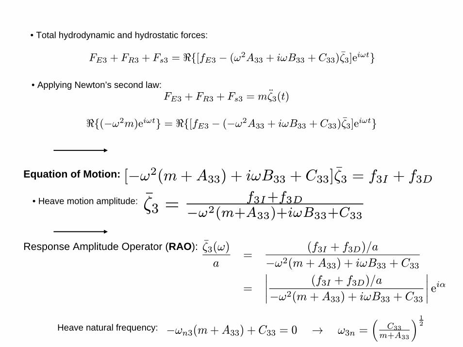
• Total hydrodynamic and hydrostatic forces:

FE3 + FR3 + Fs3 = <{[fE3 − (ω2A33 + iωB33 + C33)ζ3]eiωt}

• Applying Newton’s second law: ¨ FE3 + FR3 + Fs3 = mζ3(t)

<{(−ω2m)eiωt} = <{[fE3 − (−ω2A33 + iωB33 + C33)ζ3]eiωt}

Equation of Motion: [−ω2(m+A33) + iωB33 + C33]ζ3 = f3I + f3D

• Heave motion amplitude: ζ3 = f3I +f3D−ω2(m+A33)+iωB33+C33

¯

Response Amplitude Operator (RAO): ζ3(ω) (f3I + f3D)/a = −ω2(a m +A33) + iωB33 + C33 ¯

(f3I + f3D)/a iα = e−ω2(m +A33) + iωB33 + C33´³

Heave natural frequency: C33−ωn3(m +A33) + C33 = 0 → ω3n = m+A33

1 2

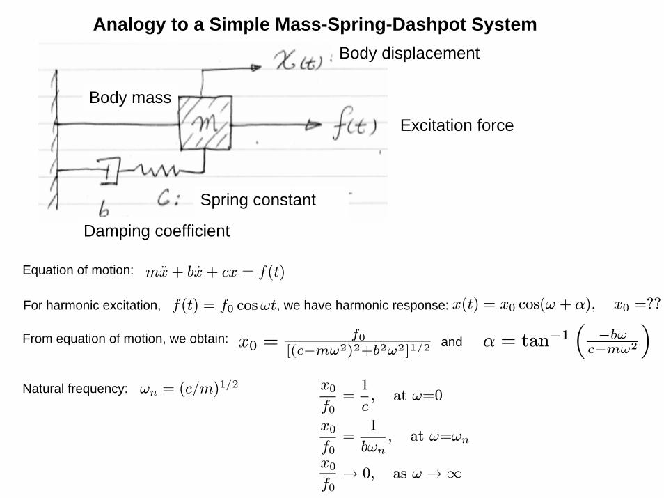
Analogy to a Simple Mass-Spring-Dashpot System Body displacement

Spring constant

Excitation force

Damping coefficient

Body mass

Equation of motion: mx+ bx+ cx = f(t)

For harmonic excitation, f(t) = f0 cos ωt, we have harmonic response: x(t) = x0 cos(ω + α), x0 =??³ ´ From equation of motion, we obtain: = f0 and α = tan−1 −bω x0 [(c−mω2)2+b2ω2]1/2 c−mω2

Natural frequency: ωn = (c/m)1/2 x0

=1 , at ω=0

f0 c x0 1 = , at ω=ωn

f0 bωn x0

f0 → 0, as ω →∞

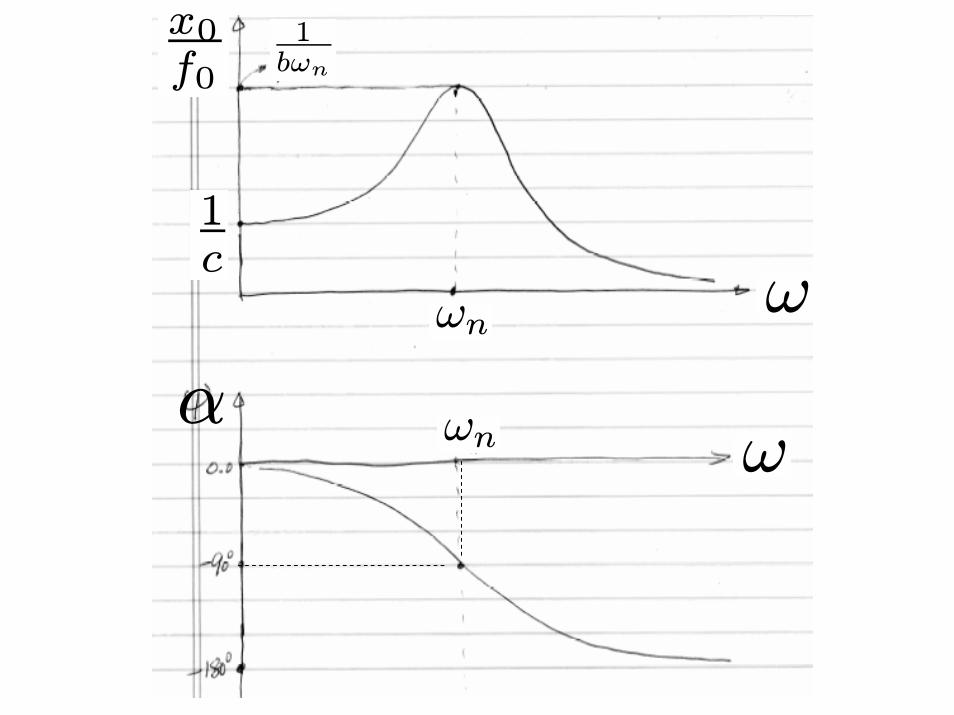
x0 f0

1 bωn

1 c

α ωn

ωn

ω

ω

MIT OpenCourseWarehttp://ocw.mit.edu

2.019 Design of Ocean Systems Spring 2011

For information about citing these materials or our Terms of Use, visit: http://ocw.mit.edu/terms.