RADYN

Mats Carlsson

Institute of Theoretical Astrophysics, Univ Oslo

Wrocław, October 31 2016

(with much input from Joel Allred, NASA/GSFC)

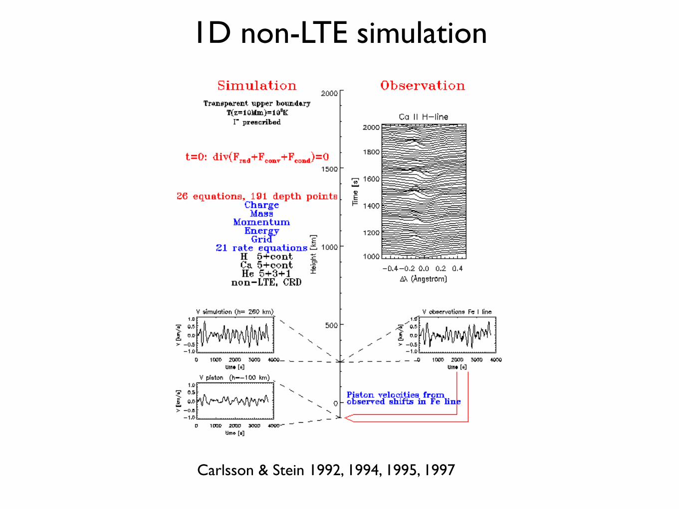
1D non-LTE simulation

Carlsson & Stein 1992, 1994, 1995, 1997

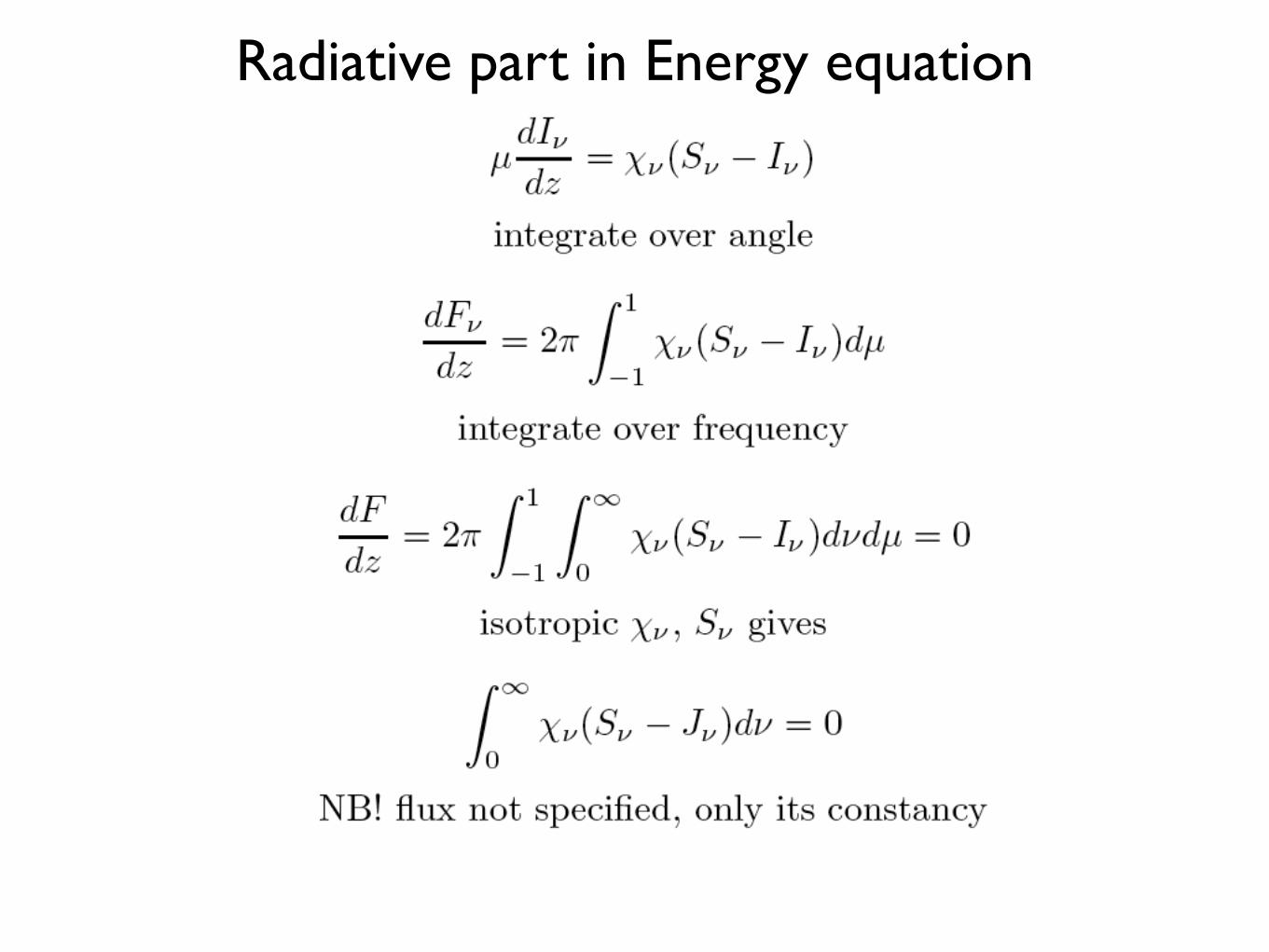
Radiative part in Energy equation

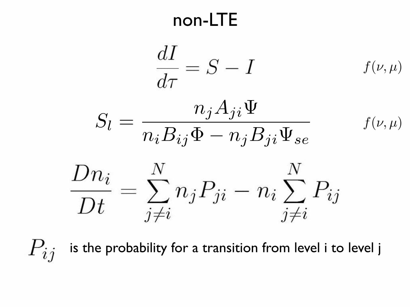
non-LTE

is the probability for a transition from level i to level j

Sl =njAjiΨ

niBijΦ − njBjiΨse

f(ν, µ)

f(ν, µ)

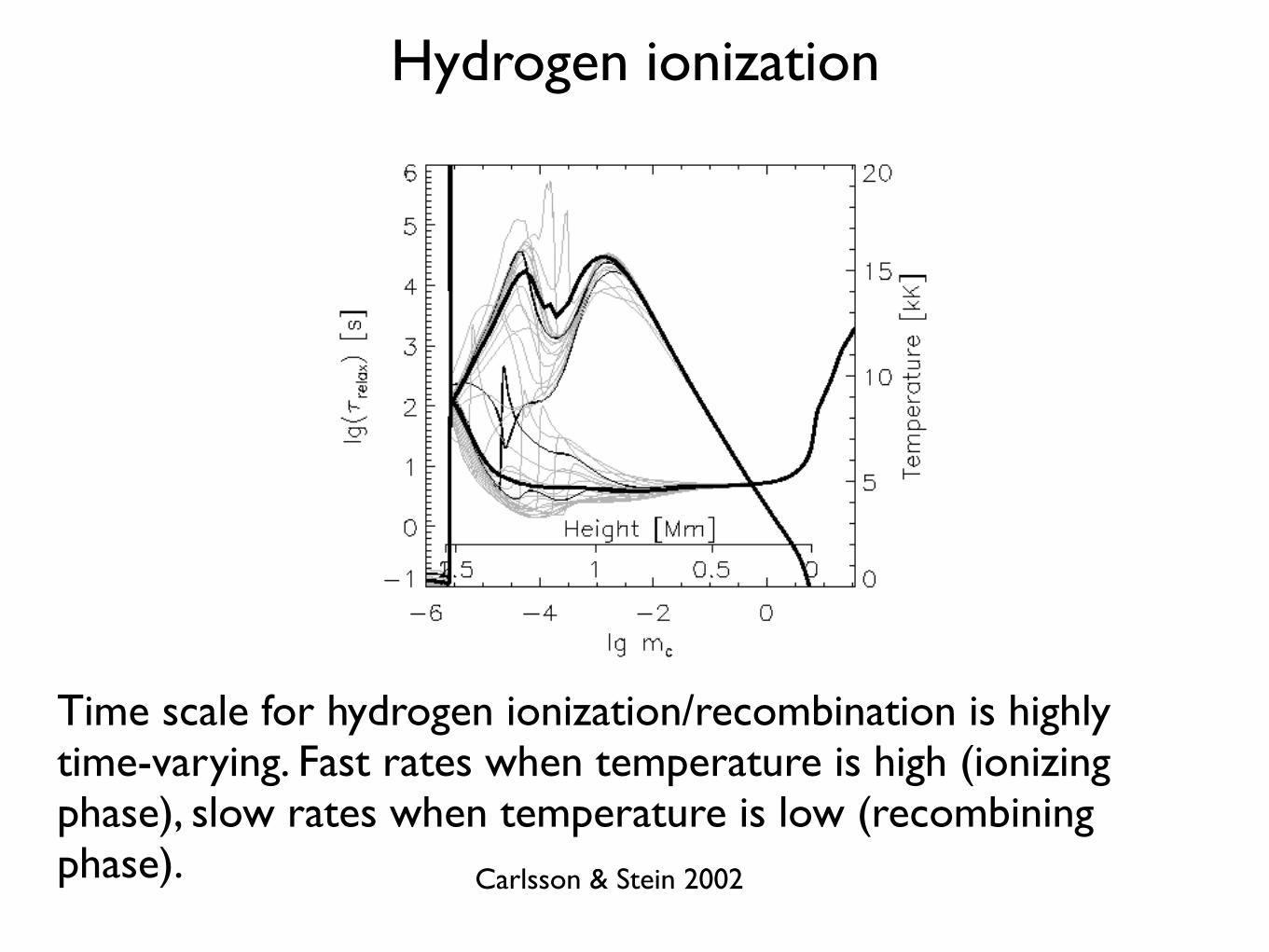
Hydrogen ionization

Time scale for hydrogen ionization/recombination is highly time-varying. Fast rates when temperature is high (ionizing phase), slow rates when temperature is low (recombining phase). Carlsson & Stein 2002

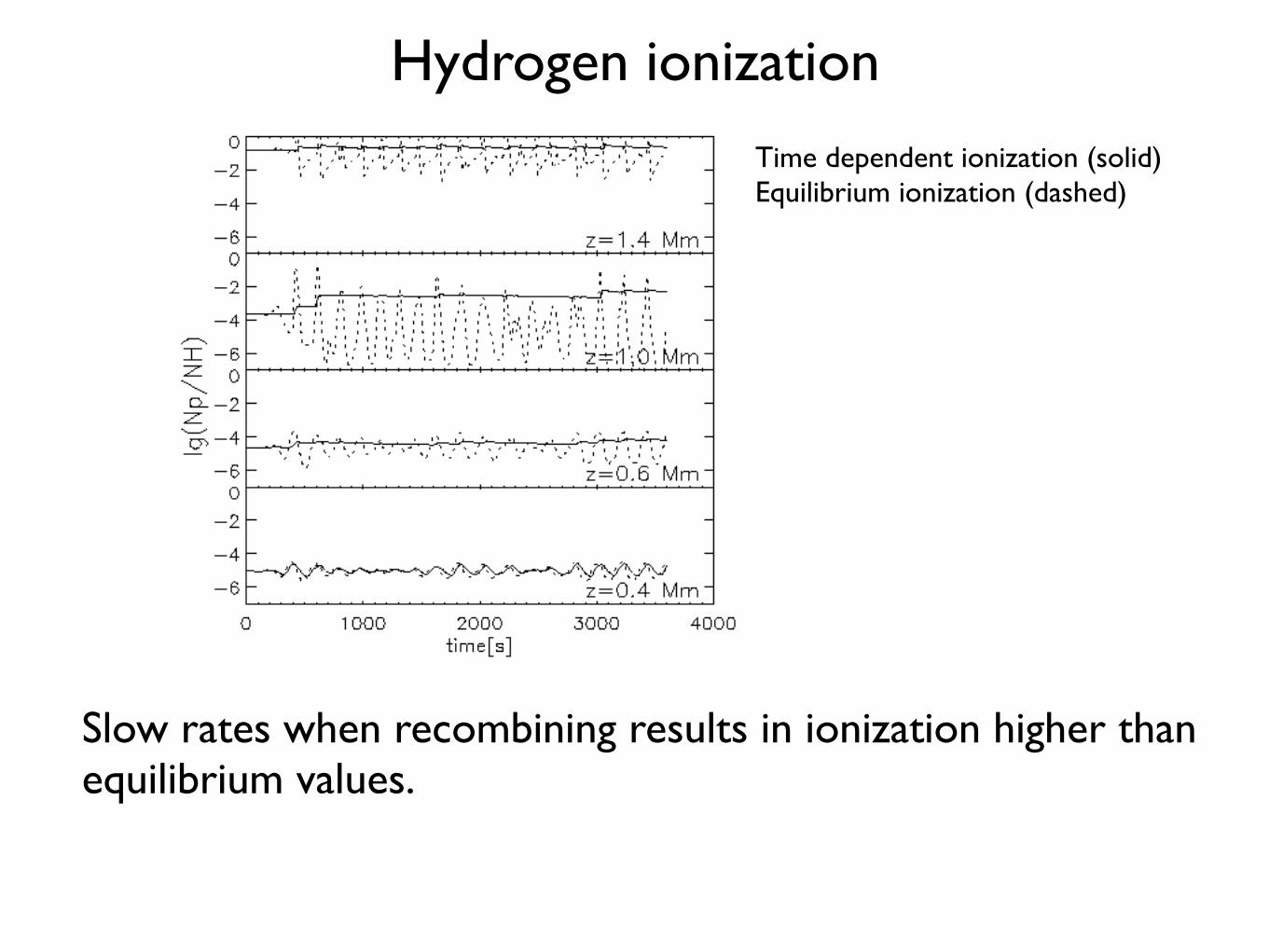
Hydrogen ionization

Slow rates when recombining results in ionization higher than equilibrium values.

Time dependent ionization (solid)Equilibrium ionization (dashed)

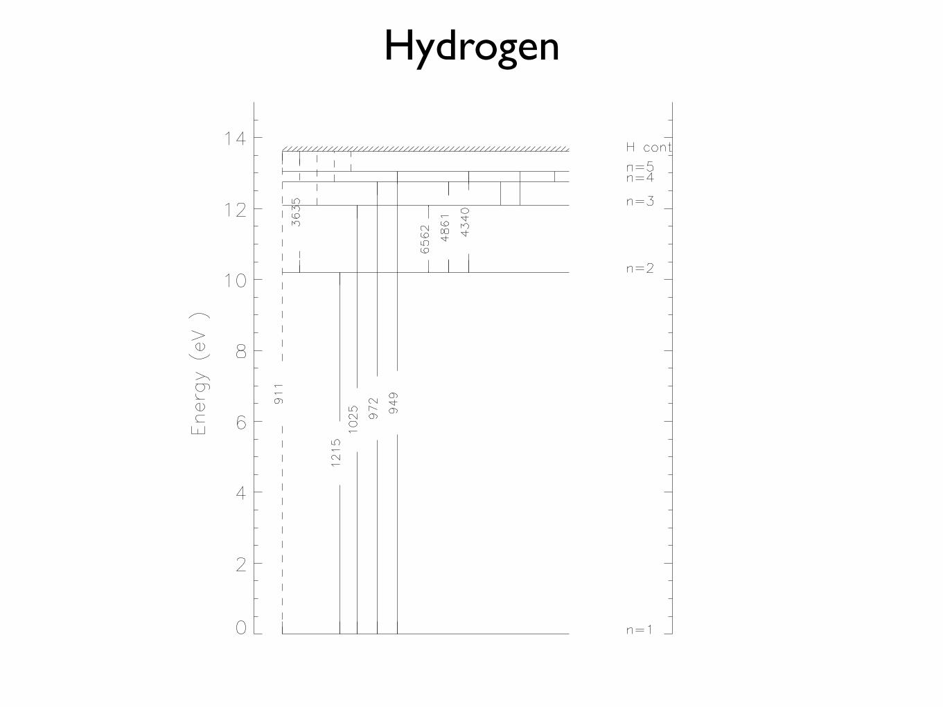
Hydrogen

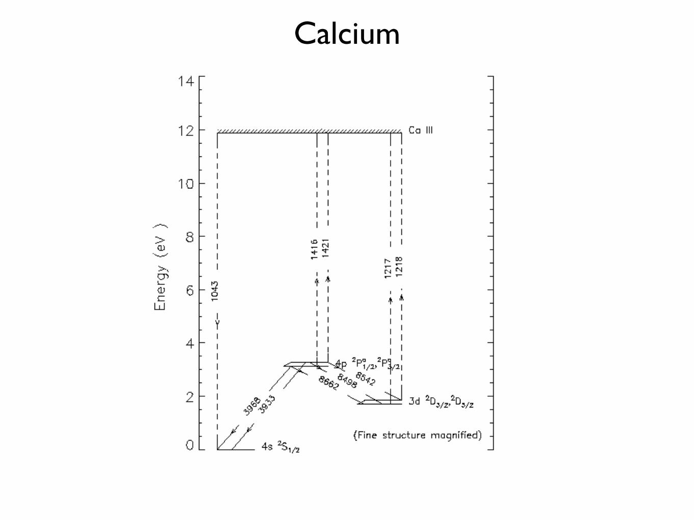
Calcium

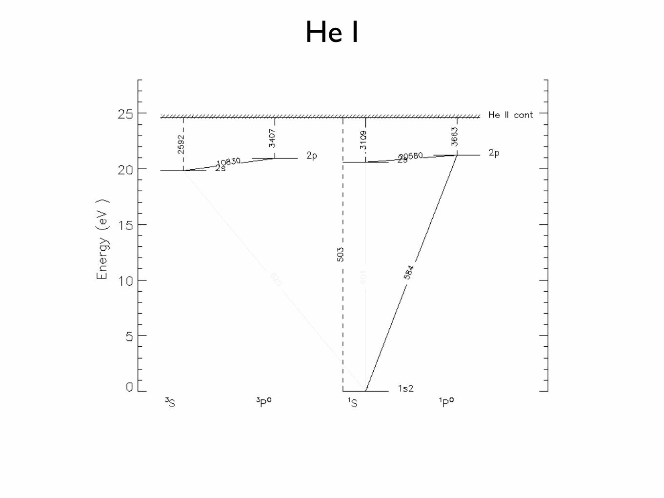
He I

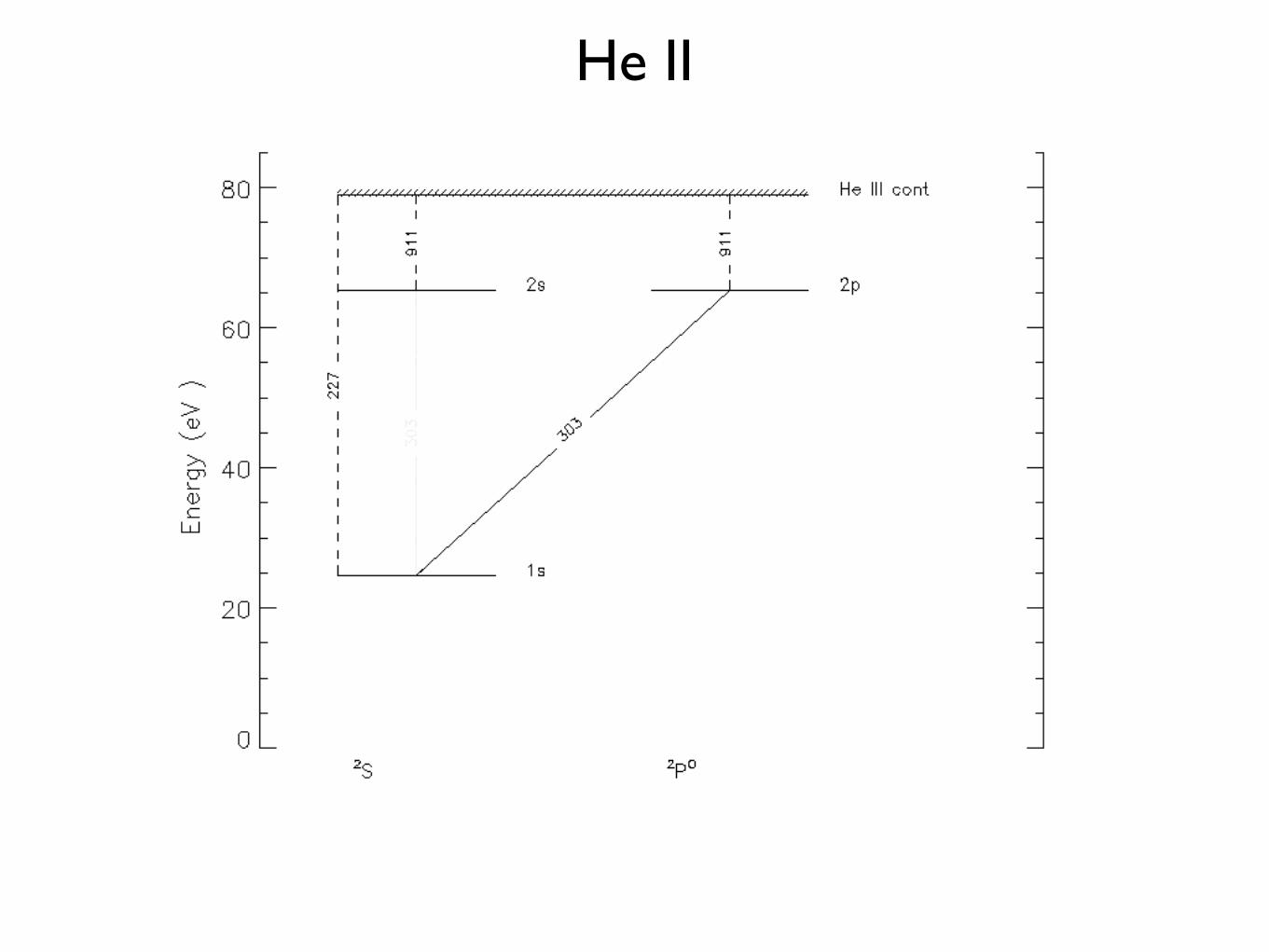
He II

4 Allred, Kowalski, and Carlsson

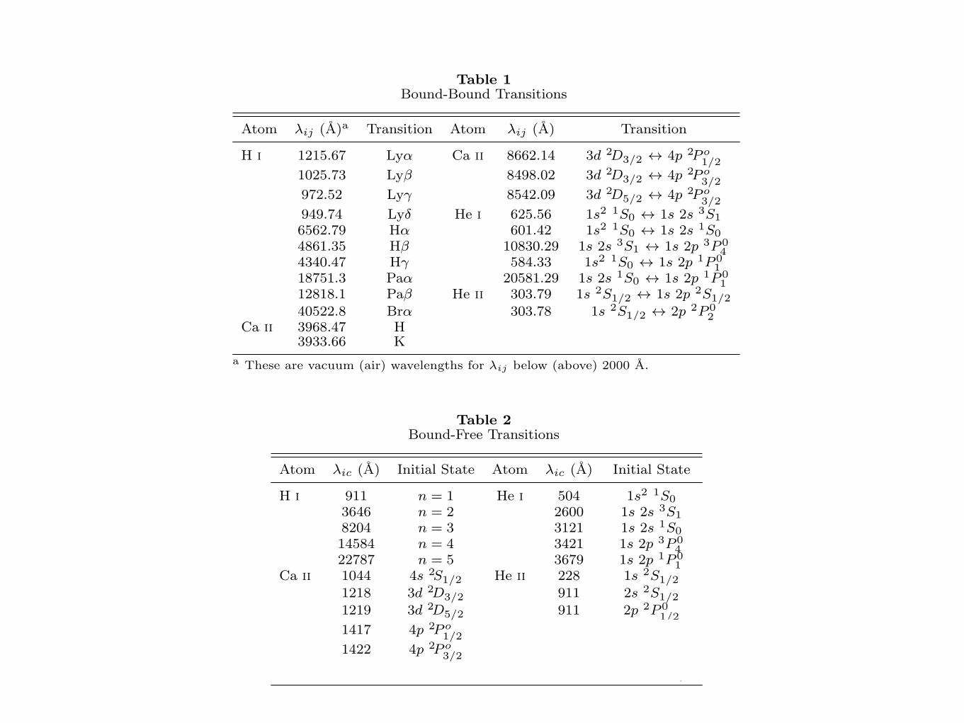
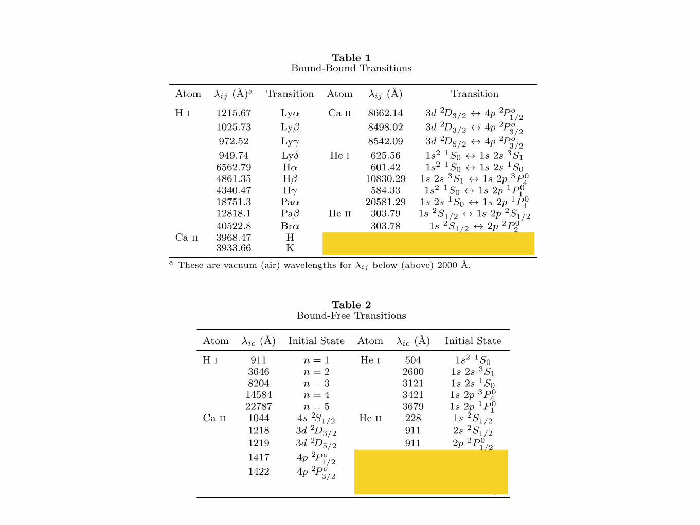
Table 1Bound-Bound Transitions

Atom λij (A)a Transition Atom λij (A) Transition

H i 1215.67 Lyα Ca ii 8662.14 3d 2D3/2 ↔ 4p 2P o1/2

1025.73 Lyβ 8498.02 3d 2D3/2 ↔ 4p 2P o3/2

972.52 Lyγ 8542.09 3d 2D5/2 ↔ 4p 2P o3/2

949.74 Lyδ He i 625.56 1s2 1S0 ↔ 1s 2s 3S1

6562.79 Hα 601.42 1s2 1S0 ↔ 1s 2s 1S0

4861.35 Hβ 10830.29 1s 2s 3S1 ↔ 1s 2p 3P 04

4340.47 Hγ 584.33 1s2 1S0 ↔ 1s 2p 1P 01

18751.3 Paα 20581.29 1s 2s 1S0 ↔ 1s 2p 1P 01

12818.1 Paβ He ii 303.79 1s 2S1/2 ↔ 1s 2p 2S1/2

40522.8 Brα 303.78 1s 2S1/2 ↔ 2p 2P 02

Ca ii 3968.47 H Mg ii 2802.70 h3933.66 K 2795.53 k

a These are vacuum (air) wavelengths for λij below (above) 2000 A.

Table 2Bound-Free Transitions

Atom λic (A) Initial State Atom λic (A) Initial State

H i 911 n = 1 He i 504 1s2 1S0

3646 n = 2 2600 1s 2s 3S1

8204 n = 3 3121 1s 2s 1S0

14584 n = 4 3421 1s 2p 3P 04

22787 n = 5 3679 1s 2p 1P 01

Ca ii 1044 4s 2S1/2 He ii 228 1s 2S1/2

1218 3d 2D3/2 911 2s 2S1/2

1219 3d 2D5/2 911 2p 2P 01/2

1417 4p 2P o1/2 Mg ii 824 2p6 3s 2S1/2

1422 4p 2P o3/2 1168 2p6 4p 2P 0

1/2

1169 2p6 4p 2P 03/2

flux, the region of the chromosphere where the Ca ii Hline center forms is cooler resulting in an overabundanceof ground state ions and an overall absorption profile.For both XEUV backwarming techniques, the Ca ii Hline has a central reversal peaking in the near wings.The technique of A05 predicts more flux in the centralreversal than our technique. Since their technique doesnot include direct photoionizations by the XEUV flux,it predicts an overabundance of Ca ii relative to Ca iiiions, and hence an increased flux in the Ca ii H centralreversal.

2.4. Opacity

Of course, there are many continuum transitions notincluded in Table 2. The contribution to the opacity dueto these transitions is treated using the opacity packageof Gustafsson (1973). This package constructs opacity asa function of temperature, density and frequency assum-ing that these transitions are in LTE. These are includedas a background opacity source in the detailed calcula-tions of the transitions listed in Table 2.

2.5. Line Broadening

Observations of flares on dMe stars (Hawley & Pet-tersen 1991; Hawley et al. 2003; Kowalski et al. 2010) andthe Sun (Johns-Krull et al. 1997) have shown that the hy-drogen Balmer lines can become extremely broadened.These authors speculate the cause to be Stark broaden-ing, and that conclusion is supported by the models of

10−5 10−4 10−3 10−2 10−1 100 101

Column Mass (g cm−2)

103

104

105

Tem

pera

ture

(K)

w/ XEUV backwarmingw/o XEUV backwarming

using technique of Allred et al. (2005)

Figure 2. The temperature as a function of column mass for loopmodels generated using the XEUV backwarming method describedhere (black), using the XEUV technique of A05 (green) and withoutXEUV backwarming (red).

Allred et al. (2006) and Paulson et al. (2006). In orderto test this against other possible sources of broadening,such as thermal or turbulent broadening, we have im-plemented a technique in RADYN to model Stark linebroadening. The amount of Stark broadening dependsupon the local electron density. Therefore, determiningit can further constrain models of flaring stellar atmo-spheres.That the orbital angular momentum states of hydro-

gen labeled by the quantum number, l, are not degen-

4 Allred, Kowalski, and Carlsson

Table 1Bound-Bound Transitions

Atom λij (A)a Transition Atom λij (A) Transition

H i 1215.67 Lyα Ca ii 8662.14 3d 2D3/2 ↔ 4p 2P o1/2

1025.73 Lyβ 8498.02 3d 2D3/2 ↔ 4p 2P o3/2

972.52 Lyγ 8542.09 3d 2D5/2 ↔ 4p 2P o3/2

949.74 Lyδ He i 625.56 1s2 1S0 ↔ 1s 2s 3S1

6562.79 Hα 601.42 1s2 1S0 ↔ 1s 2s 1S0

4861.35 Hβ 10830.29 1s 2s 3S1 ↔ 1s 2p 3P 04

4340.47 Hγ 584.33 1s2 1S0 ↔ 1s 2p 1P 01

18751.3 Paα 20581.29 1s 2s 1S0 ↔ 1s 2p 1P 01

12818.1 Paβ He ii 303.79 1s 2S1/2 ↔ 1s 2p 2S1/2

40522.8 Brα 303.78 1s 2S1/2 ↔ 2p 2P 02

Ca ii 3968.47 H Mg ii 2802.70 h3933.66 K 2795.53 k

a These are vacuum (air) wavelengths for λij below (above) 2000 A.

Table 2Bound-Free Transitions

Atom λic (A) Initial State Atom λic (A) Initial State

H i 911 n = 1 He i 504 1s2 1S0

3646 n = 2 2600 1s 2s 3S1

8204 n = 3 3121 1s 2s 1S0

14584 n = 4 3421 1s 2p 3P 04

22787 n = 5 3679 1s 2p 1P 01

Ca ii 1044 4s 2S1/2 He ii 228 1s 2S1/2

1218 3d 2D3/2 911 2s 2S1/2

1219 3d 2D5/2 911 2p 2P 01/2

1417 4p 2P o1/2 Mg ii 824 2p6 3s 2S1/2

1422 4p 2P o3/2 1168 2p6 4p 2P 0

1/2

1169 2p6 4p 2P 03/2

flux, the region of the chromosphere where the Ca ii Hline center forms is cooler resulting in an overabundanceof ground state ions and an overall absorption profile.For both XEUV backwarming techniques, the Ca ii Hline has a central reversal peaking in the near wings.The technique of A05 predicts more flux in the centralreversal than our technique. Since their technique doesnot include direct photoionizations by the XEUV flux,it predicts an overabundance of Ca ii relative to Ca iiiions, and hence an increased flux in the Ca ii H centralreversal.

2.4. Opacity

Of course, there are many continuum transitions notincluded in Table 2. The contribution to the opacity dueto these transitions is treated using the opacity packageof Gustafsson (1973). This package constructs opacity asa function of temperature, density and frequency assum-ing that these transitions are in LTE. These are includedas a background opacity source in the detailed calcula-tions of the transitions listed in Table 2.

2.5. Line Broadening

Observations of flares on dMe stars (Hawley & Pet-tersen 1991; Hawley et al. 2003; Kowalski et al. 2010) andthe Sun (Johns-Krull et al. 1997) have shown that the hy-drogen Balmer lines can become extremely broadened.These authors speculate the cause to be Stark broaden-ing, and that conclusion is supported by the models of

10−5 10−4 10−3 10−2 10−1 100 101

Column Mass (g cm−2)

103

104

105

Tem

pera

ture

(K)

w/ XEUV backwarmingw/o XEUV backwarming

using technique of Allred et al. (2005)

Figure 2. The temperature as a function of column mass for loopmodels generated using the XEUV backwarming method describedhere (black), using the XEUV technique of A05 (green) and withoutXEUV backwarming (red).

Allred et al. (2006) and Paulson et al. (2006). In orderto test this against other possible sources of broadening,such as thermal or turbulent broadening, we have im-plemented a technique in RADYN to model Stark linebroadening. The amount of Stark broadening dependsupon the local electron density. Therefore, determiningit can further constrain models of flaring stellar atmo-spheres.That the orbital angular momentum states of hydro-

gen labeled by the quantum number, l, are not degen-

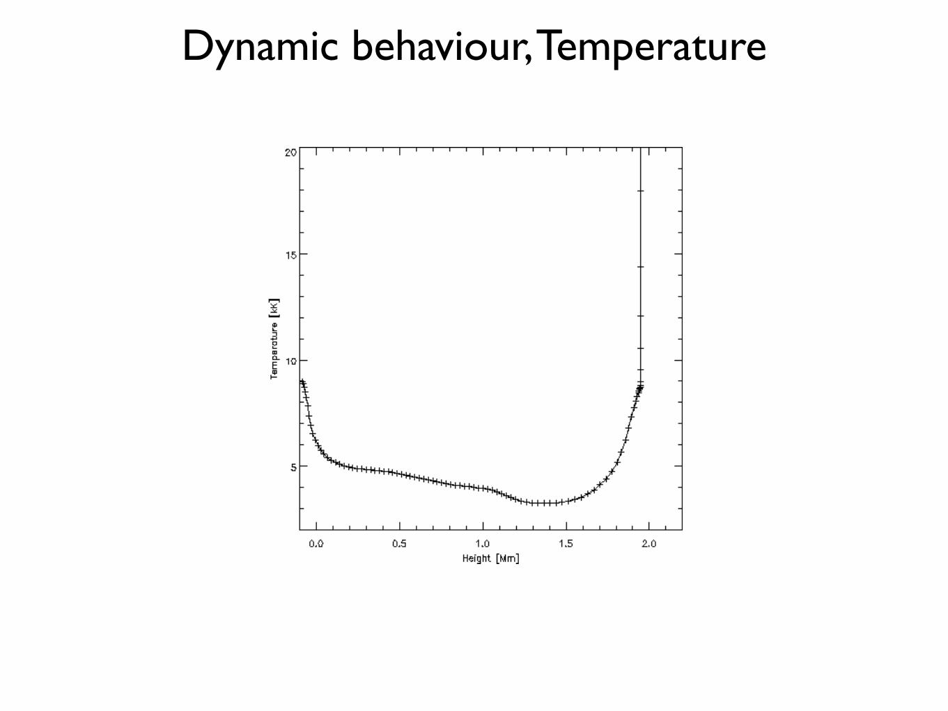
Dynamic behaviour, Temperature

Dynamic behaviour, Temperature

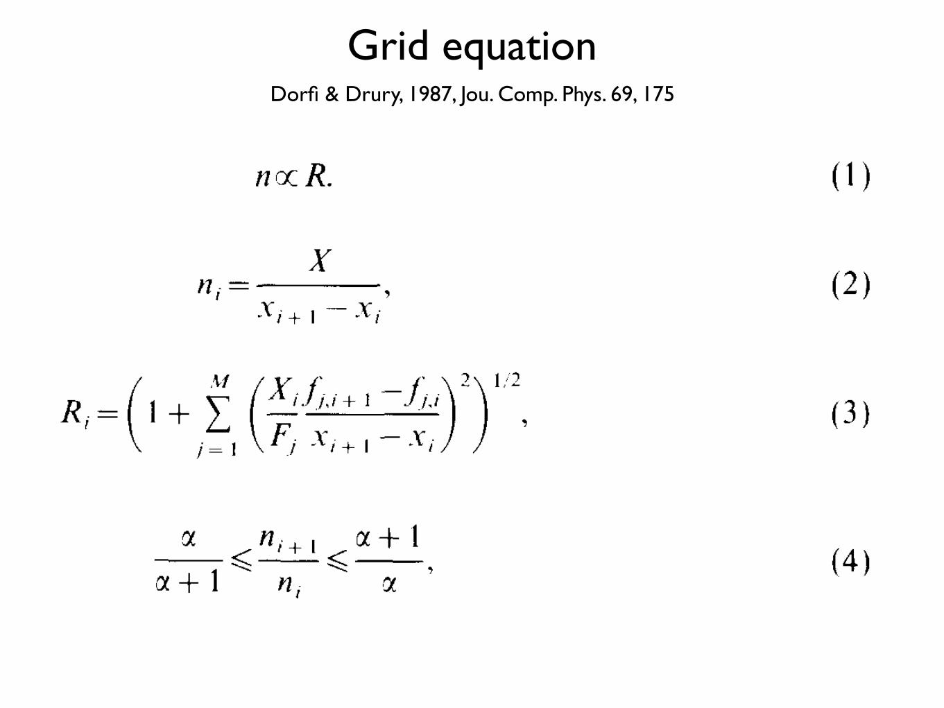
Grid equationDorfi & Drury, 1987, Jou. Comp. Phys. 69, 175

SIMPLE ADAPTIVE GRIDS 177

stant of proportionality being determined by the total number of points and the separation of the bondaries. The fundamental form of our grid equation is thus

nxR. (1)

However, because stability considerations usually require that the point concen- tration not change too rapidly in either space or time, we make n proportional not directly to R, but to the result of applying temporal and spatial smoothing operators to R.

The point concentration we define to be the number of grid points per length scale,

x n, =

.Y 1+1 - x,’

where X is a natural length scale (which may be any smooth positive function of space and time) determined by the problem. In the absence of structure in the solution a default grid is defined by n constant. Thus if X is independent of x the default distribution will be uniform and if X=x it will be logarithmic. More com- plicated default grids can easily be created by choosing appropriate definitions of X.

The desired resolution, R, is a more subjective quantity whose definition necessarily depends on the nature of the problem being solved, the numerical method being used and the personal bias of the investigator. It is obviously essen- tial that R be positive definite, but apart from this it can be any smooth function of the solution and its derivatives. A simple prescription which we have found to give very satisfactory results is motivated by the idea that in the case of one function,,f, the data points should be distributed uniformly in arc-length along the graph ofJ: This suggess R = Jl + (4flcl.u)’ which we generalize to several functions, f’, ,..., ,fiM, and discretize in the form

(3)

where F, is a natural scale associated with the function f, and f,,, =.C(x;). However, note that unlike [IS] we do not transform to an “arc-length” coordinate. For artificial problems where all variables are of order unity one can of course set all scales X,, F, to unity; however in physical applications they are required on dimen- sional grounds alone.

It is perhaps worth noting that R, must be obtained by discretizing some function R. This ensures that the only slight dependence of R, on the grid point distribution comes from the inevitable discretization error. Clearly the required resolution is an intrinsic property of the problem and its solution which should not depend on the actual grid.

Our choice of spatial smoothing is based on the well-known rule of thumb, that

SIMPLE ADAPTIVE GRIDS 177

stant of proportionality being determined by the total number of points and the separation of the bondaries. The fundamental form of our grid equation is thus

nxR. (1)

However, because stability considerations usually require that the point concen- tration not change too rapidly in either space or time, we make n proportional not directly to R, but to the result of applying temporal and spatial smoothing operators to R.

The point concentration we define to be the number of grid points per length scale,

x n, =

.Y 1+1 - x,’

where X is a natural length scale (which may be any smooth positive function of space and time) determined by the problem. In the absence of structure in the solution a default grid is defined by n constant. Thus if X is independent of x the default distribution will be uniform and if X=x it will be logarithmic. More com- plicated default grids can easily be created by choosing appropriate definitions of X.

The desired resolution, R, is a more subjective quantity whose definition necessarily depends on the nature of the problem being solved, the numerical method being used and the personal bias of the investigator. It is obviously essen- tial that R be positive definite, but apart from this it can be any smooth function of the solution and its derivatives. A simple prescription which we have found to give very satisfactory results is motivated by the idea that in the case of one function,,f, the data points should be distributed uniformly in arc-length along the graph ofJ: This suggess R = Jl + (4flcl.u)’ which we generalize to several functions, f’, ,..., ,fiM, and discretize in the form

(3)

where F, is a natural scale associated with the function f, and f,,, =.C(x;). However, note that unlike [IS] we do not transform to an “arc-length” coordinate. For artificial problems where all variables are of order unity one can of course set all scales X,, F, to unity; however in physical applications they are required on dimen- sional grounds alone.

It is perhaps worth noting that R, must be obtained by discretizing some function R. This ensures that the only slight dependence of R, on the grid point distribution comes from the inevitable discretization error. Clearly the required resolution is an intrinsic property of the problem and its solution which should not depend on the actual grid.

Our choice of spatial smoothing is based on the well-known rule of thumb, that

SIMPLE ADAPTIVE GRIDS 177

stant of proportionality being determined by the total number of points and the separation of the bondaries. The fundamental form of our grid equation is thus

nxR. (1)

However, because stability considerations usually require that the point concen- tration not change too rapidly in either space or time, we make n proportional not directly to R, but to the result of applying temporal and spatial smoothing operators to R.

The point concentration we define to be the number of grid points per length scale,

x n, =

.Y 1+1 - x,’

where X is a natural length scale (which may be any smooth positive function of space and time) determined by the problem. In the absence of structure in the solution a default grid is defined by n constant. Thus if X is independent of x the default distribution will be uniform and if X=x it will be logarithmic. More com- plicated default grids can easily be created by choosing appropriate definitions of X.

The desired resolution, R, is a more subjective quantity whose definition necessarily depends on the nature of the problem being solved, the numerical method being used and the personal bias of the investigator. It is obviously essen- tial that R be positive definite, but apart from this it can be any smooth function of the solution and its derivatives. A simple prescription which we have found to give very satisfactory results is motivated by the idea that in the case of one function,,f, the data points should be distributed uniformly in arc-length along the graph ofJ: This suggess R = Jl + (4flcl.u)’ which we generalize to several functions, f’, ,..., ,fiM, and discretize in the form

(3)

where F, is a natural scale associated with the function f, and f,,, =.C(x;). However, note that unlike [IS] we do not transform to an “arc-length” coordinate. For artificial problems where all variables are of order unity one can of course set all scales X,, F, to unity; however in physical applications they are required on dimen- sional grounds alone.

It is perhaps worth noting that R, must be obtained by discretizing some function R. This ensures that the only slight dependence of R, on the grid point distribution comes from the inevitable discretization error. Clearly the required resolution is an intrinsic property of the problem and its solution which should not depend on the actual grid.

Our choice of spatial smoothing is based on the well-known rule of thumb, that

178 DORFI AND DRURY

for stability the grid spacing should not change from one interval to the next by more than about 20 or 30%. We interpret this as the requirement

a n !+I cc+ 1 d----d- a+1 n, x ’ (4)

where c( is a measure of the grid “rigidity.” The simplest way to achieve this, bearing in mind that R is positive definite. is to smooth the right-hand side of Eq. (1) and write

(5)

but this smoothing kernel (neglecting for the moment the question of the boundary conditions) is the Green’s function associated with the difference operator

1 -r(a + 1) 6’, (6)

where 6 denotes a centred difference. Thus we can replace the smoothing on the right by a differencing on the left and write

fi,=n,-x(a+l)(n,+,-2n,+n, ,)xR,. (7)

Actually as boundary conditions for the grid equation we set the concentration gradient to zero,

n, =n7, n ,% ?=nv , (8)

so that the true Green’s function is slightly more complicated, but the difference is imperceptible except near a boundary.

To smooth the time dependence we use a similar idea, in effect replacing R(t) by

R( t - f’ ) exp( - t/s) dt’/r. (9)

To achieve this we write equation in the form

ri;=ii,+~(ii,-ri:“‘“~)rR,, (10)

where At is the time step. The grid then adjusts on a time-scale z and ignores variations on shorter time-scales. As with the other scales, 7 can be a constant, or vary in some smooth fashion appropriate to the problem.

Finally we eliminate the constant of proportionality and obtain the grid equation,

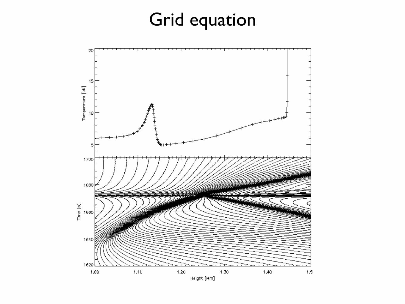
Grid equation

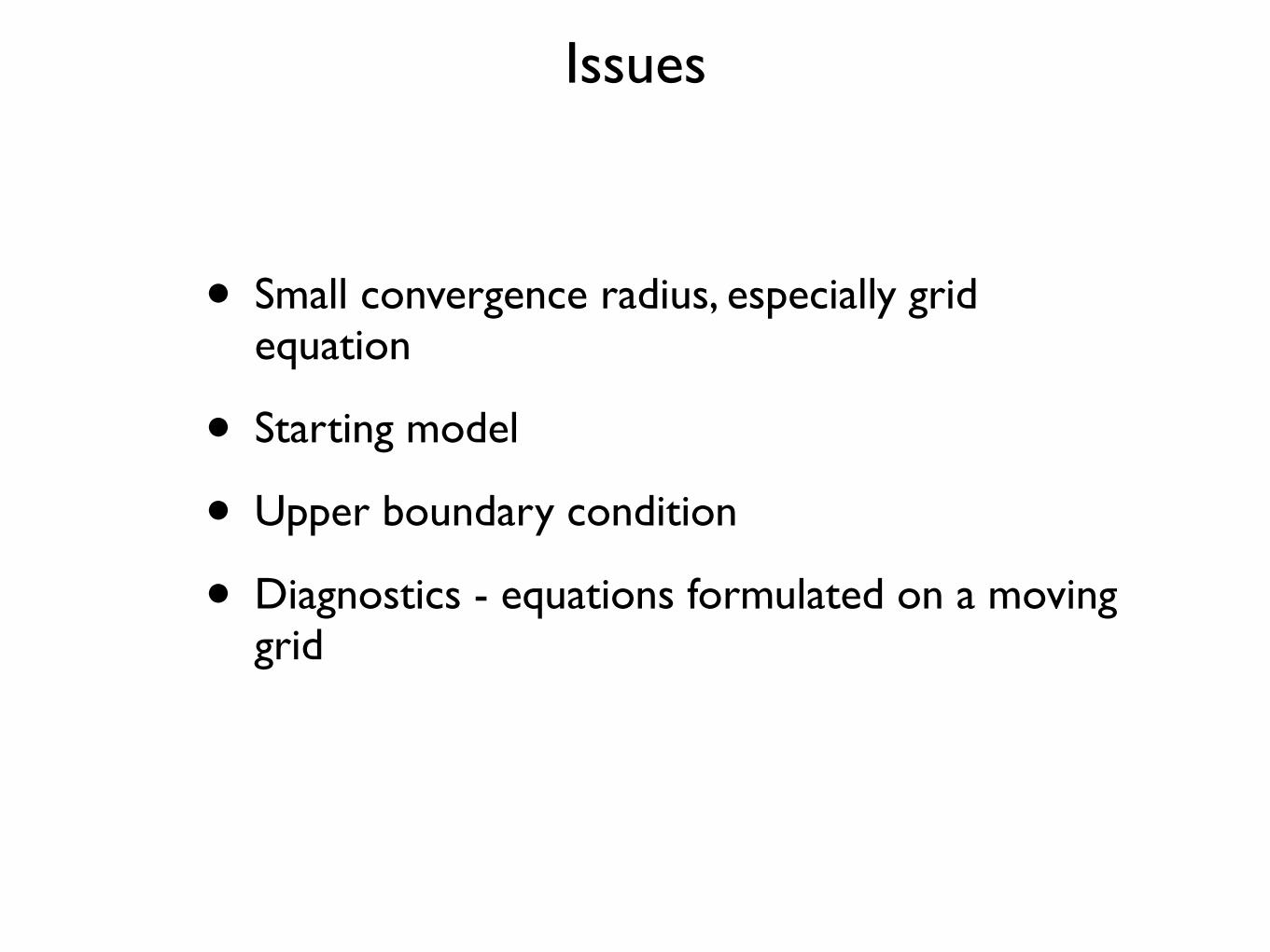
Issues

• Small convergence radius, especially grid equation

• Starting model

• Upper boundary condition

• Diagnostics - equations formulated on a moving grid

Small convergence radius

• Careful control of timestep

• Use relaxation instead of static equations

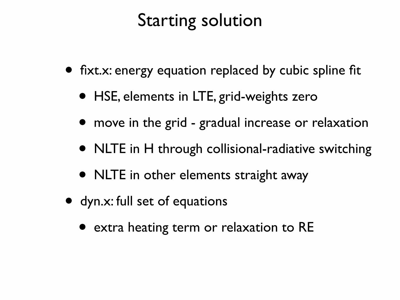
Starting solution

• fixt.x: energy equation replaced by cubic spline fit

• HSE, elements in LTE, grid-weights zero

• move in the grid - gradual increase or relaxation

• NLTE in H through collisional-radiative switching

• NLTE in other elements straight away

• dyn.x: full set of equations

• extra heating term or relaxation to RE

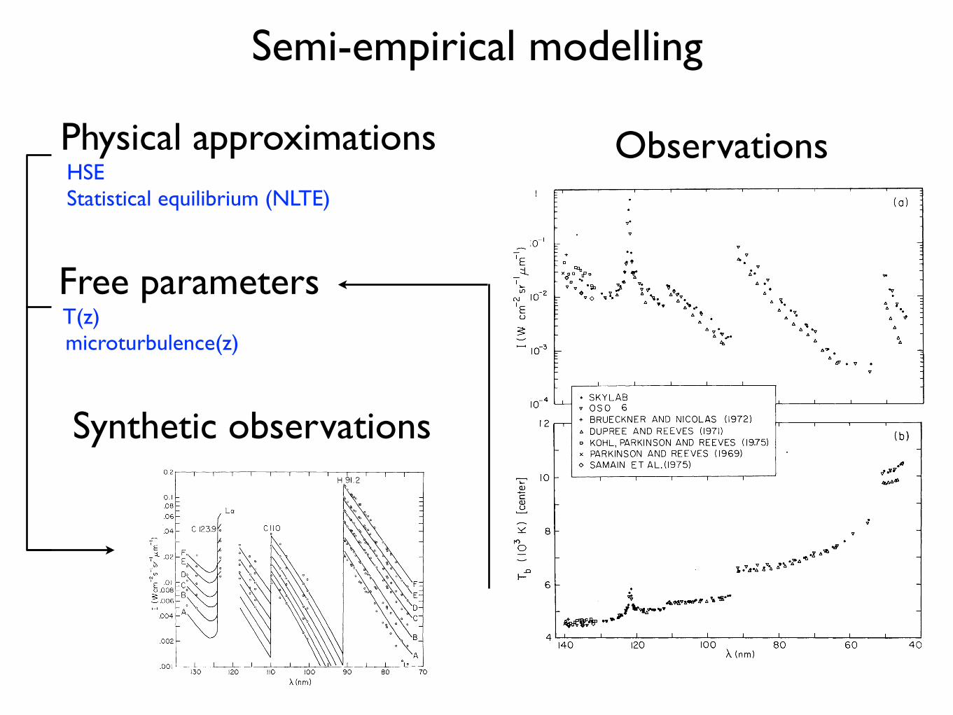
Semi-empirical modelling

ObservationsPhysical approximations HSE Statistical equilibrium (NLTE)

Free parameters T(z) microturbulence(z)

Synthetic observations1981ApJS...45..635V

1981ApJS...45..635V

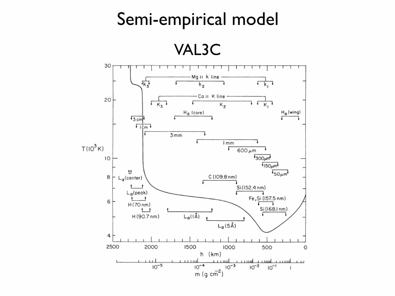
Semi-empirical model

VAL3C

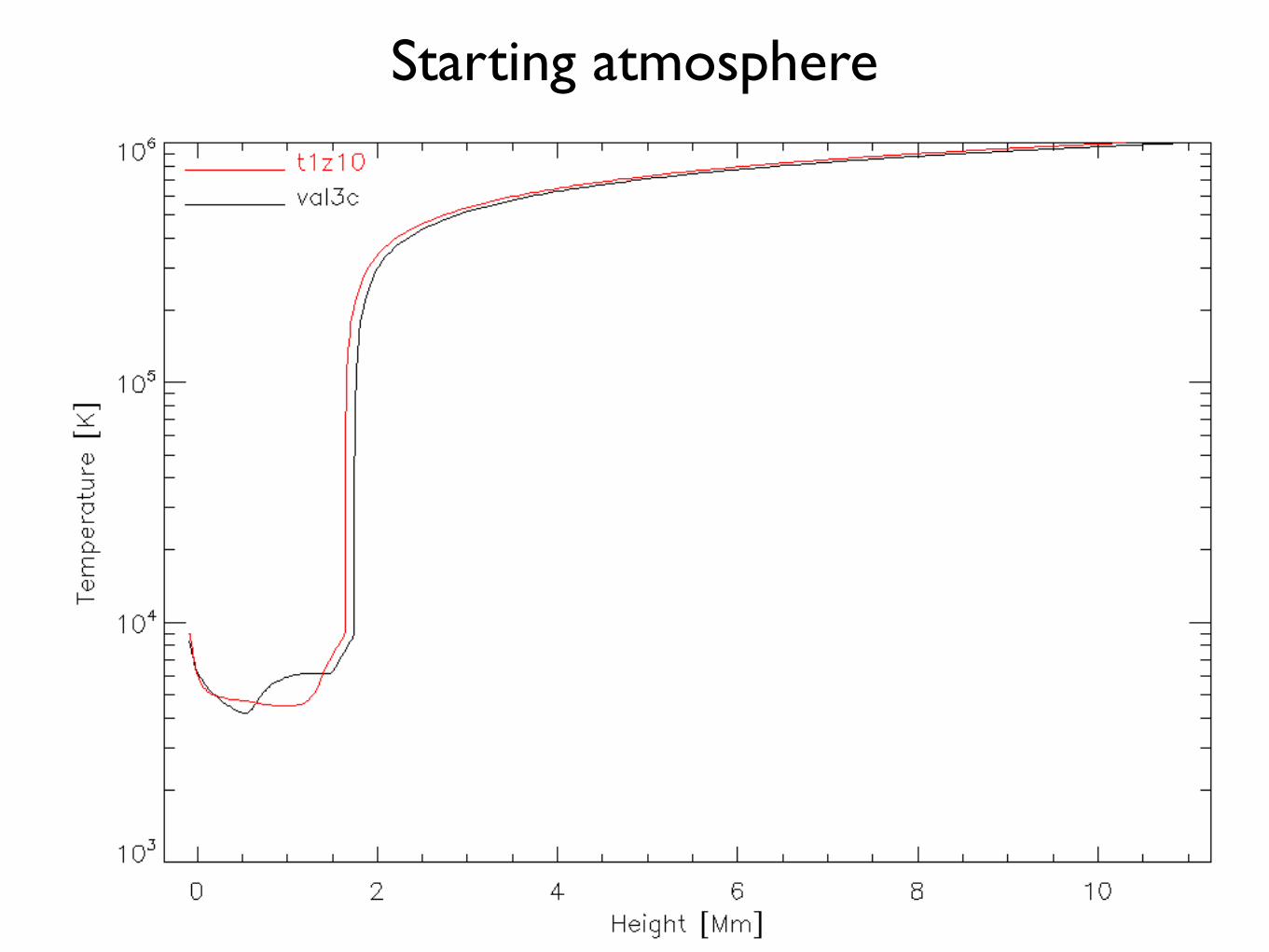
Starting atmosphere

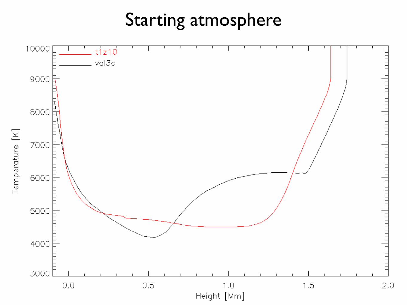
Starting atmosphere

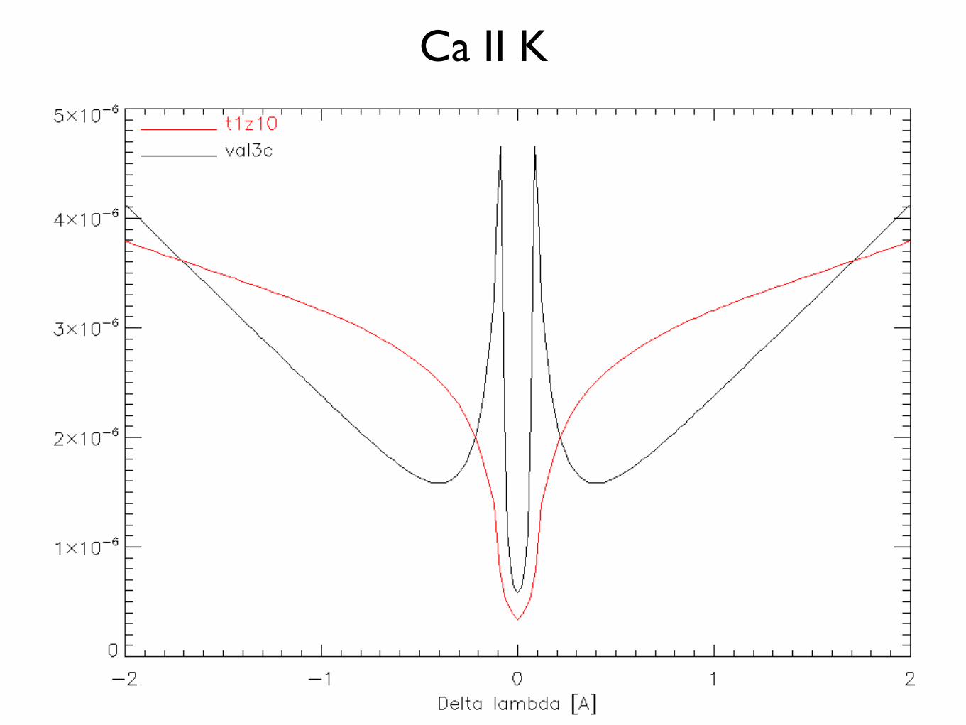
Ca II K

Upper boundary condition

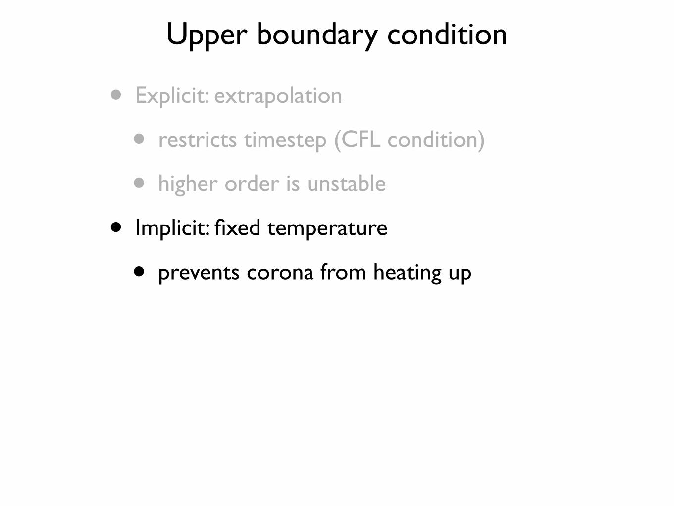
• Explicit: extrapolation

• restricts timestep (CFL condition)

• higher order is unstable

Upper boundary condition

• Explicit: extrapolation

• restricts timestep (CFL condition)

• higher order is unstable

• Implicit: fixed temperature

• prevents corona from heating up

Upper boundary condition

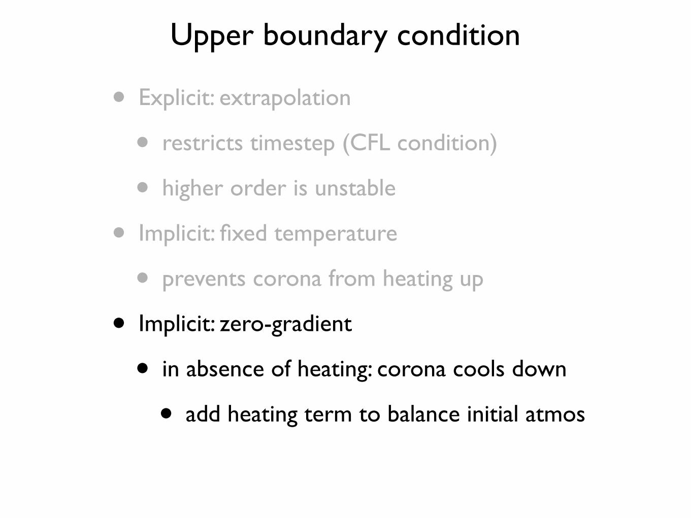
• Explicit: extrapolation

• restricts timestep (CFL condition)

• higher order is unstable

• Implicit: fixed temperature

• prevents corona from heating up

• Implicit: zero-gradient

• in absence of heating: corona cools down

• add heating term to balance initial atmos

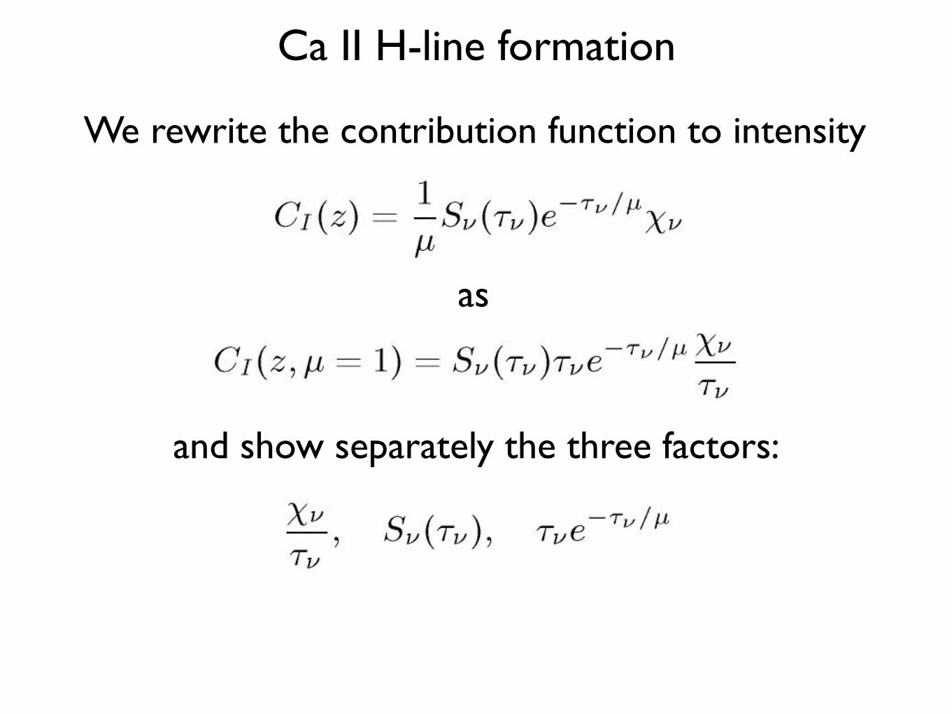
Ca II H-line formation

We rewrite the contribution function to intensity

as

and show separately the three factors:

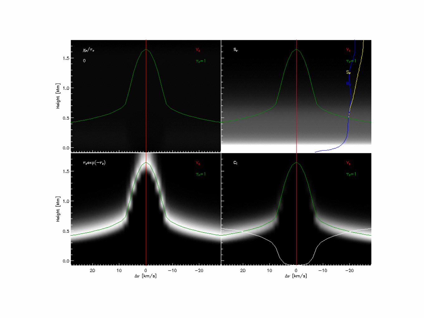
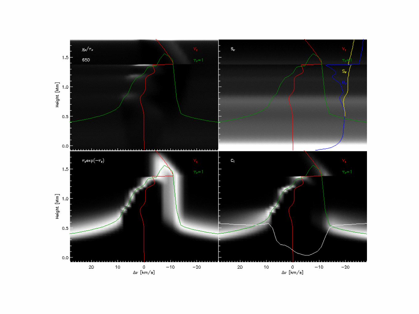
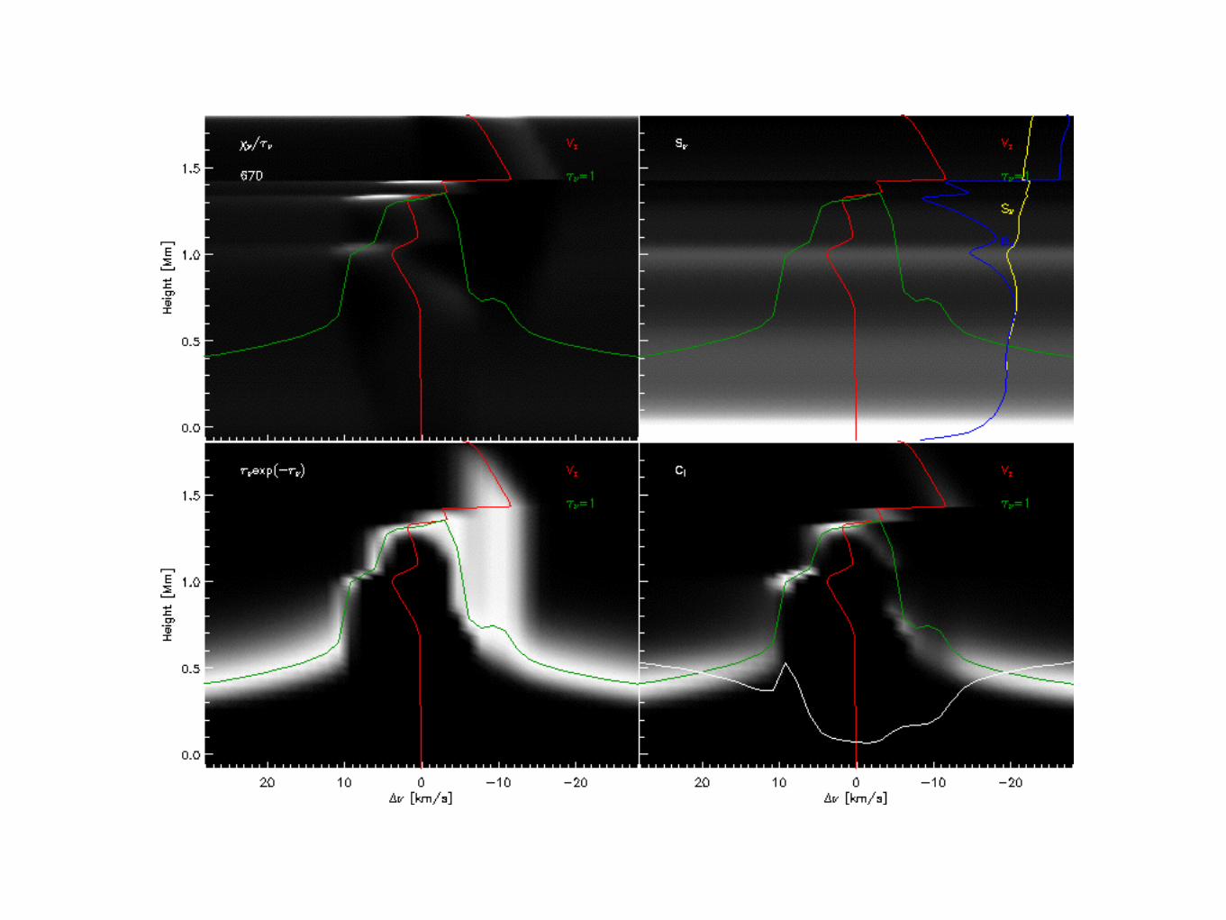
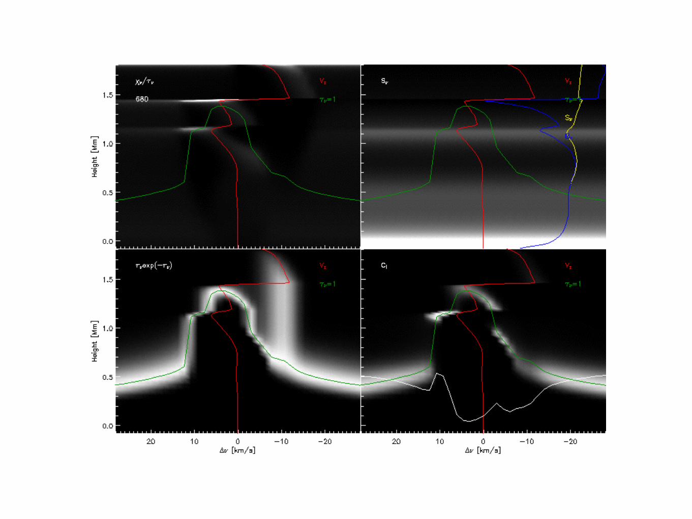
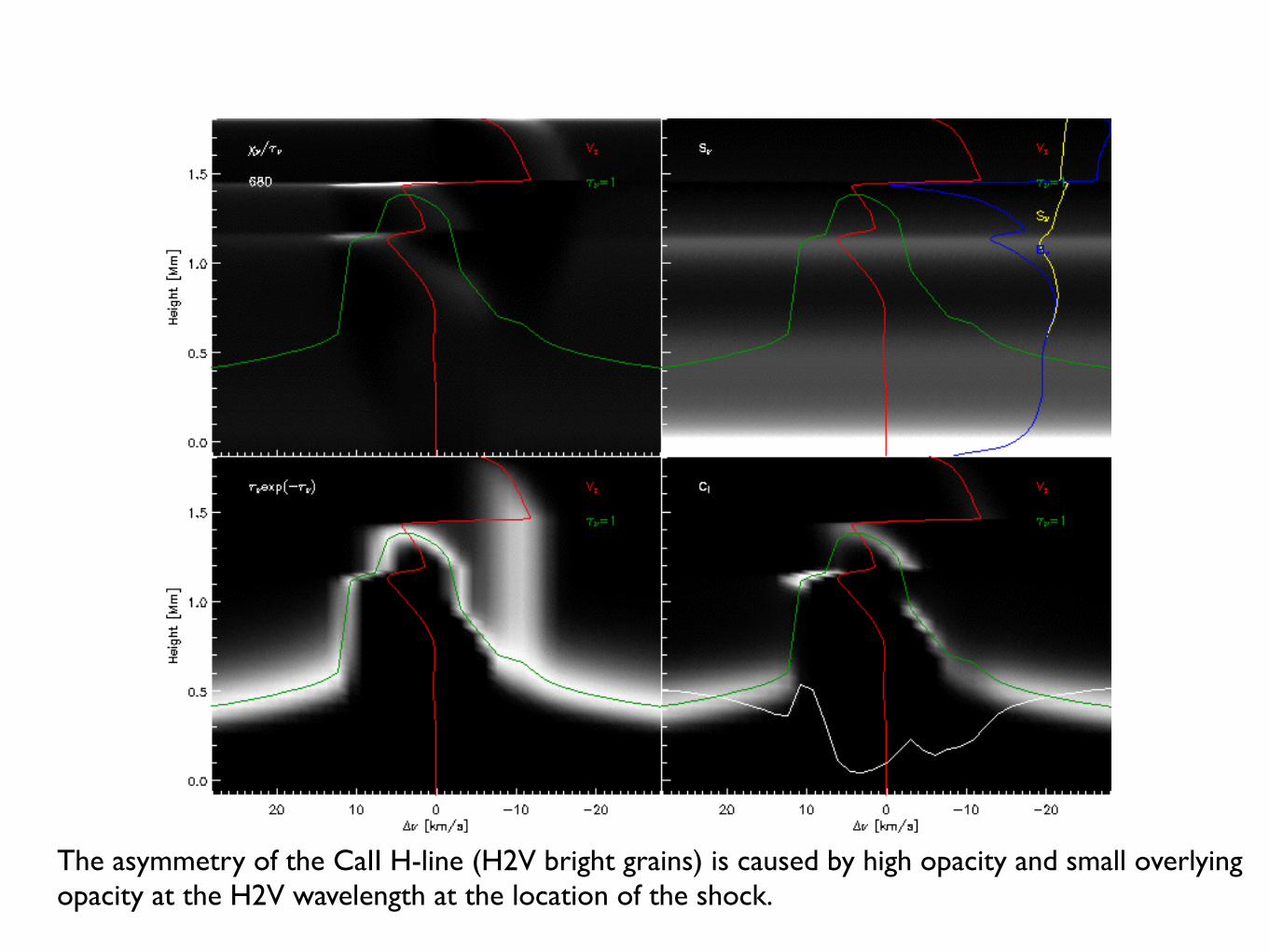
The asymmetry of the CaII H-line (H2V bright grains) is caused by high opacity and small overlying opacity at the H2V wavelength at the location of the shock.

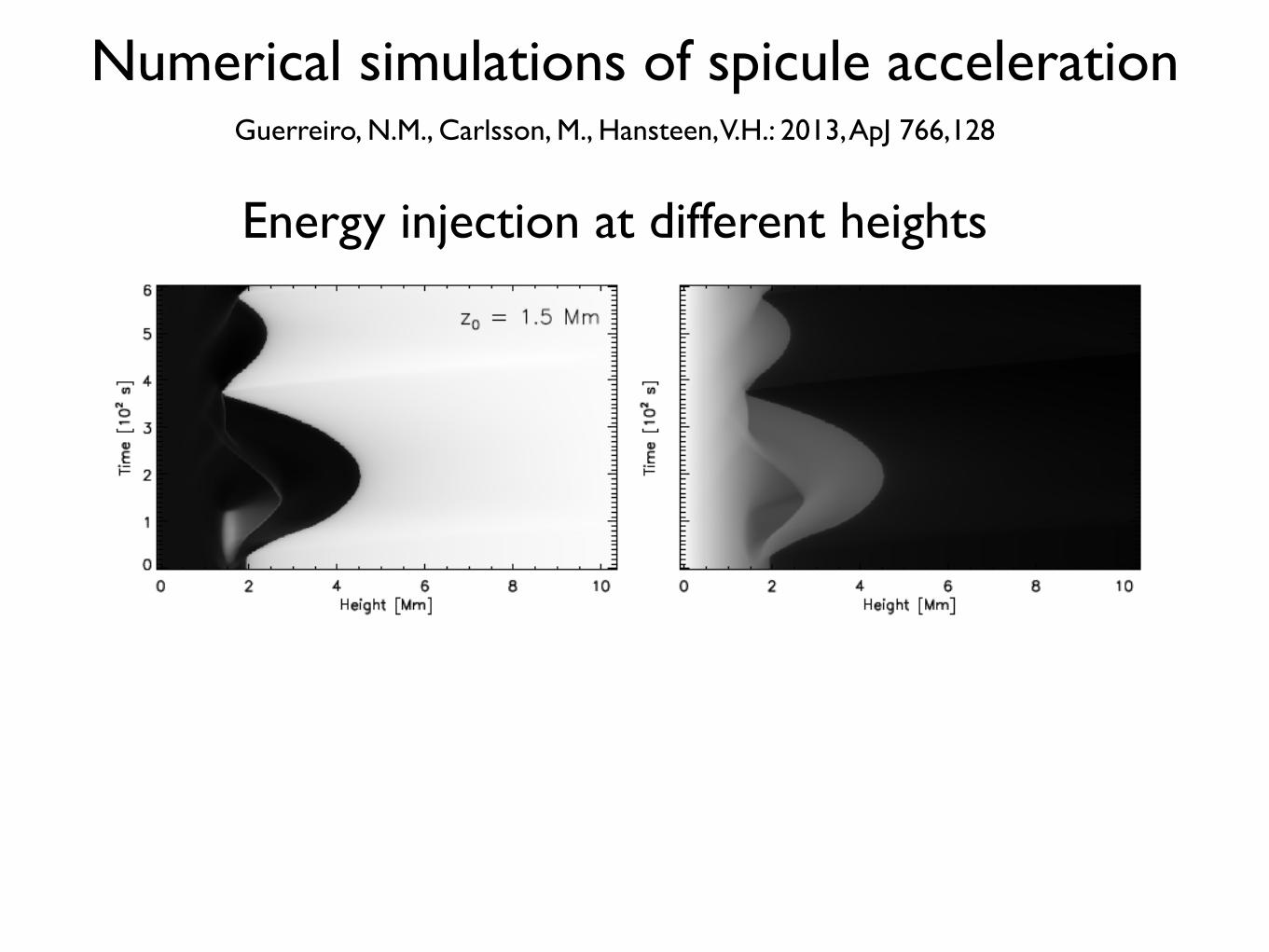
Numerical simulations of spicule accelerationGuerreiro, N.M., Carlsson, M., Hansteen, V.H.: 2013, ApJ 766,128

Energy injection at different heights

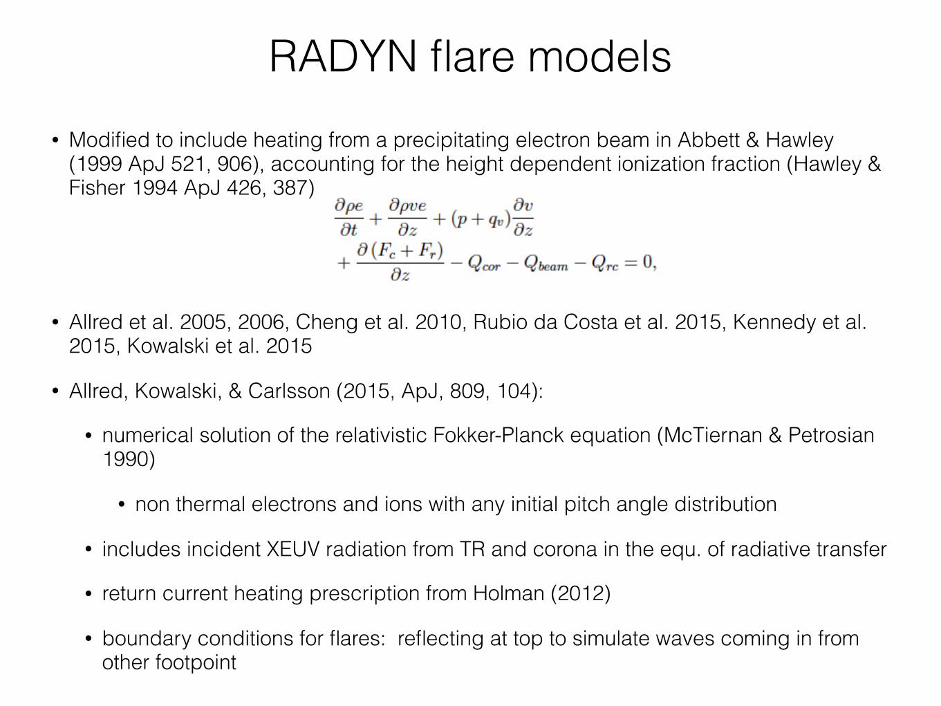
RADYN flare models • Modified to include heating from a precipitating electron beam in Abbett & Hawley

(1999 ApJ 521, 906), accounting for the height dependent ionization fraction (Hawley & Fisher 1994 ApJ 426, 387)

• Allred et al. 2005, 2006, Cheng et al. 2010, Rubio da Costa et al. 2015, Kennedy et al. 2015, Kowalski et al. 2015

• Allred, Kowalski, & Carlsson (2015, ApJ, 809, 104):

• numerical solution of the relativistic Fokker-Planck equation (McTiernan & Petrosian 1990)

• non thermal electrons and ions with any initial pitch angle distribution

• includes incident XEUV radiation from TR and corona in the equ. of radiative transfer

• return current heating prescription from Holman (2012)

• boundary conditions for flares: reflecting at top to simulate waves coming in from other footpoint

RADYN flare models

• Studying chromospheric evaporation and condensation phenomena.

• Predictions for optically thick line and continuum diagnostics from a complicated, evolving atmosphere with many sources of opacities. Self-consistently models an atmosphere with height dependent ionization fraction, temperature, velocity field, atomic rates not in equilibrium.

• 1D, plane-parallel: simulating the center of a flux tube, motion confined to one dimension.

• Can use the atmospheric properties at each time-step to obtain predictions for optically thin emission, given the assumptions used in CHIANTI.

• IRIS diagnostics that are optically thin: Si IV, O IV, Fe XII, Fe XXI.

Tutorial material• unpack radyn_tutorial.tar

• creates directory radyn_tutorial

• go to directory radyn_tutorial

• analysis_tools.pdf contains manual for tools

• IDL routines

• sample RADYN output

• more RADYN output in

• http://folk.uio.no/matsc/radyn/grid

Outline of tutorial

• Introduce you to the input file, ftab.dat

• IDL output files: have you read in with IDL

• mxmovie.pro : to visualize time evolution

• emovie.pro: to visualize energy terms

• rad_thinline_intensity.pro : to produce light curve and contribution function of Si IV, O IV, Fe XXI

• use contribution function to investigate atmospheric properties where emission is produced

• radxdetailed.pro: H alpha, He II 304, continuum

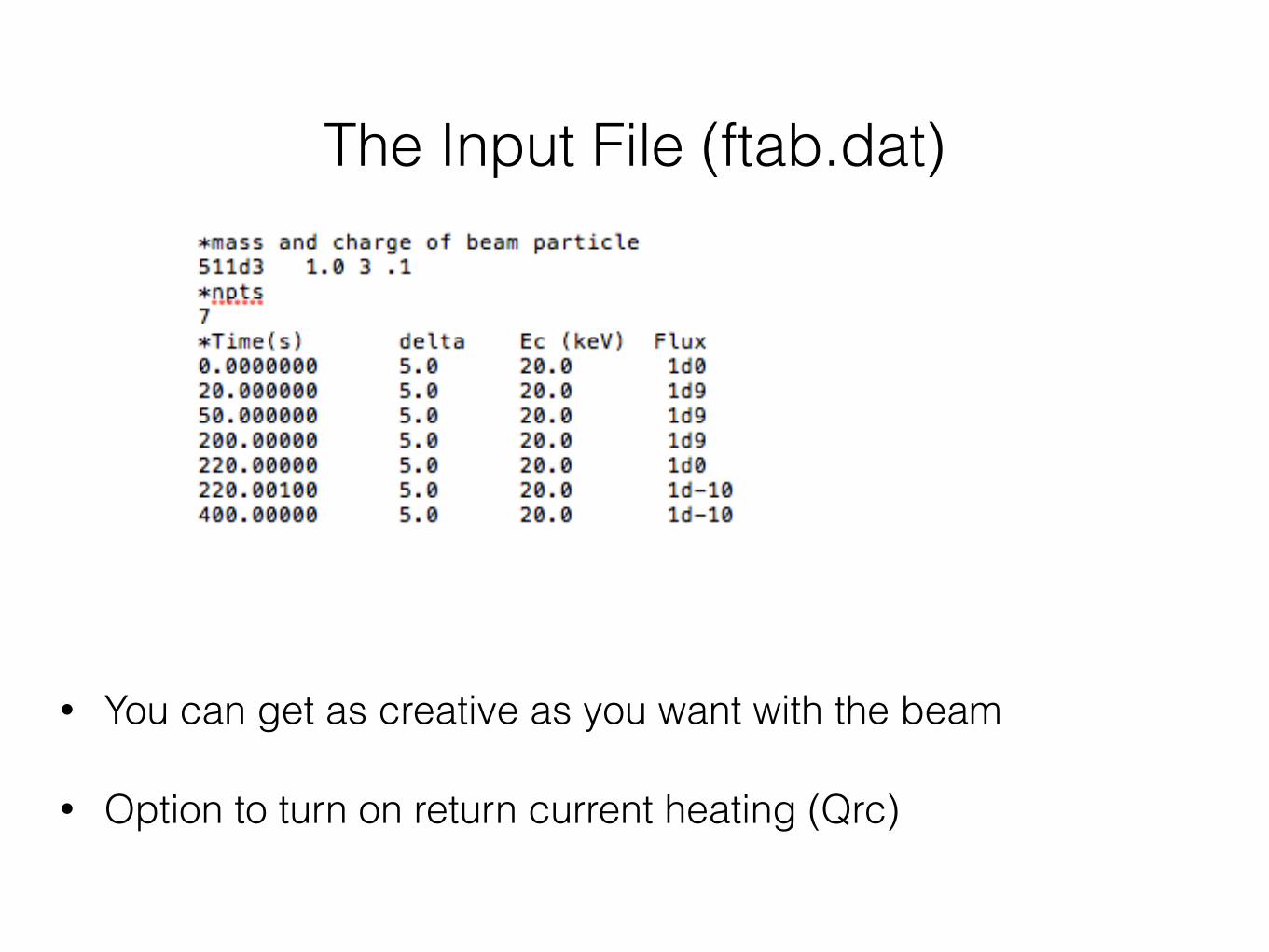
The Input File (ftab.dat)

• You can get as creative as you want with the beam

• Option to turn on return current heating (Qrc)

511d3 = mass of particle in eV (electron or proton)1.0 = absolute value of charge of particle3 = Gaussian distribution of pitch angles in forward hemisphere ( =2 -> isotropic in forward hemisphere) 0.1 = pitch angle sigma for Gaussian

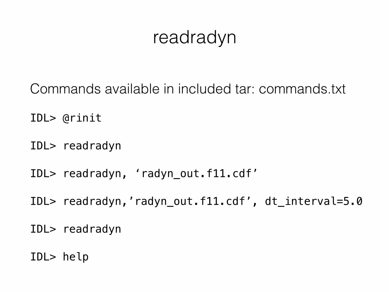
Commands available in included tar: commands.txt

IDL> @rinit

IDL> readradyn

IDL> readradyn, ‘radyn_out.f11.cdf’

IDL> readradyn,’radyn_out.f11.cdf’, dt_interval=5.0

IDL> readradyn

IDL> help

readradyn

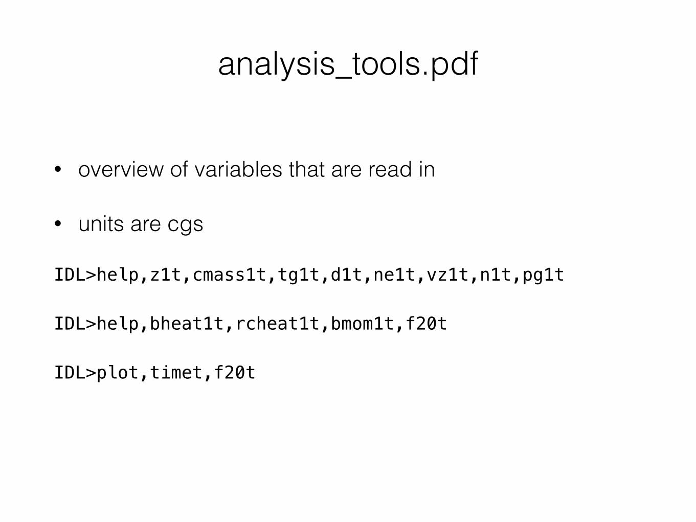
analysis_tools.pdf

• overview of variables that are read in

• units are cgs

IDL>help,z1t,cmass1t,tg1t,d1t,ne1t,vz1t,n1t,pg1t

IDL>help,bheat1t,rcheat1t,bmom1t,f20t

IDL>plot,timet,f20t

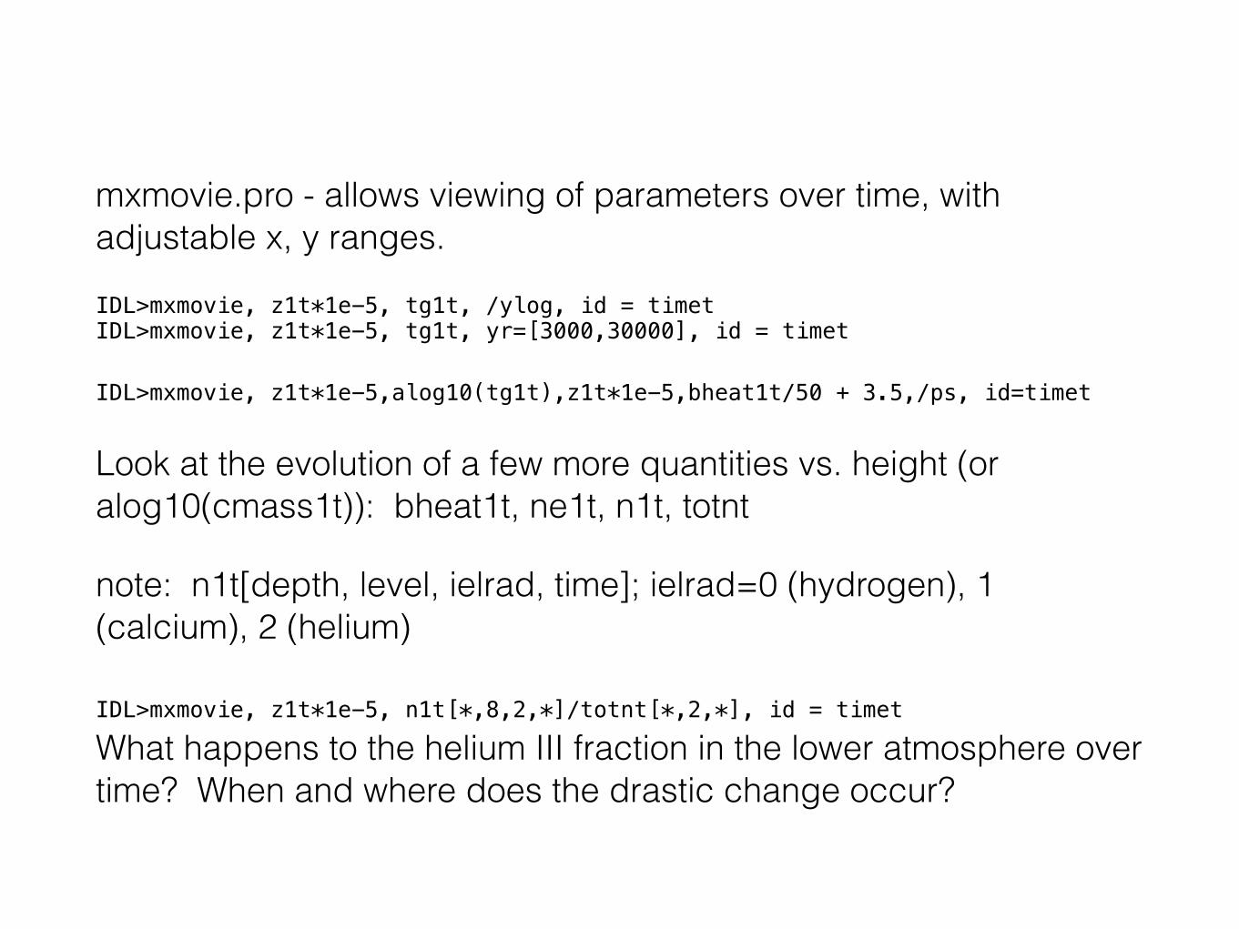
mxmovie.pro - allows viewing of parameters over time, with adjustable x, y ranges.

IDL>mxmovie, z1t*1e-5, tg1t, /ylog, id = timet IDL>mxmovie, z1t*1e-5, tg1t, yr=[3000,30000], id = timet

IDL>mxmovie, z1t*1e-5,alog10(tg1t),z1t*1e-5,bheat1t/50 + 3.5,/ps, id=timet

Look at the evolution of a few more quantities vs. height (or alog10(cmass1t)): bheat1t, ne1t, n1t, totnt

note: n1t[depth, level, ielrad, time]; ielrad=0 (hydrogen), 1 (calcium), 2 (helium)

IDL>mxmovie, z1t*1e-5, n1t[*,8,2,*]/totnt[*,2,*], id = timet What happens to the helium III fraction in the lower atmosphere over time? When and where does the drastic change occur?

rmovie.pro

Problems with XQuartz 2.7.10 on Mac

Error: attempt to add non-widget child "dsm" to parent "idl" which supports only widgets

Solution:sudo mv /opt/X11/lib/libXt.6.dylib{,.bak}sudo cp /opt/X11/lib{/flat_namespace,}/libXt.6.dylib

rad2plot.pro: analyzing gentle evaporationIDL> rad2plot

• plotting two variables vs. height (or column mass) in same window at a given time

• Now try:

IDL> rad2plot, z1t*1e-5, alog10(tg1t), bheat1t, 20

• Zoom in on the location of maximum beam energy deposition.

• Note: bheat1t/d1t is also useful to consider

• Examine the beam energy deposition at t=50 s, over plotting the pre flare quantities:

IDL>rad2plot, z1t*1e-5, alog10(tg1t), bheat1t, 50, /oplot_t0

rad2plot.pro: analyzing gentle evaporation

• Examine the gas pressure and velocity at t=15s (pre-flare atmosphere will be over plotted):

IDL> rad2plot, z1t*1e-5, alog10(pg1t), vz1t*1e-5, 15, /oplot_t0, xr = [0,2000], yr = [0,5], y2r = [-2,3]

• What is the reason for the upward and downward directed velocities at this time?

IDL> rad2plot, z1t*1e-5, alog10(pg1t), alog10(tg1t), 15, /oplot_t0,xr = [0,2000], yr = [0,5], y2r = [3.5,4.5]

IDL> rad2plot, z1t*1e-5, alog10(tg1t), vz1t*1e-5, 20, /oplot_t0, xr=[0, 2000], yr=[3.5, 5], y2r=[-10, 10]

• Why does the transition region appear at a higher height at t=20s compared to t=0s?

rad2plot.pro: analyzing gentle evaporation

• Now use mxmovie to follow the velocity evolution

IDL> mxmovie, z1t*1e-5, vz1t*1e-5

• Other useful quantities: e.g., ionization fraction:

IDL> rad2plot, z1t*1e-5, alog10(tg1t), n1t[*,5,0,*]/totnt[*,0,*], 20., xr = [0,2000]

IDL> rad2plot, z1t*1e-5, alog10(tg1t), n1t[*,8,2,*]/totnt[*,2,*], 75., xr = [0,3000], y2r = [0,1]

Why does the helium III fraction change, as you found earlier?

rad_thinline_intensity.pro

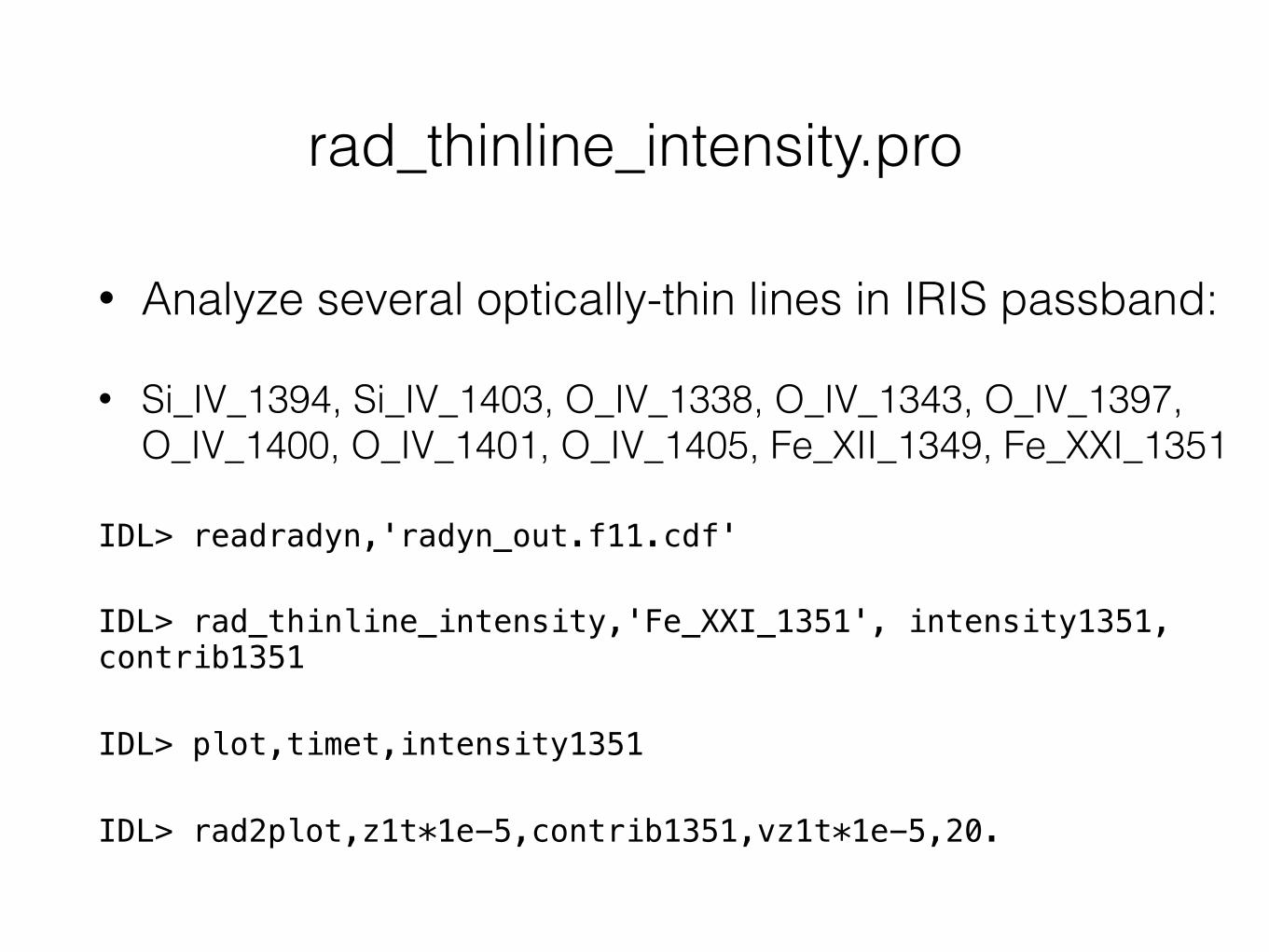
• Analyze several optically-thin lines in IRIS passband:

• Si_IV_1394, Si_IV_1403, O_IV_1338, O_IV_1343, O_IV_1397, O_IV_1400, O_IV_1401, O_IV_1405, Fe_XII_1349, Fe_XXI_1351

IDL> readradyn,'radyn_out.f11.cdf'

IDL> rad_thinline_intensity,'Fe_XXI_1351', intensity1351, contrib1351

IDL> plot,timet,intensity1351

IDL> rad2plot,z1t*1e-5,contrib1351,vz1t*1e-5,20.

rad_thinline_intensity.pro

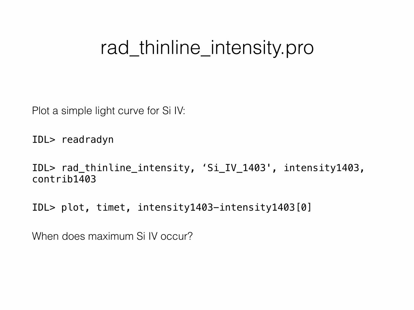
Plot a simple light curve for Si IV:

IDL> readradyn

IDL> rad_thinline_intensity, ‘Si_IV_1403', intensity1403, contrib1403

IDL> plot, timet, intensity1403-intensity1403[0]

When does maximum Si IV occur?

rad_thinline_intensity.pro

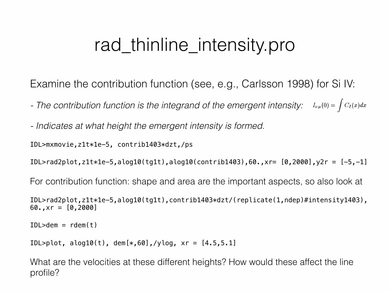
Examine the contribution function (see, e.g., Carlsson 1998) for Si IV:

- The contribution function is the integrand of the emergent intensity:

- Indicates at what height the emergent intensity is formed.

IDL>mxmovie,z1t*1e-5, contrib1403*dzt,/ps

IDL>rad2plot,z1t*1e-5,alog10(tg1t),alog10(contrib1403),60.,xr= [0,2000],y2r = [-5,-1]

For contribution function: shape and area are the important aspects, so also look at

IDL>rad2plot,z1t*1e-5,alog10(tg1t),contrib1403*dzt/(replicate(1,ndep)#intensity1403),60.,xr = [0,2000]

IDL>dem = rdem(t)

IDL>plot, alog10(t), dem[*,60],/ylog, xr = [4.5,5.1]

What are the velocities at these different heights? How would these affect the line profile?

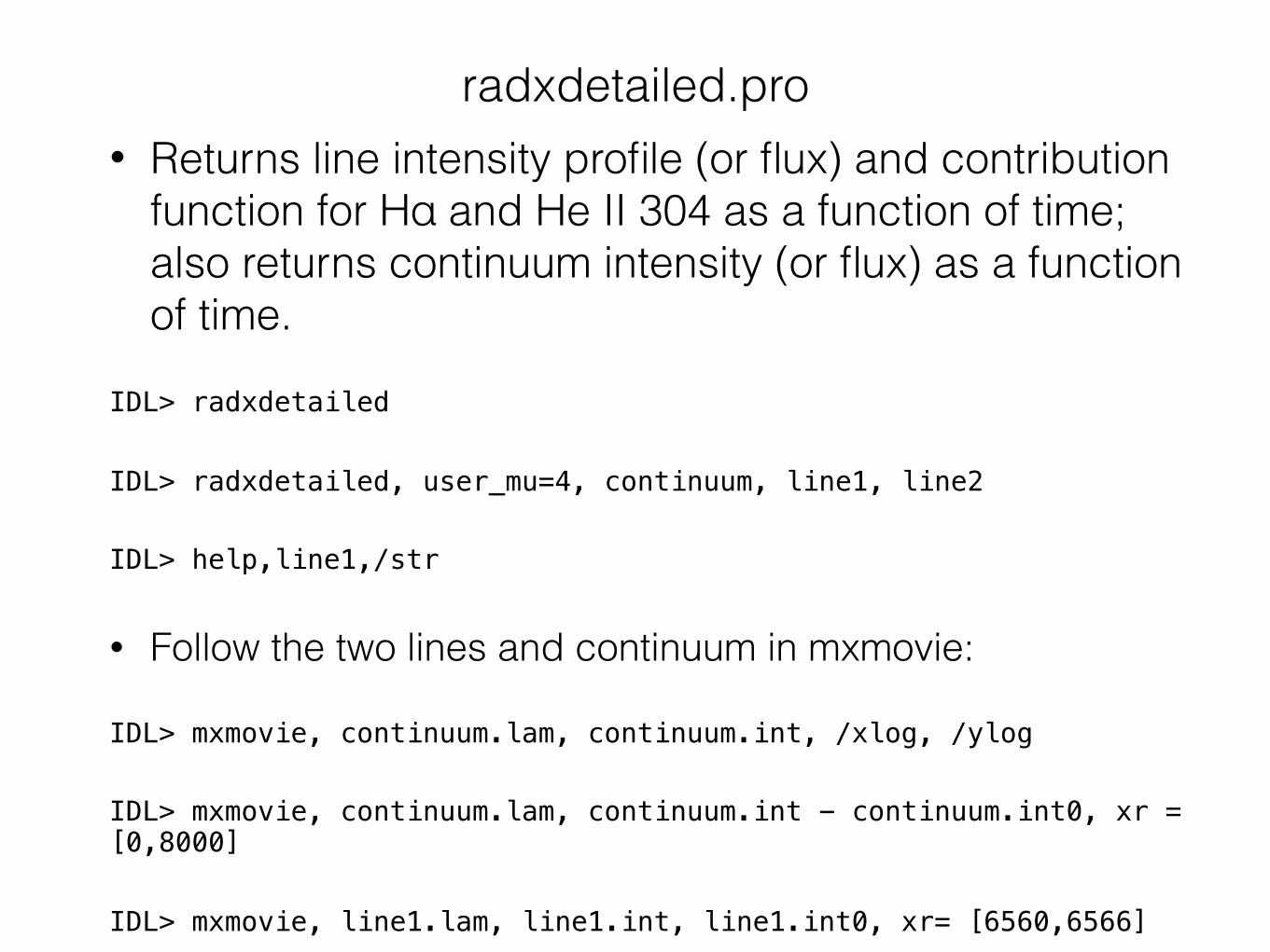
• Returns line intensity profile (or flux) and contribution function for Hα and He II 304 as a function of time; also returns continuum intensity (or flux) as a function of time.

IDL> radxdetailed

IDL> radxdetailed, user_mu=4, continuum, line1, line2

IDL> help,line1,/str

• Follow the two lines and continuum in mxmovie:

IDL> mxmovie, continuum.lam, continuum.int, /xlog, /ylog

IDL> mxmovie, continuum.lam, continuum.int - continuum.int0, xr = [0,8000]

IDL> mxmovie, line1.lam, line1.int, line1.int0, xr= [6560,6566]

radxdetailed.pro

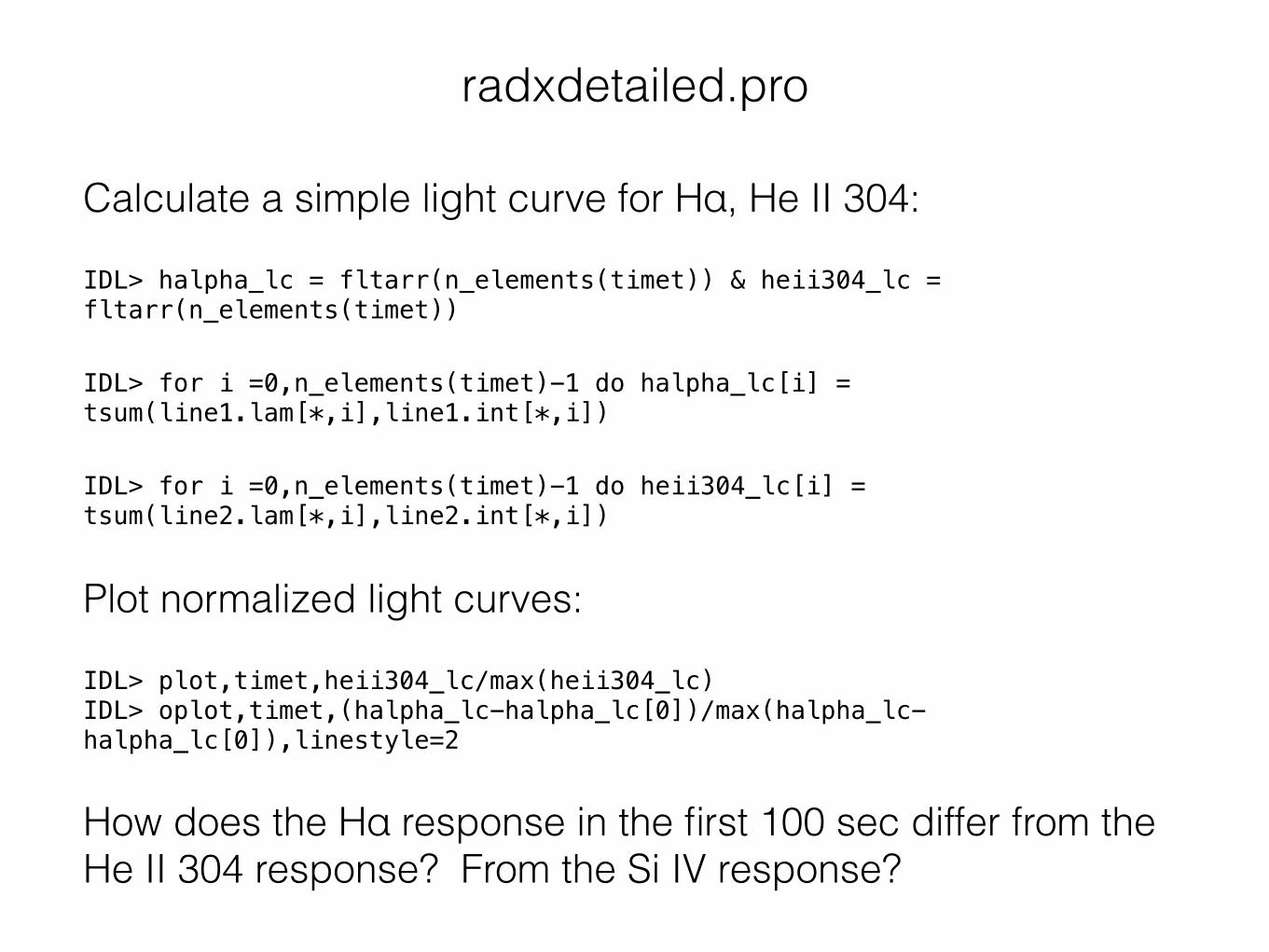
Calculate a simple light curve for Hα, He II 304:

IDL> halpha_lc = fltarr(n_elements(timet)) & heii304_lc = fltarr(n_elements(timet))

IDL> for i =0,n_elements(timet)-1 do halpha_lc[i] = tsum(line1.lam[*,i],line1.int[*,i])

IDL> for i =0,n_elements(timet)-1 do heii304_lc[i] = tsum(line2.lam[*,i],line2.int[*,i])

Plot normalized light curves:

IDL> plot,timet,heii304_lc/max(heii304_lc) IDL> oplot,timet,(halpha_lc-halpha_lc[0])/max(halpha_lc-halpha_lc[0]),linestyle=2

How does the Hα response in the first 100 sec differ from the He II 304 response? From the Si IV response?

radxdetailed.pro

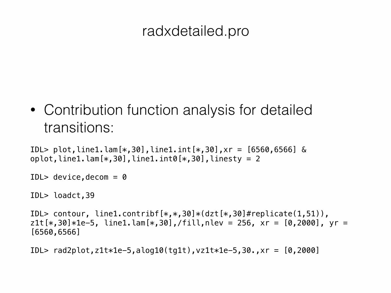
• Contribution function analysis for detailed transitions:

IDL> plot,line1.lam[*,30],line1.int[*,30],xr = [6560,6566] & oplot,line1.lam[*,30],line1.int0[*,30],linesty = 2

IDL> device,decom = 0

IDL> loadct,39

IDL> contour, line1.contribf[*,*,30]*(dzt[*,30]#replicate(1,51)), z1t[*,30]*1e-5, line1.lam[*,30],/fill,nlev = 256, xr = [0,2000], yr = [6560,6566]

IDL> rad2plot,z1t*1e-5,alog10(tg1t),vz1t*1e-5,30.,xr = [0,2000]

radxdetailed.pro

• There are more detailed transitions available to analyze (see Allred et al. 2015).

• The IRIS lines Mg II and C II are not calculated directly in these models we’ve given you. Including other elements/transitions in RADYN is not trivial and is ongoing work.

• One can take RADYN snapshots and put them through the RH code (Uitenbroek 2001), which is now publicly available for download from the IRIS website.

Other detailed transitions?