15 The Renormalization Group
37
15 The Renormalization Group 15.1 Scale dependence in Quantum Field Theory and in Statistical Physics In earlier chapters we used perturbation theory to compute the N -point functions in field theory, focusing on φ 4 theory. There we used a time- honored approach which has been successful in theories such as quantum electrodynamics. Already at low orders in this expansion we found difficul- ties in the form of divergent contributions at every order. In comparison with Quantum Mechanics, this problems may seem unusual and troubling. In Quantum Mechanics, Rayleigh-Schr¨ odinger perturbation theory is finite term by term in the expansion, even though the resulting series may not be convergent, e.g. an expansion in powers of the coupling constant of the non- linear term in an anharmonic oscillator. Instead, in Quantum Field Theory, one generally has divergent contributions at every order in perturbation the- ory. In order to handle these divergent contributions one introduces a set of effective (or renormalized) quantities. In this approach, the singular behav- ior is hidden in the relation between bare and renormalized quantities. This approach looks like one is sweeping the problem under a rug and, in fact, it is so. Quite early on (in 1954), Murray Gell-Mann and Francis Low (Gell-Mann and Low, 1954) proposed to take a somewhat different look at the renormal- ization process in Quantum Field Theory (QED in their case), by recasting the renormalization of the coupling constant as the solution of a differen- tial equation. The renormalization process tells us that we can change the bare coupling λ and the UV cutoffΛ while, at the same time, keeping the renormalized coupling constant fixed at some value g. This process defines
Transcript of 15 The Renormalization Group
15
The Renormalization Group
15.1 Scale dependence in Quantum Field Theory and in
Statistical Physics
In earlier chapters we used perturbation theory to compute the N -pointfunctions in field theory, focusing on φ
4 theory. There we used a time-honored approach which has been successful in theories such as quantumelectrodynamics. Already at low orders in this expansion we found difficul-ties in the form of divergent contributions at every order. In comparisonwith Quantum Mechanics, this problems may seem unusual and troubling.In Quantum Mechanics, Rayleigh-Schrodinger perturbation theory is finiteterm by term in the expansion, even though the resulting series may not beconvergent, e.g. an expansion in powers of the coupling constant of the non-linear term in an anharmonic oscillator. Instead, in Quantum Field Theory,one generally has divergent contributions at every order in perturbation the-ory. In order to handle these divergent contributions one introduces a set ofeffective (or renormalized) quantities. In this approach, the singular behav-ior is hidden in the relation between bare and renormalized quantities. Thisapproach looks like one is sweeping the problem under a rug and, in fact, itis so.
Quite early on (in 1954), Murray Gell-Mann and Francis Low (Gell-Mannand Low, 1954) proposed to take a somewhat different look at the renormal-ization process in Quantum Field Theory (QED in their case), by recastingthe renormalization of the coupling constant as the solution of a differen-tial equation. The renormalization process tells us that we can change thebare coupling λ and the UV cutoff Λ while, at the same time, keeping therenormalized coupling constant fixed at some value g. This process defines
494 The Renormalization Group
a function, the Gell-Mann-Low beta-function β(λ), defined by
β(λ) = Λ∂λ
∂Λ
!!!!!!g (15.1)
which can be calculated from the perturbation theory diagrams. In fact,integrating this equation amounts to summing over a large class of diagramsat a given order of the loop expansion. The physical significance of thisapproach, which was subsequently and substantially extended by Bogoliubovand Shirkov, remained obscure for quite some time. Things changed in afundamental way with the work of Kenneth Wilson in the late 1960’s.
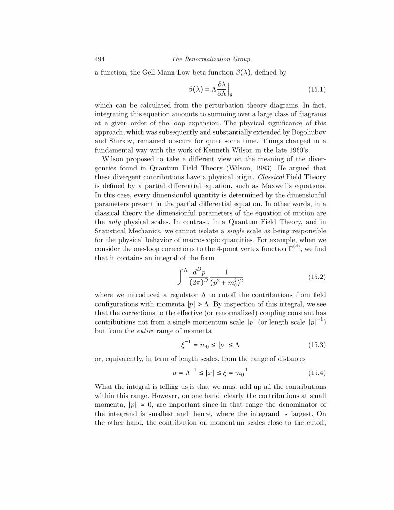
Wilson proposed to take a different view on the meaning of the diver-gencies found in Quantum Field Theory (Wilson, 1983). He argued thatthese divergent contributions have a physical origin. Classical Field Theoryis defined by a partial differential equation, such as Maxwell’s equations.In this case, every dimensionful quantity is determined by the dimensionfulparameters present in the partial differential equation. In other words, in aclassical theory the dimensionful parameters of the equation of motion arethe only physical scales. In contrast, in a Quantum Field Theory, and inStatistical Mechanics, we cannot isolate a single scale as being responsiblefor the physical behavior of macroscopic quantities. For example, when weconsider the one-loop corrections to the 4-point vertex function Γ(4), we findthat it contains an integral of the form
∫ Λ dDp(2π)D 1(p2 +m2
0)2 (15.2)
where we introduced a regulator Λ to cutoff the contributions from fieldconfigurations with momenta ∣p∣ > Λ. By inspection of this integral, we seethat the corrections to the effective (or renormalized) coupling constant hascontributions not from a single momentum scale ∣p∣ (or length scale ∣p∣−1)but from the entire range of momenta
ξ−1
= m0 ≤ ∣p∣ ≤ Λ (15.3)
or, equivalently, in term of length scales, from the range of distances
a = Λ−1
≤ ∣x∣ ≤ ξ = m−10 (15.4)
What the integral is telling us is that we must add up all the contributionswithin this range. However, on one hand, clearly the contributions at smallmomenta, ∣p∣ ≈ 0, are important since in that range the denominator ofthe integrand is smallest and, hence, where the integrand is largest. Onthe other hand, the contribution on momentum scales close to the cutoff,
15.1 Scale dependence in Quantum Field Theory and in Statistical Physics495
∣p∣ ≈ Λ, are even bigger since the phase space is growing by a factor ofΛD. Thus, we should expect divergencies to occur since there is no physicalmechanism to stop fluctuations on length scales between a short distancecutoff a and a macroscopic scale ξ from happening. It is important to notethat this sensitivity to the definition of the theory at short distances willstill be present even if local field theory is replaced at even shorter distancesby some other theory, perhaps more fundamental, such as String Theory.At any rate, in all cases, there will remain a sensitivity on the definition ofthe theory at some short-distance scale used to define the local field theory.We will see shortly that these very same issues arise in the theory of phasetransitions in Statistical Physics.
In Quantum Field Theory, in Euclidean space time, the N -point functionsare given in terms of the path integral which for a scalar field φ has the form
Z[J] = ∫ Dφ e−SΛ[φ]+∫ d
DxJφ
(15.5)
where SΛ[φ] is the Euclidean action for a theory defined with a regulatorΛ = a
−1. To define a theory without a regulator amounts to take the limitΛ → ∞ or, equivalently, to take the limit in which short-distance cutoffa → 0. If one regards the short-distance cutoff as a lattice spacing, this isthe same as defining a continuum limit.
In some sense, the procedure of removing the UV regulator from a fieldtheory is reminiscent to the definition the integral of a real function on afinite interval as the limit of a Riemann sum. However, while in the case ofthe integral the limit exists, provided the function has bounded variation,in the case of a functional integral the problem is much more complex. Theproblem of defining a field theory without a regulator is then reduced tounderstand when, and how, it is possible to take such a limit. One canregard the field theory as being defined with a UV cutoff a, e.g., the “latticespacing”, and define a process of taking the continuum limit as the limit ofa sequence of theories defined at progressively smaller UV length scales, sayfrom scale a = Λ−1, to a
2=
2Λ, to a
4=
4Λ, etc. In each step, the number of
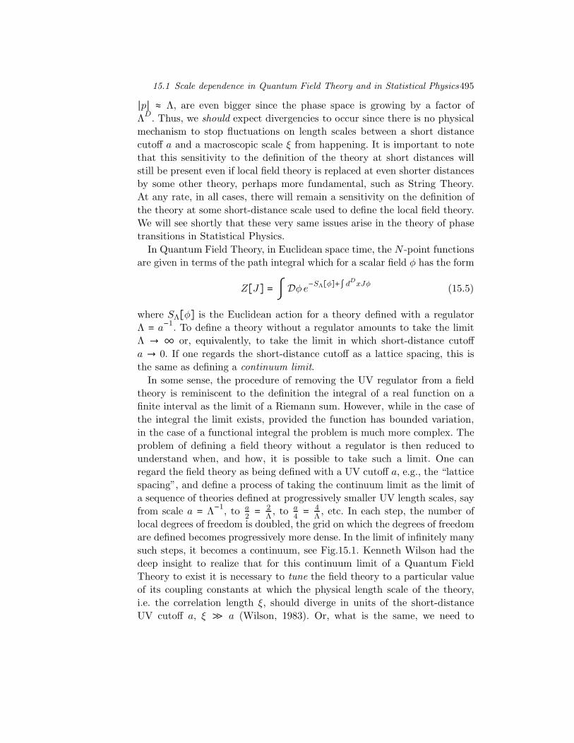
local degrees of freedom is doubled, the grid on which the degrees of freedomare defined becomes progressively more dense. In the limit of infinitely manysuch steps, it becomes a continuum, see Fig.15.1. Kenneth Wilson had thedeep insight to realize that for this continuum limit of a Quantum FieldTheory to exist it is necessary to tune the field theory to a particular valueof its coupling constants at which the physical length scale of the theory,i.e. the correlation length ξ, should diverge in units of the short-distanceUV cutoff a, ξ ≫ a (Wilson, 1983). Or, what is the same, we need to
496 The Renormalization Group
a a
2
a
4
Figure 15.1 Taking the continuum limit: in each step the number of degreesof freedom is doubled, the UV scale a is halved, and the grid becomesprogressively denser.
find a regime in which the mass gap M = ξ−1 is much smaller than the
UV momentum cutoff Λ, M ≪ Λ. Phrased in this fashion, the problem ofdefining a quantum field theory is reduced to finding a regime in which thephysical correlation length is divergent. However, as we saw before, this is thesame as the problem of finding a continuous phase transition in StatisticalPhysics!. Thus, both problems are equivalent!
15.2 RG flows, fixed points and universality
In parallel, but independently from these developments of these ideas inQuantum Field Theory, the problem of the behavior of physical systemsnear a continuous phase transition was being reexamined and developed byseveral people, notably by Widom (Widom, 1965) and Fisher (Fisher, 1967),Patashinskii and Pokrovsky (Patashinskii and Pokrovskii, 1966), and, par-ticularly, by Kadanoff (Kadanoff, 1966). Near a continuous phase transition,“second order” in Landau’s terminology, certain physical quantities such asthe specific heat and the magnetic susceptibility, for a phase transition ina magnet, should generally be divergent as the critical temperature, Tc, isapproached. At Tc, the correlation length should be divergent. Using phe-nomenological arguments, they realized that that these properties can dedescribed by a singular contribution to the free energy density fsing, thathas a scaling form, i.e. a homogeneous function of the reduced temperature,t = (T − Tc)/Tc, and of the external magnetic field H (in dimensionlessunits). Implicit in these assumptions was the at the critical temperature Tc,where the correlation length diverges, the system exhibits scaling or, whatis the same, the system acquired an emergent symmetry: scale invariance.
Kadanoff formulated these ideas in terms of the following physically intu-itive picture (Kadanoff, 1966). Consider for instance the simplest model ofa magnet, the Ising model on a square lattice of spacing a. On each site one
15.2 RG flows, fixed points and universality 497
has an Ising spin: a degree of freedom that can take only two values, σ = ±1.The partition function of this problem is a sum over all the configurationsof spins, [σ], weighed by the Boltzmann probability for each configurationat temperature T
Z = ∑[σ]
exp(−S[σ]/T ) (15.6)
In the Ising model, the Euclidean action S[σ] is just the interaction energyof the spins,
S[σ] = −J ∑<i,j>
σ(i)σ(j) (15.7)
where < i, j > are nearest neighboring sites of the lattice, J is an energyscale (the exchange constant) and T is the temperature. In what follows,the energy of the classical statistical mechanical system will be called the“Euclidean action”.
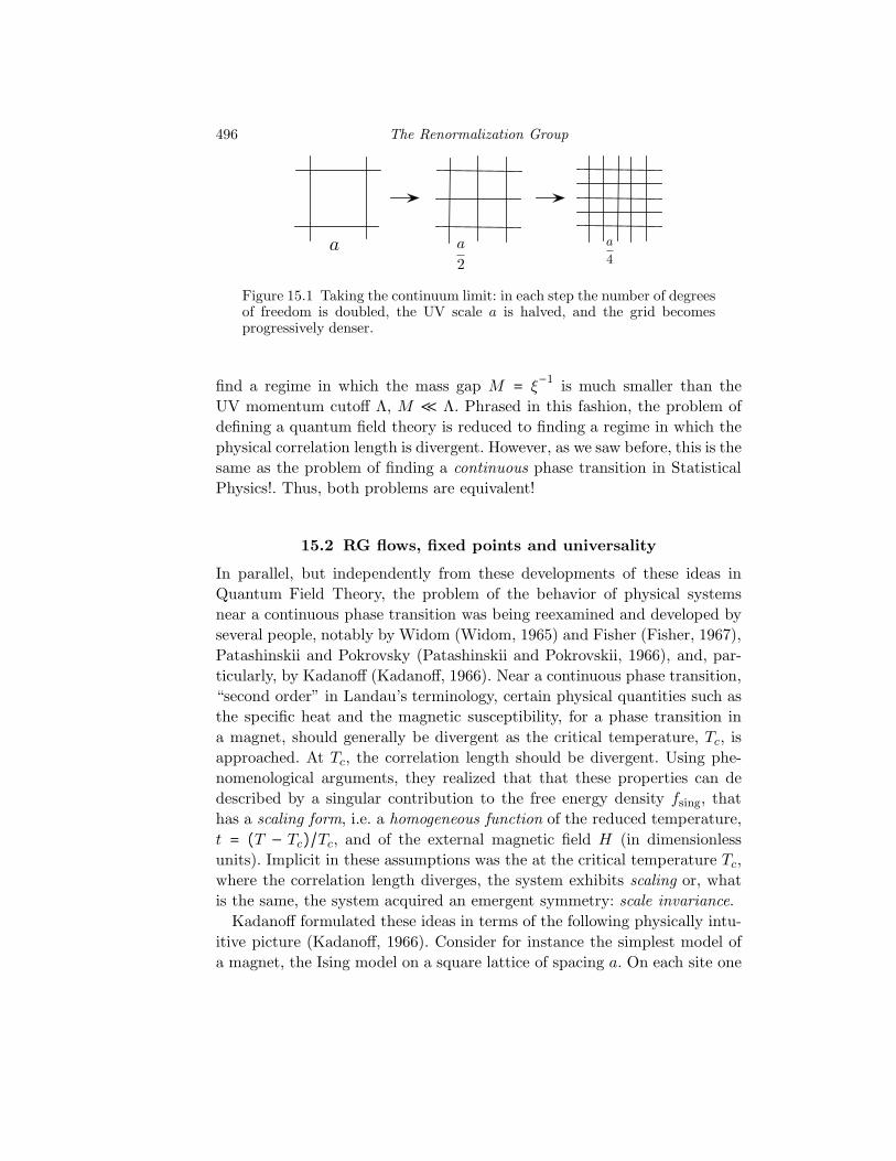
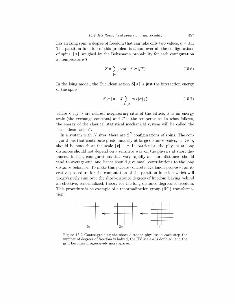
In a system with N sites, there are 2N configurations of spins. The con-figurations that contribute predominantly at large distance scales, ∣x∣ ≫ a,should be smooth at the scale ∣x∣ ∼ a. In particular, the physics at longdistances should not depend on a sensitive way on the physics at short dis-tances. In fact, configurations that vary rapidly at short distances shouldtend to average-out, and hence should give small contributions to the longdistance behavior. To make this picture concrete, Kadanoff proposed an it-erative procedure for the computation of the partition function which willprogressively sum over the short-distance degrees of freedom leaving behindan effective, renormalized, theory for the long distance degrees of freedom.This procedure is an example of a renormalization group (RG) transforma-tion.
a2a4a
Figure 15.2 Coarse-graining the short distance physics: in each step thenumber of degrees of freedom is halved, the UV scale a is doubled, and thegrid becomes progressively more sparse.
498 The Renormalization Group
15.2.1 Block-spin transformations
Beginning with a system with lattice spacing a, we will divide it into a set ofblock spins so that the new, coarse grained, system will have lattice spacing2a. We will then define a new effective spin for each block and compute theireffective Hamiltonian by tracing over (“integrating-out”) the the rapidlyvarying configurations at scale a. In effect, this is the same as the procedurefor the construction of the continuum field theory shown in Fig.15.1, exceptthat now we run the procedure backwards, from short distances to longdistances (see Fig.15.2). To this end, let us divide the system into cells, theblock spins, and let A be one of these cells. We define an effective degree offreedom µ for each cell
µ =∑i∈A σ(i)∣∣∑i∈A σ(i)∣∣ (15.8)
which represents the average over the configurations {σ} that vary rapidlyon the scale of the cell. Then the configurations on the block spins {µ},defined on a coarse-grained system with a new larger lattice spacing, say 2a,vary smoothly on short scales but not on long scales.
The next step is to define en effective Hamiltonian for the block spins {µ}through a block-spin transformation T [µ∣σ] such that
∑{µ}
T [µ∣σ] = 1 (15.9)
For example, one could take
T [µ∣σ] = δ (µ −∑i∈A σ(i)∣∣∑i∈A σ(i)∣∣) (15.10)
Once a specific transformation is chosen, the effective theory of the blockspins is obtained by inserting Eq.(15.9) in the partition function:
Z = ∑{σ}
e−S[σ]
= ∑{µ}
∑{σ}
T [µ∣σ] e−S[σ] (15.11)
which leads to the definition of an effective action, Seff[µ] of the block spins
e−Seff[µ]
= ∑{σ}
T [µ∣σ] e−S[σ] (15.12)
The partition function of the coarse-grained system is obviously the sameas that of the original system
Z = ∑{µ}
e−Seff[µ] (15.13)
15.2 RG flows, fixed points and universality 499
even though, in general, the actions are not, Seff[µ] ≠ S[σ]. As it is apparentfrom this formal discussion, the form of the effective action Seff dependson the block transformation chosen. Nevertheless, since Seff results fromsumming over the contributions of a finite subset of degrees of freedom, itis a finite expression that can be written in terms of a set of local operatorswith effective (renormalized) coefficients.
Thus this coarse-graining procedure maps a system with lattice spacing a
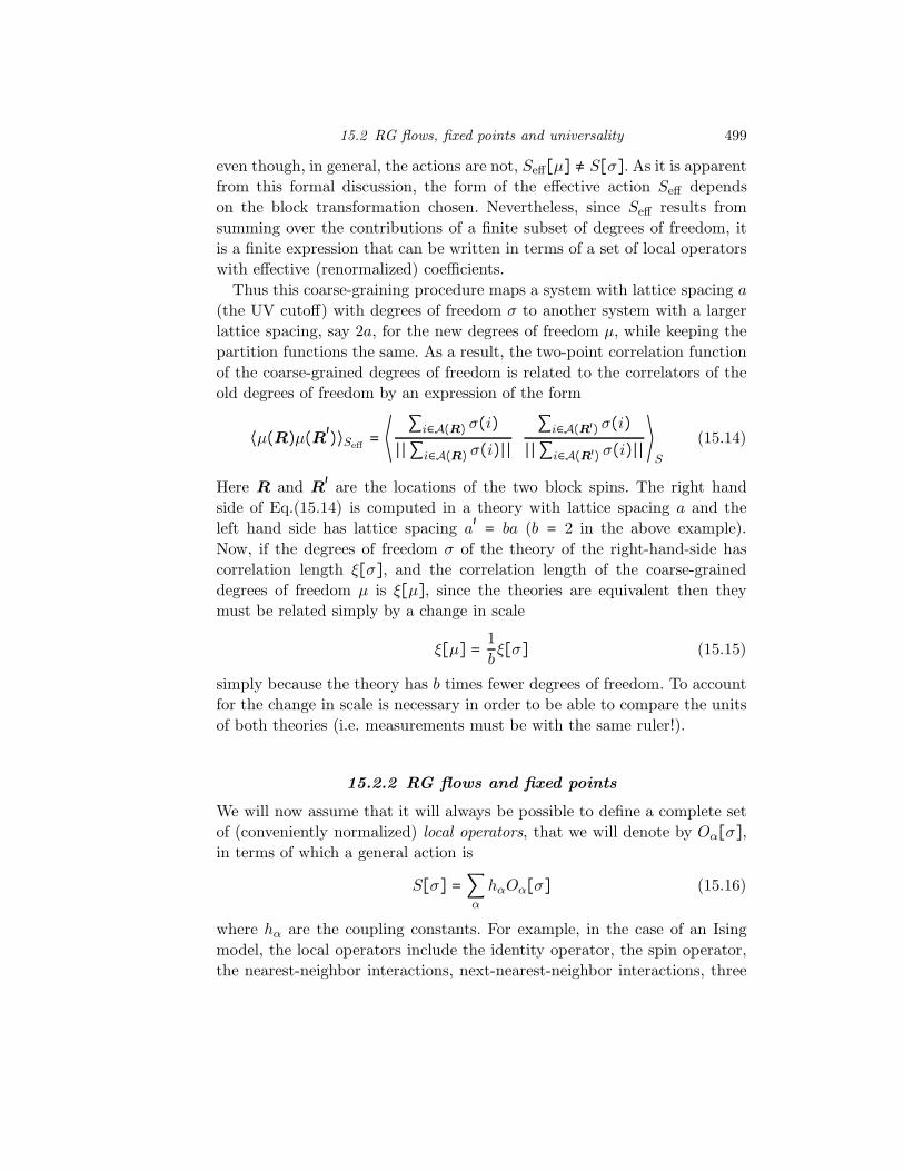
(the UV cutoff) with degrees of freedom σ to another system with a largerlattice spacing, say 2a, for the new degrees of freedom µ, while keeping thepartition functions the same. As a result, the two-point correlation functionof the coarse-grained degrees of freedom is related to the correlators of theold degrees of freedom by an expression of the form
⟨µ(R)µ(R′)⟩Seff= ⟨ ∑i∈A(R) σ(i)∣∣∑i∈A(R) σ(i)∣∣
∑i∈A(R′) σ(i)∣∣∑i∈A(R′) σ(i)∣∣⟩S (15.14)
Here R and R′ are the locations of the two block spins. The right hand
side of Eq.(15.14) is computed in a theory with lattice spacing a and theleft hand side has lattice spacing a
′= ba (b = 2 in the above example).
Now, if the degrees of freedom σ of the theory of the right-hand-side hascorrelation length ξ[σ], and the correlation length of the coarse-graineddegrees of freedom µ is ξ[µ], since the theories are equivalent then theymust be related simply by a change in scale
ξ[µ] = 1bξ[σ] (15.15)
simply because the theory has b times fewer degrees of freedom. To accountfor the change in scale is necessary in order to be able to compare the unitsof both theories (i.e. measurements must be with the same ruler!).
15.2.2 RG flows and fixed points
We will now assume that it will always be possible to define a complete setof (conveniently normalized) local operators, that we will denote by Oα[σ],in terms of which a general action is
S[σ] = ∑α
hαOα[σ] (15.16)
where hα are the coupling constants. For example, in the case of an Isingmodel, the local operators include the identity operator, the spin operator,the nearest-neighbor interactions, next-nearest-neighbor interactions, three
500 The Renormalization Group
and four spin interactions, etc. We will assume that the operators Oα[σ] arecomplete in a sense that we will specify below.
We will also assume that the theory of the corse-grained degrees of freedomµ is defined by the same set of local operators Oα[µ],
Seff[µ] = ∑α
heffα (b)Oα[µ] (15.17)
where heffα (b) are a set of renormalized interactions that depend on b = a′/a,
the change in the scale of the UV cutoff. The set of operators {Oα[σ]}is complete in the sense that its elements are the possible local operatorsgenerated under the RG transformation.
A consequence of this construction is that the coupling constants are nolonger fixed but are different at different scales. This result implies that theRG transformation induces a mapping in the space of coupling constants.The repeated action of the RG then can be viewed as a flow in this space:the RG flow.
Let us suppose, for the moment, that we have been clever enough to choosea transformation such that the renormalized couplings are related to the oldones by a homogeneous transformation of the scale, i.e.
heffα (b) = b
yαhα (15.18)
which, implicitly, includes a change in length scale. The exponents yα de-scribe how the couplings transform under the change of scale from a to ba.We now see that if the exponent yα > 0, then the coupling will be largerin the coarse-grained system (with scale ba), heffα > hα. Conversely, if theexponent yα < 0, then the coupling will be smaller in the coarse-grained sys-tem, heffα < hα. We will say that an operator for which yα > 0 is a relevantoperator while an operator with yα < 0 is an irrelevant operator. The RGflow of the coupling constant hα is given by the beta-function β(hα), whichin this context is defined as
β(hα) ≡ (heffα (b) − hα)/ ln b (15.19)
which measures the rate of change of the coupling hα for a logarithmicchange in the UV scale, ln b = ln(a′/a). For b → 1, the beta-function reducesto
β(hα) = ∂hα∂ ln b
= yαhα +O(h2α) (15.20)
which we will call the “tree-level” beta-function. The special case of yα = 0defines a marginal operator and the beta-function is given by higher orderterms that we have not yet included.
15.2 RG flows, fixed points and universality 501
It is now clear that if we keep repeating this transformation n times, thenin the limit n → ∞ the contribution of the irrelevant operators disappearsfrom the renormalized theory. In that limit, the Euclidean action of theeffective theory contains only marginal and relevant operators. FollowingWilson, we are led to conjecture that there should be theories which areinvariant under the action of these transformations, called renormalizationgroup transformations. Such theories are said to be fixed points of the renor-malization group, and we will denote their action by S
∗. Then, a genericrenormalized theory will have an Euclidean action of the form
S = S∗+∑
α
hα ∫ dDx Oα[σ(x)] (15.21)
which includes the fixed-point action, S∗, plus the set of, marginal and
relevant operators.The existence of theories described by such fixed points of the renormal-
ization group, conjectured by Wilson, is the key to understanding how todefine a quantum field theory. A theory described by such a fixed-point ac-tion S
∗ cannot depend on any microscopic scales, such as the UV cutoff (thelattice spacing a). Thus, at a fixed point there no scales left in the theory,and the theory becomes invariant under changes of scale, i.e. invariant underscale transformations. In order to achieve such a fixed point it is necessaryto rescale the lattice spacing ba of the renormalized theory described by Seff
back to what is was in the “bare” theory described by S. Hence, all lengthsmust be divided by b.
We summarize the construction of a renormalization group transformationby the following two steps: a) a block-spin (or coarse-graining) transforma-tion that eliminates a finite fraction of local degrees of freedom, followed byb) a rescaling of all lengths. We should note that an RG transformations isfor us to choose and different choices, i.e. different ways of averaging overthe short-distance physics, can always be made.
There are, as we noted, two types of fixed points depending on whetherthe correlation length is zero or infinite. Clearly, the short-distance physicscannot be eliminated from the theory if the fixed point has zero correlationlength. We will see that, in spite of this, such fixed points are importantsince they turn out to label the different possible phases (or types of vacuain field theory language) of a theory. One such example is a theory with aglobal symmetry in its spontaneously broken symmetry phase: the effectivefield theory of such a phase contains dimensionful quantities determined bythe physics at some short-distance scale.
On the other hand, if the fixed point has a divergent (infinite) correlation
502 The Renormalization Group
length, the definition of the theory at short distances should become irrel-evant at long distances, and the information on the short-distance physicsdisappears from a set of dimensionless quantities which, in this sense, becomeuniversal. This observation leads to the concept of the existence of universal-ity classes of theories which are characterized by fixed points with the sameuniversal properties. Once a fixed-point of this type can be reached, the the-ory has a new, emergent, symmetry: scale invariance. We will see shortlythat, under most circumstances of physical interest, it can be extended toan larger emergent symmetry: conformal invariance. Importantly, a theoryat a non-trivial fixed point and its set of marginal and relevant operatorsdefines a renormalizable quantum field theory. From this perspective, eachfixed pint (and, hence, each universality class) defines a different quantumfield theory.
Let us consider now some simple examples of RG flows and fixed points.We consider first a theory with a fixed point S∗ with one relevant pertur-
bation:
S = S∗+ h∫ d
Dx O[σ(x)] (15.22)
Under the RG with change of scale b = a′/a, we obtain
S′= S
∗+ b
yh∫ d
Dx O[µ(x)] (15.23)
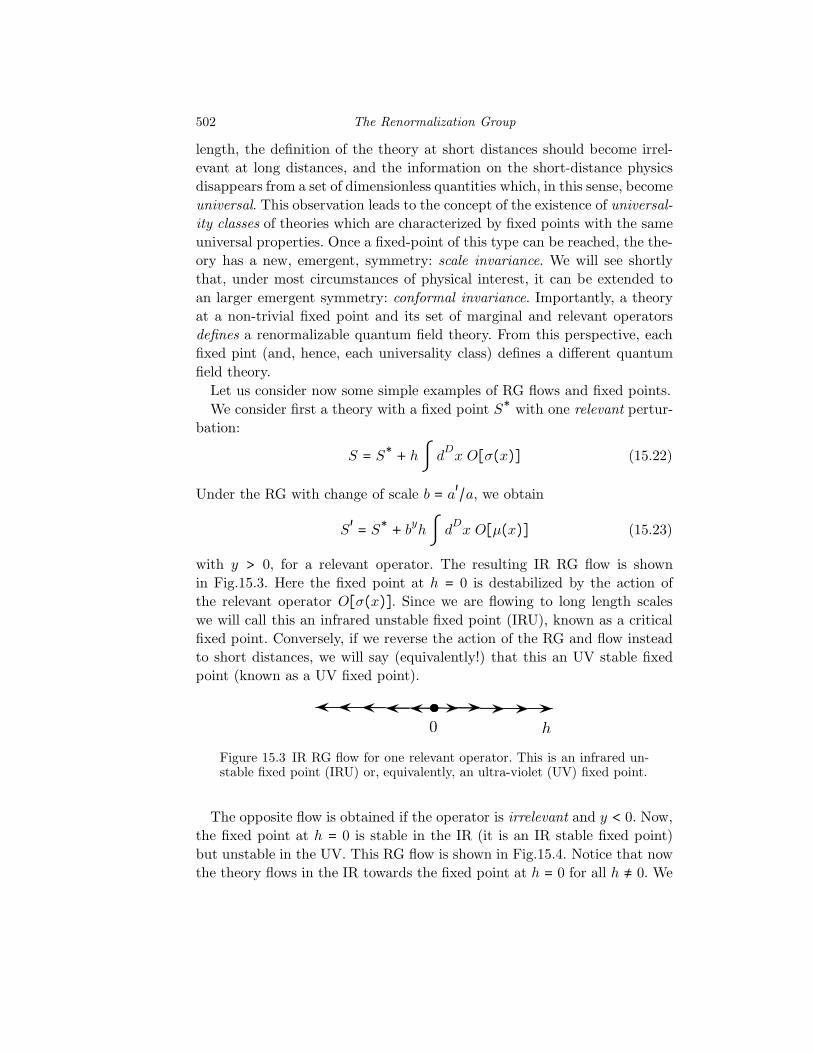
with y > 0, for a relevant operator. The resulting IR RG flow is shownin Fig.15.3. Here the fixed point at h = 0 is destabilized by the action ofthe relevant operator O[σ(x)]. Since we are flowing to long length scaleswe will call this an infrared unstable fixed point (IRU), known as a criticalfixed point. Conversely, if we reverse the action of the RG and flow insteadto short distances, we will say (equivalently!) that this an UV stable fixedpoint (known as a UV fixed point).
h0
Figure 15.3 IR RG flow for one relevant operator. This is an infrared un-stable fixed point (IRU) or, equivalently, an ultra-violet (UV) fixed point.
The opposite flow is obtained if the operator is irrelevant and y < 0. Now,the fixed point at h = 0 is stable in the IR (it is an IR stable fixed point)but unstable in the UV. This RG flow is shown in Fig.15.4. Notice that nowthe theory flows in the IR towards the fixed point at h = 0 for all h ≠ 0. We
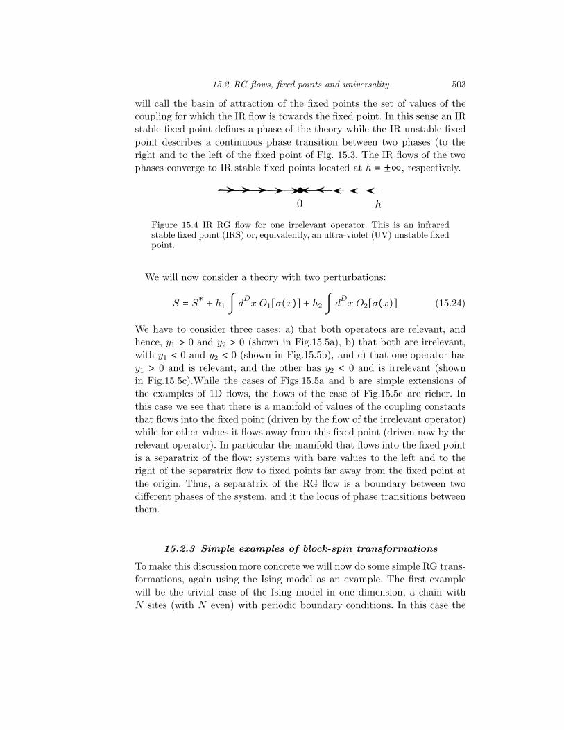
15.2 RG flows, fixed points and universality 503
will call the basin of attraction of the fixed points the set of values of thecoupling for which the IR flow is towards the fixed point. In this sense an IRstable fixed point defines a phase of the theory while the IR unstable fixedpoint describes a continuous phase transition between two phases (to theright and to the left of the fixed point of Fig. 15.3. The IR flows of the twophases converge to IR stable fixed points located at h = ±∞, respectively.
h0
Figure 15.4 IR RG flow for one irrelevant operator. This is an infraredstable fixed point (IRS) or, equivalently, an ultra-violet (UV) unstable fixedpoint.
We will now consider a theory with two perturbations:
S = S∗+ h1 ∫ d
Dx O1[σ(x)]+ h2 ∫ d
Dx O2[σ(x)] (15.24)
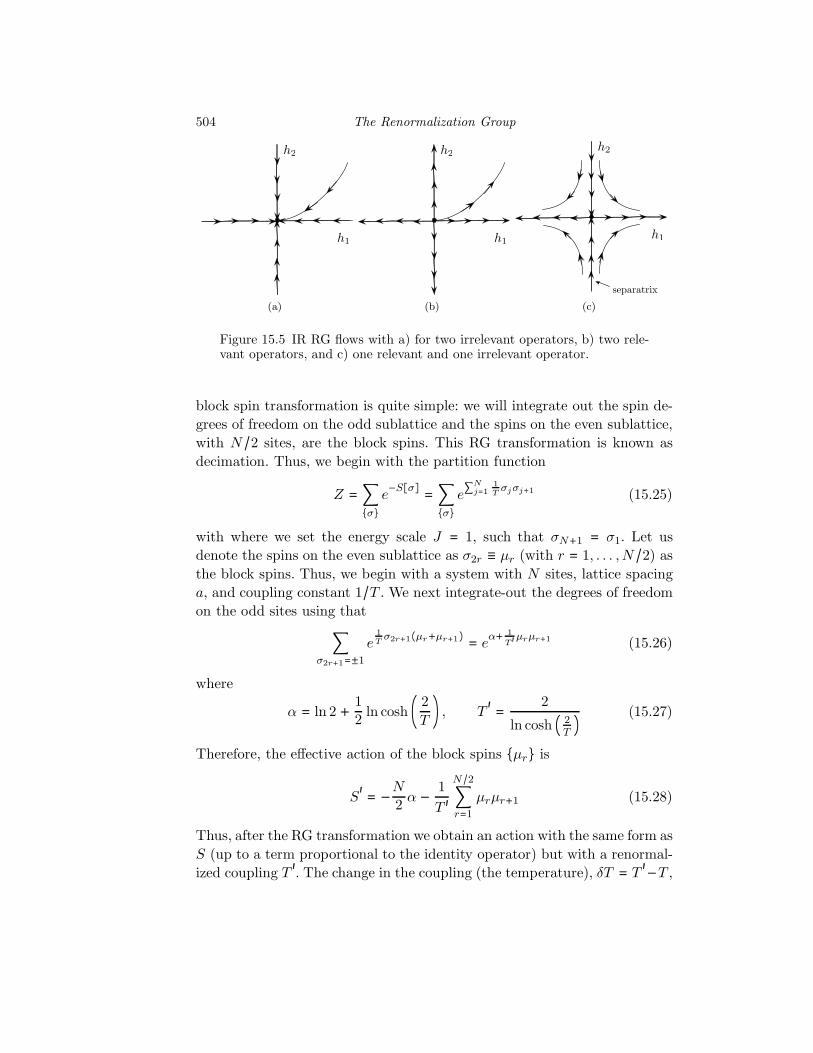
We have to consider three cases: a) that both operators are relevant, andhence, y1 > 0 and y2 > 0 (shown in Fig.15.5a), b) that both are irrelevant,with y1 < 0 and y2 < 0 (shown in Fig.15.5b), and c) that one operator hasy1 > 0 and is relevant, and the other has y2 < 0 and is irrelevant (shownin Fig.15.5c).While the cases of Figs.15.5a and b are simple extensions ofthe examples of 1D flows, the flows of the case of Fig.15.5c are richer. Inthis case we see that there is a manifold of values of the coupling constantsthat flows into the fixed point (driven by the flow of the irrelevant operator)while for other values it flows away from this fixed point (driven now by therelevant operator). In particular the manifold that flows into the fixed pointis a separatrix of the flow: systems with bare values to the left and to theright of the separatrix flow to fixed points far away from the fixed point atthe origin. Thus, a separatrix of the RG flow is a boundary between twodifferent phases of the system, and it the locus of phase transitions betweenthem.
15.2.3 Simple examples of block-spin transformations
To make this discussion more concrete we will now do some simple RG trans-formations, again using the Ising model as an example. The first examplewill be the trivial case of the Ising model in one dimension, a chain withN sites (with N even) with periodic boundary conditions. In this case the
504 The Renormalization Group
h1
h2
(a)
h1
h2
(b)
h1
h2
separatrix
(c)
Figure 15.5 IR RG flows with a) for two irrelevant operators, b) two rele-vant operators, and c) one relevant and one irrelevant operator.
block spin transformation is quite simple: we will integrate out the spin de-grees of freedom on the odd sublattice and the spins on the even sublattice,with N/2 sites, are the block spins. This RG transformation is known asdecimation. Thus, we begin with the partition function
Z = ∑{σ}
e−S[σ]
= ∑{σ}
e∑N
j=11Tσjσj+1 (15.25)
with where we set the energy scale J = 1, such that σN+1 = σ1. Let usdenote the spins on the even sublattice as σ2r ≡ µr (with r = 1, . . . , N/2) asthe block spins. Thus, we begin with a system with N sites, lattice spacinga, and coupling constant 1/T . We next integrate-out the degrees of freedomon the odd sites using that
∑σ2r+1=±1
e1Tσ2r+1(µr+µr+1)
= eα+ 1
T ′ µrµr+1 (15.26)
where
α = ln 2 +12ln cosh ( 2
T) , T
′=
2
ln cosh ( 2T) (15.27)
Therefore, the effective action of the block spins {µr} is
S′= −
N
2α −
1
T ′
N/2∑r=1
µrµr+1 (15.28)
Thus, after the RG transformation we obtain an action with the same form asS (up to a term proportional to the identity operator) but with a renormal-ized coupling T
′. The change in the coupling (the temperature), δT = T′−T ,
15.2 RG flows, fixed points and universality 505
for low values of T → 0, is given by the beta-function, β(T )β(T ) = δT
ln 2=
T2
2+O(T 3) (15.29)
where ln 2 = ln(a′/a) is the log of the change in the UV scale.At a fixed point, T∗, we must have T ′∗
= T∗ or, what is the same, δT∗
= 0.This clearly happens only at T = T
∗= 0. Hence, the only finite fixed point
(i.e., aside from T∗→ ∞) is at T
∗= 0. Moreover, since the beta-function
of Eq.(15.29) is always positive, the T∗= 0 fixed point is unstable and the
theory flows to the strong coupling fixed point at T∗→ ∞ for all T > 0.
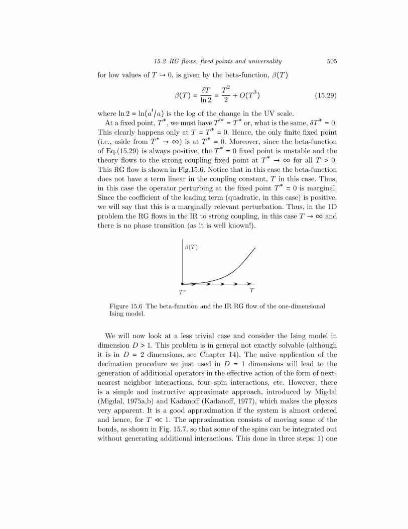
This RG flow is shown in Fig.15.6. Notice that in this case the beta-functiondoes not have a term linear in the coupling constant, T in this case. Thus,in this case the operator perturbing at the fixed point T
∗= 0 is marginal.
Since the coefficient of the leading term (quadratic, in this case) is positive,we will say that this is a marginally relevant perturbation. Thus, in the 1Dproblem the RG flows in the IR to strong coupling, in this case T → ∞ andthere is no phase transition (as it is well known!).
β(T )
TT ∗
Figure 15.6 The beta-function and the IR RG flow of the one-dimensionalIsing model.
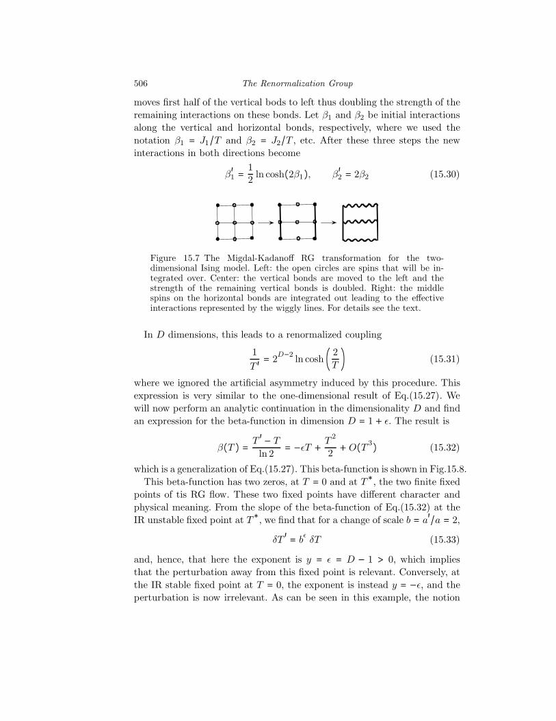
We will now look at a less trivial case and consider the Ising model indimension D > 1. This problem is in general not exactly solvable (althoughit is in D = 2 dimensions, see Chapter 14). The naive application of thedecimation procedure we just used in D = 1 dimensions will lead to thegeneration of additional operators in the effective action of the form of next-nearest neighbor interactions, four spin interactions, etc. However, thereis a simple and instructive approximate approach, introduced by Migdal(Migdal, 1975a,b) and Kadanoff (Kadanoff, 1977), which makes the physicsvery apparent. It is a good approximation if the system is almost orderedand hence, for T ≪ 1. The approximation consists of moving some of thebonds, as shown in Fig. 15.7, so that some of the spins can be integrated outwithout generating additional interactions. This done in three steps: 1) one
506 The Renormalization Group
moves first half of the vertical bods to left thus doubling the strength of theremaining interactions on these bonds. Let β1 and β2 be initial interactionsalong the vertical and horizontal bonds, respectively, where we used thenotation β1 = J1/T and β2 = J2/T , etc. After these three steps the newinteractions in both directions become
β′1 =
12ln cosh(2β1), β
′2 = 2β2 (15.30)
Figure 15.7 The Migdal-Kadanoff RG transformation for the two-dimensional Ising model. Left: the open circles are spins that will be in-tegrated over. Center: the vertical bonds are moved to the left and thestrength of the remaining vertical bonds is doubled. Right: the middlespins on the horizontal bonds are integrated out leading to the effectiveinteractions represented by the wiggly lines. For details see the text.
In D dimensions, this leads to a renormalized coupling
1
T ′= 2
D−2ln cosh ( 2
T) (15.31)
where we ignored the artificial asymmetry induced by this procedure. Thisexpression is very similar to the one-dimensional result of Eq.(15.27). Wewill now perform an analytic continuation in the dimensionality D and findan expression for the beta-function in dimension D = 1 + ϵ. The result is
β(T ) = T′− T
ln 2= −ϵT +
T2
2+O(T 3) (15.32)
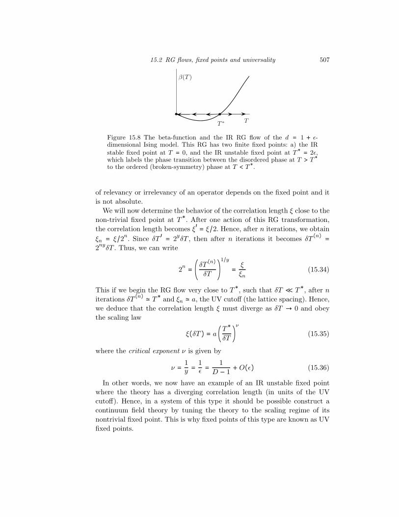
which is a generalization of Eq.(15.27). This beta-function is shown in Fig.15.8.This beta-function has two zeros, at T = 0 and at T∗, the two finite fixed
points of tis RG flow. These two fixed points have different character andphysical meaning. From the slope of the beta-function of Eq.(15.32) at theIR unstable fixed point at T∗, we find that for a change of scale b = a
′/a = 2,
δT′= b
ϵδT (15.33)
and, hence, that here the exponent is y = ϵ = D − 1 > 0, which impliesthat the perturbation away from this fixed point is relevant. Conversely, atthe IR stable fixed point at T = 0, the exponent is instead y = −ϵ, and theperturbation is now irrelevant. As can be seen in this example, the notion
15.2 RG flows, fixed points and universality 507
β(T )
TT ∗
Figure 15.8 The beta-function and the IR RG flow of the d = 1 + ϵ-dimensional Ising model. This RG has two finite fixed points: a) the IRstable fixed point at T = 0, and the IR unstable fixed point at T
∗= 2ϵ,
which labels the phase transition between the disordered phase at T > T∗
to the ordered (broken-symmetry) phase at T < T∗.
of relevancy or irrelevancy of an operator depends on the fixed point and itis not absolute.
We will now determine the behavior of the correlation length ξ close to thenon-trivial fixed point at T
∗. After one action of this RG transformation,the correlation length becomes ξ′ = ξ/2. Hence, after n iterations, we obtain
ξn = ξ/2n. Since δT ′= 2yδT , then after n iterations it becomes δT (n)
=
2nyδT . Thus, we can write
2n= (δT (n)
δT)1/y =
ξ
ξn(15.34)
This if we begin the RG flow very close to T∗, such that δT ≪ T
∗, after niterations δT (n)
≃ T∗ and ξn ≃ a, the UV cutoff (the lattice spacing). Hence,
we deduce that the correlation length ξ must diverge as δT → 0 and obeythe scaling law
ξ(δT ) = a (T∗
δT)ν (15.35)
where the critical exponent ν is given by
ν =1y =
1ϵ =
1D − 1
+O(ϵ) (15.36)
In other words, we now have an example of an IR unstable fixed pointwhere the theory has a diverging correlation length (in units of the UVcutoff). Hence, in a system of this type it should be possible construct acontinuum field theory by tuning the theory to the scaling regime of itsnontrivial fixed point. This is why fixed points of this type are known as UVfixed points.
508 The Renormalization Group
15.2.4 The Wilson-Fisher momentum-shell RG
We will now look at a different type of RG transformation: the momen-tum shell RG introduced by Kenneth Wilson and Michael Fisher (Wilsonand Fisher, 1972). Instead of blocks of local degrees of freedom, we willfocus on momentum space and we will integrate-out progressively the high-momentum modes of the field configurations (Wilson and Kogut, 1974).Here we will focus on the case of the Euclidean φ4 theory, which is a equiv-alent to the Landau-Ginzburg theory of phase transitions. The action in D
Euclidean dimensions is
S = ∫ dDx [1
2(∂µφ)2 + t
2Λ2φ2+
u
4!Λϵφ4] (15.37)
where we have defined the mass m20 and the coupling constant λ in terms of
the UV cutoff Λ as m20 = tΛ2 and λ = uΛϵ, where t and u are dimensionless
and ϵ = 4 −D.
This approach begins by splitting the field into slow and fast components,denoted by φ< and φ>, respectively,
φ(x) = φ<(x) + φ>(x) (15.38)
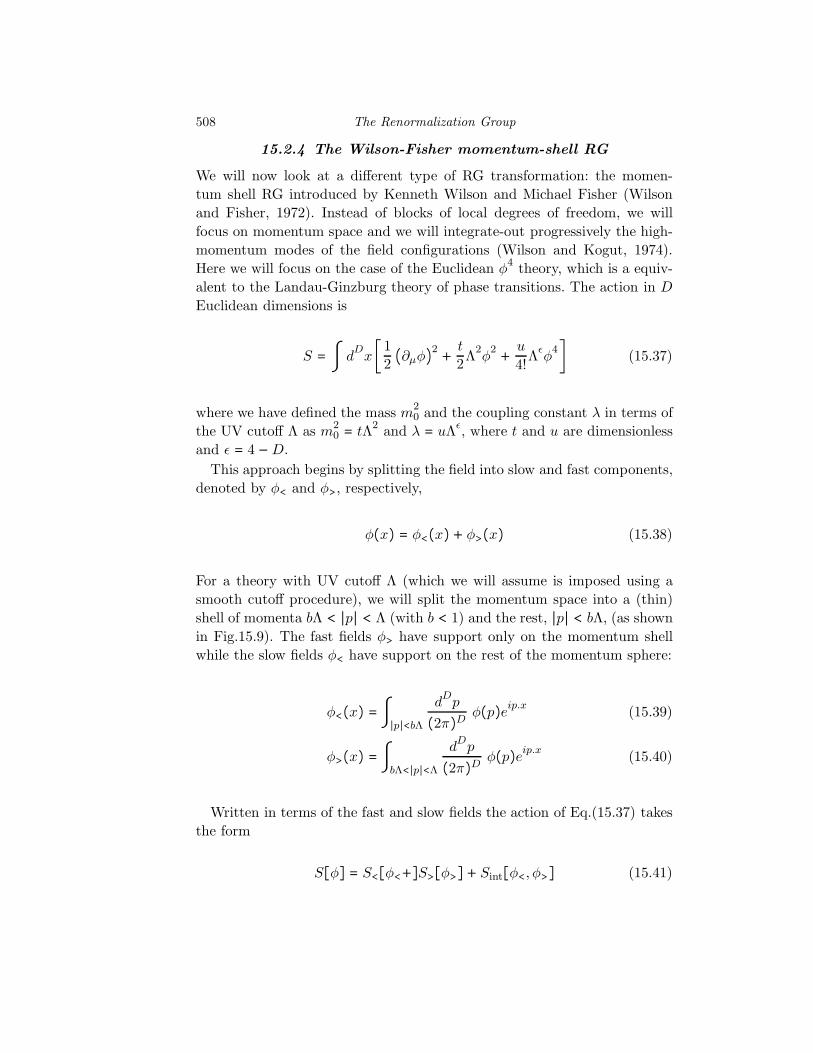
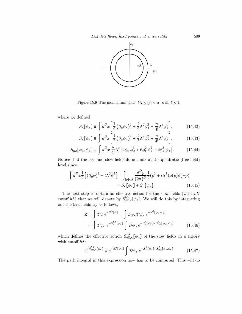
For a theory with UV cutoff Λ (which we will assume is imposed using asmooth cutoff procedure), we will split the momentum space into a (thin)shell of momenta bΛ < ∣p∣ < Λ (with b < 1) and the rest, ∣p∣ < bΛ, (as shownin Fig.15.9). The fast fields φ> have support only on the momentum shellwhile the slow fields φ< have support on the rest of the momentum sphere:
φ<(x) =∫∣p∣<bΛdDp(2π)D φ(p)eip.x (15.39)
φ>(x) =∫bΛ<∣p∣<Λ
dDp(2π)D φ(p)eip.x (15.40)
Written in terms of the fast and slow fields the action of Eq.(15.37) takesthe form
S[φ] = S<[φ<+]S>[φ>] + Sint[φ<,φ>] (15.41)
15.2 RG flows, fixed points and universality 509
py
px
ΛbΛ
Figure 15.9 The momentum shell, bΛ < ∣p∣ < Λ, with b < 1.
where we defined
S<[φ<] ≡∫ dDx [1
2(∂µφ<)2 + t
2Λ2φ2< +
u
4!Λϵφ4<] , (15.42)
S<[φ>] ≡∫ dDx [1
2(∂µφ>)2 + t
2Λ2φ2> +
u
4!Λϵφ4>] , (15.43)
Sint[φ<,φ>] ≡∫ dDx
u
4!Λϵ [4φ> φ3< + 6φ
2> φ
2< + 4φ
3> φ<] . (15.44)
Notice that the fast and slow fields do not mix at the quadratic (free field)level since
∫ dDx12[(∂µφ)2 + tΛ
2φ2] =∫∣p∣<Λ
dDp(2π)D 1
2(p2 + tΛ
2)φ(p)φ(−p)=S<[φ<]+ S>[φ>] (15.45)
The next step to obtain an effective action for the slow fields (with UVcutoff bΛ) that we will denote by S
bΛeff ,<[φ<]. We will do this by integrating
out the fast fields φ> as follows,
Z =∫ Dφ e−S
Λ[φ]= ∫ Dφ<Dφ> e
−SΛ[φ>,φ<]
=∫ Dφ< e−S
bΛ< [φ<] ∫ Dφ> e
−SΛ> [φ>]−SΛ
int[φ> ,φ<] (15.46)
which defines the effective action SbΛeff ,<[φ<] of the slow fields in a theory
with cutoff bΛ:
e−S
bΛeff,<[φ<]
≡ e−S
Λ< [φ<] ∫ Dφ> e
−SΛ> [φ>]−SΛ
int[φ>,φ<] (15.47)
The path integral in this expression now has to be computed. This will do
510 The Renormalization Group
using perturbation theory in u, which is equivalent to working at one looporder in the fluctuations if the fast fields. To this end we write the action ofthe fast fields as a sum of a massive free fast field action and an interactionterm,
SΛ> [φ>] = S
Λ0,>[φ>]+ S
Λint,>[φ>] (15.48)
We find
∫ Dφ> e−S
Λ> [φ>]−SΛ
int[φ>,φ<]=Z0,>
∞
∑n=0
(−1)nn!
(−uΛϵ
4!)n In[φ<] (15.49)
where Z0,> = exp(−F 0>) is the partition function for free fast fields defined
in the momentum shell, and where de define In[φ<] as
In[φ<] = ∫{xj} ⟨n
∏j=1
[φ4>(xj) + 4φ3>(xj)φ<(xj) + 6φ
2>(xj)φ2<(xj)
+4φ>(xj)φ3<(xj)]⟩0,>
(15.50)
where ⟨. . .⟩0,> represents an expectation value on the free fast fields. We
will use below that, symmetry, ⟨φ2k+1> (x)⟩0,> = 0, which applies to the ex-pectation values of similar expectation values of odd numbers of fast fieldoperators.
To first (lowest) order in u we find
I1 = ∫ dDx [⟨φ4>(x)⟩0,> + 6⟨φ2>(x)⟩0,>φ2<(x)] (15.51)
Similarly, we find that I2 is given by the expression
I2[φ<] = ∫ dDx1 ∫ d
Dx2[⟨φ4>(x1)φ4>(x2)⟩0,> + 12⟨φ4>(x1)φ2>(x2)⟩0,>φ2<(x2)
+ 16⟨φ3>(x1)φ3>(x2)⟩0,>φ<(x1)φ<(x2)+ 36⟨φ2>(x1)φ2>(x2)⟩0,>φ2<(x1)φ2<(x2)+ 16⟨φ>(x1)φ>(x2)⟩0,>φ3<(x1)φ3<(x2)+ 32⟨φ3>(x1)φ>(x2)⟩0,>φ<(x1)φ3<(x2)] (15.52)
Using these results we find that, up to cubic order in the dimensionlesscoupling constant u, the effective action S
bΛeff ,<[φ<] is
SbΛeff ,<[φ<] = S
bΛ< [φ<] + (uΛϵ
4!) I1 − 1
2!(uΛϵ
4!)2 (I2 − I
21)+O(u3) (15.53)
15.2 RG flows, fixed points and universality 511
where I1 and I2 are given in Eq.(15.51) and Eq.(15.52), respectively. Theexplicit form of the effective action is
SbΛeff ,<[φ<] = ∫ d
Dx[1
2(∂µφ<)2 + t
2Λ2φ2< +
u
4!Λϵφ4<]
+[F 0> + (uΛϵ
4!)∫ d
Dx⟨φ4>(x)⟩0,> −
12(uΛϵ
4!)2 ∫
x1,x2
⟨∶ φ4>(x1) ∶∶ φ4>(x2) ∶⟩>,0]+{ (uΛϵ
4!)∫ d
Dx 6⟨φ2>(x)⟩>,0φ2<(x)
−12(uΛϵ
4!)2 ∫
x1,x2
[36⟨∶ φ2>(x1) ∶∶ φ2>(x2) ∶⟩>,0φ2<(x1)φ2<(x2)+ 12⟨∶ φ4>(x1) ∶∶ φ2>(x2) ∶⟩>,0φ2<(x2) + 16⟨φ>(x1)φ>(x2)⟩>,0φ3<(x1)φ3<(x2)+ 16⟨φ3>(x1)φ3>(x2)⟩>,0φ<(x1)φ<(x2) + 32⟨φ3>(x1)φ>(x2)⟩>,0φ<(x1)φ3<(x2)]+O(u3)} (15.54)
where F0> = − lnZ0,>, and where we used the notation ∶ A ∶= A− ⟨A⟩0,> for
the normal ordered operator A with respect to the fast free field theory.We will now write the expression for the effective action for the slow fields
in terms of a set of local operators of the form φn< and derivatives, e.g. ∂i∂jφ
n<,
etc. We can do that since the kernels that appear in Eq.(15.54) involve onlythe correlators of the fast fields which are rapidly decaying functions of thecoordinates (provided the cutoff function used to restrict the fields to themomentum shell are smooth).
Let us consider for example the contribution
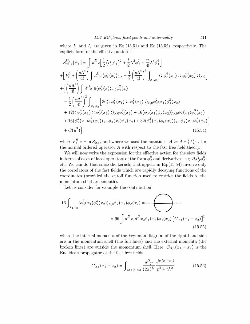
16∫x1,x2
⟨φ3>(x1)φ3>(x2)⟩>,0φ<(x1)φ<(x2) == 96∫ d
Dx1d
Dx2φ<(x1)φ<(x2) [G0,>(x1 − x2)]3
(15.55)
where the internal momenta of the Feynman diagram of the right hand sideare in the momentum shell (the full lines) and the external momenta (thebroken lines) are outside the momentum shell. Here, G0,>(x1 − x2) is theEuclidean propagator of the fast free fields
G0,>(x1 − x2) = ∫bΛ<∣p∣<Λ
dDp(2π)D e
ip⋅(x1−x2)p2 + tΛ2 (15.56)
512 The Renormalization Group
We will assume that the cutoff implied by the restriction to the momentumshell is smooth enough so that this propagator decays exponentially withdistance. Under these assumptions, it is legitimate perform inside the inte-gral shown in Eq.(15.55) a Taylor expansion of the slow field φ<(x2) aboutthe coordinate x1:
φ<(x2) = φ<(x2+ ℓ) = φ<(x1)+ ℓi∂iφ<(x1)+ 12ℓiℓj∂i∂jφ<(x1)+ . . . (15.57)
We can then write the integral in right hand side of Eq.(15.55) as
∫ dxD1 dx
D2 φ<(x1)φ<(x2) [G0,>(x1 − x2)]3 =
=∫ dDx φ
2<(x)∫ d
Dℓ [G0,>(ℓ)]3 − 1
D[∫ d
Dℓ ℓ
2 [G0,>(ℓ)]3] 12(∂µφ<(x))2 + . . .
(15.58)
Therefore, the contribution of Eq.(15.55) is part of the mass renormalizationand of the wave function renormalization.
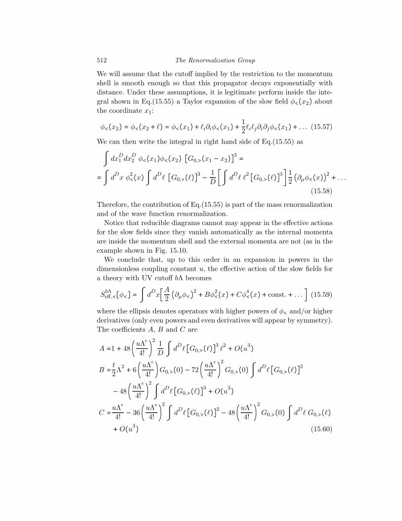
Notice that reducible diagrams cannot may appear in the effective actionsfor the slow fields since they vanish automatically as the internal momentaare inside the momentum shell and the external momenta are not (as in theexample shown in Fig. 15.10.
We conclude that, up to this order in an expansion in powers in thedimensionless coupling constant u, the effective action of the slow fields fora theory with UV cutoff bΛ becomes
SbΛeff,<[φ<] = ∫ d
Dx[A
2(∂µφ<)2 +Bφ
2<(x)+Cφ
4<(x)+ const.+ . . . ] (15.59)
where the ellipsis denotes operators with higher powers of φ< and/or higherderivatives (only even powers and even derivatives will appear by symmetry).The coefficients A, B and C are
A =1 + 48 (uΛϵ4!
)2 1D
∫ dDℓ [G0,>(ℓ)]3 ℓ2 +O(u3)
B =t
2Λ2+ 6 (uΛϵ
4!)G0,>(0) − 72 (uΛϵ
4!)2 G0,>(0)∫ d
Dℓ [G0,>(ℓ)]2
− 48 (uΛϵ4!
)2 ∫ dDℓ [G0,>(ℓ)]3 +O(u3)
C =uΛϵ
4!− 36 (uΛϵ
4!)2 ∫ d
Dℓ [G0,>(ℓ)]2 − 48 (uΛϵ
4!)2G0,>(0)∫ d
Dℓ G0,>(ℓ)
+O(u3) (15.60)
15.2 RG flows, fixed points and universality 513
Here we ignored the constant terms, which are a contribution to the renor-malization of the identity operator.
The remaining integrals can be done quite easily. In the limit in which theshell is very thin (compared to the cutoff scale Λ), and writing b = e
−δs→ 1−
as δs → 0+, the integrals become
G0,>(0) =∫shell
dDp(2π)D 1
p2 + tΛ2 =ΛD−2
1 + t
SD(2π)D δs∫ d
Dℓ G0,>(ℓ) =∫
shell
dDp(2π)D (2π)DδD(p)
p2 + tΛ2 = 0
∫ dDℓ [G0,>(ℓ)]2 = ΛD−4
(1 + t)2 SD(2π)D δs∫ d
Dℓ [G0,>(ℓ)]3 = Λ2D−6
(1 + t)3 SD(2π)D δs∫ d
Dℓ [G0,>(ℓ)]3 ℓ2 =Λ2D−8 [ 2D(1 + t)4 −
8(1 + t)5 ] SD(2π)D δs (15.61)
where
SD =2πD/2Γ(D/2) (15.62)
is the area of the hypersphere, and Γ(x) is the Gamma function.
Figure 15.10 Reducible Feynman diagrams with internal momenta in themomentum shell vanish identically by momentum conservation.
The last step is to define a rescaled field
φ′= Z
−1/2φ φ< (15.63)
which we readily identify with the wave function renormalization, and torescale the coordinates,
x′= bx (15.64)
so that the cutoff scale in the new rescaled coordinates in back to Λ. The
514 The Renormalization Group
resulting action for the (rescaled) field φ′ in the rescaled coordinates x′ is
S′(φ′) =SbΛ
eff,<(φ<)=∫ d
Dx′b−D[A
2Zφb
2 (∂′µφ′)2 +BZφφ′2+ CZ
2φφ
′4] (15.65)
and we will require that the renormalization conditions
1 =b2−D
AZφ (15.66)
t′
2Λ2=b
−DBZφ (15.67)
u′
4!Λϵ=b
−DCZ
2φ (15.68)
be satisfied. By keeping only the leading corrections to t and u, we obtain
Zφ =bD−2
A−1
= bD−2 (1 +O(u2))]) (15.69)
t′=b
−2 [t + 12(u − ut) SD(2π)D δs +O(u2, t2)] (15.70)
u′=b
−ϵ [u −32u2 SD(2π)D δs +O(u3, t2)] (15.71)
Notice that, at this leading order, the wave function renormalization is triv-ial. Also notice the important fact that all dependence from the momentumcutoff scale Λ has cancelled exactly. This is a generic feature of RG trans-formations. Finally, these equations simplify if we absorb the phase spacefactors in a new dimensionless coupling constant v
v = uSD(2π)D (15.72)
The (Gell-Mann-Low) beta-functions for the dimensionless couplings t
and v are defined to be
βt =dt
ds=a
dt
da= −Λ
dt
dΛ
βv =dv
ds=a
dv
da= −Λ
dv
dΛ(15.73)
Using the results we just derived, we find that the beta-functions are
βt =2t +v
2−
12vt + . . . (15.74)
βv =ϵv −32v2+ . . . (15.75)
to leading orders in the couplings t and v, and in ϵ = 4 − D. Therefore,
15.2 RG flows, fixed points and universality 515
this perturbative RG transformation, is accurate only to order ϵ, and is thebeginning of a series in powers of ϵ. This is the ϵ-expansion (Wilson andKogut, 1974).
D < 4
WF
G
u
β(u)
(a)
G
u
β(u)
(b)
WF
G
t
u
(c)
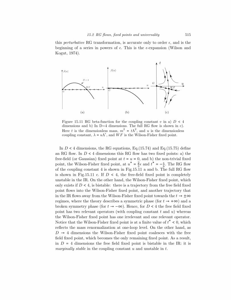
Figure 15.11 RG beta-function for the coupling constant v in a) D < 4dimensions and b) In D=4 dimensions. The full RG flow is shown in c).Here t is the dimensionless mass, m2
= tΛ2, and u is the dimensionlesscoupling constant, λ = uΛϵ, and WF is the Wilson-Fisher fixed point.
In D < 4 dimensions, the RG equations, Eq.(15.74) and Eq.(15.75) definean RG flow. In D < 4 dimensions this RG flow has two fixed points: a) thefree-field (or Gaussian) fixed point at t = u = 0, and b) the non-trivial fixedpoint, the Wilson-Fisher fixed point, at u∗ =
23ϵ and t
∗= − ϵ
6. The RG flow
of the coupling constant 4 is shown in Fig.15.11 a and b. The full RG flowis shown in Fig.15.11 c. If D < 4, the free-field fixed point is completelyunstable in the IR. On the other hand, the Wilson-Fisher fixed point, whichonly exists if D < 4, is bistable: there is a trajectory from the free field fixedpoint flows into the Wilson-Fisher fixed point, and another trajectory thatin the IR flows away from the Wilson-Fisher fixed point towards the t → ±∞
regimes, where the theory describes a symmetric phase (for t → +∞) and abroken symmetry phase (for t → −∞). Hence, for D < 4 the free field fixedpoint has two relevant operators (with coupling constant t and u) whereasthe Wilson-Fisher fixed point has one irrelevant and one relevant operator.Notice that the Wilson-Fisher fixed point is at a finite value of t∗ < 0, whichreflects the mass renormalization at one-loop level. On the other hand, asD → 4 dimensions the Wilson-Fisher fixed point coalesces with the freefield fixed point, which becomes the only remaining fixed point. As a result,in D = 4 dimensions the free field fixed point is bistable in the IR: it ismarginally stable in the coupling constant u and unstable in t.
516 The Renormalization Group
The RG flow for the coupling constants determines the behavior of thecorrelation length ξ. By dimensional analysis we can always write ξ in theform
ξ = Λ−1f(t, u) (15.76)
where f(t, u) is a dimensionless function of t and u. Consider now two phys-ical systems defined with different values of of the UV scale Λ but with thesame value of the physical scale ξ. Since ξ is fixed, we can write
0 =∂ξ
∂Λ= −Λ
−2f(t, u) + Λ
−1 ∂f
∂Λ(15.77)
However, f(t, u) does not depend explicitly on Λ but it depends implicitlyon the scale through the RG flow. Hence,
∂f
∂Λ=∂f
∂u
∂u
∂Λ+∂f
∂t
∂t
∂Λ(15.78)
By using the definitions of the beta-functions we find that the functionf(t, u) must obey the partial differential equation
f +∂f
∂uβu +
∂f
∂tβt = 0 (15.79)
This is an example of a Callan-Symanzik equation.We will solve Eq.(15.79) for the unstable trajectory of the Wilson-Fisher
fixed point. Close to the fixed point we can work with the linearized flowexpressed in terms of the variables x and y,
x = 4(t − t∗) + (1− ϵ
6) (v − v
∗), y = v − v∗
(15.80)
where (v∗, t∗) is the location of the Wilson-Fisher fixed point. The linearizedbeta-functions are
βx = (2 − ϵ
3)x + . . . , βy = −ϵy + . . . (15.81)
In these coordinates the fixed point is at (0, 0). Since the flow in y is irrele-vant (it flows into the fixed point), we will set y = 0 and focus on the flowaway from the fixed point along x.
The Callan-Symanzik equation to be solved now is
0 = f +∂f
∂xβx (15.82)
The general solution of this equation is
ln f = const − ∫ dx
βx(15.83)
15.2 RG flows, fixed points and universality 517
For a flow beginning at some small value x0 → 0 and ending at some valuex, of O(1), this solution is
f(x) = f(x0) exp [−∫ x
x0
dx′
βx(x′)] (15.84)
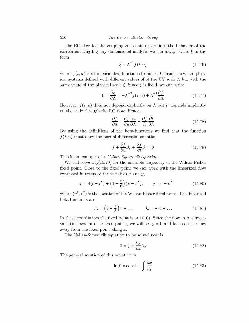
x
x1 x2 x
Figure 15.12 RG flows along the scaled variable x with two initial values,x1 and x2, and the same final value x.
Let us consider two flows along x with different starting points, x1 andx2, and with the same final point x, with the same UV cutoff Λ0 (shown inFig.15.12). The value of the correlation length ξ at x1 and x2 is
ξ(x1) = Λ−10 f(x1), ξ(x2) = Λ
−10 f(x2) (15.85)
where
f(x1) =f(x) exp (∫ x
x1
dx
β(x))f(x2) =f(x) exp (∫ x
x2
dx
β(x)) (15.86)
Hence, we find
ξ(x1) = ξ(x2) exp (∫ x2
x1
dx
β(x)) (15.87)
Suppose now that x1 is very close to the fixed point (x1 → 0) and that x2is far away enough that ξ(x1) ≃ a (the short distance cutoff). Using thelinearized beta-function, we find that
ξ(x1) ≃ a exp (∫ x2
x1
dx(2 − ϵ3)x) = a
!!!!!!x1x2 !!!!!!−ν
(15.88)
where
ν =1
β′(0) =1
2− ϵ3
=12+
ϵ
12+O(ϵ2) (15.89)
Hence, the value of the critical exponent ν of the correlation length is de-termined by the slope of the beta-function at the Wilson-Fisher fixed point,which at the present level of approximation is β′(0) = 2− ϵ
3+O(ϵ2).
518 The Renormalization Group
15.3 General properties of a fixed point theory
We see that at a fixed point of a renormalization group transformation thetheory has an emergent symmetry: scale-invariance. This emergent symme-try is operative at length scales long compared to a short-distance cutoff a
(the UV regulator) but short compared to the linear size L of the system(the IR regulator). No other scales are present at the fixed point. In Chap-ter 21 we will see that, in most cases of interest, in quantum field theoryscale invariance can be extended to a larger emergent symmetry, confor-mal invariance, i.e. invariance under conformal coordinate transformationsx′= f(x) such that angles between vectors are preserved. There we will
show that most of the statements that we will make in this section followfrom conformal invariance. In this section we will explore the consequencesof these assumptions for the properties of theories at a fixed point. The dis-cussion presented here follows two excellent sources: Paul Ginsparg’s 1988Les Houches Lectures (Ginsparg, 1989), and John Cardy’s book on scalingand renormalization (Cardy, 1996).
In a scale-invariant theory the action (or, more precisely, the partitionfunction) is invariant under scale transformations, x ↦ x
′= λx. In such a
theory, the expectation values of the observables transform under dilationsas homogenous functions. A function F (x) is a homogenous function ofdegree k if F (λx) = λ
kF (x).
From the scale invariance of the partition function it follows that at, ageneral fixed point whose action we will denote by S
∗, the correlators ofa physical local observable O(x) must be homogeneous functions of thedistance ∣x − y∣ and should obey power laws of the form
⟨O(x)O(y)⟩∗ =const.∣x − y∣2∆O
(15.90)
Here ⟨A⟩∗ denotes the expectation value of the observable A at the fixedpoint S∗. The quantity ∆O is called the scaling dimension of the local op-erator O. Hence, at the fixed point, the operator O has units of
[O] = ℓ−∆O (15.91)
where ℓ is a length scale.The scaling dimensions of the observables are one of the universal prop-
erties that define a fixed point. A universal quantity here means a quantitywhose value is independent of the short-distance definition of the theory,i.e. of its definition in the UV. Clearly, dimensionful quantities are by def-inition not universal since a microscopic scale is needed to define the units
15.3 General properties of a fixed point theory 519
and different choices will lead to different values. Hence, only dimensionlessquantities, such as the scaling dimensions, can be universal.
At a general fixed point, the scaling dimensions of the operators mustbe positive real numbers so that the correlators of local observables obeycluster decomposition, and must decay (as a power law in this case) at largeseparations. In exceptional cases, the scaling dimensions take rational values.This is the case in scale-invariant free field theories and also in integrablesystems such as the minimal models of D = 2 dimensional conformal fieldtheories that will be discussed in Chapter 21. There we will show that atheory with conformal invariance has the following properties:
1) The theory has a conformally-invariant vacuum state ∣0⟩.2) It has a set of operators, that we will denote by {φj}, called quasi-primary,
which transforms irreducibly under conformal transformations, meaningthat they obey the transformation law
φj(x) ↦ !!!!!!!!!∂x
′
∂x
!!!!!!!!!∆j/D
φj(x′) (15.92)
where
J =
!!!!!!!!!∂x
′
∂x
!!!!!!!!! (15.93)
is the Jacobian of the conformal transformation, D is the space-time di-mension, and the numbers {∆j} are the scaling-dimensions of the oper-ators. The scaling dimensions are the quantum numbers that label therepresentations of the conformal group.
3) Under a conformal transformation the correlators of the fields transformas
⟨φ1(x1) . . .φN(xN )⟩∗ =
!!!!!!!!!∂x
′
∂x
!!!!!!!!!∆1/Dx=x1
. . .!!!!!!!!!∂x
′
∂x
!!!!!!!!!∆N/Dx=xN
⟨φ1(x′1) . . .φN (x′N)⟩∗(15.94)
4) All other operators in the theory are linear combinations of the quasi-primary fields and of their derivatives.
The symmetries of the fixed point strongly constrain the behavior of thecorrelators. Translation and rotation (or Lorentz) invariance require that theN -point functions depend only on the pairwise distances, ∣x12∣ = ∣x1 − x2∣.Scale invariance then requires that they depend only on scale-invariant ra-tios, ∣x12∣/∣x34∣. In addition, conformal invariance requires that they dependonly on the cross ratios ∣x12∣∣x34∣/(∣x13∣∣x24∣).
520 The Renormalization Group
Translation, rotation and scale invariance restrict the form of the two-point functions, ⟨φ1(x1)φ2(x2)⟩∗, to have the form
⟨φ1(x1)φ2(x2)⟩∗ =C12∣x12∣∆1+∆2
(15.95)
However, in Chapter 21 we will show that conformal invariance further re-stricts the form of the two-point functions, requiring that C12 = 0 if∆1 ≠ ∆2.Hence
⟨φ1(x1)φ2(x2)⟩∗ =
⎧⎪⎪⎪⎪⎨⎪⎪⎪⎪⎩C12∣x12∣2∆ , ∆ = ∆1 = ∆2
0, ∆1 ≠ ∆2
(15.96)
Hence, primary fields with different scaling dimensions (i.e. in different repre-sentations) are “orthogonal” to each other. Clearly, by a suitable redefinitionof the operators we can always set the non-vanishing coefficient C12 = 1.
The form of the three-point functions is also completely determined bytranslation, rotation, scale and conformal invariance. In Chapter 21 we willshow that the three-point function has the form (Polyakov, 1974)
⟨φ1(x1)φ2(x2)φ3(x3)⟩∗ =C123∣x12∣∆12∣x23∣∆23∣x31∣∆31
(15.97)
where ∆ij = ∆i+∆j −∆k (with i, j, k = 1, 2, 3). Provided the primary fieldsare normalized so that the coefficient of the two point function is Cij = δij ,the coefficients Cijk of the three-point functions are universal numbers whichfurther characterize the fixed point. We will see that they play a key role.
These symmetries also restrict the form of the higher point functions butnot as completely. For instance, the four-point function must have the form
⟨φ1(x1)φ2(x2)φ3(x3)φ4(x4)⟩∗ = F (∣x12∣∣x34∣∣x13∣∣x24∣) ∏i<j
1
∣xij∣∆i+∆j−∆/3(15.98)
where ∆ = ∑4i=1∆i. The function F (z), where z = ∣x12∣∣x34∣/(∣x13∣∣x24∣)
is the cross ratio of the coordinates of the four operators, is a universalscaling function. Similar, but more complicated expressions, apply for thehigher-order N -point functions (with N > 4).
15.4 The operator product expansion
Let us consider an N -point function of a theory at a general fixed point⟨φ1(x1) . . .φN(xN)⟩∗. Let us now consider the case in which two of theoperators, say φ1(x1) and φ2(x2) approach each other and, hence, they
15.4 The operator product expansion 521
closer to each other than to the insertions of any of the other operators, i.e.a ≪ ∣x12∣ ≪ ∣xij∣, where i = 1, 2 and j = 3, . . . , N (but still farther apartthan the scale of the UV cutoff a). The form of the N -point functions in afixed point theory (c.f. Eq.(15.98)) tells us that the N point function willbe singular as the coordinates of any pair of fields approach each other, andthat, furthermore, the singularity is determined by the scaling dimensionsof the fields involved.
This property suggests that this behavior should be the same as if theproduct of these two fields is replaced by some suitable combination of allthe operators in the theory. Thus, inside expectation values, the productof fields can be replaced by an expansion involving all other fields. Theprecise statement is as follows. Given that the set of operators {φj}, andtheir descendants (involving derivatives) are a complete set, it follows thatthe product of two such fields, say φi(x) and φj(y), should be equivalent atshort distance to a suitable linear combination of the fields {φk} and theirdescendants (Kadanoff, 1969; Wilson, 1969; Polyakov, 1970), i.e.
limy→x
φi(x)φj(y) = limy→x
∑k
Cijk∣x − y∣∆i+∆j−∆kφk (x + y
2) (15.99)
This statement is the content of the Operator Product Expansion (OPE).Notice that this operator identity is a weak identity as it is only meant tohold inside an expectation value of the fixed point theory. Also notice thatthe only operators φk that will contribute to the singular behavior musthave scaling dimensions such that ∆k ≤ ∆i +∆j .
We will now see that the coefficients of the OPE are the same as thecoefficients of the three-point functions. To this effect let us consider thethree point function ⟨φi(x)φj(y)φl(z)⟩∗, and use the OPE of Eq.(15.99) towrite
limy→x
⟨φi(x)φj(y)φl(z)⟩∗ = limy→x
∑k
Cijk∣x − y∣∆i+∆j−∆k⟨φk (x + y
2)φl(z)⟩∗
(15.100)We can now use the expressions for the two-point functions of Eq.(15.96) tofind that
limy→x
⟨φi(x)φj(y)φl(z)⟩∗ =∑k
Cijk limy→x
1∣x − y∣∆i+∆j−∆k⟨φk (x + y
2)φl(z)⟩∗
=Cijl limy→x
1∣x − y∣∆i+∆j−∆l
1∣x − z∣2∆l(15.101)
Using the expression for the three-point functions, Eq.(15.97), we readily
522 The Renormalization Group
find that
Cijk = Cijk (15.102)
In other terms, the coefficients of the OPE are the same as the coefficientsof the three-point functions (for normalized operators).
These results is also interpreted as meaning that at a fixed point theoperators (or fields) as they approach each other they satisfy a fusion algebrawhich is conventionally denoted as
[φi] ⋅ [φj] = ∑k
Cijk[φk] (15.103)
Here we did not write down explicitly the possible multiplicities of thesefusion channels. We will see below that the fusion algebra encodes the prop-erties of the one-loop renormalization group beta functions in the neighbor-hood of the fixed point.
15.5 Simple examples of fixed points
We will now discuss several simple examples of fixed points in free fieldtheories.
15.5.1 Free massless scalar field
Let φ(x) be a free massless scalar field in D Euclidean dimensions. TheLagrangian is
L =12(∂µφ)2 (15.104)
From dimensional analysis and the condition that action be dimensionlesswe see that the Lagrangian has units of [L] = ℓ
−D. Hence the free field φ
has units of [φ] = ℓ−(D−2)/2. Thus, the scaling dimension of the free field
φ(x) is
∆φ =12(D − 2) (15.105)
which is consistent with the fact that the two-point function of a free scalarfield is
⟨φ(x)φ(y)⟩ = const.∣x − y∣2∆φ (15.106)
where 2∆φ = D − 2.
15.5 Simple examples of fixed points 523
In a free field it is trivial to find the scaling dimensions of all other oper-ators. Thus, the operator φn(x) has dimension
∆n ≡ ∆[φn] = n∆φ =n
2(D − 2) (15.107)
which is consistent with the two point function of the normal-ordered oper-ator ∶ φn(x) ∶,
⟨∶ φn(x) ∶∶ φn(y) ∶⟩ = const.∣x − y∣2∆n(15.108)
where here normal ordering means ∶ A ∶= A − ⟨A⟩. Another equivalent wayto see that Eq.(15.108) is correct is to use Wick’s theorem and show thatthe correlator of φn reduces to a sum of products of n two-point correlators.
These results are also consisten with a simple dimensional analysis of theLagrangian. Indeed, under a scale transformation x ↦ λx the scalar fieldtransforms as φ(λx) ↦ λ
−∆φφ(x), where ∆φ =12(D − 2), which leaves the
action invariant.
15.5.2 Free massless Dirac field
The Lagrangian of a free massless Dirac field in D dimensions is
L = ψ(x)iγµ∂µψ(x) (15.109)
where ψ(x) is a spinor Fermi field, with two components in D = 2, 3 dimen-sions, four components in D = 4, 5 dimensions, etc, and γµ are the Diracmatrices in D dimensions.
By dimensional analysis, we see that the Dirac field has units of [ψ] =
ℓ−(D−1)/2. Hence, its scaling dimension is ∆ψ =
12(D−1), and the two-point
function is
⟨ψ(x)ψ(y)⟩ = const.∣x − y∣2∆ψ (15.110)
Similarly, the scaling dimension of a composite operator (ψψ)n is
∆((ψψ)n) = 2n∆ψ = n(D − 1) (15.111)
In particular, the current operator jµ = ψγµψ has scaling dimension D − 1.
15.5.3 Gauge theories
The Lagrangian for a gauge theory is
L =1
4g2trF
2µν (15.112)
524 The Renormalization Group
where the field strength is Fµν = i[Dµ,Dν] = ∂µAν − ∂νAµ + [Aµ, Aν], andDµ = ∂µ+ iAµ is the covariant derivative. From the fact that the gauge field
is a one-form it follows that it has units of [A] = ℓ−1, and hence its scaling
dimension is ∆[A] = 1. Notice that here the coupling constant is in theprefactor of the Lagrangian. Thus the field strength has scaling dimension∆[F ] = 2. The action is dimensionaless if we assign the coupling constantunits of [g] = (D − 4)/2.
15.6 Perturbing a fixed point theory
We will now consider a theory close to a fixed point. We will use perturba-tion theory in powers of the coupling constants of the theory. We will usethis framework to derive the general form of the renormalization group betafunctions close to a general fixed point theory. This approach is known asconformal perturbation theory. It is a generalization of the Kosterlitz renor-malization group (Kosterlitz, 1974) used to describe the Kosterlitz-Thoulessphase transition in two-dimensional Classical Statistical Mechanics (Koster-litz and Thouless, 1973). An insightful discussion of this renormalizationgroup is presented in Cardy’s book (Cardy, 1996), whose approach we willfollow closely.
Let S∗ be the action of a fixed point theory in D Euclidean dimensions.Let δS be a set of general perturbations parametrized by the complete setof primary fields {φj} of the fixed point. The total action S is
S = S∗+ δS = S
∗+∑
j
∫ dxDgj a
∆j−Dφj(x) (15.113)
where {gj} are the dimensionless coupling constants, the short distance scalea is the UV regulator, and {∆j} are the scaling dimensions of the fields {φj}.
Let Z be the path integral for this theory which we will formally denoteby
Z =tr exp(−S∗− δS)
=tr exp⎛⎜⎝−S∗
−∑j
∫ dDx gj a
∆j−Dφj(x)⎞⎟⎠=Z
∗× ⟨exp ⎛⎜⎝−∑
j
∫ dDx gj a
∆j−Dφj(x)⎞⎟⎠⟩∗
(15.114)
where Z∗= tr exp(−S∗) is the partition function of the fixed point theory.
15.6 Perturbing a fixed point theory 525
Here, as before, we represented expectation values in the fixed point theoryby the notation
⟨A⟩∗ =1
Z∗ tr (A exp(−S∗)) (15.115)
Our next step is to write the expansion of the partition function Z inpowers of the coupling constants {gj}:Z
Z∗ = ⟨exp ⎛⎜⎝−∑j
∫ dDx gj a
∆j−Dφj(x)⎞⎟⎠⟩∗
= 1−∑j
∫ dDx gj a
∆j−D⟨φj(x)⟩∗ (15.116)
+12!
∑j,k
∫ dDxj ∫ d
Dxk gjgk a
∆j+∆k−2D⟨φj(xj)φk(xk)⟩∗ (15.117)
−13!
∑j,k,l
∫ dDxj ∫ d
Dxk ∫ d
Dxl gjgkgl a
∆j+∆k+∆l−3D⟨φj(xj)φk(xk)φl(xl)⟩∗(15.118)
+ . . .
At a formal level, we can reinterpret this expression as the partition functionof a gas of particles of different types in a Grand Canonical Ensemble, witheach species labeled by j at coordinates xj. In this perspective, the couplingconstants gj play the role of the the fugacity of each type of particle and theinteractions are given by the (negative of) the logarithm of the correlatorsat the fixed point. Since S∗ is a fixed point action, the integrals of the corre-lators present in Eqs.(15.116), (15.117) and (15.118) will generally containIR divergencies. We will assume that the theory is in a box of linear size L
to cutoff the IR behavior. But, precisely because S∗ is a fixed point action
and hence is scale invariant, we will need essentially their short distance UVsingular behavior which is controlled by the OPE. We will control the short-distance singularities by cutting off the integrals at some short distance a.Hence, the span of the integrals will be the range L ≫ ∣xj − xk∣ ≫ a. Inother words, the “particles” of this gas have a “hard-core” a.
We will analyze this expansion using the following renormalization grouptransformation. We will attempt to change the UV cutoff a by some smallamount δa = aδℓ (with δℓ ≪ 1) and then compute the change of the actionneeded to compensate for that change, while requiring that the full partitionfunction Z be left unchanged in a box of fixed linear size L. Instead ofintegrating out modes in momentum-shells, as we did in Section 15.2.4, here
526 The Renormalization Group
we will integrate out contributions to the integrals appearing in Eqs.(15.116),(15.117) and (15.118) in a shell in real space comprised between the UVcutoff a and the dilated cutoff ba, with b = 1 + δℓ. We will proceed asfollows:
We rescale the UV cutoff a ↦ ba, with b = 1 + δℓ > 1. Hence, we areincreasing the UV cutoff. We will then need to rescale the coupling constants{gj} to compensate for this change, while keeping Z unchanged. How do wedo this? The UV cutoff a appears in three places
a) in factors of the form a∆j−D, where ∆j is the scaling dimension of the
operators,
b) as a UV cutoff of the integrals,
c) through the dependence of the integrals on the IR cutoff L, which by scaleinvariance must enter in the form L/a.
If the relative change of UV scale is small, i.e. δℓ ≪ 1, we will need to lookonly for linear changes in δℓ. Since these factors always appear multiplyingthe dimensionless coupling constants gj ,
gja∆j−D ↦ gja
∆j−Db∆j−D (15.119)
we can compensate this change by a change in the coupling constants,
gj ↦ gjbD−∆j
= gj(i + (D −∆j)δℓ) (15.120)
Hence, we will change the coupling constants by
gj ↦ gj + (D −∆j)gjδℓ (15.121)
Next, we compute the result of a change the cutoff in the integrals. Thisamounts to computing the contributions to the integrals in the shell in realspace a(1+δℓ) > ∣xi−xj∣ > a (instead of a shell in momentum space). Thuswe split the integrals as follows
∫∣xi−xj∣>a(1+δℓ) = ∫∣xi−xj∣>a−∫a(1+δℓ)>∣xi−xj∣>a (15.122)
The application of this analysis to the terms linear in the coupling constants,Eq.(15.116), yields a purely numerical contribution to the partition functionZ (and hence it amounts to a renormalization of the identity operator). Thecontribution of the terms quadric in the coupling constants, Eq.(15.117),can be computed using the OPE. This is legitimate since we will look atcontributions only inside the infinitesimal shell in real space. Using the OPE
15.7 Example of OPEs: φ4 theory 527
we find that this contribution is
12!
∑j,k
∑l
Cjkl gjgk a∆l−∆j−∆k ∫
shelldDxjd
Dxk⟨φl((xj + xk)/2)⟩∗a∆j+∆k−2D
=12!
∑j,k
∑l
Cjkl gjgk a∆l−D ∫ d
Dx⟨φl(x)⟩∗SDδℓ (15.123)
where
SD =2πD
Γ(D/2) (15.124)
is the area of the hypersphere in D dimensions and Γ(x) is the Euler Gammafunction. The “one-loop” contribution, Eq.(15.123), can be compensated bya change in the coupling constants
gl ↦ gl −12SD ∑
j,k
gjgkCjklδℓ (15.125)
In fact, the structure of the OPEs implies that similar changes happen atall orders in the expansion.
Finally, there is the dependence in a due to the dependence in L. However,in order to keep the system unchanged the IR cutoff L must be held fixed.Hence this dependence is trivial.
We now collect all the changes in the coupling constants in the differentialequation
dgldℓ
= (D −∆l)gl −∑j,k
Cjklgjgk + . . . (15.126)
where we absorbed a factor of SD/2 in a (multiplicative) redefinition of thecoupling constants. In summary, we derived the beta-functions for all thecoupling constants using conformal perturbation theory to order one-loop.As we can see, the beta functions depend on the data of the fixed point: thescaling dimensions ∆j , and the coefficients Cijk of the OPEs of the primaryfields. This a general result for all fixed point theories.
15.7 Example of OPEs: φ4theory
We will now apply the ideas of the preceding sections to the free field fixedpoint of φ4 theory. The Euclidean Lagrangian is
L =12(∂µφ)2 + ta
−2φ2+ ua
D−4φ4+ ha
−(1+D/2)φ (15.127)
528 The Renormalization Group
where we defined the mass m2, the coupling constant λ, and the symmetrybreaking field J in terms the dimensionless couplings, t, u and h,
m2= ta
−2, λ = ua
D−4, J = ha
−(1+D/2)(15.128)
Let us now define the normal ordered composite operators
∶ φ2∶= φ
2− ⟨φ2⟩, ∶ φ
4∶= φ
4− 3⟨φ2⟩φ2, etc (15.129)
In what follows we will use the notations φn =∶ φn∶. Clearly, φ1 = φ since⟨φ⟩∗ = 0 at the free field fixed point.
Let us begin by computing the OPE of two φ ≡ φ1 fields. Using our resultswe find
limy→x
φ1(x)φ1(y) = limy→x
∶ φ(x) ∶∶ φ(y) ∶= lim
y→x[ 1∣x − y∣D−2
+ ∶ φ2 ((x + y)/2) ∶ + . . .] (15.130)
Notice that the first term, proportional to the identity operator, is the mostsingular term in the expansion, and that the next term is finite (as ∣x−y∣ →0). The next possible operator would be ∶ (∂φ)2 ∶. However, its coefficientwill vanish as ∣x − y∣2. Hence, in the limit it does not contribute. Onlysingular and finite terms will be kept in the expansion.
We will record this equation as the OPE of two φ1 fields
[φ1] ⋅ [φ1] = [1] + [φ2] (15.131)
where 1 denotes the identity field.Next we compute the OPE of a φ1 field (i.e. the field φ itself) and the
φ2 ≡∶ φ(x)2 ∶ field. Using Wick’s theorem we find
[φ1] ⋅ [φ2] = 2[φ1] + [φ3] (15.132)
where φ3 =∶ φ(x)3 ∶.Next we compute the OPE of two φ2 =∶ φ
2∶ fields. Again, using Wick’s
theorem, we obtain
limy→x
∶ φ2(x) ∶∶ φ2(y) ∶= lim
y→x[ 2∣x − y∣2(D−2) +
4∣x − y]D−2∶ φ
2((x + y)/2) ∶ + . . .](15.133)
which we will record as
[φ2] ⋅ [φ2] = 2+ 4[φ2]+ [φ4] (15.134)
15.7 Example of OPEs: φ4 theory 529
The following OPEs are derived in a similar fashion
[φ1] ⋅ [φ4] =4[φ3] (15.135)[φ2] ⋅ [φ4] =12[φ2] + 8[φ4] (15.136)[φ4] ⋅ [φ4] =24 + 96[φ2] + 72[φ4] (15.137)
Notice that we have neglected possible descendant operators, such as∶ (∂µφ)2 ∶, ∶ (∂2φ)2 ∶, ∶ (∂µφ)4 ∶, etc. These higher derivative operatorsare typically leading irrelevant operators. This is however not always thecase. For instance in the OPE of ∶ φ2 ∶ with itself the operator ∶ (∂µφ)2 ∶
can appear. By matching scaling dimensions we see that the prefactor of∶ (∂µφ)2 ∶ must be proportional to ∣x − y∣−(D−4), which is singular if D > 4and has a logarithmic divergence if D = 4. These contributions, however,enter in higher order loops (as we will see in Chapter 16).
Using these results we can now write the beta functions for φ4 theory.With the identification g1 = h (the symmetry breaking field), g2 = t (thedimensionless mass squared), and g4 = u (the coupling constant), we findthat their one-loop beta functions are
dh
dℓ= (D
2+ 1)h− 4ht + . . . (15.138)
dt
dℓ=2t − 4h
2− 4t
2− 24tu − 96u
2+ . . . (15.139)
du
dℓ=(4 −D)u − t
2− 16tu − 72u
2+ . . . (15.140)
For D = 4 − ϵ, these beta functions have two fixed points: a) the trivialfixed point at h∗ = t
∗= u
∗= 0, and b) the non-trivial Wilson-Fisher fixed
point at h∗= 0, t∗ = O(ϵ2), and u
∗=
ϵ72
+ O(ϵ2). The critical exponent νof the correlation length is the inverse of the slope of the beta function for tat the Wilson-Fisher fixed point. We obtain, ν =
12+ ϵ
12+O(ϵ2), consistent
with what we found before. Also notice that since t∗ = O(ϵ2), the anomalousdimension of the field φ is zero at one-loop order. We will see in Chapter 16that it is non-zero at two-loop order.