14.NEUTRINOMASS,MIXING,ANDOSCILLATIONSpdg.lbl.gov/2016/reviews/rpp2016-rev-neutrino-mixing.pdf ·...
85
14. Neutrino mixing 1 14. NEUTRINO MASS, MIXING, AND OSCILLATIONS Updated June 2016 by K. Nakamura (Kavli IPMU (WPI), U. Tokyo, KEK), and S.T. Petcov (SISSA/INFN Trieste, Kavli IPMU (WPI), U. Tokyo, Bulgarian Academy of Sciences). The experiments with solar, atmospheric, reactor and accelerator neutrinos have provided compelling evidences for oscillations of neutrinos caused by nonzero neutrino masses and neutrino mixing. The data imply the existence of 3-neutrino mixing in vacuum. We review the theory of neutrino oscillations, the phenomenology of neutrino mixing, the problem of the nature - Dirac or Majorana, of massive neutrinos, the issue of CP violation in the lepton sector, and the current data on the neutrino masses and mixing parameters. The open questions and the main goals of future research in the field of neutrino mixing and oscillations are outlined. 14.1. Introduction: Massive neutrinos and neutrino mixing It is a well-established experimental fact that the neutrinos and antineutrinos which take part in the standard charged current (CC) and neutral current (NC) weak interaction are of three varieties (types) or flavours: electron, ν e and ¯ ν e , muon, ν μ and ¯ ν μ , and tauon, ν τ and ¯ ν τ . The notion of neutrino type or flavour is dynamical: ν e is the neutrino which is produced with e + , or produces an e − , in CC weak interaction processes; ν μ is the neutrino which is produced with μ + , or produces μ − , etc. The flavour of a given neutrino is Lorentz invariant. Among the three different flavour neutrinos and antineutrinos, no two are identical. Correspondingly, the states which describe different flavour neutrinos must be orthogonal (within the precision of the current data): 〈ν l ′ |ν l 〉 = δ l ′ l , 〈 ¯ ν l ′ | ¯ ν l 〉 = δ l ′ l , 〈 ¯ ν l ′ |ν l 〉 = 0. It is also well-known from the existing data (all neutrino experiments were done so far with relativistic neutrinos or antineutrinos), that the flavour neutrinos ν l (antineutrinos ¯ ν l ), are always produced in weak interaction processes in a state that is predominantly left-handed (LH) (right-handed (RH)). To account for this fact, ν l and ¯ ν l are described in the Standard Model (SM) by a chiral LH flavour neutrino field ν lL (x), l = e, μ, τ . For massless ν l , the state of ν l (¯ ν l ) which the field ν lL (x) annihilates (creates) is with helicity (-1/2) (helicity +1/2). If ν l has a non-zero mass m(ν l ), the state of ν l (¯ ν l ) is a linear superposition of the helicity (-1/2) and (+1/2) states, but the helicity +1/2 state (helicity (-1/2) state) enters into the superposition with a coefficient ∝ m(ν l )/E , E being the neutrino energy, and thus is strongly suppressed. Together with the LH charged lepton field l L (x), ν lL (x) forms an SU (2) L doublet. In the absence of neutrino mixing and zero neutrino masses, ν lL (x) and l L (x) can be assigned one unit of the additive lepton charge L l and the three charges L l , l = e, μ, τ , are conserved by the weak interaction. C. Patrignani et al. (Particle Data Group), Chin. Phys. C, 40, 100001 (2016) October 6, 2016 11:02
-
Upload
nguyenminh -
Category
Documents
-
view
216 -
download
0
Transcript of 14.NEUTRINOMASS,MIXING,ANDOSCILLATIONSpdg.lbl.gov/2016/reviews/rpp2016-rev-neutrino-mixing.pdf ·...
14. Neutrino mixing 1
14. NEUTRINO MASS, MIXING, AND OSCILLATIONS
Updated June 2016 by K. Nakamura (Kavli IPMU (WPI), U. Tokyo, KEK), andS.T. Petcov (SISSA/INFN Trieste, Kavli IPMU (WPI), U. Tokyo, Bulgarian Academy ofSciences).
The experiments with solar, atmospheric, reactor and accelerator neutrinos haveprovided compelling evidences for oscillations of neutrinos caused by nonzero neutrinomasses and neutrino mixing. The data imply the existence of 3-neutrino mixing invacuum. We review the theory of neutrino oscillations, the phenomenology of neutrinomixing, the problem of the nature - Dirac or Majorana, of massive neutrinos, the issueof CP violation in the lepton sector, and the current data on the neutrino masses andmixing parameters. The open questions and the main goals of future research in the fieldof neutrino mixing and oscillations are outlined.
14.1. Introduction: Massive neutrinos and neutrino mixing
It is a well-established experimental fact that the neutrinos and antineutrinos whichtake part in the standard charged current (CC) and neutral current (NC) weak interactionare of three varieties (types) or flavours: electron, νe and νe, muon, νµ and νµ, and tauon,ντ and ντ . The notion of neutrino type or flavour is dynamical: νe is the neutrino whichis produced with e+, or produces an e−, in CC weak interaction processes; νµ is theneutrino which is produced with µ+, or produces µ−, etc. The flavour of a given neutrinois Lorentz invariant. Among the three different flavour neutrinos and antineutrinos, notwo are identical. Correspondingly, the states which describe different flavour neutrinosmust be orthogonal (within the precision of the current data): 〈νl′ |νl〉 = δl′l, 〈νl′ |νl〉 = δl′l,〈νl′ |νl〉 = 0.
It is also well-known from the existing data (all neutrino experiments were done so farwith relativistic neutrinos or antineutrinos), that the flavour neutrinos νl (antineutrinosνl), are always produced in weak interaction processes in a state that is predominantlyleft-handed (LH) (right-handed (RH)). To account for this fact, νl and νl are describedin the Standard Model (SM) by a chiral LH flavour neutrino field νlL(x), l = e, µ, τ . Formassless νl, the state of νl (νl) which the field νlL(x) annihilates (creates) is with helicity(-1/2) (helicity +1/2). If νl has a non-zero mass m(νl), the state of νl (νl) is a linearsuperposition of the helicity (-1/2) and (+1/2) states, but the helicity +1/2 state (helicity(-1/2) state) enters into the superposition with a coefficient ∝ m(νl)/E, E being theneutrino energy, and thus is strongly suppressed. Together with the LH charged leptonfield lL(x), νlL(x) forms an SU(2)L doublet. In the absence of neutrino mixing and zeroneutrino masses, νlL(x) and lL(x) can be assigned one unit of the additive lepton chargeLl and the three charges Ll, l = e, µ, τ , are conserved by the weak interaction.
C. Patrignani et al. (Particle Data Group), Chin. Phys. C, 40, 100001 (2016)October 6, 2016 11:02
2 14. Neutrino mixing
At present there is no compelling evidence for the existence of states of relativisticneutrinos (antineutrinos), which are predominantly right-handed, νR (left-handed, νL).If RH neutrinos and LH antineutrinos exist, their interaction with matter should be muchweaker than the weak interaction of the flavour LH neutrinos νl and RH antineutrinosνl, i.e., νR (νL) should be “sterile” or “inert” neutrinos (antineutrinos) [1]. In theformalism of the Standard Model, the sterile νR and νL can be described by SU(2)Lsinglet RH neutrino fields νR(x). In this case, νR and νL will have no gauge interactions,i.e., will not couple to the weak W± and Z0 bosons. If present in an extension ofthe Standard Model, the RH neutrinos can play a crucial role i) in the generation ofneutrino masses and mixing, ii) in understanding the remarkable disparity between themagnitudes of neutrino masses and the masses of the charged leptons and quarks, and iii)in the generation of the observed matter-antimatter asymmetry of the Universe (via theleptogenesis mechanism [2]) . In this scenario which is based on the see-saw theory [3],there is a link between the generation of neutrino masses and the generation of the baryonasymmetry of the Universe. The simplest hypothesis (based on symmetry considerations)is that to each LH flavour neutrino field νlL(x) there corresponds a RH neutrino fieldνlR(x), l = e, µ, τ , although schemes with less (more) than three RH neutrinos are alsobeing considered.
The experiments with solar, atmospheric, reactor and accelerator neutrinos haveprovided compelling evidences for the existence of neutrino oscillations [4,5], transitionsin flight between the different flavour neutrinos νe, νµ, ντ (antineutrinos νe, νµ, ντ ),caused by nonzero neutrino masses and neutrino mixing. The existence of flavour neutrinooscillations implies that if a neutrino of a given flavour, say νµ, with energy E is producedin some weak interaction process, at a sufficiently large distance L from the νµ source theprobability to find a neutrino of a different flavour, say ντ , P (νµ → ντ ; E, L), is differentfrom zero. P (νµ → ντ ; E, L) is called the νµ → ντ oscillation or transition probability.If P (νµ → ντ ; E, L) 6= 0, the probability that νµ will not change into a neutrino of adifferent flavour, i.e., the “νµ survival probability” P (νµ → νµ; E, L), will be smaller thanone. If only muon neutrinos νµ are detected in a given experiment and they take part inoscillations, one would observe a “disappearance” of muon neutrinos on the way from theνµ source to the detector. Disappearance of the solar νe, reactor νe and of atmospheric νµ
and νµ due to the oscillations have been observed respectively, in the solar neutrino [6–14],KamLAND [15,16] and Super-Kamokande [17,18] experiments. Strong evidences for νµ
disappearance due to oscillations were obtained also in the long-baseline acceleratorneutrino experiments K2K [19]. Subsequently, the MINOS [20,21] and T2K [22,23]long baseline experiments reported compelling evidence for νµ disappearance due tooscillations, while evidences for ντ appearance due to νµ → ντ oscillations were publishedby the Super-Kamiokande [24] and OPERA [25] collaborations. As a consequence of theresults of the experiments quoted above the existence of oscillations or transitions of thesolar νe, atmospheric νµ and νµ, accelerator νµ (at L ∼ 250 km, L ∼ 295 km and L ∼ 730km) and reactor νe (at L ∼ 180 km), driven by nonzero neutrino masses and neutrinomixing, was firmly established. There are strong indications that the solar νe transitionsare affected by the solar matter [26,27].
Further important developments took place in the period starting from June 2011.
October 6, 2016 11:02
14. Neutrino mixing 3
First, the T2K Collaboration reported [28] indications for νµ → νe oscillations, i.e.,of “appearance” of νe in a beam of νµ, which had a statistical significance of 2.5σ.The MINOS [29] Collaboration also obtained data consistent with νµ → νe oscillations.Subsequently, the Double Chooz Collaboration reported [30] indications for disappearanceof reactor νe at L ∼ 1.1 km. Strong evidences for reactor νe disappearance at L ∼ 1.65km and L ∼ 1.38 km and (with statistical significance of 5.2σ and 4.9σ) were obtainedrespectively in the Daya Bay [31] and RENO [32] experiments. Further evidences forreactor νe disappearance (at 2.9σ) and for νµ → νe oscillations (at 3.1σ) were reportedby the Double Chooz [33] and T2K [34] experiments, while the Daya Bay and RENOCollaborations presented updated, more precise results on reactor νe disappearance[35,36,37]( for the latest results of the Daya Bay [38], RENO [39], Double Chooz [40],MINOS [41] and T2K experiments [42], see Section 14.12).
Oscillations of neutrinos are a consequence of the presence of flavour neutrino mixing,or lepton mixing, in vacuum. In the formalism of local quantum field theory, used toconstruct the Standard Model, this means that the LH flavour neutrino fields νlL(x),which enter into the expression for the lepton current in the CC weak interactionLagrangian, are linear combinations of the fields of three (or more) neutrinos νj , havingmasses mj 6= 0:
νlL(x) =∑
j
Ulj νjL(x), l = e, µ, τ, (14.1)
where νjL(x) is the LH component of the field of νj possessing a mass mj and U is aunitary matrix - the neutrino mixing matrix [1,4,5]. The matrix U is often called thePontecorvo-Maki-Nakagawa-Sakata (PMNS) or Maki-Nakagawa-Sakata (MNS) mixingmatrix. Obviously, Eq. (14.1) implies that the individual lepton charges Ll, l = e, µ, τ ,are not conserved.
All compelling neutrino oscillation data can be described assuming 3-flavour neutrinomixing in vacuum. The data on the invisible decay width of the Z-boson is compatiblewith only 3 light flavour neutrinos coupled to Z [43]. The number of massive neutrinosνj , n, can, in general, be bigger than 3, n > 3, if, for instance, there exist sterile neutrinosand they mix with the flavour neutrinos. It is firmly established on the basis of thecurrent data that at least 3 of the neutrinos νj , say ν1, ν2, ν3, must be light, m1,2,3 . 1eV (Section 14.12), and must have different masses, m1 6= m2 6= m3. At present thereare several experimental hints for existence of one or two light sterile neutrinos at the eVscale, which mix with the flavour neutrinos, implying the presence in the neutrino mixingof additional one or two neutrinos, ν4 or ν4,5, with masses m4 (m4,5) ∼ 1 eV. Thesehints will be briefly discussed in Section 14.13 of the present review.
Being electrically neutral, the neutrinos with definite mass νj can be Dirac fermionsor Majorana particles [44,45]. The first possibility is realized when there exists a leptoncharge carried by the neutrinos νj , which is conserved by the particle interactions. Thiscould be, e.g., the total lepton charge L = Le + Lµ + Lτ : L(νj) = 1, j = 1, 2, 3. In thiscase the neutrino νj has a distinctive antiparticle νj : νj differs from νj by the value ofthe lepton charge L it carries, L(νj) = − 1. The massive neutrinos νj can be Majoranaparticles if no lepton charge is conserved (see, e.g., Refs. [46,47]) . A massive Majorana
October 6, 2016 11:02
4 14. Neutrino mixing
particle χj is identical with its antiparticle χj : χj ≡ χj . On the basis of the existingneutrino data it is impossible to determine whether the massive neutrinos are Dirac orMajorana fermions.
In the case of n neutrino flavours and n massive neutrinos, the n × n unitary neutrinomixing matrix U can be parametrized by n(n − 1)/2 Euler angles and n(n + 1)/2 phases.If the massive neutrinos νj are Dirac particles, only (n − 1)(n − 2)/2 phases are physicaland can be responsible for CP violation in the lepton sector. In this respect the neutrino(lepton) mixing with Dirac massive neutrinos is similar to the quark mixing. For n = 3there is just one CP violating phase in U , which is usually called “the Dirac CP violatingphase.” CP invariance holds if (in a certain standard convention) U is real, U∗ = U .
If, however, the massive neutrinos are Majorana fermions, νj ≡ χj , the neutrinomixing matrix U contains n(n − 1)/2 CP violation phases [48,49], i.e., by (n − 1) phasesmore than in the Dirac neutrino case: in contrast to Dirac fields, the massive Majorananeutrino fields cannot “absorb” phases. In this case U can be cast in the form [48]
U = V P (14.2)
where the matrix V contains the (n − 1)(n − 2)/2 Dirac CP violation phases, while P isa diagonal matrix with the additional (n − 1) Majorana CP violation phases α21, α31,...,αn1,
P = diag(
1, eiα212 , ei
α312 , ..., ei
αn12
)
. (14.3)
The Majorana phases will conserve CP if [50] αj1 = πqj , qj = 0, 1, 2, j = 2, 3, ..., n. Inthis case exp[i(αj1 − αk1)] = ±1 has a simple physical interpretation: this is the relativeCP-parity of Majorana neutrinos χj and χk. The condition of CP invariance of theleptonic CC weak interaction in the case of mixing and massive Majorana neutrinosreads [46]:
U∗lj = Ulj ρj , ρj =
1
iηCP (χj) = ±1 , (14.4)
where ηCP (χj) = iρj = ±i is the CP parity of the Majorana neutrino χj [50]. Thus, ifCP invariance holds, the elements of U are either real or purely imaginary.
In the case of n = 3 there are altogether 3 CP violation phases - one Dirac andtwo Majorana. Even in the mixing involving only 2 massive Majorana neutrinos thereis one physical CP violation Majorana phase. In contrast, the CC weak interaction isautomatically CP-invariant in the case of mixing of two massive Dirac neutrinos or of twoquarks.
October 6, 2016 11:02
14. Neutrino mixing 5
14.2. The three neutrino mixing
All existing compelling data on neutrino oscillations can be described assuming3-flavour neutrino mixing in vacuum. This is the minimal neutrino mixing schemewhich can account for the currently available data on the oscillations of the solar (νe),atmospheric (νµ and νµ), reactor (νe) and accelerator (νµ and νµ) neutrinos. The(left-handed) fields of the flavour neutrinos νe, νµ and ντ in the expression for the weakcharged lepton current in the CC weak interaction Lagrangian, are linear combinations ofthe LH components of the fields of three massive neutrinos νj :
LCC = − g√2
∑
l=e,µ,τ
lL(x) γα νlL(x) Wα†(x) + h.c. ,
νlL(x) =
3∑
j=1
Ulj νjL(x), (14.5)
where U is the 3 × 3 unitary neutrino mixing matrix [4,5]. As we have discussed in thepreceding Section, the mixing matrix U can be parameterized by 3 angles, and, dependingon whether the massive neutrinos νj are Dirac or Majorana particles, by 1 or 3 CPviolation phases [48,49]:
U =
c12c13 s12c13 s13e−iδ
−s12c23 − c12s23s13eiδ c12c23 − s12s23s13e
iδ s23c13s12s23 − c12c23s13e
iδ −c12s23 − s12c23s13eiδ c23c13
× diag(1, eiα212 , ei
α312 ) . (14.6)
where cij = cos θij , sij = sin θij , the angles θij = [0, π/2], δ = [0, 2π] is the Dirac CPviolation phase and α21, α31 are two Majorana CP violation (CPV) phases. Thus, in thecase of massive Dirac neutrinos, the neutrino mixing matrix U is similar, in what concernsthe number of mixing angles and CPV phases, to the CKM quark mixing matrix. Thepresence of two additional physical CPV phases in U if νj are Majorana particles is aconsequence of the special properties of the latter (see, e.g., Refs. [46,48]) .
As we see, the fundamental parameters characterizing the 3-neutrino mixing are: i)the 3 angles θ12, θ23, θ13, ii) depending on the nature of massive neutrinos νj - 1 Dirac(δ), or 1 Dirac + 2 Majorana (δ, α21, α31), CPV phases, and iii) the 3 neutrino masses,m1, m2, m3. Thus, depending on whether the massive neutrinos are Dirac or Majoranaparticles, this makes 7 or 9 additional parameters in the minimally extended StandardModel of particle interactions with massive neutrinos.
The angles θ12, θ23 and θ13 can be defined via the elements of the neutrino mixingmatrix:
c212 ≡ cos2 θ12 =|Ue1|2
1 − |Ue3|2, s2
12 ≡ sin2 θ12 =|Ue2|2
1 − |Ue3|2, (14.7)
s213 ≡ sin2 θ13 = |Ue3|2, s2
23 ≡ sin2 θ23 =|Uµ3|2
1 − |Ue3|2,
c223 ≡ cos2 θ23 =|Uτ3|2
1 − |Ue3|2. (14.8)
October 6, 2016 11:02
6 14. Neutrino mixing
The neutrino oscillation probabilities depend (Section 14.7), in general, on the neutrinoenergy, E, the source-detector distance L, on the elements of U and, for relativisticneutrinos used in all neutrino experiments performed so far, on ∆m2
ij ≡ (m2i − m2
j ),i 6= j. In the case of 3-neutrino mixing there are only two independent neutrino masssquared differences, say ∆m2
21 6= 0 and ∆m231 6= 0. The numbering of massive neutrinos
νj is arbitrary. It proves convenient from the point of view of relating the mixing angles
θ12, θ23 and θ13 to observables, to identify |∆m221| with the smaller of the two neutrino
mass squared differences, which, as it follows from the data, is responsible for the solarνe and, the observed by KamLAND, reactor νe oscillations. We will number (just forconvenience) the massive neutrinos in such a way that m1 < m2, so that ∆m2
21 > 0. Withthese choices made, there are two possibilities: either m1 < m2 < m3, or m3 < m1 < m2.Then the larger neutrino mass square difference |∆m2
31| or |∆m232|, can be associated with
the experimentally observed oscillations of the atmospheric and accelerator νµ and νµ, aswell as of the reactor νe at L ∼ 1 km. The effects of ∆m2
31 or ∆m232 in the oscillations of
solar νe, and of ∆m221 in the oscillations of atmospheric and accelerator νµ and νµ or of
the reactor νe at L ∼ 1 km, are relatively small and subdominant as a consequence of thefacts that i) L, E and L/E in the experiments with solar νe and with atmospheric andaccelerator νµ and νµ, or with reactor νe and baseline L ∼ 1 km, are very different, ii)the conditions of production and propagation (on the way to the detector) of the solar νe
and of the atmospheric or accelerator νµ and νµ and of the reactor νe, are very different,and iii) |∆m2
21| and |∆m231| (|∆m2
32|) in the case of m1 < m2 < m3 (m3 < m1 < m2), asit follows from the data, differ by approximately a factor of 30, |∆m2
21| ≪ |∆m231(32)|,
|∆m221|/|∆m2
31(32)| ∼= 0.03. This implies that in both cases of m1 < m2 < m3 and
m3 < m1 < m2 we have ∆m232
∼= ∆m231 with |∆m2
31 − ∆m232| = |∆m2
21| ≪ |∆m231,32|.
Obviously, in the case of m1 < m2 < m3 (m3 < m1 < m2) we have ∆m231(32) > 0
(∆m231(32) < 0).
It followed from the results of the Chooz experiment [51] with reactor νe and fromthe more recent data of the Daya Bay, RENO, Double Chooz and T2K experiments(which will be discussed in Section14.12), that, in the convention we use, in which0 < ∆m2
21 < |∆m231(32)|, the element |Ue3|=sin θ13 of the neutrino mixing matrix U
is relatively small. This makes it possible to identify the angles θ12 and θ23 as theneutrino mixing angles associated with the solar νe and the dominant atmospheric νµ
(and νµ) oscillations, respectively. The angles θ12 and θ23 are sometimes called “solar”and “atmospheric” neutrino mixing angles, and are sometimes denoted as θ12 = θ⊙ andθ23 = θA (or θatm), while ∆m2
21 and ∆m231 are often referred to as the “solar” and
“atmospheric” neutrino mass squared differences and are often denoted as ∆m221 ≡ ∆m2
⊙,
∆m231 ≡ ∆m2
A (or ∆m2atm).
The solar neutrino data tell us that ∆m221 cos 2θ12 > 0. In the convention employed by
us we have ∆m221 > 0. Correspondingly, in this convention one must have cos 2θ12 > 0.
Global analyses of the neutrino oscillation data [52,53,54] available by the second halfof 2014 allowed us to determine the 3-neutrino oscillation parameters ∆m2
21, θ12, |∆m231|
(|∆m232|), θ23 and θ13 with a relatively high precision.
October 6, 2016 11:02
14. Neutrino mixing 7
The authors of the three independent analyses [52,53,54] report practically the same(within 1σ) results on ∆m2
21, sin2 θ12, |∆m231| and sin2 θ13. The results obtained in
Ref. 52 on sin2 θ23 show, in particular, that for ∆m231(32) > 0 (∆m2
31(32) < 0), i.e.,
for m1 < m2 < m3 ( m3 < m1 < m2), the best fit value of sin2 θ23 = 0.437 (0.455).At the same time, the best fit values of sin2 θ23 reported for ∆m2
31(32)> 0
(∆m231(32)
< 0) in Ref. 53 and in Ref. 54 read, respectively: sin2 θ23 = 0.452 (0.579) and
sin2 θ23 = 0.567 (0.573). It should be added, however, that the global minima of thecorresponding χ2 functions in all three cases of the analyses [52,53,54] are accompaniedby local minima which are less than 1σ away in the value of the χ2 function from thecorresponding global minima. Taking into account the global and the local minima of theχ2 function found in [52,53,54] makes the results on sin2 θ23 (including the 3σ allowedranges) obtained in Refs. [52], [53] and [54] compatible. This, in particular, reflects thefact that the value of sin2 θ23 is still determined experimentally with a relatively largeuncertainty.
In all three analyses [52,53,54] the authors find that the best fit value of the DiracCPV phases δ ∼= 3π/2. According to Ref. 52, the CP conserving values δ = 0 (2π) and π(δ = 0 (2π)) are disfavored at 1.6σ to 2.0σ (at 2.0σ) for ∆m2
31(32) > 0 (∆m231(32) < 0). In
the case of ∆m231(32) < 0, the value δ = π is statistically 1σ away from the best fit value
δ ∼= 3π/2. Similar results are obtained in [53,54].
In August 2015 the first results of the NOνA neutrino oscillation experiment wereannounced [55,56]. These results together with the latest neutrino and the firstantineutrino data from the T2K experiment [57,58] (see also Ref. 59) were included,in particular, in the latest analysis of the global neutrino oscillation data performed inRef. 60. Thus, in Ref. 60 the authors updated the results obtained earlier in [52,53,54].We present in Table 14.1 the best fit values and the 99.73% CL allowed ranges ofthe neutrino oscillation parameters found in Ref. 60 using, in particular, the more“conservative” LID NOνA data from Ref. 56. The best fit value of sin2 θ23 found for∆m2
31(32)> 0 (∆m2
31(32)< 0) in Ref. 60 reads: sin2 θ23 = 0.437 (0.569). The authors of
Ref. 60 also find that the hint for δ ∼= 3π/2 is strengthened by the NOνA νµ → νe andT2K νµ → νe oscillation data. The values of δ = π/2 and δ = 0 (2π) are disfavored at 3σCL and 2σ CL, respectively, while δ = π is allowed at approximately 1.6σ CL (1.2σ CL)for ∆m2
31(32) > 0 (∆m231(32) < 0).
It follows from the results given in Table 14.1 that θ23 is close to, but can be differentfrom, π/4, θ12
∼= π/5.4 and that θ13∼= π/20. Correspondingly, the pattern of neutrino
mixing is drastically different from the pattern of quark mixing.
Note also that ∆m221, sin2 θ12, |∆m2
31(32)|, sin2 θ23 and sin2 θ13 are determined from
the data with a 1σ uncertainty (= 1/6 of the 3σ range) of approximately 2.3%, 5.8%,1.7%, 9.0% and 4.8%. respectively.
The existing SK atmospheric neutrino, K2K, MINOS, T2K and NOνA data do notallow to determine the sign of ∆m2
31(32). Maximal solar neutrino mixing, i.e., θ12 = π/4,
is ruled out at more than 6σ by the data. Correspondingly, one has cos 2θ12 ≥ 0.29 (at
October 6, 2016 11:02
8 14. Neutrino mixing
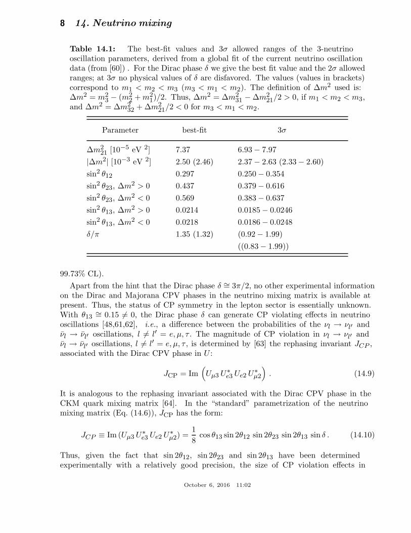
Table 14.1: The best-fit values and 3σ allowed ranges of the 3-neutrinooscillation parameters, derived from a global fit of the current neutrino oscillationdata (from [60]) . For the Dirac phase δ we give the best fit value and the 2σ allowedranges; at 3σ no physical values of δ are disfavored. The values (values in brackets)correspond to m1 < m2 < m3 (m3 < m1 < m2). The definition of ∆m2 used is:∆m2 = m2
3 − (m22 + m2
1)/2. Thus, ∆m2 = ∆m231 − ∆m2
21/2 > 0, if m1 < m2 < m3,and ∆m2 = ∆m2
32 + ∆m221/2 < 0 for m3 < m1 < m2.
Parameter best-fit 3σ
∆m221 [10−5 eV 2] 7.37 6.93 − 7.97
|∆m2| [10−3 eV 2] 2.50 (2.46) 2.37 − 2.63 (2.33 − 2.60)
sin2 θ12 0.297 0.250 − 0.354
sin2 θ23, ∆m2 > 0 0.437 0.379 − 0.616
sin2 θ23, ∆m2 < 0 0.569 0.383 − 0.637
sin2 θ13, ∆m2 > 0 0.0214 0.0185 − 0.0246
sin2 θ13, ∆m2 < 0 0.0218 0.0186 − 0.0248
δ/π 1.35 (1.32) (0.92 − 1.99)
((0.83 − 1.99))
99.73% CL).
Apart from the hint that the Dirac phase δ ∼= 3π/2, no other experimental informationon the Dirac and Majorana CPV phases in the neutrino mixing matrix is available atpresent. Thus, the status of CP symmetry in the lepton sector is essentially unknown.With θ13
∼= 0.15 6= 0, the Dirac phase δ can generate CP violating effects in neutrinooscillations [48,61,62], i.e., a difference between the probabilities of the νl → νl′ andνl → νl′ oscillations, l 6= l′ = e, µ, τ . The magnitude of CP violation in νl → νl′ andνl → νl′ oscillations, l 6= l′ = e, µ, τ , is determined by [63] the rephasing invariant JCP ,associated with the Dirac CPV phase in U :
JCP = Im(
Uµ3 U∗e3 Ue2 U∗
µ2
)
. (14.9)
It is analogous to the rephasing invariant associated with the Dirac CPV phase in theCKM quark mixing matrix [64]. In the “standard” parametrization of the neutrinomixing matrix (Eq. (14.6)), JCP has the form:
JCP ≡ Im (Uµ3 U∗e3 Ue2 U∗
µ2) =1
8cos θ13 sin 2θ12 sin 2θ23 sin 2θ13 sin δ . (14.10)
Thus, given the fact that sin 2θ12, sin 2θ23 and sin 2θ13 have been determinedexperimentally with a relatively good precision, the size of CP violation effects in
October 6, 2016 11:02
14. Neutrino mixing 9
neutrino oscillations depends essentially only on the magnitude of the currently not welldetermined value of the Dirac phase δ. The current data implies JCP . 0.035 sin δ, wherewe have used the 3σ ranges of sin2 θ12, sin2 θ23 and sin2 θ13 given in Table 14.1. For thebest fit values of sin2 θ12, sin2 θ23, sin2 θ13 and δ we find in the case of ∆m2
31(2)> 0
(∆m231(2)
< 0): JCP∼= 0.0327 sin δ ∼= − 0.0291 (JCP
∼= 0.0327 sin δ ∼= − 0.0276). Thus, if
the indication that δ ∼= 3π/2 is confirmed by future more precise data, the CP violationeffects in neutrino oscillations would be relatively large.
If the neutrinos with definite masses νi, i = 1, 2, 3, are Majorana particles, the3-neutrino mixing matrix contains two additional Majorana CPV phases [48]. However,the flavour neutrino oscillation probabilities P (νl → νl′) and P (νl → νl′), l, l′ = e, µ, τ ,do not depend on the Majorana phases [48,65]. The Majorana phases can playimportant role, e.g., in |∆L| = 2 processes like neutrinoless double beta ((ββ)0ν -) decay(A, Z) → (A, Z + 2) + e− + e−, L being the total lepton charge, in which the Majorananature of massive neutrinos νi manifests itself (see, e.g., Refs. [46,66]) . Our interest inthe CPV phases present in the neutrino mixing matrix is stimulated also by the intriguingpossibility that the Dirac phase and/or the Majorana phases in UPMNS can providethe CP violation necessary for the generation of the observed baryon asymmetry of theUniverse [67,68].
As we have indicated, the existing data do not allow one to determine the sign of∆m2
31(2). In the case of 3-neutrino mixing, the two possible signs of ∆m2
31(2)correspond
to two types of neutrino mass spectrum. In the widely used conventions of numbering theneutrinos with definite mass in the two cases, the two spectra read:
– i) spectrum with normal ordering (NO):
m1 < m2 < m3, ∆m231 = ∆m2
A > 0,
∆m221 ≡ ∆m2
⊙ > 0, m2(3) = (m21 + ∆m2
21(31))12 . (14.11)
– ii) spectrum with inverted ordering (IO):
m3 < m1 < m2, ∆m232 = ∆m2
A < 0, ∆m221 ≡ ∆m2
⊙ > 0,
m2 = (m23 + ∆m2
23)12 , m1 = (m2
3 + ∆m223 − ∆m2
21)12 . (14.12)
Depending on the values of the lightest neutrino mass [69], min(mj), the neutrino massspectrum can also be:
– Normal Hierarchical (NH):
m1 ≪ m2 < m3, m2∼= (∆m2
21)12 ∼= 0.0086 eV,
m3∼= |∆m2
31|12 ∼= 0.0504 eV; or (14.13)
– Inverted Hierarchical (IH):
m3 ≪ m1 < m2, m1,2∼= |∆m2
32|12 ∼= 0.0500 eV; or (14.14)
October 6, 2016 11:02
10 14. Neutrino mixing
– Quasi-Degenerate (QD):
m1∼= m2
∼= m3∼= m0, m2
j ≫ |∆m231(32)|, m0 & 0.10 eV. (14.15)
Sometimes the determination of the neutrino mass spectrum is referred to in the literatureon the subject as determination of “neutrino mass hierarchy”. However, as we haveseen, the neutrino mass spectrum might not be hierarchical. Therefore, determinationof “neutrino mass ordering” is a more precise expression and we are going to use thisexpression in the present review article.
Eq. (14.11) and Eq. (14.12) suggest that, for consistency, the data on the largerneutrino mass squared difference, obtained in 3-neutrino oscillation analyses, should bepresented i) either on the value of ∆m2
32 in the case of NO spectrum and on ∆m231 for
IO spectrum, or ii) on the value of ∆m231 for the NO spectrum and on ∆m2
32 for IOspectrum. It would be preferable that all experimental groups which provide data on thelarger neutrino mass squared difference, choose one of the indicated two possibilities topresent their data - this will make straightforward the comparison of the results obtainedin different experiments.
All types of neutrino mass spectrum, discussed above, are compatible with the existingconstraints on the absolute scale of neutrino masses mj . Information about the latter
can be obtained, e.g., by measuring the spectrum of electrons near the end point in 3Hβ-decay experiments [70–74] and from cosmological and astrophysical data. The moststringent upper bounds on the νe mass were obtained in the Troitzk [74,71] experiment:
mνe < 2.05 eV at 95% CL. (14.16)
Similar result was obtained in the Mainz experiment [72]: mνe < 2.3 eV at 95% CL. Wehave mνe
∼= m1,2,3 in the case of QD spectrum. The KATRIN experiment [73] is plannedto reach sensitivity of mνe ∼ 0.20 eV, i.e., it will probe the region of the QD spectrum.
The Cosmic Microwave Background (CMB) data of the WMAP experiment, combinedwith supernovae data and data on galaxy clustering can be used to obtain an upper limiton the sum of neutrinos masses (see review on Cosmological Parameters [75] and, e.g.,Ref. 76). Depending on the model complexity and the input data used one obtains [76]:∑
j mj . (0.3 − 1.3) eV, 95% CL.
In March of 2013 the Planck Collaboration published their first constraints on∑
j mj [77]. These constraints were updated in 2015 in [78]. Assuming the existence of
three light massive neutrinos and the validity of the Λ CDM (Cold Dark Matter) model,and using their data on the CMB temperature power spectrum anisotropies, polarization,on gravitational lensing effects and the low l CMB polarization spectrum data (the“low P” data), the Planck Collaboration reported the following updated upper limit onthe sum of the neutrino masses [78]:
∑
j mj < 0.57 eV, 95% CL. Adding supernovae
(light-curve) data and data on the Baryon Acoustic Oscillations (BAO) lowers the limitto [78]:
∑
j
mj < 0.23 eV, 95% CL.
October 6, 2016 11:02
14. Neutrino mixing 11
It follows from these data that neutrino masses are much smaller than the masses ofcharged leptons and quarks. If we take as an indicative upper limit mj . 0.5 eV, we have
mj/ml,q . 10−6, l = e, µ, τ , q = d, s, b, u, c, t. It is natural to suppose that the remarkablesmallness of neutrino masses is related to the existence of a new fundamental mass scalein particle physics, and thus to new physics beyond that predicted by the StandardModel.
14.3. Future progress
After the spectacular experimental progress made in the studies of neutrino oscillations,further understanding of the pattern of neutrino masses and neutrino mixing, of theirorigins and of the status of CP symmetry in the lepton sector requires an extensive andchallenging program of research. The main goals of such a research program include:
• Determining the nature - Dirac or Majorana, of massive neutrinos νj . This is offundamental importance for making progress in our understanding of the origin ofneutrino masses and mixing and of the symmetries governing the lepton sector ofparticle interactions.
• Determination of the sign of ∆m231 (or ∆m2
32), i.e., the “neutrino mass ordering”, orof the type of spectrum neutrino masses obey.
• Determining, or obtaining significant constraints on, the absolute scale of neutrinomasses. This, in particular, would help obtain information about the detailedstructure (hierarchical, quasidegenerate, etc.) of the neutrino mass spectrum.
• Determining the status of CP symmetry in the lepton sector.
• High precision measurement of θ13, ∆m221, θ12, |∆m2
31| and θ23.
• Understanding at a fundamental level the mechanism giving rise to neutrino massesand mixing and to Ll−non-conservation. This includes understanding the origin ofthe patterns of ν-mixing and ν-masses suggested by the data. Are the observedpatterns of ν-mixing and of ∆m2
21,31 related to the existence of a new fundamentalsymmetry of particle interactions? Is there any relation between quark mixing andneutrino mixing, e.g., does the relation θ12 + θc=π/4, where θc is the Cabibbo angle,hold? What is the physical origin of CP violation phases in the neutrino mixingmatrix U? Is there any relation (correlation) between the (values of) CP violationphases and mixing angles in U? Progress in the theory of neutrino mixing might alsolead to a better understanding of the mechanism of generation of baryon asymmetryof the Universe.
The high precision measurement of the value of sin2 2θ13 from the Daya Bay experimentand the subsequent results on θ13 obtained by the RENO, Double Chooz and T2Kcollaborations (see Section 1.11), have far reaching implications. The measured relativelylarge value of θ13 opened up the possibilities, in particular,
i) for searching for CP violation effects in neutrino oscillation experiments with highintensity accelerator neutrino beams, like T2K, NOνA, etc. The sensitivities of T2K andNOνA on CP violation in neutrino oscillations are discussed in, e.g., Refs. [79,80]. ii) fordetermining the sign of ∆m2
32, and thus the type of neutrino mass spectrum (“neutrino
October 6, 2016 11:02
12 14. Neutrino mixing
mass ordering”) in the long baseline neutrino oscillation experiments at accelerators(NOνA, etc.), in the experiments studying the oscillations of atmospheric neutrinos(PINGU, ORCA), as well as in experiments with reactor antineutrinos [81] (for a reviewsee, e.g., Ref. 82).
There are also long term plans extending beyond 2025 for searches for CP violationand neutrino mass spectrum (ordering) determination in long baseline neutrino oscillationexperiments with accelerator neutrino beams (see, e.g., Refs. [80,83,84,85]) . Thesuccessful realization of this research program would be a formidable task and wouldrequire many years of extraordinary experimental efforts aided by intensive theoreticalinvestigations and remarkable investments.
Before reviewing in detail i) the different neutrino sources and the specific characteristicsof the corresponding neutrino fluxes, which have been and are being used in neutrinooscillation experiments (Section 14.6), ii) the theory and phenomenology of neutrinooscillations (Sections 14.7 and 14.8), and iii) the compelling experimental evidences ofneutrino oscillations and, more generally, the results obtained in the neutrino oscillationexperiments (Sections 14.9 and 14.13), we would like to discuss briefly the problem ofdetermination of the nature - Dirac or Majorana - of massive neutrinos as well as the(type I) seesaw mechanism of neutrino mass generation.
14.4. The nature of massive neutrinos
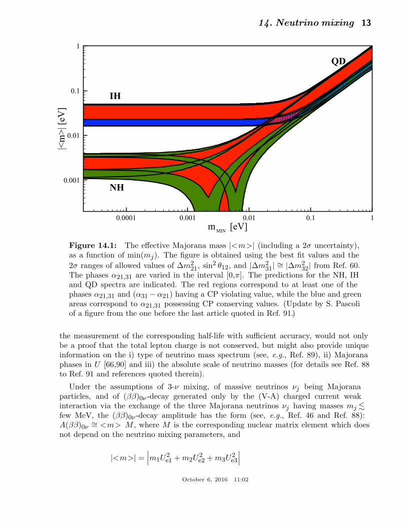
The experiments studying flavour neutrino oscillations cannot provide information onthe nature - Dirac or Majorana, of massive neutrinos [48,65]. Establishing whether theneutrinos with definite mass νj are Dirac fermions possessing distinct antiparticles, orMajorana fermions, i.e., spin 1/2 particles that are identical with their antiparticles, isof fundamental importance for understanding the origin of ν-masses and mixing andthe underlying symmetries of particle interactions (see, e.g., Ref. 86). The neutrinoswith definite mass νj will be Dirac fermions if the particle interactions conserve someadditive lepton number, e.g., the total lepton charge L = Le + Lµ + Lτ . If no leptoncharge is conserved, νj will be Majorana fermions (see, e.g., Ref. 46). The massiveneutrinos are predicted to be of Majorana nature by the see-saw mechanism of neutrinomass generation [3]. The observed patterns of neutrino mixing and of neutrino masssquared differences can be related to Majorana massive neutrinos and the existence of anapproximate flavour symmetry in the lepton sector (see, e.g., Ref. 87). Determining thenature of massive neutrinos νj is one of the fundamental and most challenging problemsin the future studies of neutrino mixing.
The Majorana nature of massive neutrinos νj manifests itself in the existence ofprocesses in which the total lepton charge L changes by two units: K+ → π− + µ+ + µ+,µ− + (A, Z) → µ+ + (A, Z − 2), etc. Extensive studies have shown that the onlyfeasible experiments having the potential of establishing that the massive neutrinosare Majorana particles are at present the experiments searching for (ββ)0ν -decay:(A, Z) → (A, Z + 2) + e− + e− (see, e.g., Ref. 88). The observation of (ββ)0ν -decay and
October 6, 2016 11:02
14. Neutrino mixing 13
!"!!!# !"!!# !"!# !"# #
$%%%%%%&'()
!"!!#
!"!#
!"#
#
*+$,*%&'()
!"
#"
$%
-./!
Figure 14.1: The effective Majorana mass |<m>| (including a 2σ uncertainty),as a function of min(mj). The figure is obtained using the best fit values and the
2σ ranges of allowed values of ∆m221, sin2 θ12, and |∆m2
31| ∼= |∆m232| from Ref. 60.
The phases α21,31 are varied in the interval [0,π]. The predictions for the NH, IHand QD spectra are indicated. The red regions correspond to at least one of thephases α21,31 and (α31 −α21) having a CP violating value, while the blue and greenareas correspond to α21,31 possessing CP conserving values. (Update by S. Pascoliof a figure from the one before the last article quoted in Ref. 91.)
the measurement of the corresponding half-life with sufficient accuracy, would not onlybe a proof that the total lepton charge is not conserved, but might also provide uniqueinformation on the i) type of neutrino mass spectrum (see, e.g., Ref. 89), ii) Majoranaphases in U [66,90] and iii) the absolute scale of neutrino masses (for details see Ref. 88to Ref. 91 and references quoted therein).
Under the assumptions of 3-ν mixing, of massive neutrinos νj being Majoranaparticles, and of (ββ)0ν -decay generated only by the (V-A) charged current weakinteraction via the exchange of the three Majorana neutrinos νj having masses mj .
few MeV, the (ββ)0ν -decay amplitude has the form (see, e.g., Ref. 46 and Ref. 88):A(ββ)0ν
∼= <m> M , where M is the corresponding nuclear matrix element which doesnot depend on the neutrino mixing parameters, and
|<m>| =∣
∣
∣m1U
2e1 + m2U
2e2 + m3U
2e3
∣
∣
∣
October 6, 2016 11:02
14 14. Neutrino mixing
=∣
∣
∣
(
m1c212 + m2s
212e
iα21)
c213 + m3s213e
i(α31−2δ)∣
∣
∣, (14.17)
is the effective Majorana mass in (ββ)0ν -decay. In the case of CP-invariance one has [50],η21 ≡ eiα21=±1, η31 ≡ eiα31=±1, e−i2δ=1. The three neutrino masses m1,2,3 can be
expressed in terms of the two measured ∆m2jk and, e.g., min(mj). Thus, given the
neutrino oscillation parameters ∆m221, sin2 θ12, ∆m2
31 and sin2 θ13, |<m>| is a functionof the lightest neutrino mass min(mj), the Majorana (and Dirac) CP violation phases inU and of the type of neutrino mass spectrum. In the case of NH, IH and QD spectrumwe have (see, e.g., Ref. 66 and Ref. 91):
|<m>| ∼=∣
∣
∣
∣
√
∆m221s
212c
213 +
√
∆m231s
213e
i(α31−α21−2δ)
∣
∣
∣
∣
, NH , (14.18)
|<m>| ∼= m(
1 − sin2 2θ12 sin2 α21
2
)12
, IH (IO) and QD , (14.19)
where m ≡√
∆m223 + m2
3 and m ≡ m0 for IH (IO) and QD spectrum, respectively.
In Eq. (14.19) we have exploited the fact that sin2 θ13 ≪ cos 2θ12. The CP con-serving values of the Majorana phase α21 and the Majorana-Dirac phase difference(α31 − α21 − 2δ) determine the intervals of possible values of |<m>|, correspond-ing to the different types of neutrino mass spectrum. Using the 3σ ranges of theallowed values of the neutrino oscillation parameters from Table 14.1 one findsthat: i) 0.81 × 10⁻³ eV . |<m>|. 4.43 × 10⁻³ eV in the case of NH spectrum; ii)√
∆m223 cos 2θ12 c213 . |<m>|.
√
∆m223 c213, or 1.3 × 10⁻² eV . |<m>|. 5.0 × 10⁻² eV
in the case of IH spectrum; 1.3 × 10⁻² eV . |<m>|. 5.0 × 10⁻² eV in the case of IHspectrum; iii) m0 cos 2θ12 . |<m>|.m0, or 2.9× 10⁻² eV . |<m>|.m0 eV, m0 & 0.10eV, in the case of QD spectrum. The difference in the ranges of |<m>| in the casesof NH, IH and QD spectrum opens up the possibility to get information about thetype of neutrino mass spectrum from a measurement of |<m>| [89]. The predicted(ββ)0ν -decay effective Majorana mass |<m>| as a function of the lightest neutrino massmin(mj) is shown in Fig. 14.1.
The (ββ)0ν -decay can be generated, in principle, by a ∆L = 2 mechanism otherthan the light Majorana neutrino exchange considered here, or by a combination ofmechanisms one of which is the light Majorana neutrino exchange (for a discussion ofdifferent mechanisms which can trigger (ββ)0ν -decay, see, e.g., Refs. [92,93] and thearticles quoted therein). If the (ββ)0ν -decay will be observed, it will be of fundamentalimportance to determine which mechanism (or mechanisms) is (are) inducing the decay.The discussion of the problem of determining the mechanisms which possibly are operativein (ββ)0ν -decay, including the case when more than one mechanism is involved, is outof the scope of the present article. This problem has been investigated in detail in, e.g.,Refs. [93,94] and we refer the reader to these articles and the articles quoted therein.
October 6, 2016 11:02
14. Neutrino mixing 15
14.5. The see-saw mechanism and the baryon asymmetry of the
Universe
A natural explanation of the smallness of neutrino masses is provided by the (typeI) see-saw mechanism of neutrino mass generation [3]. An integral part of this rathersimple mechanism [95] are the RH neutrinos νlR (RH neutrino fields νlR(x)). The latterare assumed to possess a Majorana mass term as well as Yukawa type coupling LY(x)with the Standard Model lepton and Higgs doublets, ψlL(x) and Φ(x), respectively,
(ψlL(x))T = (νTlL(x) lTL(x)), l = e, µ, τ , (Φ(x))T = (Φ(0)(x) Φ(−)(x)). In the basis in
which the Majorana mass matrix of RH neutrinos is diagonal, we have:
LY,M(x) =(
λil NiR(x) Φ†(x) ψlL(x) + h.c.)
− 1
2Mi Ni(x) Ni(x) , (14.20)
where λil is the matrix of neutrino Yukawa couplings and Ni (Ni(x)) is the heavy RHMajorana neutrino (field) possessing a mass Mi > 0. When the electroweak symmetryis broken spontaneously, the neutrino Yukawa coupling generates a Dirac mass term:mD
il NiR(x) νlL(x) + h.c., with mD = vλ, v = 174 GeV being the Higgs doublet v.e.v. In
the case when the elements of mD are much smaller than Mk, |mDil | ≪ Mk, i, k = 1, 2, 3,
l = e, µ, τ , the interplay between the Dirac mass term and the mass term of the heavy(RH) Majorana neutrinos Ni generates an effective Majorana mass (term) for the LHflavour neutrinos [3]:
mLLl′l
∼= −(mD)Tl′jM−1j mD
jl = −v2(λ)Tl′jM−1j λjl . (14.21)
In grand unified theories, mD is typically of the order of the charged fermion masses.In SO(10) theories, for instance, mD coincides with the up-quark mass matrix. Takingindicatively mLL ∼ 0.1 eV, mD ∼ 100 GeV, one finds M ∼ 1014 GeV, which is close tothe scale of unification of the electroweak and strong interactions, MGUT
∼= 2× 10¹⁶ GeV.In GUT theories with RH neutrinos one finds that indeed the heavy Majorana neutrinosNj naturally obtain masses which are by few to several orders of magnitude smaller thanMGUT . Thus, the enormous disparity between the neutrino and charged fermion massesis explained in this approach by the huge difference between effectively the electroweaksymmetry breaking scale and MGUT .
An additional attractive feature of the see-saw scenario is that the generation andsmallness of neutrino masses is related via the leptogenesis mechanism [2] to thegeneration of the baryon asymmetry of the Universe. The Yukawa coupling in Eq. (14.20),in general, is not CP conserving. Due to this CP-nonconserving coupling the heavyMajorana neutrinos undergo, e.g., the decays Nj → l+ + Φ(−), Nj → l− + Φ(+), which
have different rates: Γ(Nj → l+ + Φ(−)) 6= Γ(Nj → l− + Φ(+)). When these decays occurin the Early Universe at temperatures somewhat below the mass of, say, N1, so that thelatter are out of equilibrium with the rest of the particles present at that epoch, CPviolating asymmetries in the individual lepton charges Ll, and in the total lepton chargeL, of the Universe are generated. These lepton asymmetries are converted into a baryon
October 6, 2016 11:02
16 14. Neutrino mixing
asymmetry by (B−L) conserving, but (B +L) violating, sphaleron processes, which existin the Standard Model and are effective at temperatures T ∼ (100 − 1012) GeV. If theheavy neutrinos Nj have hierarchical spectrum, M1 ≪ M2 ≪ M3, the observed baryon
asymmetry can be reproduced provided the mass of the lightest one satisfies M1 & 109
GeV [96]. Thus, in this scenario, the neutrino masses and mixing and the baryonasymmetry have the same origin - the neutrino Yukawa couplings and the existence of(at least two) heavy Majorana neutrinos. Moreover, quantitative studies [67] based onadvances in leptogenesis theory [97] have shown that the CP violation, necessary inleptogenesis for the generation of the observed baryon asymmetry of the Universe, canbe provided exclusively by the Dirac and/or Majorana phases in the neutrino mixingmatrix U . This implies, in particular, that if the CP symmetry is established not to holdin the lepton sector due to U , at least some fraction (if not all) of the observed baryonasymmetry might be due to the Dirac and/or Majorana CP violation present in theneutrino mixing. More specifically, the necessary condition that the requisite CP violationfor a successful leptogenesis with heirarchical in mass heavy Majorana neutrinos is dueentirely to the Dirac CPV phase in U reads [68]: | sin θ13 sin δ|& 0.09. This conditionis comfortably compatible with the measured value of sin θ13
∼= 0.15 and the hint thatδ ∼= 3π/2, found in the global analyses of the neutrino oscillation data.
14.6. Neutrino sources
In the experimental part of this review (Sections 14.9 - 14.13), we mainly discussneutrino oscillation experiments using neutrinos or antineutrinos produced by the Sun,cosmic-ray interactions in the air, proton accelerators, and nuclear reactors. We callneutrinos from these sources as solar neutrinos, atmospheric neutrinos, acceleratorneutrinos, and reactor (anti)neutrinos. Neutrinos (and/or antineutrinos) from each ofthese sources have very different properties, e.g., energy spectra, flavour components, anddirectional distributions, at production. In the literature, neutrino flavour conversion ofneutrinos from gravitationally collapsed supernova explosions (supernova neutrinos) isalso discussed, but this topic is out of the scope of the present review.
Solar neutrinos and atmospheric neutrinos are naturally produced neutrinos; theirfluxes as well as the distance between the (point or distributed) neutrino source and thedetector cannot be controlled artificially. While the atmospheric neutrino flux involves νµ,νµ, νe, and νe components at production, solar neutrinos are produced as pure electronneutrinos due to thermo-nuclear fusion reactions of four protons, producing a heliumnucleus. For atmospheric neutrinos with energy & 1 GeV, which undergo charged-currentinteractions in the detector, directional correlation of the charged lepton with the parentneutrino gives the way to know, within the resolution, the distance traveled by theneutrino between the production and detection.
Accelerator neutrinos and reactor (anti)neutrinos are man-made neutrinos. Inprinciple, it is possible to choose the distance between the neutrino source and thedetector arbitrarily. Accelerator neutrinos used for neutrino oscillation experiments so farhave been produced by the decay of secondary mesons (pions and kaons) produced by thecollision of a primary proton beam with a nuclear target. A dominant component of the
October 6, 2016 11:02
14. Neutrino mixing 17
accelerator neutrino flux is νµ or νµ, depending on the secondary meson’s sign selection,but a wrong-sign muon neutrino component as well as νe and νe components are alsopresent. The fluxes of the accelerator neutrinos depend on a number of factors, e.g.,energy and intensity of the primary proton beam, material and geometry of the target,selection of the momentum and charge of the secondary mesons that are focused, andproduction angle of the secondary mesons with respect to the primary beam. In otherwords, it is possible to control the peak energy, energy spread, and dominant neutrinoflavour, of the neutrino beam.
From the nuclear reactor, almost pure electron antineutrinos are produced by β-decaysof fission products of the nuclear fuel. However, experimental groups cannot control thenormalization and spectrum of the νe flux from commercial nuclear reactors. They aredependent on the initial fuel composition and history of the nuclear fuel burnup. Thesedata are provided by the power plant companies.
For neutrino oscillation experiments, knowledge of the flux of each neutrino andantineutrino flavour at production is needed for planning and designing the experiment,analyzing the data, and estimating systematic errors. Basically, for all neutrino sources,flux models are constructed and validation is made by comparing various experimentallyobserved quantities with the model predictions. Many of the modern accelerator longbaseline and reactor neutrino oscillation experiments employ a two- or multi-detectorconfiguration. In the accelerator long baseline experiment, a “near” detector measuresnon-oscillated neutrino flux. In the two- or multi-baseline reactor experiments, even anear detector measures the neutrino flux with oscillations developed to some extent.However, comparing the quantities measured with different baselines, it is possible tovalidate the reactor flux model and measure the oscillation parameters at the same time,or to make an analysis with minimal dependence on flux models.
14.6.1. Standard solar model predictions of the solar neutrino fluxes :
Observation of solar neutrinos directly addresses the theory of stellar structureand evolution, which is the basis of the standard solar model (SSM). The Sun, as awell-defined neutrino source, also provides an important opportunities to investigateneutrino oscillations including matter effects, because of the wide range of matter densityand the great distance from the Sun to the Earth.
The solar neutrinos are produced by some of the fusion reactions in the pp chain orCNO cycle. The combined effect of these reactions is written as
4p → 4He + 2e+ + 2νe. (14.22)
Positrons annihilate with electrons. Therefore, when considering the solar thermal energygeneration, a relevant expression is
4p + 2e− → 4He + 2νe + 26.73 MeV − Eν , (14.23)
where Eν represents the energy taken away by neutrinos, the average value being〈Eν〉 ∼ 0.6 MeV. There have been efforts to calculate solar neutrino fluxes from these
October 6, 2016 11:02
18 14. Neutrino mixing
Table 14.2: Neutrino-producing reactions in the Sun (first column) and theirabbreviations (second column). The neutrino fluxes predicted by the BPS08(GS)model [100] are listed in the third column.
Reaction Abbr. Flux (cm−2 s−1)
pp → d e+ ν pp 5.97(1± 0.006) × 1010
pe−p → d ν pep 1.41(1± 0.011) × 108
3He p → 4He e+ν hep 7.90(1± 0.15) × 103
7Be e− → 7Li ν + (γ) 7Be 5.07(1± 0.06) × 109
8B → 8Be∗ e+ν 8B 5.94(1± 0.11) × 106
13N → 13C e+ν 13N 2.88(1± 0.15) × 108
15O → 15N e+ν 15O 2.15(1+0.17−0.16) × 108
17F → 17O e+ν 17F 5.82(1+0.19−0.17) × 106
Figure 14.2: The solar neutrino spectrum predicted by the BPS08(GS) standardsolar model [100]. The neutrino fluxes are given in units of cm−2s−1MeV−1 forcontinuous spectra and cm−2s−1 for line spectra. The numbers associated with theneutrino sources show theoretical errors of the fluxes. This figure is taken from AldoSerenelli’s web site, http://www.mpa-garching.mpg.de/~aldos/.
October 6, 2016 11:02
14. Neutrino mixing 19
reactions on the basis of SSM. A variety of input information is needed in the evolutionarycalculations. The most elaborate SSM calculations have been developed by Bahcalland his collaborators, who define their SSM as the solar model which is constructedwith the best available physics and input data. Therefore, their SSM calculations havebeen rather frequently updated. SSM’s labelled as BS05(OP) [98], BSB06(GS) andBSB06(AGS) [99], and BPS08(GS) and BPS08(AGS) [100] represent some of therelatively recent model calculations. Here, “OP” means that newly calculated radiativeopacities from the “Opacity Project” are used. The later models are also calculated withOP opacities. “GS” and “AGS” refer to old and new determinations of solar abundancesof heavy elements. There are significant differences between the old, higher heavy elementabundances (GS) and the new, lower heavy element abundances (AGS). The models withGS are consistent with helioseismological data, but the models with AGS are not.
The prediction of the BPS08(GS) model for the fluxes from neutrino-producingreactions is given in Table 14.2. Fig. 14.2 shows the solar-neutrino spectra calculatedwith the BPS08(GS) model. Here we note that in Ref. 101 the authors point out thatelectron capture on 13N, 15O, and 17F produces line spectra of neutrinos, which have notbeen considered in the SSM calculations quoted above.
In 2011, a new SSM calculations [102] have been presented by A.M. Serenelli, W.C.Haxton, and C. Pena-Garay, by adopting the newly analyzed nuclear fusion cross sections.Their high metalicity SSM is labelled as SHP11(GS). For the same solar abundances asused in Ref. 98 and Ref. 99, the most significant change is a decrease of 8B flux by ∼ 5%.
14.6.2. Atmospheric neutrino fluxes :
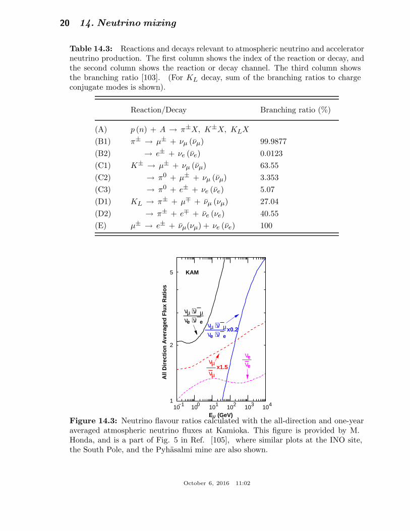
Atmospheric neutrinos are produced by the decay of π and K mesons produced in thenuclear interactions of the primary component of cosmic rays in the atmosphere ((A)in Table 14.3). The primary cosmic ray components above 2 GeV/nucleon are protons(∼ 95%), helium nuclei (∼ 4.5%), and heavier nuclei. For neutrino producing hadronicinteractions, a nucleus can be simply regarded as a sum of individual nucleons at highenergies. Pions are dominantly produced in these interactions, and they predominantlydecay according to (B1) in Table 14.3, followed by muon decay (E) in Table 14.3. Theinteractions in massive underground detectors of atmospheric neutrinos provide a meansof studying neutrino oscillations because of the large range of distances traveled bythese neutrinos (∼10 to 1.27 × 10⁴ km) to reach a detector on Earth and relativelywell-understood atmospheric neutrino fluxes.
Calculation of the atmospheric neutrino fluxes requires knowledge of the primarycosmic-ray fluxes and composition, and the hadronic interactions. Atmospheric neutrinoswith energy of ∼a few GeV are mostly produced by primary cosmic rays with energyof ∼100 GeV. For primary cosmic-rays in this energy range, a flux modulation due tothe solar activity and the effects of Earth’s geomagnetic fields should be taken intoaccount. In particular, the atmospheric neutrino fluxes in the low-energy region dependon the location on the Earth. Detailed calculations of the atmospheric neutrino fluxes areperformed by Honda et al. [104,105], Barr et al. [106], and Battistoni et al. [107], witha typical uncertainty of 10 ∼ 20%.
October 6, 2016 11:02
20 14. Neutrino mixing
Table 14.3: Reactions and decays relevant to atmospheric neutrino and acceleratorneutrino production. The first column shows the index of the reaction or decay, andthe second column shows the reaction or decay channel. The third column showsthe branching ratio [103]. (For KL decay, sum of the branching ratios to chargeconjugate modes is shown).
Reaction/Decay Branching ratio (%)
(A) p (n) + A → π±X, K±X, KLX
(B1) π± → µ± + νµ (νµ) 99.9877
(B2) → e± + νe (νe) 0.0123
(C1) K± → µ± + νµ (νµ) 63.55
(C2) → π0 + µ± + νµ (νµ) 3.353
(C3) → π0 + e± + νe (νe) 5.07
(D1) KL → π± + µ∓ + νµ (νµ) 27.04
(D2) → π± + e∓ + νe (νe) 40.55
(E) µ± → e± + νµ(νµ) + νe (νe) 100
E (GeV)ν
eν + νµν + ν
x0.2e
µ
µν
µν
eν + νµ
eνeν
µe
ν + ν
x1.5
All
Dire
ctio
n A
vera
ged
Flu
x R
atio
s
KAM
10 −1 100 10 1 10 2 10 3 10 41
2
5
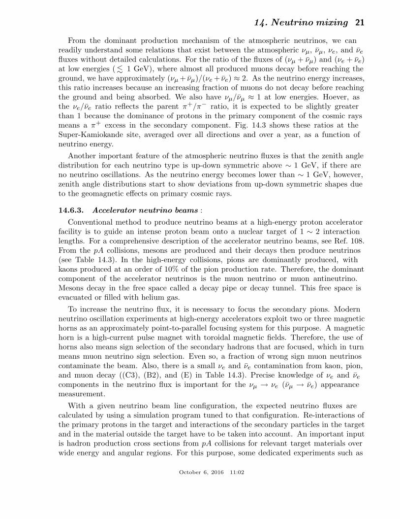
Figure 14.3: Neutrino flavour ratios calculated with the all-direction and one-yearaveraged atmospheric neutrino fluxes at Kamioka. This figure is provided by M.Honda, and is a part of Fig. 5 in Ref. [105], where similar plots at the INO site,the South Pole, and the Pyhasalmi mine are also shown.
October 6, 2016 11:02
14. Neutrino mixing 21
From the dominant production mechanism of the atmospheric neutrinos, we canreadily understand some relations that exist between the atmospheric νµ, νµ, νe, and νe
fluxes without detailed calculations. For the ratio of the fluxes of (νµ + νµ) and (νe + νe)at low energies ( . 1 GeV), where almost all produced muons decay before reaching theground, we have approximately (νµ + νµ)/(νe + νe) ≈ 2. As the neutrino energy increases,this ratio increases because an increasing fraction of muons do not decay before reachingthe ground and being absorbed. We also have νµ/νµ ≈ 1 at low energies. Hoever, asthe νe/νe ratio reflects the parent π+/π− ratio, it is expected to be slightly greaterthan 1 because the dominance of protons in the primary component of the cosmic raysmeans a π+ excess in the secondary component. Fig. 14.3 shows these ratios at theSuper-Kamiokande site, averaged over all directions and over a year, as a function ofneutrino energy.
Another important feature of the atmospheric neutrino fluxes is that the zenith angledistribution for each neutrino type is up-down symmetric above ∼ 1 GeV, if there areno neutrino oscillations. As the neutrino energy becomes lower than ∼ 1 GeV, however,zenith angle distributions start to show deviations from up-down symmetric shapes dueto the geomagnetic effects on primary cosmic rays.
14.6.3. Accelerator neutrino beams :
Conventional method to produce neutrino beams at a high-energy proton acceleratorfacility is to guide an intense proton beam onto a nuclear target of 1 ∼ 2 interactionlengths. For a comprehensive description of the accelerator neutrino beams, see Ref. 108.From the pA collisions, mesons are produced and their decays then produce neutrinos(see Table 14.3). In the high-energy collisions, pions are dominantly produced, withkaons produced at an order of 10% of the pion production rate. Therefore, the dominantcomponent of the accelerator neutrinos is the muon neutrino or muon antineutrino.Mesons decay in the free space called a decay pipe or decay tunnel. This free space isevacuated or filled with helium gas.
To increase the neutrino flux, it is necessary to focus the secondary pions. Modernneutrino oscillation experiments at high-energy accelerators exploit two or three magnetichorns as an approximately point-to-parallel focusing system for this purpose. A magnetichorn is a high-current pulse magnet with toroidal magnetic fields. Therefore, the use ofhorns also means sign selection of the secondary hadrons that are focused, which in turnmeans muon neutrino sign selection. Even so, a fraction of wrong sign muon neutrinoscontaminate the beam. Also, there is a small νe and νe contamination from kaon, pion,and muon decay ((C3), (B2), and (E) in Table 14.3). Precise knowledge of νe and νe
components in the neutrino flux is important for the νµ → νe (νµ → νe) appearancemeasurement.
With a given neutrino beam line configuration, the expected neutrino fluxes arecalculated by using a simulation program tuned to that configuration. Re-interactions ofthe primary protons in the target and interactions of the secondary particles in the targetand in the material outside the target have to be taken into account. An important inputis hadron production cross sections from pA collisions for relevant target materials overwide energy and angular regions. For this purpose, some dedicated experiments such as
October 6, 2016 11:02
22 14. Neutrino mixing
SPY [109], HARP [110], MIPP [111], and NA61/SHINE [112] have been conducted.The data are fit to specific hadron production models to determine the model parameters.
The predicted neutrino fluxes have to be validated in some way. Modern long baselineneutrino oscillation experiments often have a two-detector configuration, with a neardetector to measure an unoscillated neutrino flux immediately after the production. Inthe single detector experiment, the muon-neutrino flux model is calibrated by using amuon monitor which is located behind the beam dump. Since low-energy muons areabsorbed in the beam dump, it is not possible to calibrate the low-energy part of theneutrino spectrum. Even in the two-detector experiments, it should be noted that thenear detector does not see the same neutrino flux as the far detector sees, because theneutrino source looks like a line source for the near detector, while it looks as a pointsource for the far detector.
The energy Eν of the neutrino emitted at an angle θ with respect to the parent piondirection is given by
Eν =m2
π − m2µ
2(Eπ − pπcosθ), (14.24)
where Eπ and pπ are the energy and momentum of the parent pion, mπ is the chargedpion mass, mµ is the muon mass. Suppose an ideal case that the pions are completelyfocused in parallel. Then, for θ = 0, it can be seen from the above equation that Eν isproportional to Eπ for Eπ ≫ mπ . As the secondary pions have a wide energy spectrum,a 0 degree neutrino beam also has a wide spectrum and is called a “wide-band beam”.
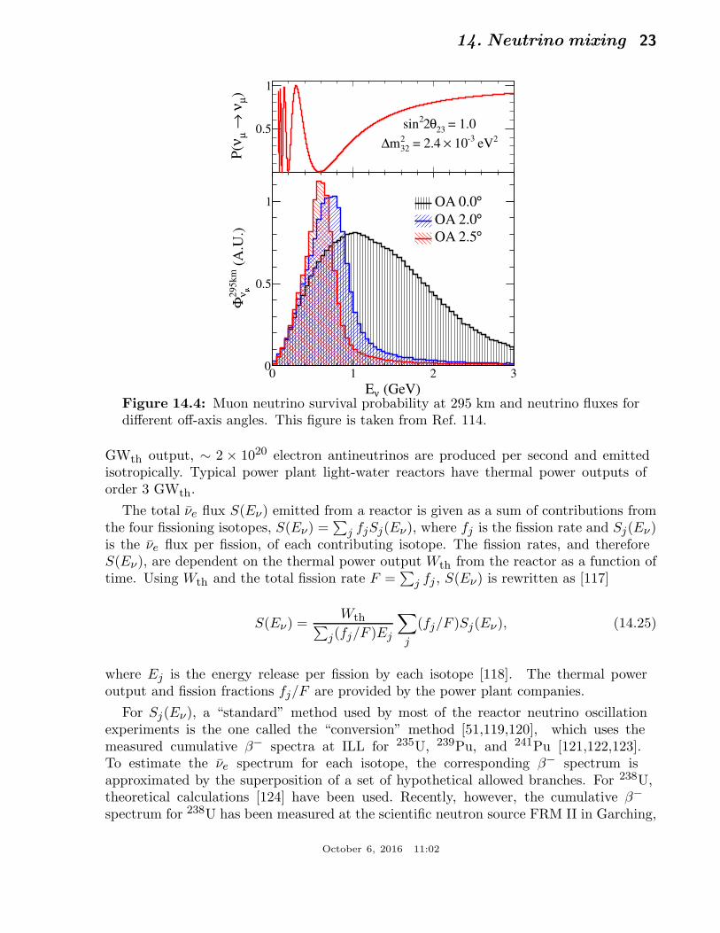
For a given angle θ, differentiating the above expression with respect to Eπ, it can beshown that Eν takes a maximum value Emax
ν = (m2π −m2
µ)/(2E◦πsin2θ) at E◦
π = mπ/sinθ.Numerical calculations show that a wide range of Eπ, in particular that of Eπ ≥ E◦
π,contributes to a narrow range of Eν ≤ Emax
ν [113]. It is expected, therefore, that anarrow neutrino spectrum peaked at around Emax
ν can be obtained by the off-axis beam.Fig. 14.4 shows an example of the simulated muon neutrino fluxes at θ = 0 degree and2.0◦ and 2.5◦ off-axis configurations corresponding to the T2K experiment [114]. Asexpected, an off-axis beam has a narrower spectrum than the 0 degree wide-band beam.Therefore, an off-axis beam is called a “narrow-band beam”. This idea of an off-axisbeam was proposed for BNL E889 experiment [113]. It has been employed for the T2Kexperiment for the first time. Currently, it is also used in the NOνA experiment [115].For the off-axis beam, obviously the effect of a line neutrino source, namely the differencebetween the neutrino fluxes measured at the near and far detectors, is enhanced, and ithas to be properly taken into account.
14.6.4. Reactor neutrino fluxes :
In nuclear reactors, power is generated mainly by nuclear fission of four heavy isotopes,235U, 238U, 239Pu, and 241Pu. These isotopes account for more than 99% of fissionsin the reactor core. β-decays of fission products produce almost pure νe flux. The rateof νe production is less than 10−5 of the rate of νe production [116]. The thermalpower outputs of nuclear power reactors are usually quoted in thermal GW, GWth. Onthe average, ∼ 200 MeV and 6 electron antineutrinos are emitted per fission. With 1
October 6, 2016 11:02
14. Neutrino mixing 23
Figure 14.4: Muon neutrino survival probability at 295 km and neutrino fluxes fordifferent off-axis angles. This figure is taken from Ref. 114.
GWth output, ∼ 2 × 10²⁰ electron antineutrinos are produced per second and emittedisotropically. Typical power plant light-water reactors have thermal power outputs oforder 3 GWth.
The total νe flux S(Eν) emitted from a reactor is given as a sum of contributions fromthe four fissioning isotopes, S(Eν) =
∑
j fjSj(Eν), where fj is the fission rate and Sj(Eν)is the νe flux per fission, of each contributing isotope. The fission rates, and thereforeS(Eν), are dependent on the thermal power output Wth from the reactor as a function oftime. Using Wth and the total fission rate F =
∑
j fj , S(Eν) is rewritten as [117]
S(Eν) =Wth
∑
j(fj/F )Ej
∑
j
(fj/F )Sj(Eν), (14.25)
where Ej is the energy release per fission by each isotope [118]. The thermal poweroutput and fission fractions fj/F are provided by the power plant companies.
For Sj(Eν), a “standard” method used by most of the reactor neutrino oscillationexperiments is the one called the “conversion” method [51,119,120], which uses themeasured cumulative β− spectra at ILL for 235U, 239Pu, and 241Pu [121,122,123].To estimate the νe spectrum for each isotope, the corresponding β− spectrum isapproximated by the superposition of a set of hypothetical allowed branches. For 238U,theoretical calculations [124] have been used. Recently, however, the cumulative β−
spectrum for 238U has been measured at the scientific neutron source FRM II in Garching,
October 6, 2016 11:02
24 14. Neutrino mixing
Eν (MeV)
(see
ann
otat
ions
)
(a)
(b)
(c)
a) ν_
e interactions in detector [1/(day MeV)]
b) ν_
e flux at detector [108/(s MeV cm2)]
c) σ(Eν) [10-43 cm2]
0
10
20
30
40
50
60
70
80
90
100
2 3 4 5 6 7 8 9 10
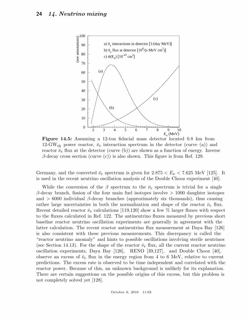
Figure 14.5: Assuming a 12-ton fiducial mass detector located 0.8 km from12-GWth power reactor, νe interaction spectrum in the detector (curve (a)) andreactor νe flux at the detector (curve (b)) are shown as a function of energy. Inverseβ-decay cross section (curve (c)) is also shown. This figure is from Ref. 129.
Germany, and the converted νe spectrum is given for 2.875 < Eν < 7.625 MeV [125]. Itis used in the recent neutrino oscillation analysis of the Double Chooz experiment [40].
While the conversion of the β spectrum to the νe spectrum is trivial for a singleβ-decay branch, fission of the four main fuel isotopes involve > 1000 daughter isotopesand > 6000 individual β-decay branches (approximately six thousands), thus causingrather large uncertainties in both the normalization and shape of the reactor νe flux.Recent detailed reactor νe calculations [119,120] show a few % larger fluxes with respectto the fluxes calculated in Ref. 122. The antineutrino fluxes measured by previous shortbaseline reactor neutrino oscillation experiments are generally in agreement with thelatter calculation. The recent reactor antineutrino flux measurement at Daya Bay [126]is also consistent with these previous measurements. This discrepancy is called the“reactor neutrino anomaly” and hints to possible oscillations involving sterile neutrinos(see Section 14.13). For the shape of the reactor νe flux, all the current reactor neutrinooscillation experiments, Daya Bay [126], RENO [39,127], and Double Chooz [40],observe an excess of νe flux in the energy region from 4 to 6 MeV, relative to currentpredictions. The excess rate is observed to be time independent and correlated with thereactor power. Because of this, an unknown background is unlikely for its explanation.There are certain suggestions on the possible origins of this excess, but this problem isnot completely solved yet [128].
October 6, 2016 11:02
14. Neutrino mixing 25
Electron antineutrinos from reactors are detected via the inverse β-decay νe+p → e++n.This reaction has a threshold of 1.8 MeV, so that the νe flux above this threshold isdetected. The event rate as a function of νe energy Eν is proportional to σ(Eν)S(Eν),where σ(Eν) is the cross section of the inverse β-decay. Fig. 14.5 shows σ(Eν). Thisfigure also shows the flux and event rate for a particular detector configuration (seecaption to this figure) in a reactor neutrino oscillation experiment.
14.7. Neutrino oscillations in vacuum
Neutrino oscillations are a quantum mechanical consequence of the existence of nonzeroneutrino masses and neutrino (lepton) mixing, Eq. (14.1), and of the relatively smallsplitting between the neutrino masses. The neutrino mixing and oscillation phenomenaare analogous to the K0 − K0 and B0 − B0 mixing and oscillations.
In what follows we will present a simplified version of the derivation of the expressionsfor the neutrino and antineutrino oscillation probabilities. The complete derivation wouldrequire the use of the wave packet formalism for the evolution of the massive neutrinostates, or, alternatively, of the field-theoretical approach, in which one takes into accountthe processes of production, propagation and detection of neutrinos [130].
Suppose the flavour neutrino νl is produced in a CC weak interaction process and aftera time T it is observed by a neutrino detector, located at a distance L from the neutrinosource and capable of detecting also neutrinos νl′ , l′ 6= l. We will consider the evolutionof the neutrino state |νl〉 in the frame in which the detector is at rest (laboratory frame).The oscillation probability, as we will see, is a Lorentz invariant quantity. If leptonmixing, Eq. (14.1), takes place and the masses mj of all neutrinos νj are sufficientlysmall, the state of the neutrino νl, |νl〉, will be a coherent superposition of the states |νj〉of neutrinos νj :
|νl〉 =∑
j
U∗lj |νj ; pj〉, l = e, µ, τ , (14.26)
where U is the neutrino mixing matrix and pj is the 4-momentum of νj [131].
We will consider the case of relativistic neutrinos νj , which corresponds to the conditionsin both past and currently planned future neutrino oscillation experiments [133]. In thiscase the state |νj ; pj〉 practically coincides with the helicity (-1) state |νj , L; pj〉 of theneutrino νj , the admixture of the helicity (+1) state |νj , R; pj〉 in |νj ; pj〉 being suppresseddue to the factor ∼ mj/Ej , where Ej is the energy of νj . If νj are Majorana particles,νj ≡ χj , due to the presence of the helicity (+1) state |χj , R; pj〉 in |χj ; pj〉, the neutrinoνl can produce an l+ (instead of l−) when it interacts, e.g., with nucleons. The crosssection of such a |∆Ll| = 2 process is suppressed by the factor (mj/Ej)
2, which rendersthe process unobservable at present.
If the number n of massive neutrinos νj is bigger than 3 due to a mixing between theactive flavour and sterile neutrinos, one will have additional relations similar to that inEq. (14.26) for the state vectors of the (predominantly LH) sterile antineutrinos. In thecase of just one RH sterile neutrino field νsR(x), for instance, we will have in addition to
October 6, 2016 11:02
26 14. Neutrino mixing
Eq. (14.26):
|νsL〉 =4
∑
j=1
U∗sj |νj ; pj〉 ∼=
4∑
j=1
U∗sj |νj , L; pj〉 , (14.27)
where the neutrino mixing matrix U is now a 4 × 4 unitary matrix.
For the state vector of RH flavour antineutrino νl, produced in a CC weak interactionprocess we similarly get:
|νl〉 =∑
j
Ulj |νj ; pj〉 ∼=∑
j=1
Ulj |νj , R; pj〉, l = e, µ, τ , (14.28)
where |νj , R; pj〉 is the helicity (+1) state of the antineutrino νj if νj are Diracfermions, or the helicity (+1) state of the neutrino νj ≡ νj ≡ χj if the massiveneutrinos are Majorana particles. Thus, in the latter case we have in Eq. (14.28):|νj ; pj〉 ∼= |νj , R; pj〉 ≡ |χj , R; pj〉. The presence of the matrix U in Eq. (14.28) (and notof U∗) follows directly from Eq. (14.1).
We will assume in what follows that the spectrum of masses of neutrinos is notdegenerate: mj 6= mk, j 6= k. Then the states |νj ; pj〉 in the linear superposition inthe r.h.s. of Eq. (14.26) will have, in general, different energies and different momenta,independently of whether they are produced in a decay or interaction process: pj 6= pk, or
Ej 6= Ek, pj 6= pk, j 6= k, where Ej =√
p2j + m2
j , pj ≡ |pj |. The deviations of Ej and pj
from the values for a massless neutrino E and p = E are proportional to m2j/E0, E0 being a
characteristic energy of the process, and are extremely small. In the case of π+ → µ+ +νµ
decay at rest, for instance, we have: Ej = E + m2j/(2mπ), pj = E − ξm2
j/(2E), where
E = (mπ/2)(1 − m2µ/m2
π) ∼= 30 MeV, ξ = (1 + m2µ/m2
π)/2 ∼= 0.8, and mµ and mπ are
the µ+ and π+ masses. Taking mj = 1 eV we find: Ej∼= E (1 + 1.2 × 10⁻¹⁶) and
pj∼= E (1 − 4.4 × 10⁻¹⁶).
Given the uncorrelated uncertainties δE and δp in the knowledge of the neutrino energyE and momentum p, the quantum mechanical condition that neutrinos with definite massν1, ν2, ..., whose states are part of the linear superposition of states corresponding, forexample, to |νl〉 in Eq. (14.26), are emitted coherently when |νl is produced in some weakinteraction process, has the form [134]:
δm2 =√
(2EδE)2 + (2pδp)2 > max(|m2i − m2
j |), i, j = 1, 2, ..., n, (14.29)
where δm2 is the uncertainty in the square of the neutrino mass due to the uncertaintiesin the energy and momentum of the neutrino. Equation Eq. (14.29) follows from the wellknown relativistic relation E2 = p2 + m2. In the context under discussion, δE and δpshould be understood as the intrinsic quantum mechanical uncertainties in the neutrinoenergy and momentum for the given neutrino production and detection processes, i.e.,δE and δp are the minimal uncertainties with which E and p can be determined in theconsidered production and detection processes. Then δm2 is the quantum mechanicaluncertainty of the inferred squared neutrino mass.
October 6, 2016 11:02
14. Neutrino mixing 27
Suppose that the neutrinos are observed via a CC weak interaction process and thatin the detector’s rest frame they are detected after time T after emission, after travelinga distance L. Then the amplitude of the probability that neutrino νl′ will be observed ifneutrino νl was produced by the neutrino source can be written as [130,132,135]:
A(νl → νl′) =∑
j
Ul′j Dj U†jl , l, l′ = e, µ, τ , (14.30)
where Dj = Dj(pj ; L, T ) describes the propagation of νj between the source and the
detector, U†jl and Ul′j are the amplitudes to find νj in the initial and in the final
flavour neutrino state, respectively. It follows from relativistic Quantum Mechanicsconsiderations that [130,132]
Dj ≡ Dj(pj ; L, T ) = e−ipj (xf−x0) = e−i(EjT−pjL) , pj ≡ |pj | , (14.31)
where [136] x0 and xf are the space-time coordinates of the points of neutrino productionand detection, T = (tf − t0) and L = k(xf − x0), k being the unit vector in the directionof neutrino momentum, pj = kpj. What is relevant for the calculation of the probability
P (νl → νl′) = |A(νl → νl′)|2 is the interference factor DjD∗k which depends on the phase
δϕjk = (Ej − Ek)T − (pj − pk)L = (Ej − Ek)
[
T − Ej + Ek
pj + pkL
]
+m2
j − m2k
pj + pkL . (14.32)
Some authors [137] have suggested that the distance traveled by the neutrinosL and the time interval T are related by T = (Ej + Ek) L/(pj + pk) = L/v,v = (Ej/(Ej + Ek))vj + (Ek/(Ej + Ek))vk being the “average” velocity of νj andνk, where vj,k = pj,k/Ej,k. In this case the first term in the r.h.s. of Eq. (14.32)vanishes. The indicated relation has not emerged so far from any dynamical wave packetcalculations. We arrive at the same conclusion concerning the term under discussion inEq. (14.32) if one assumes [138] that Ej = Ek = E0. Finally, it was proposed in Ref. 135and Ref. 139 that the states of νj and νj in Eq. (14.26) and Eq. (14.28) have the same3-momentum, pj = pk = p. Under this condition the first term in the r.h.s. of Eq. (14.32)
is negligible, being suppressed by the additional factor (m2j + m2
k)/p2 since for relativistic
neutrinos L = T up to terms ∼ m2j,k/p2. We arrive at the same conclusion if Ej 6= Ek,
pj 6= pk, j 6= k, and we take into account that neutrinos are relativistic and therefore, up
to corrections ∼ m2j,k/E2
j,k, we have L ∼= T (see, e.g., C. Giunti quoted in Ref. 130).
Although the cases considered above are physically quite different, they lead to thesame result for the phase difference δϕjk. Thus, we have:
δϕjk∼=
m2j − m2
k
2pL = 2π
L
Lvjk
sgn(m2j − m2
k) , (14.33)
October 6, 2016 11:02
28 14. Neutrino mixing
where p = (pj + pk)/2 and
Lvjk = 4π
p
|∆m2jk|
∼= 2.48 mp[MeV ]
|∆m2jk|[eV 2]
(14.34)
is the neutrino oscillation length associated with ∆m2jk. We can safely neglect the
dependence of pj and pk on the masses mj and mk and consider p to be the zero neutrinomass momentum, p = E. The phase difference δϕjk, Eq. (14.33), is Lorentz-invariant.
Eq. (14.31) corresponds to a plane-wave description of the propagation of neutrinosνj . It accounts only for the movement of the center of the wave packet describing νj .In the wave packet treatment of the problem, the interference between the states of νj
and νk is subject to a number of conditions [130], the localization condition and thecondition of overlapping of the wave packets of νj and νk at the detection point beingthe most important. For relativistic neutrinos, the localisation condition in space, forinstance, reads: σxP , σxD < Lv
jk/(2π), σxP (D) being the spatial width of the production
(detection) wave packet. Thus, the interference will not be suppressed if the spatialwidth of the neutrino wave packets determined by the neutrino production and detectionprocesses is smaller than the corresponding oscillation length in vacuum. In order for theinterference to be nonzero, the wave packets describing νj and νk should also overlap inthe point of neutrino detection. This requires that the spatial separation between thetwo wave packets at the point of neutrinos detection, caused by the two wave packetshaving different group velocities vj 6= vk, satisfies |(vj − vk)T | ≪ max(σxP , σxD). If theinterval of time T is not measured, T in the preceding condition must be replaced by thedistance L between the neutrino source and the detector (for further discussion see, e.g.,Refs. [130,132,135]) .
For the νl → νl′ and νl → νl′ oscillation probabilities we get from Eq. (14.30),Eq. (14.31), and Eq. (14.33):
P (νl → νl′) =∑
j
|Ul′j |2 |Ulj |2 + 2∑
j>k
|Ul′j U∗lj Ulk U∗
l′k|
cos(∆m2
jk
2pL − φl′l;jk) , (14.35)
P (νl → νl′) =∑
j
|Ul′j |2 |Ulj |2 + 2∑
j>k
|Ul′j U∗lj Ulk U∗
l′k|
cos(∆m2
jk
2pL + φl′l;jk) , (14.36)
where l, l′ = e, µ, τ and φl′l;jk = arg(
Ul′j U∗lj Ulk U∗
l′k
)
. It follows from Eq. (14.30) -
Eq. (14.32) that in order for neutrino oscillations to occur, at least two neutrinos νj
October 6, 2016 11:02
14. Neutrino mixing 29
should not be degenerate in mass and lepton mixing should take place, U 6= 1. Theneutrino oscillations effects can be large if we have
|∆m2jk|
2pL = 2π
L
Lvjk
& 1 , j 6= k . (14.37)
at least for one ∆m2jk. This condition has a simple physical interpretation: the neutrino
oscillation length Lvjk should be of the order of, or smaller, than source-detector distance
L, otherwise the oscillations will not have time to develop before neutrinos reach thedetector.
We see from Eq. (14.35) and Eq. (14.36) that P (νl → νl′) = P (νl′ → νl),l, l′ = e, µ, τ . This is a consequence of CPT invariance. The conditions of CPand T invariance read [48,61,62]: P (νl → νl′) = P (νl → νl′), l, l′ = e, µ, τ (CP),P (νl → νl′) = P (νl′ → νl), P (νl → νl′) = P (νl′ → νl), l, l′ = e, µ, τ (T). In the caseof CPT invariance, which we will assume to hold throughout this article, we get forthe survival probabilities: P (νl → νl) = P (νl → νl), l, l′ = e, µ, τ . Thus, the study ofthe “disappearance” of νl and νl, caused by oscillations in vacuum, cannot be usedto test whether CP invariance holds in the lepton sector. It follows from Eq. (14.35)and Eq. (14.36) that we can have CP violation effects in neutrino oscillations only ifφl′l;jk 6= πq, q = 0, 1, 2, i.e., if Ul′j U∗
lj Ulk U∗l′k
, and therefore U itself, is not real. As a
measure of CP and T violation in neutrino oscillations we can consider the asymmetries:
A(l′l)CP ≡ P (νl → νl′) − P (νl → νl′) , A
(l′l)T ≡ P (νl → νl′) − P (νl′ → νl) . (14.38)
CPT invariance implies: A(l′l)CP = −A
(ll′)CP , A
(l′l)T = P (νl′ → νl) − P (νl → νl′) = A
(l′l)CP . It
follows further directly from Eq. (14.35) and Eq. (14.36) that
A(l′l)CP = 4
∑
j>k
Im(
Ul′j U∗lj Ulk U∗
l′k
)
sin∆m2
jk
2pL , l, l′ = e, µ, τ . (14.39)
Eq. (14.2) and Eq. (14.35) - Eq. (14.36) imply that P (νl → νl′) and P (νl → νl′) donot depend on the Majorana CP violation phases in the neutrino mixing matrix U [48].Thus, the experiments investigating the νl → νl′ and νl → νl′ oscillations, l, l′ = e, µ, τ ,cannot provide information on the nature - Dirac or Majorana, of massive neutrinos.The same conclusions hold also when the νl → νl′ and νl → νl′ oscillations take place inmatter [65]. In the case of νl ↔ νl′ and νl ↔ νl′ oscillations in vacuum, only the Diracphase(s) in U can cause CP violating effects leading to P (νl → νl′) 6= P (νl → νl′), l 6= l′.
In the case of 3-neutrino mixing all different Im(Ul′jU∗ljUlkU∗
l′k) 6= 0, l′ 6= l = e, µ, τ ,
j 6= k = 1, 2, 3, coincide up to a sign as a consequence of the unitarity of U . Thereforeone has [63]:
A(µe)CP = −A
(τe)CP = A
(τµ)CP =
4 JCP
(
sin∆m2
32
2pL + sin
∆m221
2pL + sin
∆m213
2pL
)
, (14.40)
October 6, 2016 11:02
30 14. Neutrino mixing
where
JCP = Im(
Uµ3 U∗e3 Ue2 U∗
µ2
)
, (14.41)
is the “rephasing invariant” associated with the Dirac CP violation phase in U . It isanalogous to the rephasing invariant associated with the Dirac CP violating phase inthe CKM quark mixing matrix [64]. It is clear from Eq. (14.40) that JCP controls themagnitude of CP violation effects in neutrino oscillations in the case of 3-neutrino mixing.
If sin(∆m2ij/(2p)L) ∼= 0 for (ij) = (32), or (21), or (13), we get A
(l′l)CP
∼= 0. Thus, if as
a consequence of the production, propagation and/or detection of neutrinos, effectivelyoscillations due only to one non-zero neutrino mass squared difference take place, the CP
violating effects will be strongly suppressed. In particular, we get A(l′l)CP = 0, unless all
three ∆m2ij 6= 0, (ij) = (32), (21), (13).
If the number of massive neutrinos n is equal to the number of neutrino flavours,n = 3, one has as a consequence of the unitarity of the neutrino mixing matrix:∑
l′=e,µ,τ P (νl → νl′) = 1, l = e, µ, τ ,∑
l=e,µ,τ P (νl → νl′) = 1, l′ = e, µ, τ .
Similar “probability conservation” equations hold for P (νl → νl′). If, however, thenumber of light massive neutrinos is bigger than the number of flavour neutrinos asa consequence, e.g., of a flavour neutrino - sterile neutrino mixing, we would have∑
l′=e,µ,τ P (νl → νl′) = 1 − P (νl → νsL), l = e, µ, τ , where we have assumed the
existence of just one sterile neutrino. Obviously, in this case∑
l′=e,µ,τ P (νl → νl′) < 1 if
P (νl → νsL) 6= 0. The former inequality is used in the searches for oscillations betweenactive and sterile neutrinos.
Consider next neutrino oscillations in the case of one neutrino mass squared difference“dominance”: suppose that |∆m2
j1| ≪ |∆m2n1|, j = 2, ..., (n − 1), |∆m2
n1|L/(2p) &1 and
|∆m2j1|L/(2p) ≪ 1, so that exp[i(∆m2
j1 L/(2p)] ∼= 1, j = 2, ..., (n − 1). Under these
conditions we obtain from Eq. (14.35) and Eq. (14.36), keeping only the oscillating termsinvolving ∆m2
n1:
P (νl(l′) → νl′(l))∼= P (νl(l′) → νl′(l))
∼= δll′ − 2|Uln|2[
δll′ − |Ul′n|2]
(1 − cos∆m2
n1
2pL) . (14.42)
It follows from the neutrino oscillation data discussed in Section 14.2 that in thecase of 3-neutrino mixing, one of the two independent neutrino mass squared differences,∆m2
21 > 0, is much smaller than the absolute value of the second one, |∆m231|:
∆m221 ≪ |∆m2
31|. The data, as we have seen, imply:
∆m221
∼= 7.4 × 10⁻⁵ eV2 ,
|∆m231| ∼= 2.5 × 10⁻³ eV2 ,
∆m221/|∆m2
31| ∼= 0.03 . (14.43)
October 6, 2016 11:02
14. Neutrino mixing 31
Neglecting the effects due to ∆m221 we get from Eq. (14.42) by setting n = 3 and choosing,
e.g., i) l = l′ = e and ii) l = e(µ), l′ = µ(e) [140]:
P (νe → νe) = P (νe → νe) ∼= 1 − 2|Ue3|2(
1 − |Ue3|2)
(
1 − cos∆m2
31
2pL
)
, (14.44)
P (νµ(e) → νe(µ))∼= 2 |Uµ3|2 |Ue3|2
(
1 − cos∆m2
31
2pL
)
=|Uµ3|2
1 − |Ue3|2P 2ν
(
|Ue3|2, m231
)
, (14.45)
and P (νµ(e) → νe(µ)) = P (νµ(e) → νe(µ)). Here P 2ν(
|Ue3|2, m231
)
is the probability of
the 2-neutrino transition νe → (s23νµ + c23ντ ) due to ∆m231 and a mixing with angle θ13,
where
sin2 θ13 = |Ue3|2, s223 ≡ sin2 θ23 =
|Uµ3|21 − |Ue3|2
,
c223 ≡ cos2 θ23 =|Uτ3|2
1 − |Ue3|2, (14.46)
i.e., θ13 and θ23 are the angles of the standard parametrization of the neutrino mixingmatrix. Eq. (14.44) describes with a relatively high precision the oscillations of reactorνe on a distance L ∼ 1 km in the case of 3-neutrino mixing. It was used in the analysisof the data of the Chooz [51], Double Chooz [30], Daya Bay [31] and RENO [32]experiments. Eq. (14.42) with n = 3 and l = l′ = µ describes with a relatively goodprecision the effects of “disappearance” due to oscillations of the accelerator νµ, seen inthe K2K [19] MINOS [20,21] and T2K [22,23] experiments. The νµ → ντ transitions dueto the oscillations, which the OPERA experiment [141,142] is observing, can be describedby Eq. (14.42) with n = 3 and l = µ, l′ = τ . Finally, the probability Eq. (14.45) describeswith a good precision the νµ → νe and νµ → νe oscillations under the conditions of theK2K experiment.
In certain cases the dimensions of the neutrino source, ∆L, are not negligible incomparison with the oscillation length. Similarly, when analyzing neutrino oscillationdata one has to include the energy resolution of the detector, ∆E, etc. in the analysis.As can be shown [46], if 2π∆L/Lv
jk ≫ 1, and/or 2π(L/Lvjk)(∆E/E) ≫ 1, the oscillating
terms in the neutrino oscillation probabilities will be strongly suppressed. In this case (aswell as in the case of sufficiently large separation of the νj and νk wave packets at thedetection point) the interference terms in P (νl → νl′) and P (νl′ → νl) will be negligiblysmall and the neutrino flavour conversion will be determined by the average probabilities:
P (νl → νl′) = P (νl → νl′)∼=
∑
j
|Ul′j |2 |Ulj |2 . (14.47)
October 6, 2016 11:02
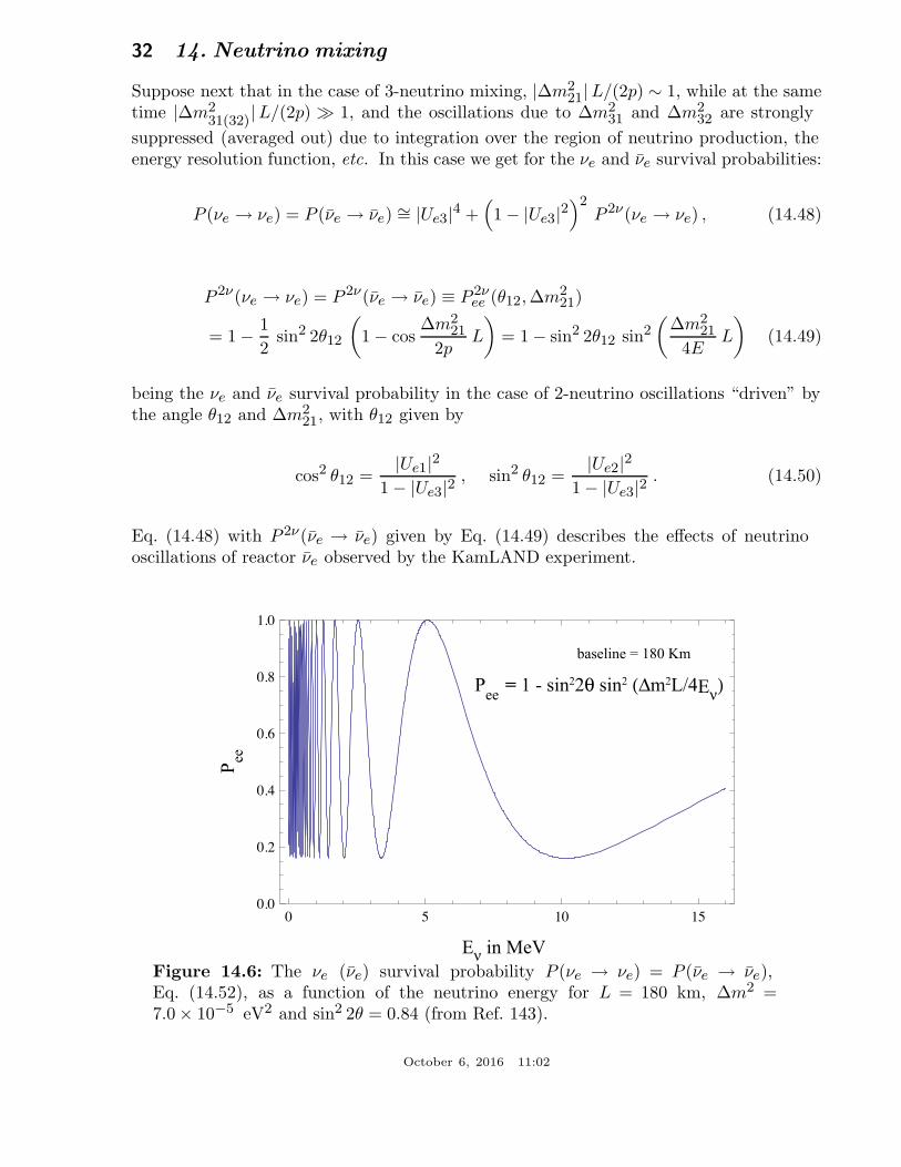
32 14. Neutrino mixing
Suppose next that in the case of 3-neutrino mixing, |∆m221|L/(2p) ∼ 1, while at the same
time |∆m231(32)
|L/(2p) ≫ 1, and the oscillations due to ∆m231 and ∆m2
32 are strongly
suppressed (averaged out) due to integration over the region of neutrino production, theenergy resolution function, etc. In this case we get for the νe and νe survival probabilities:
P (νe → νe) = P (νe → νe) ∼= |Ue3|4 +(
1 − |Ue3|2)2
P 2ν(νe → νe) , (14.48)
P 2ν(νe → νe) = P 2ν(νe → νe) ≡ P 2νee (θ12, ∆m2
21)
= 1 − 1
2sin2 2θ12
(
1 − cos∆m2
21
2pL
)
= 1 − sin2 2θ12 sin2(
∆m221
4EL
)
(14.49)
being the νe and νe survival probability in the case of 2-neutrino oscillations “driven” bythe angle θ12 and ∆m2
21, with θ12 given by
cos2 θ12 =|Ue1|2
1 − |Ue3|2, sin2 θ12 =
|Ue2|21 − |Ue3|2
. (14.50)
Eq. (14.48) with P 2ν(νe → νe) given by Eq. (14.49) describes the effects of neutrinooscillations of reactor νe observed by the KamLAND experiment.
Eν in MeV
Pee
= 1 - sin22θ sin2 (∆m2L/4Eν)
baseline = 180 Km
Pee
0 5 10 15
0.0
0.2
0.4
0.6
0.8
1.0
Figure 14.6: The νe (νe) survival probability P (νe → νe) = P (νe → νe),Eq. (14.52), as a function of the neutrino energy for L = 180 km, ∆m2 =7.0 × 10⁻⁵ eV2 and sin2 2θ = 0.84 (from Ref. 143).
October 6, 2016 11:02
14. Neutrino mixing 33
The data of ν-oscillations experiments were often analyzed in the past, and in certaincases new data are still analyzed at present, assuming 2-neutrino mixing:
|νl〉 = |ν1〉 cos θ + |ν2〉 sin θ , |νx〉 = −|ν1〉 sin θ + |ν2〉 cos θ , (14.51)
where θ is the neutrino mixing angle in vacuum and νx is another flavour neutrino orsterile (anti-) neutrino, x = l′ 6= l or νx ≡ νsL. In this case we have [139]:
P 2ν(νl → νl) = 1 − 1
2sin2 2θ
(
1 − cos 2πL
Lv
)
= 1 − sin2 2θ
(
sin2 ∆m2
4EL
)
,
P 2ν(νl → νx) = 1 − P 2ν(νl → νl) , (14.52)
where Lv = 4π E/∆m2 (p = E), ∆m2 = m22 − m2
1 > 0. Combining the CPT invarianceconstraints with the probability conservation one obtains: P (νl → νx) = P (νl → νx) =P (νx → νl) = P (νx → νl). These equalities and Eq. (14.52) with l = µ and x = τ wereused, for instance, in the analysis of the Super-K atmospheric neutrino data [17], in whichthe first compelling evidence for oscillations of neutrinos was obtained. The probabilityP 2ν(νl → νx), Eq. (14.52), depends on two factors: on (1 − cos 2πL/Lv), which exhibitsoscillatory dependence on the distance L and on the neutrino energy p = E (hence thename “neutrino oscillations”), and on sin2 2θ, which determines the amplitude of theoscillations. In order to have P 2ν(νl → νx) ∼= 1, two conditions have to be fulfilled:one should have sin2 2θ ∼= 1 and Lv . 2πL with cos 2πL/Lv ∼= −1. If Lv ≫ 2πL, theoscillations do not have enough time to develop on the way to the neutrino detectorand P (νl → νx) ∼= 0, while P (νl → νl) ∼= 1. The preceding comments are illustrated inFig. 14.6 showing the dependence of the probability P 2ν(νe → νe) = P 2ν(νe → νe) on theneutrino energy.
Table 14.4: Sensitivity of different oscillation experiments.
Source Type of ν E[MeV] L[km] min(∆m2)[eV2]
Reactor νe ∼ 1 1 ∼ 10−3
Reactor νe ∼ 1 100 ∼ 10−5
Accelerator νµ, νµ ∼ 103 1 ∼ 1
Accelerator νµ, νµ ∼ 103 1000 ∼ 10−3
Atmospheric ν’s νµ,e, νµ,e ∼ 103 104 ∼ 10−4
Sun νe ∼ 1 1.5 × 10⁸ ∼ 10−11
A given experiment searching for neutrino oscillations is specified, in particular,by the average energy of the neutrinos being studied, E, and by the source-detectordistance L. The requirement Lv
jk . 2πL determines the minimal value of a generic
neutrino mass squared difference ∆m2 > 0, to which the experiment is sensitive (figure
October 6, 2016 11:02
34 14. Neutrino mixing
of merit of the experiment): min(∆m2) ∼ 2E/L. Because of the interference nature ofneutrino oscillations, experiments can probe, in general, rather small values of ∆m2
(see, e.g., Ref. 135). Values of min(∆m2), characterizing qualitatively the sensitivity ofdifferent experiments are given in Table 14.4. They correspond to the reactor experimentsChooz, Daya Bay, RENO, Double Chooz (L ∼ 1 km) and KamLAND (L ∼ 100 km),to accelerator experiments - past (L ∼ 1 km), and current (K2K, MINOS, OPERA,T2K, NOνA [115]) , L ∼ (300 ÷ 1000) km), to the Super-Kamiokande, MINOS andIceCube-DeepCore experiments studying atmospheric neutrino oscillations, and to thesolar neutrino experiments.
14.8. Matter effects in neutrino oscillations
The presence of matter can change drastically the pattern of neutrino oscillations:neutrinos can interact with the particles forming the matter. Accordingly, the Hamiltonianof the neutrino system in matter Hm, differs from the Hamiltonian in vacuum H0,Hm = H0 + Hint, where Hint describes the interaction of neutrinos with the particles ofmatter. When, for instance, νe and νµ propagate in matter, they can scatter (due to Hint)on the electrons (e−), protons (p) and neutrons (n) present in matter. The incoherentelastic and the quasi-elastic scattering, in which the states of the initial particles changein the process (destroying the coherence between the neutrino states), are not of interest- they have a negligible effect on the solar neutrino propagation in the Sun and on thesolar, atmospheric and reactor neutrino propagation in the Earth [144]: even in thecenter of the Sun, where the matter density is relatively high (∼ 150 g/cm3), a νe withenergy of 1 MeV has a mean free path with respect to the indicated scattering processes∼ 1010 km. We recall that the solar radius is much smaller: R⊙ = 6.96 × 10⁵ km. Theoscillating νe and νµ can scatter also elastically in the forward direction on the e−, p andn, with the momenta and the spin states of the particles remaining unchanged. In such aprocess the coherence of the neutrino states is preserved.
The νe and νµ coherent elastic scattering on the particles of matter generatesnontrivial indices of refraction of the νe and νµ in matter [26]: κ(νe) 6= 1, κ(νµ) 6= 1.Most importantly, we have κ(νe) 6= κ(νµ). The difference κ(νe) − κ(νµ) is determinedessentially by the difference of the real parts of the forward νe − e− and νµ − e−
elastic scattering amplitudes [26] Re [Fνe−e−(0)] − Re [Fνµ−e−(0)]: due to the flavour
symmetry of the neutrino – quark (neutrino – nucleon) neutral current interaction, theforward νe − p, n and νµ − p, n elastic scattering amplitudes are equal and therefore donot contribute to the difference of interest [145]. The imaginary parts of the forwardscattering amplitudes (responsible, in particular, for decoherence effects) are proportionalto the corresponding total scattering cross-sections and in the case of interest arenegligible in comparison with the real parts. The real parts of the amplitudes Fνe−e−(0)and Fνµ−e−(0) can be calculated in the Standard Model. To leading order in the Fermi
constant GF , only the term in Fνe−e−(0) due to the diagram with exchange of a virtual
W±-boson contributes to Fνe−e−(0) − Fνµ−e−(0). One finds the following result for
October 6, 2016 11:02
14. Neutrino mixing 35
κ(νe) − κ(νµ) in the rest frame of the scatters [26,146,147]:
κ(νe) − κ(νµ) =2π
p2
(
Re [Fνe−e−(0)] − Re [Fνµ−e−(0)])
= − 1
p
√2GF Ne , (14.53)
where Ne is the electron number density in matter. Given κ(νe) − κ(νµ), the system ofevolution equations describing the νe ↔ νµ oscillations in matter reads [26]:
id
dt
(
Ae(t, t0)Aµ(t, t0)
)
=
(
−ǫ(t) ǫ′
ǫ′ ǫ(t)
)(
Ae(t, t0)Aµ(t, t0)
)
(14.54)
where Ae(t, t0) (Aµ(t, t0)) is the amplitude of the probability to find νe (νµ) at time t ofthe evolution of the system if at time t0 ≤ t the neutrino νe or νµ has been produced and
ǫ(t) =1
2[
∆m2
2Ecos 2θ −
√2GF Ne(t)], ǫ′ =
∆m2
4Esin 2θ. (14.55)
The term√
2GF Ne(t) in ǫ(t) accounts for the effects of matter on neutrino oscillations.The system of evolution equations describing the oscillations of antineutrinos νe ↔ νµ inmatter has exactly the same form except for the matter term in ǫ(t) which changes sign.The effect of matter in neutrino oscillations is usually called the Mikheyev, Smirnov,Wolfenstein (or MSW) effect.
Consider first the case of νe ↔ νµ oscillations in matter with constant density:Ne(t) = Ne = const. Due to the interaction term Hint in Hm, the eigenstates of theHamiltonian of the neutrino system in vacuum, |ν1,2〉 are not eigenstates of Hm. Forthe eigenstates |νm
1,2〉 of Hm, which diagonalize the evolution matrix in the r.h.s. of the
system Eq. (14.54) we have:
|νe〉 = |νm1 〉 cos θm + |νm
2 〉 sin θm , |νµ〉 = −|νm1 〉 sin θm + |νm
2 〉 cos θm . (14.56)
Here θm is the neutrino mixing angle in matter [26],
sin 2θm =tan2θ
√
(1 − NeNres
e)2 + tan2 2θ
, cos 2θm =1 − Ne/N
rese
√
(1 − NeNres
e)2 + tan2 2θ
, (14.57)
where the quantity
Nrese =
∆m2 cos 2θ
2E√
2GF
∼= 6.56 × 10⁶ ∆m2[eV2]
E[MeV]cos 2θ cm−3 NA , (14.58)
is called (for ∆m2 cos 2θ > 0) “resonance density” [27,146], NA being Avogadro’s number.The “adiabatic” states |νm
1,2〉 have energies Em1,2 whose difference is given by
Em2 − Em
1 =∆m2
2E
(
(1 − Ne
Nrese
)2 cos2 2θ + sin2 2θ
)12≡ ∆M2
2E. (14.59)
October 6, 2016 11:02
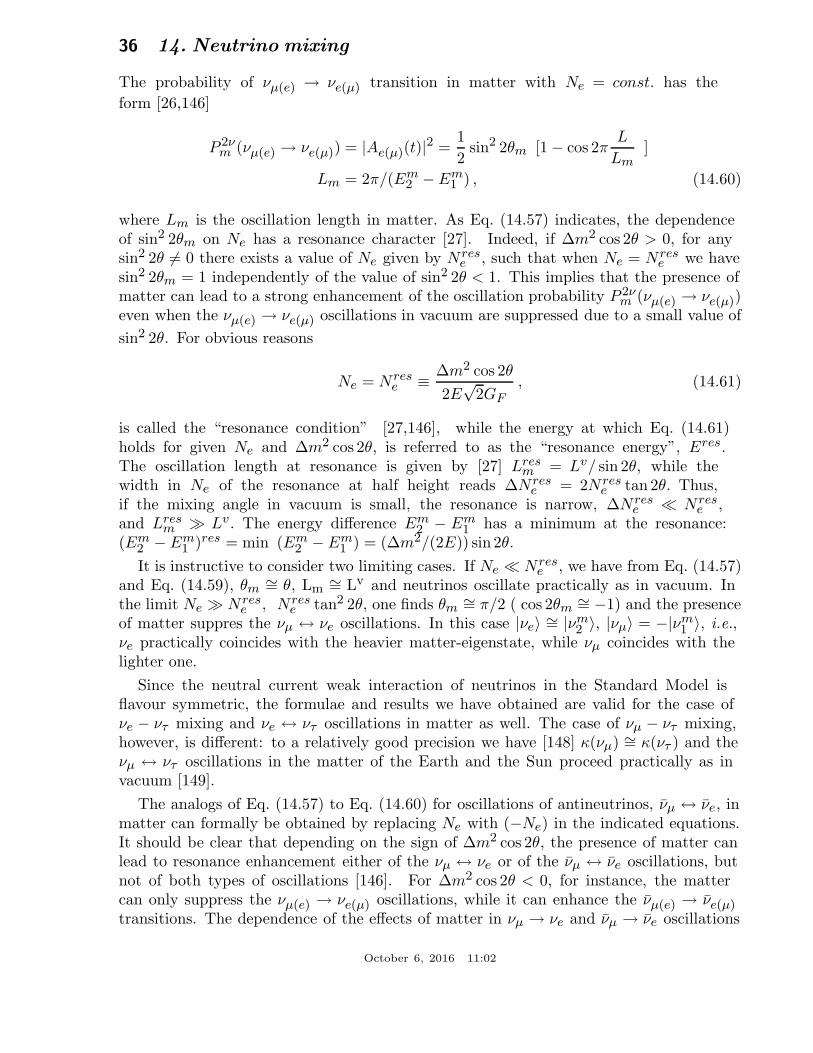
36 14. Neutrino mixing
The probability of νµ(e) → νe(µ) transition in matter with Ne = const. has the
form [26,146]
P 2νm (νµ(e) → νe(µ)) = |Ae(µ)(t)|2 =
1
2sin2 2θm [1 − cos 2π
L
Lm]
Lm = 2π/(Em2 − Em
1 ) , (14.60)
where Lm is the oscillation length in matter. As Eq. (14.57) indicates, the dependenceof sin2 2θm on Ne has a resonance character [27]. Indeed, if ∆m2 cos 2θ > 0, for anysin2 2θ 6= 0 there exists a value of Ne given by Nres
e , such that when Ne = Nrese we have
sin2 2θm = 1 independently of the value of sin2 2θ < 1. This implies that the presence ofmatter can lead to a strong enhancement of the oscillation probability P 2ν
m (νµ(e) → νe(µ))even when the νµ(e) → νe(µ) oscillations in vacuum are suppressed due to a small value of
sin2 2θ. For obvious reasons
Ne = Nrese ≡ ∆m2 cos 2θ
2E√
2GF, (14.61)
is called the “resonance condition” [27,146], while the energy at which Eq. (14.61)holds for given Ne and ∆m2 cos 2θ, is referred to as the “resonance energy”, Eres.The oscillation length at resonance is given by [27] Lres
m = Lv/ sin 2θ, while thewidth in Ne of the resonance at half height reads ∆Nres
e = 2Nrese tan 2θ. Thus,
if the mixing angle in vacuum is small, the resonance is narrow, ∆Nrese ≪ Nres
e ,and Lres
m ≫ Lv. The energy difference Em2 − Em
1 has a minimum at the resonance:(Em
2 − Em1 )res = min (Em
2 − Em1 ) = (∆m2/(2E)) sin 2θ.
It is instructive to consider two limiting cases. If Ne ≪ Nrese , we have from Eq. (14.57)
and Eq. (14.59), θm∼= θ, Lm
∼= Lv and neutrinos oscillate practically as in vacuum. Inthe limit Ne ≫ Nres
e , Nrese tan2 2θ, one finds θm
∼= π/2 ( cos 2θm∼= −1) and the presence
of matter suppres the νµ ↔ νe oscillations. In this case |νe〉 ∼= |νm2 〉, |νµ〉 = −|νm
1 〉, i.e.,νe practically coincides with the heavier matter-eigenstate, while νµ coincides with thelighter one.
Since the neutral current weak interaction of neutrinos in the Standard Model isflavour symmetric, the formulae and results we have obtained are valid for the case ofνe − ντ mixing and νe ↔ ντ oscillations in matter as well. The case of νµ − ντ mixing,however, is different: to a relatively good precision we have [148] κ(νµ) ∼= κ(ντ ) and theνµ ↔ ντ oscillations in the matter of the Earth and the Sun proceed practically as invacuum [149].
The analogs of Eq. (14.57) to Eq. (14.60) for oscillations of antineutrinos, νµ ↔ νe, inmatter can formally be obtained by replacing Ne with (−Ne) in the indicated equations.It should be clear that depending on the sign of ∆m2 cos 2θ, the presence of matter canlead to resonance enhancement either of the νµ ↔ νe or of the νµ ↔ νe oscillations, butnot of both types of oscillations [146]. For ∆m2 cos 2θ < 0, for instance, the mattercan only suppress the νµ(e) → νe(µ) oscillations, while it can enhance the νµ(e) → νe(µ)transitions. The dependence of the effects of matter in νµ → νe and νµ → νe oscillations
October 6, 2016 11:02
14. Neutrino mixing 37
on sgn(∆m2 cos 2θ) is at basis of the plans to determine the sign of ∆m231(32)
, and thus
the type of spectrum neutrino masses obey - with normal or inverted ordering - in longbaseline neutrino oscillation experiments (NOνA, DUNE) and in atmospheric neutrinoexperiments with large volume detectors (PINGU, ORCA, INO, Hyper-Kamiokande,DUNE).
The discussed disparity between the behavior of neutrinos and that of antineutrinosis a consequence of the fact that the matter in the Sun or in the Earth we areinterested in is not charge-symmetric (it contains e−, p and n, but does not containtheir antiparticles) and therefore the oscillations in matter are neither CP- nor CPT-invariant [65]. Thus, even in the case of 2-neutrino mixing and oscillations we have, e.g.,P 2ν
m (νµ → νe) 6= P 2νm (νµ → νe) and P 2ν
m (νe → νµ(τ)) 6= P 2νm (νe → νµ(τ)).
The νµ ↔ νe (νµ ↔ νe) and νe ↔ νµ(τ) (νe ↔ νµ(τ)) oscillations in matter will beinvariant with respect to the operation of time reversal if the Ne distribution along theneutrino path is symmetric with respect to this operation [63,150]. The latter conditionis fulfilled (to a good approximation) for the Ne distribution along a path of a neutrinocrossing the Earth [151].
14.8.1. Effects of Earth matter on oscillations of neutrinos. Analytic expres-
sions for oscillation probabilities :
The formalism we have developed can be applied, e.g., to the study of matter effectsin the νe ↔ νµ(τ) (νµ(τ) ↔ νe) and νe ↔ νµ(τ) (νµ(τ) ↔ νe) oscillations of neutrinos
which traverse the Earth [152]. Indeed, the Earth density distribution in the existingEarth models [151] is assumed to be spherically symmetric and there are two majordensity structures - the core and the mantle, and a certain number of substructures(shells or layers). The Earth radius is R⊕ = 6371 km; the Earth core has a radius ofRc = 3486 km, so the Earth mantle depth is 2885 km. For a spherically symmetricEarth density distribution, the neutrino trajectory in the Earth is specified by the valueof the nadir angle θn of the trajectory. For θn ≤ 33.17o, or path lengths L ≥ 10660km, neutrinos cross the Earth core. The path length for neutrinos which cross onlythe Earth mantle is given by L = 2R⊕ cos θn. If neutrinos cross the Earth core, thelengths of the paths in the mantle, 2Lman, and in the core, Lcore, are determined by:
Lman = R⊕ cos θn − (R2c −R2
⊕ sin2 θn)12 , Lcore = 2(R2
c −R2⊕ sin2 θn)
12 . The mean electron
number densities in the mantle and in the core according to the PREM model read [151]:Nman
e∼= 2.2 cm−3 NA, N c
e∼= 5.4 cm−3 NA. Thus, we have N c
e∼= 2.5 Nman
e . Thechange of Ne from the mantle to the core can well be approximated by a stepfunction [151]. The electron number density Ne changes relatively little around theindicated mean values along the trajectories of neutrinos which cross a substantial partof the Earth mantle, or the mantle and the core, and the two-layer constant densityapproximation, Nman
e = const. = Nmane , Nc
e = const. = Nce , Nman
e and Nce being the
mean densities along the given neutrino path in the Earth, was shown to be sufficientlyaccurate in what concerns the calculation of neutrino oscillation probabilities [63,154,155](and references quoted in [154,155]) in a large number of specific cases. This is relatedto the fact that the relatively small changes of density along the path of the neutrinos inthe mantle (or in the core) take place over path lengths which are typically considerably
October 6, 2016 11:02
38 14. Neutrino mixing
smaller than the corresponding oscillation length in matter.
In the case of 3-neutrino mixing and for neutrino energies of E & 2 GeV, theeffects due to ∆m2
21 (|∆m221| ≪ |∆m2
31(23)|, see Eq. (14.43)) in the neutrino oscillation
probabilities are sub-dominant and to leading order can be neglected: the correspondingresonance density |Nres
e21 |. 0.25 cm−3 NA ≪ Nman,ce and the Earth matter strongly
suppresses the oscillations due to ∆m221. For oscillations in vacuum this approximation
is valid in the case of NO (IO) neutrino mass spectrum (see Section 2) as long as theleading order contribution due to ∆m2
31(23) in the relevant probabilities is bigger than
approximately 10−3. In this case the 3-neutrino νe → νµ(τ) (νe → νµ(τ)) and νµ(τ) → νe
(νµ(τ) → νe) transition probabilities for neutrinos traversing the Earth, reduce effectively
to a 2-neutrino transition probability (see, e.g., Refs. [155–157]) , with ∆m231(23)
and
θ13 playing the role of the relevant 2-neutrino vacuum oscillation parameters. We notethat in the approximation of negligible ∆m2
21 we have ∆m231 = ∆m2
32. Therefore in whatfollows in this part of the article we will use, whenever relevant, only ∆m2
31 in the analyticexpressions.
As we have discussed in Sections 14.2 and will be discussed in greater detail inSection 14.12, the value of sin2 2θ13 has been determined with a rather high precisionin the Daya Bay [38] and RENO [39] experiments. The best fit values found in the twoexperiments read, respectively, sin2 2θ13 = 0.084 [38] and 0.087 [39]. The 3-neutrinooscillation probabilities of the atmospheric and accelerator νe,µ having energy E & 2 GeVand crossing the Earth along a trajectory characterized by a nadir angle θn, for instance,have the following form in the approximation of negligible ∆m2
21:
P 3νm (νe → νe) ∼= 1 − P 2ν
m , (14.62)
P 3νm (νe → νµ) ∼= P 3ν
m (νµ → νe) ∼= s223 P 2ν
m , P 3νm (νe → ντ ) ∼= c223 P 2ν
m , (14.63)
P 3νm (νµ → νµ) ∼= 1 − s4
23 P 2νm − 2c223s
223
[
1 − Re (e−iκA2νm (ν′ → ν′))
]
, (14.64)
P 3νm (νµ → ντ ) = 1 − P 3ν
m (νµ → νµ) − P 3νm (νµ → νe). (14.65)
Here P 2νm ≡ P 2ν
m (∆m231, θ13; E, θn) is the probability of the 2-neutrino νe → ν′ ≡
(s23νµ + c23ντ ) oscillations in the Earth, and κ and A2νm (ν′ → ν′) ≡ A2ν
m are known phaseand 2-neutrino transition probability amplitude (see, e.g., Refs. [155,156]) . We notethat Eq. (14.62) to Eq. (14.64) are based only on the assumptions that |Nres
e21 | is muchsmaller than the densities in the Earth mantle and core and that |∆m2
21| ≪ |∆m231(23)|,
and does not rely on the constant density approximation. Similar results are validfor the corresponding antineutrino oscillation probabilities: one has just to replaceP 2ν
m , κ and A2νm in the expressions given above with the corresponding quantities for
antineutrinos (the latter are obtained from those for neutrinos by changing the signin front of Ne). Obviously, we have: P (νe(µ) → νµ(e)), P (νe(µ) → νµ(e)) ≤ sin2 θ23,
and P (νe → ντ ), P (νe → ντ ) ≤ cos2 θ23. The one ∆m2 dominance approximationand correspondingly Eq. (14.62) to Eq. (14.65) were used by the Super-Kamiokande
October 6, 2016 11:02
14. Neutrino mixing 39
Collaboration in their 2006 neutrino oscillation analysis of the multi-GeV atmosphericneutrino data [158].
In the case of neutrinos crossing only the Earth mantle and in the constant densityapproximation, P 2ν
m is given by the r.h.s. of Eq. (14.60) with θ, ∆m2 and Ne replacedrespectively by θ13, ∆m2
31 and Nmane (corresponding to the given θn) in the relevant
expressions Eq. (14.57), Eq. (14.58) and Eq. (14.59) for sin 2θm, Nrese and (Em
2 − Em1 ),
while for κ and A2νm we have (see, e.g., Ref. 155):
κ ∼= 1
2[∆m2
31
2EL +
√2GF Nman
e L − ∆M231L
2E],
A2νm = 1 + (e−i
∆M231L
2E − 1) cos2 θm13 , (14.66)
where ∆M231 and θm
13 can be obtained from Eq. (14.59) and Eq. (14.57) by setting θ = θ13,
∆m2 = ∆m231 > 0, Nres
e = Nrese31 = ∆m2
31 cos 2θ13/(2E√
2GF ) and Ne = Nmane (θn).
Clearly, θm13 is the mixing angle in the mantle which coincides in vacuum with θ13. In the
expressions for P 2νm ≡ P 2ν
m (∆m231, θ13; E, θn, Nman
e ), κ and A2νm in the case of oscillations
in the mantle, L = 2R⊕ cos θn is the distance the neutrino travels in the mantle. Thecorresponding expressions for antineutrino oscillations, as we have noticed earlier, can beobtained from those derived above by making the change Nman
e → − Nmane .
The analytic results for P 2νm (∆m2
31, θ13; E, θn, Nmane ), κ and A2ν
m , described above andobtained in the constant mantle density approximation, as we have already remarked,provide a relatively precise description of the νµ(e) → νe(µ), νe → νe(τ), etc. oscillationprobabilities in the Earth mantle if for each given trajectory of the neutrinos in themantle, specified by the nadir angle θn, in the calculations one uses for Nman
e the meanvalue of the electron number density along that specific trajectory: Nman
e = Nmane (θn),
where Nmane (θn) should be calculated using the density distribution given by the existing
Earth models [151].
It follows from Eq. (14.62) and Eq. (14.63) that for ∆m231 cos 2θ13 > 0, the
oscillation effects of interest, e.g., in the νe(µ) → νµ(e) and νe → ντ transitions will
be maximal if P 2νm
∼= 1, i.e., if Eq. (14.61) leading to sin2 2θm∼= 1 is fulfilled, and ii)
cos(∆M2L/(2E)) ∼= −1. Given the value of Nmane , the first condition determines the
neutrino’s energy, while the second determines the path length L, for which one can haveP 2ν
m∼= 1. For ∆m2
31∼= 2.5 × 10⁻³ eV2, sin2 2θ13
∼= 0.090 and Nmane
∼= 2.2 NAcm−3, onefinds that Eres
∼= 7.1 GeV and L ∼= 3522/ sin 2θ13 km ∼= 11740 km. Since for neutrinoscrossing only the mantle L . 10660 km, the second condition can be satisfied only ifsin2 2θ13 & 0.11, which falls marginally in the 3σ range of the experimentally allowed valuesof sin2 2θ13. We still get a significant amplification of the probability P 2ν
m , and thereforeof P (νe(µ) → νµ(e)) and P (νe → ντ ), even when cos(∆M2L/(2E)) = −0.5(−0.2): in this
case P 2νm
∼= 0.75 (0.60). For sin2 2θ13∼= 0.090 we have cos(∆M2L/(2E)) = −0.5(−0.2) if
L ∼= 7826 (6622) km. Thus, for ∆m231 > 0, the Earth matter effects can amplify P 2ν
m ,and therefore P (νe(µ) → νµ(e)) and P (νe → ντ ), significantly when the neutrinos crossonly the mantle, for E ∼ 7 GeV and sufficiently large path lengths L.
If ∆m231 < 0 the same considerations apply for the corresponding antineutrino
oscillation probabilities P 2νm = P 2ν
m (νe → (s23νµ + c23ντ )) and correspondingly for
October 6, 2016 11:02
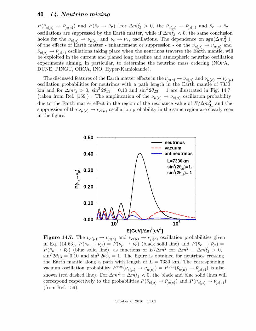
40 14. Neutrino mixing
P (νe(µ) → νµ(e)) and P (νe → ντ ). For ∆m231 > 0, the νe(µ) → νµ(e) and νe → ντ
oscillations are suppressed by the Earth matter, while if ∆m231 < 0, the same conclusion
holds for the νe(µ) → νµ(e) and νe → ντ , oscillations. The dependence on sgn(∆m231)
of the effects of Earth matter - enhancement or suppression - on the νe(µ) → νµ(e) andνe(µ) → νµ(e) oscillations taking place when the neutrinos traverse the Earth mantle, willbe exploited in the current and planed long baseline and atmospheric neutrino oscillationexperiments aiming, in particular, to determine the neutrino mass ordering (NOνA,DUNE, PINGU, ORCA, INO, Hyper-Kamiokande).
The discussed features of the Earth matter effects in the νµ(e) → νe(µ) and νµ(e) → νe(µ)oscillation probabilities for neutrinos with a path length in the Earth mantle of 7330km and for ∆m2
31 > 0, sin2 2θ13 = 0.10 and sin2 2θ23 = 1 are illustrated in Fig. 14.7(taken from Ref. [159]) . The amplification of the νµ(e) → νe(µ) oscillation probability
due to the Earth matter effect in the region of the resonance value of E/∆m231 and the
suppression of the νµ(e) → νe(µ) oscillation probability in the same region are clearly seenin the figure.
103
104
E[GeV]/∆m2[eV2]
0.00
0.10
0.20
0.30
0.40
0.50
P(ν
e→ν µ)
neutrinosvacuumantineutrinos
L=7330kmsin
2(2θ23)=1.
sin2(2θ13)=.1
Figure 14.7: The νe(µ) → νµ(e) and νe(µ) → νµ(e) oscillation probabilities given
in Eq. (14.63), P (νe → νµ) = P (νµ → νe) (black solid line) and P (νe → νµ) =P (νµ → νe) (blue solid line), as functions of E/∆m2 for ∆m2 ≡ ∆m2
31 > 0,sin2 2θ13 = 0.10 and sin2 2θ23 = 1. The figure is obtained for neutrinos crossingthe Earth mantle along a path with length of L = 7330 km. The correspondingvacuum oscillation probability P vac(νe(µ) → νµ(e)) = P vac(νe(µ) → νµ(e)) is also
shown (red dashed line). For ∆m2 ≡ ∆m231 < 0, the black and blue solid lines will
correspond respectively to the probabilities P (νe(µ) → νµ(e)) and P (νe(µ) → νµ(e))
(from Ref. 159).
October 6, 2016 11:02
14. Neutrino mixing 41
In the case of neutrinos crossing the Earth core, new resonance-like effects becomepossible in the νµ → νe and νe → νµ(τ) (or νµ → νe and νe → νµ(τ)) transitions
[154–156,160–162]. For ∆m231 > 0 and certain values of sin2 θ13 . 0.05 we can have [161]
P 2νm (∆m2
31, θ13) ∼= 1, and correspondingly maximal P 3νm (νe → νµ) = P 3ν
m (νµ → νe) ∼= s223,
only due to the effect of maximal constructive interference between the amplitudes ofthe νe → ν′ transitions in the Earth mantle and in the Earth core. The effect differsfrom the MSW one and the enhancement happens in the case of interest at a valueof the energy between the MSW resonance energies corresponding to the density inthe mantle and that of the core, or at a value of the resonance density Nres
e whichlies between the values of Ne in the mantle and in the core [154]. In Refs. [154,155]the enhancement was called “neutrino oscillation length resonance (NOLR)”, while inRefs. [156,160] the term “parametric resonance” for the same effect was used [163].The mantle-core enhancement effect (or NOLR) is caused by the existence (for a givenneutrino trajectory through the Earth core) of points of resonance-like maximal neutrinoconversion, P 2ν
m (∆m231, θ13) = 1, in the corresponding space of neutrino oscillation
parameters [161]. For ∆m231 < 0 the mantle-core enhancement can take place for the
antineutrino transitions, νµ → νe and νe → νµ(τ). For neutrinos crossing the Earth core,
analytic expressions for P 2νm (∆m2
31, θ13) and κ, A2νm were derived in the two-layer constant
density approximation for the Earth density distribution in [154] and [155], respectively.
A rather complete set of values of ∆m231/E > 0 and sin2 2θ13 for which
P 2νm (∆m2
31, θ13) = 1 was found in Ref. 161. In the two-layer constant density ap-proximation, the values of ∆m2
31/E > 0 and sin2 2θ13 at which P 2νm (∆m2
31, θ13) = 1 canbe derived as solutions of the following system of equations [161]:
tanφman = ±√
− cos 2θcore13
cos(2θcore13 − 4θman
13 ), (14.67)
tan φcore = ± cos 2θman13
√
− cos(2θcore13 ) cos(2θcore
13 − 4θman13 )
, (14.68)
where the signs in the two equations are correlated, 2φman = (Em3 − Em
1 )manLman,2φcore = (Em
3 − Em1 )coreLcore, 2Lman and Lcore are the neutrino path lengths in the
Earth mantle and the core, and θman13 and θcore
13 are the values of the angle θ13 inthe mantle and in the core. The expressions for (Em
3 − Em1 )man ((Em
3 − Em1 )core) and
θman13 (θcore
13 ) can be obtained respectively from Eq. (14.59) and Eq. (14.57) by setting
θ = θ13, ∆m2 = ∆m231, Nres
e = Nrese31 = ∆m2
31 cos 2θ13/(2E√
2GF ) and Ne = Nmane (θn)
(Ne = N coree (θn)).
The location of the points where P 2νm (∆m2
31, θ13) = 1 in the ∆m231/E − sin2 2θ13 plane
determines the regions in the plane where P 2νm (∆m2
31, θ13) is large, P 2νm (∆m2
31, θ13) & 0.5.These regions vary slowly with the nadir angle, being remarkably wide in the nadirangle and rather wide in the neutrino energy [161], so that the transitions of interestcan produce noticeable effects in the measured observables. For sin2 θ13 . 0.05, thereare two sets of values of (∆m2
31/E, sin2 θ13) for which P 2νm (∆m2
31, θ13) = 1, and thustwo regions in ∆m2
31/E − sin2 2θ13 plane where P 2νm (∆m2
31, θ13) & 0.5. For ∆m231 =
October 6, 2016 11:02
42 14. Neutrino mixing
2.5 × 10⁻³ eV2 and nadir angle, e.g., θn=0 (Earth center crossing neutrinos), we haveP 2ν
m (∆m231, θ13) = 1 at (E, sin2 2θ13) =(3.4 GeV,0.034) and (5.2 GeV,0.15). At the same
time for E =3.4 GeV (5.2 Gev), the probability P 2νm (∆m2
31, θ13) & 0.5 for the values ofsin2 2θ13 from the interval 0.02 . sin2 2θ13 . 0.10 (0.04 . sin2 2θ13 . 0.26). Similar resultshold for neutrinos crossing the Earth core along the trajectories with θn 6= 0 (for furtherdetails see the last article in Ref. 161; see also the last article in Ref. 162).
The mantle-core enhancement of P 2νm (or P 2ν
m ) is relevant, in particular, for thesearches of sub-dominant νe(µ) → νµ(e) (or νe(µ) → νµ(e)) oscillations of atmosphericneutrinos having energies E & 2 GeV and crossing the Earth core on the way to thedetector (see Ref. 154 to Ref. 162 and the references quoted therein).
The effects of Earth matter on the oscillations of atmospheric and acceleratorneutrinos have not been observed so far. At present there are no compelling evidences foroscillations of the atmospheric νe and/or νe.
In the case of oscillations of atmospheric neutrinos in the Earth one has to take intoaccount also the following considerations. The fluxes of atmospheric νe,µ of energy E,which reach the detector after crossing the Earth along a given trajectory specified bythe value of θn, Φνe,µ(E, θn), are given by the following expressions in the case of the3-neutrino oscillations under discussion [155,156]:
Φνe(E, θn) ∼= Φ0νe
(
1 + [s223r − 1] P 2ν
m
)
, (14.69)
Φνµ(E, θn) ∼= Φ0νµ
(
1 + s423[(s
223 r)−1 − 1]P 2ν
m − 2c223s223
[
1 − Re (e−iκA2νm (ντ → ντ ))
])
,
(14.70)where Φ0
νe(µ)= Φ0
νe(µ)(E, θn) is the νe(µ) flux in the absence of neutrino oscillations and
r ≡ r(E, θn) ≡Φ0
νµ(E, θn)
Φ0νe
(E, θn). (14.71)
It follows from the global analyses of the neutrino oscillation data that the neutrinomixing parameter s2
23 lies (at 3σ CL) in the interval (0.38 - 0.64). For NO (IO) neutrinomass spectrum, the three groups which performed recent global analyses, obtained thefollowing best fit values of s2
23 (see Section 14.2): 0.452 (0.455) [52], 0.452 (0.579) [53]and 0.567 (0.573) [54], while in the latest analysis [60] the authors find 0.437 (0.569).For the predicted ratio r(E, θn) of the atmospheric νµ and νe fluxes for i) the Earthcore crossing and ii) only mantle crossing neutrinos, having trajectories for which0.3 . cos θn ≤ 1.0, one has [164] r(E, θn) ∼= (2.6 ÷ 4.5) for neutrinos giving the maincontribution to the multi-GeV samples, E ∼= (2÷ 10) GeV. Thus, for s2
23 = 0.5 (0.64) onefinds for the multi-GeV neutrinos: s4
23[1−(s223 r(E, θz))
−1] ∼= 0.06−0.14 (0.16−0.27) and(s2
23 r(E, θz) − 1) ∼= 0.3− 1.3 (0.66− 1.9). Thus, the impact of the possible enhancementof P 2ν
m∼= 1 would be largest for the flux of multi-GeV νe, Φνe(E, θn), traversing the
Earth. As the preceding discussion suggests and detailed calculations show (see the firsttwo articles quoted in Ref. 162), the sensitivity of the atmospheric neutrino experimentsto the neutrino mass ordering depends strongly on the chosen value of sin2 θ23 from
October 6, 2016 11:02
14. Neutrino mixing 43
its 3σ allowed range: it is maximal (minimal) for the maximal (minimal) allowed valueof sin2 θ23. In the case of the planned Hyper-Kamiokande detector and neutrino massspectrum with normal ordering, for instance, it is estimated [165] that for sin2 θ23 = 0.60it will take approximately (2-3) years to establish at 3σ CL that the spectrum is of theNO type, and approximately 10 years if sin2 θ23 = 0.40.
For water Cerenkov detectors, the charged current (CC) νl−N interaction cross sectionfor multi-GeV neutrinos is approximately by a factor of 2 bigger than the νl − N CCinteraction cross section. Since these detectors do not distinguish between the neutrinoand anti-neutrino induced CC events, determining that the neutrino mass spectrum iswith inverted ordering would require roughly by a factor of 2 longer period of dataacquisition than if the spectrum were with normal ordering.
The effects under discussion are larger, in general, for the multi-GeV neutrinos than forthe sub-GeV neutrinos having energies E ∼= (0.1 − 1.0) GeV. Indeed, for the sub-GeV νe
flux one finds in the limit of negligible θ13 [166]: Φνe(E, θn) ∼= Φ0νe
(1 + [c223r − 1]P 2νm ),
where P 2νm ≡ P 2ν
m (∆m221, θ12; E, θn) is the probability of the 2-neutrino oscillations
in the Earth due to ∆m221 and 2-neutrino mixing with angle θ12. For the neutrinos
giving contribution to the sub-GeV samples of Super-Kamiokande events one has [164]r(E, θz) ∼= 2.0. If s2
23 = 0.5 and r(E, θz) ∼= 2.0, we get (c223 r(E, θz) − 1) ∼= 0, andthe possible effects of the νµ → νe and νe → νµ(τ) transitions on the νe flux, andcorrespondingly in the sub-GeV e−like samples of events, would be rather stronglysuppressed independently of the values of the corresponding transition probabilities.
The same conclusions are valid for the effects of oscillations on the fluxes of, andevent rates due to, atmospheric antineutrinos νe and νµ. The formulae for anti-neutrinofluxes and oscillation probabilities are analogous to those for neutrinos (see, e.g., Refs.[155,156,162,166]) .
The expression for the probability of the νµ → νe oscillations taking place in the Earthmantle in the case of 3-neutrino mixing, in which both neutrino mass squared differences∆m2
21 and ∆m231 contribute and the CP violation effects due to the Dirac phase in the
neutrino mixing matrix are taken into account, has the following form in the constantdensity approximation and keeping terms up to second order in the two small parameters|α| ≡ |∆m2
21|/|∆m231| ≪ 1 and sin2 θ13 ≪ 1 [167]:
P 3ν manm (νµ → νe) ∼= P0 + Psin δ + Pcos δ + P3 . (14.72)
Here
P0 = sin2 θ23sin2 2θ13
(A − 1)2sin2[(A − 1)∆]
P3 = α2 cos2 θ23sin2 2θ12
A2sin2(A∆) , (14.73)
Psin δ = −α8 JCP
A(1 − A)(sin ∆) (sinA∆) (sin[(1 − A)∆]) , (14.74)
October 6, 2016 11:02
44 14. Neutrino mixing
Pcos δ = α8 JCP cot δ
A(1 − A)(cos∆) (sinA∆) (sin[(1 − A)∆]) , (14.75)
where
α =∆m2
21
∆m231
, ∆ =∆m2
31 L
4E, A =
√2GFNman
e2E
∆m231
, (14.76)
cot δ = J−1CP Re(Uµ3U
∗e3Ue2U
∗µ2) ∝ cos δ, and we recall that JCP = Im(Uµ3U
∗e3Ue2U
∗µ2).
The analytic expression for P 3ν manm (νµ → νe) given above is valid for [167] neutrino
path lengths in the mantle (L ≤ 10660 km) satisfying L . 10560 km E[GeV] (7.6 ×10⁻⁵ eV2/∆m2
21), and energies E & 0.34 GeV(∆m221/7.6×10−5 eV2) (1.4 cm−3NA/Nman
e ).The expression for the νµ → νe oscillation probability can be obtained formally fromthat for P 3ν man
m (νµ → νe) by making the changes A → −A and JCP → −JCP ,with JCP cot δ ≡ Re(Uµ3U
∗e3Ue2U
∗µ2) remaining unchanged. The term Psin δ in
P 3ν manm (νµ → νe) would be equal to zero if the Dirac phase in the neutrino
mixing matrix U possesses a CP-conserving value. Even in this case, however, we have
A(eµ) manCP ≡ (P 3ν man
m (νµ → νe) − P 3ν manm (νµ → νe)) 6= 0 due to the effects of the
Earth matter. It will be important to experimentally disentangle the effects of the Earth
matter and of JCP in A(eµ) manCP : this will allow to get information about the Dirac CP
violation phase in U . This can be done, in principle, by studying the energy dependenceof P 3ν man
m (νµ → νe) and P 3ν manm (νµ → νe). Since the sign of ∆m2
31(32) determines
for given L whether the probability P 3ν manm (νµ → νe) or P 3ν man
m (νµ → νe), as afunction of energy, can be resonantly enhanced or suppressed by the matter effects, thestudy of the energy dependence of P 3ν man
m (νµ → νe) and/or of P 3ν manm (νµ → νe) can
provide also information on sgn(∆m231(32)). In the vacuum limit of Nman
e = 0 (A = 0)
we have A(eµ) manCP = A
(eµ)CP (see Eq. (14.40)) and only the term Psin δ contributes to the
asymmetry A(eµ)CP .
The preceding remarks apply also to the probabilities P 3ν manm (νe → νµ) and
P 3ν manm (νe → νµ)). The probability P 3ν man
m (νe → νµ), for example, can formally beobtained from the expression for the probability P 3ν man
m (νµ → νe) by changing the signof the term Psin δ .
The expression for the probability P 3ν manm (νµ → νe) given in Eq. (14.72) and the
corresponding expression for P 3ν manm (νµ → νe) can be used for the interpretation of the
data of the current and the future planned long baseline oscillation experiments T2K,NOνA, MINOS+, DUNE [84] and T2HK [85].
October 6, 2016 11:02
14. Neutrino mixing 45
14.8.2. Oscillations of solar neutrinos :
14.8.2.1. Qualitative analysis:
Consider next the oscillations of solar νe while they propagate from the central partof the Sun, where they are produced, to the surface of the Sun [27,153] (see alsoRef. 26 and, e.g., Ref. 168). Details concerning the production, spectrum, magnitude andparticularities of the solar neutrino flux were discussed in Section 14.6, while the methodsof detection of solar neutrinos, description of solar neutrino experiments and of the datathey provided will be discussed in the next section (see also Ref. 169). The electronnumber density Ne changes considerably along the neutrino path in the Sun: it decreasesmonotonically from the value of ∼ 100 cm−3 NA in the center of the Sun to 0 at thesurface of the Sun. According to the contemporary solar models (see, e.g., Ref. [169,99]) ,Ne decreases approximately exponentially in the radial direction towards the surface ofthe Sun:
Ne(t) = Ne(t0) exp
{
− t − t0r0
}
, (14.77)
where (t − t0) ∼= d is the distance traveled by the neutrino in the Sun, Ne(t0) is theelectron number density at the point of νe production in the Sun, r0 is the scale-height ofthe change of Ne(t) and one has [169,99] r0 ∼ 0.1R⊙.
Consider the case of 2-neutrino mixing, Eq. (14.56). Obviously, if Ne changes with t (orequivalently with the distance) along the neutrino trajectory, the matter-eigenstates, theirenergies, the mixing angle and the oscillation length in matter, become, through theirdependence on Ne, also functions of t: |νm
1,2〉 = |νm1,2(t)〉, Em
1,2 = Em1,2(t), θm = θm(t) and
Lm = Lm(t). It is not difficult to understand qualitatively the possible behavior of theneutrino system when solar neutrinos propagate from the center to the surface of the Sunif one realizes that one is dealing effectively with a two-level system whose Hamiltoniandepends on time and admits “jumps” from one level to the other (see Eq. (14.54)).Consider the case of ∆m2 cos 2θ > 0. Let us assume first for simplicity that the electronnumber density at the point of a solar νe production in the Sun is much bigger than theresonance density, Ne(t0) ≫ Nres
e . Actually, this is one of the cases relevant to the solarneutrinos. In this case we have θm(t0) ∼= π/2 and the state of the electron neutrino in theinitial moment of the evolution of the system practically coincides with the heavier of thetwo matter-eigenstates:
|νe〉 ∼= |νm2 (t0)〉 . (14.78)
Thus, at t0 the neutrino system is in a state corresponding to the “level” with energyEm
2 (t0). When neutrinos propagate to the surface of the Sun they cross a layer ofmatter in which Ne = Nres
e : in this layer the difference between the energies of the two“levels” (Em
2 (t)−Em1 (t)) has a minimal value on the neutrino trajectory (Eq. (14.59) and
Eq. (14.61)). Correspondingly, the evolution of the neutrino system can proceed basicallyin two ways. First, the system can stay on the “level” with energy Em
2 (t), i.e., cancontinue to be in the state |νm
2 (t)〉 up to the final moment ts, when the neutrino reachesthe surface of the Sun. At the surface of the Sun Ne(ts) = 0 and therefore θm(ts) = θ,|νm
1,2(ts)〉 ≡ |ν1,2〉 and Em1,2(ts) = E1,2. Thus, in this case the state describing the neutrino
October 6, 2016 11:02
46 14. Neutrino mixing
system at t0 will evolve continuously into the state |ν2〉 at the surface of the Sun. UsingEq. (14.51) with l = e and x = µ, it is easy to obtain the probabilities to find νe and νµ
at the surface of the Sun:
P (νe → νe; ts, t0) ∼= |〈νe|ν2〉|2 = sin2 θ
P (νe → νµ; ts, t0) ∼= |〈νµ|ν2〉|2 = cos2 θ . (14.79)
It is clear that under the assumption made and if sin2 θ ≪ 1, practically a total νe → νµ
conversion is possible. This type of evolution of the neutrino system and the νe → νµ
transitions taking place during the evolution, are called [27] “adiabatic.” They arecharacterized by the fact that the probability of the “jump” from the upper “level”(having energy Em
2 (t)) to the lower “level” (with energy Em1 (t)), P ′, or equivalently the
probability of the νm2 (t0) → νm
1 (ts) transition, P ′ ≡ P ′(νm2 (t0) → νm
1 (ts)), on the wholeneutrino trajectory is negligible:
P ′ ≡ P ′(νm2 (t0) → νm
1 (ts)) ∼= 0 : adiabatic transitions . (14.80)
The second possibility is realized if in the resonance region, where the two “levels”approach each other most, the system “jumps” from the upper “level” to the lower “level”and after that continues to be in the state |νm
1 (t)〉 until the neutrino reaches the surfaceof the Sun. Evidently, now we have P ′ ≡ P ′(νm
2 (t0) → νm1 (ts)) ∼ 1. In this case the
neutrino system ends up in the state |νm1 (ts)〉 ≡ |ν1〉 at the surface of the Sun and
P (νe → νe; ts, t0) ∼= |〈νe|ν1〉|2 = cos2 θ
P (νe → νµ; ts, t0) ∼= |〈νµ|ν1〉|2 = sin2 θ . (14.81)
Obviously, if sin2 θ ≪ 1, practically no transitions of the solar νe into νµ will occur. Theconsidered regime of evolution of the neutrino system and the corresponding νe → νµ
transitions are usually referred to as “extremely nonadiabatic.”
Clearly, the value of the “jump” probability P ′ plays a crucial role in the the νe → νµ
transitions: it fixes the type of the transition and determines to a large extent theνe → νµ transition probability [153,170,171]. We have considered above two limitingcases. Obviously, there exists a whole spectrum of possibilities since P ′ can have anyvalue from 0 to cos2 θ [172,173]. In general, the transitions are called “nonadiabatic” ifP ′ is non-negligible.
Numerical studies have shown [27] that solar neutrinos can undergo both adiabatic andnonadiabatic νe → νµ transitions in the Sun and the matter effects can be substantial inthe solar neutrino oscillations for 10−8 eV2 .∆m2 . 10−4 eV2, 10−4 . sin2 2θ < 1.0.
The condition of adiabaticity of the solar νe transitions in Sun can be writtenas [153,170]
γ(t) ≡√
2GF(Nres
e )2
|Ne(t)|tan2 2θ
(
1 + tan−2 2θm(t))
32 ≫ 1
adiabatic transitions , (14.82)
October 6, 2016 11:02
14. Neutrino mixing 47
while if γ(t) .1 the transitions are nonadiabatic (see also Ref. 173), where Ne(t) ≡ddtNe(t). Condition in Eq. (14.82) implies that the νe → νµ(τ) transitions in the Sun will
be adiabatic if Ne(t) changes sufficiently slowly along the neutrino path. In order for thetransitions to be adiabatic, condition in Eq. (14.82) has to be fulfilled at any point of theneutrino’s path in the Sun.
14.8.2.2. The solar νe survival probability:
The system of evolution equations Eq. (14.54) can be solved exactly for Ne changingexponentially, Eq. (14.77), along the neutrino path in the Sun [172,174]. Morespecifically, the system in Eq. (14.54) is equivalent to one second order differentialequation (with appropriate initial conditions). The latter can be shown [175] to coincidein form, in the case of Ne given by Eq. (14.77), with the Schroedinger equation for theradial part of the nonrelativistic wave function of the Hydrogen atom [176]. On the basisof the exact solution, which is expressed in terms of confluent hypergeometric functions,it was possible to derive a complete, simple and very accurate analytic description of thematter-enhanced transitions of solar neutrinos in the Sun for any values of ∆m2 andθ [26,172,173,177,178] (see also Refs. [27,153,171,179,180]) .
The probability that a νe, produced at time t0 in the central part of the Sun, will nottransform into νµ(τ) on its way to the surface of the Sun (reached at time ts) is given by
P 2ν⊙ (νe → νe; ts, t0) = P 2ν
⊙ (νe → νe; ts, t0) + Oscillating terms. (14.83)
Here
P 2ν⊙ (νe → νe; ts, t0) ≡ P⊙ =
1
2+
(
1
2− P
′
)
cos 2θm(t0) cos 2θ , (14.84)
is the average survival probability for νe having energy E ∼= p [171], where
P′
=exp
[
−2πr0∆m2
2E sin2 θ]
− exp[
−2πr0∆m2
2E
]
1 − exp[
−2πr0∆m2
2E
] , (14.85)
is [172] the “jump” probability for exponentially varying Ne, and θm(t0) is themixing angle in matter at the point of νe production [179]. The expression forP 2ν⊙ (νe → νe; ts, t0) with P ′ given by Eq. (14.85) is valid for ∆m2 > 0, but for both
signs of cos 2θ 6= 0 [172,180]; it is valid for any given value of the distance along theneutrino trajectory and does not take into account the finite dimensions of the region ofνe production in the Sun. This can be done by integrating over the different neutrinopaths, i.e., over the region of νe production.
The oscillating terms in the probability P 2ν⊙ (νe → νe; ts, t0) [177,175] were shown [178]
to be strongly suppressed for ∆m2 & 10−7 eV2 by the various averagings one hasto perform when analyzing the solar neutrino data. The current solar neutrino andKamLAND data suggest that ∆m2 ∼= 7.4 × 10⁻⁵ eV2. For ∆m2 & 10−7 eV2, theaveraging over the region of neutrino production in the Sun etc. renders negligible all
October 6, 2016 11:02
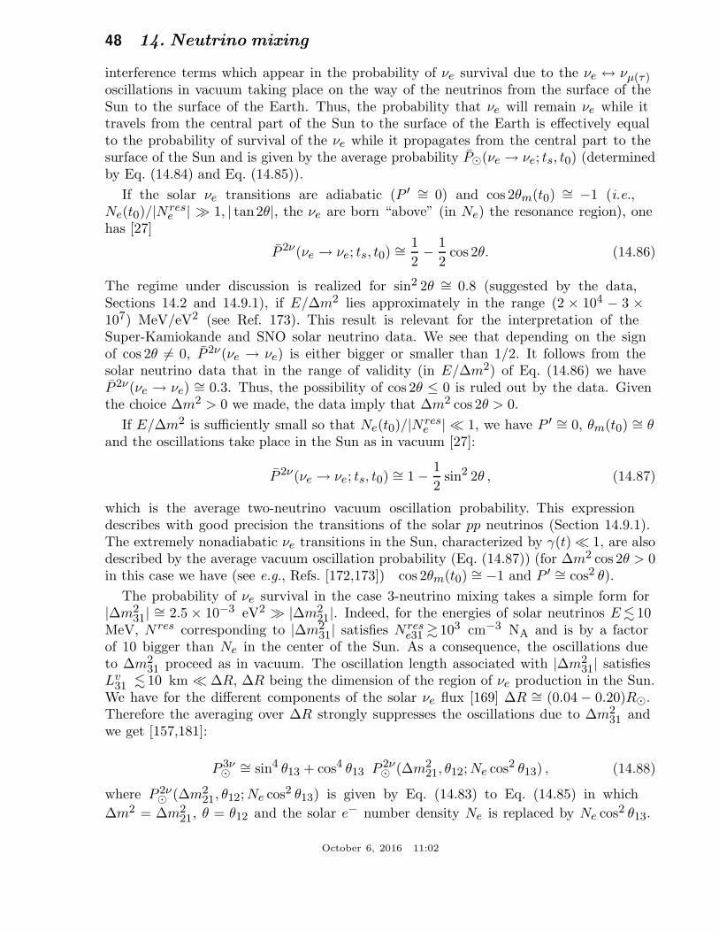
48 14. Neutrino mixing
interference terms which appear in the probability of νe survival due to the νe ↔ νµ(τ)oscillations in vacuum taking place on the way of the neutrinos from the surface of theSun to the surface of the Earth. Thus, the probability that νe will remain νe while ittravels from the central part of the Sun to the surface of the Earth is effectively equalto the probability of survival of the νe while it propagates from the central part to thesurface of the Sun and is given by the average probability P⊙(νe → νe; ts, t0) (determinedby Eq. (14.84) and Eq. (14.85)).
If the solar νe transitions are adiabatic (P ′ ∼= 0) and cos 2θm(t0) ∼= −1 (i.e.,Ne(t0)/|Nres
e | ≫ 1, | tan2θ|, the νe are born “above” (in Ne) the resonance region), onehas [27]
P 2ν(νe → νe; ts, t0) ∼=1
2− 1
2cos 2θ. (14.86)
The regime under discussion is realized for sin2 2θ ∼= 0.8 (suggested by the data,Sections 14.2 and 14.9.1), if E/∆m2 lies approximately in the range (2 × 10⁴ − 3 ×10⁷) MeV/eV2 (see Ref. 173). This result is relevant for the interpretation of theSuper-Kamiokande and SNO solar neutrino data. We see that depending on the signof cos 2θ 6= 0, P 2ν(νe → νe) is either bigger or smaller than 1/2. It follows from thesolar neutrino data that in the range of validity (in E/∆m2) of Eq. (14.86) we haveP 2ν(νe → νe) ∼= 0.3. Thus, the possibility of cos 2θ ≤ 0 is ruled out by the data. Giventhe choice ∆m2 > 0 we made, the data imply that ∆m2 cos 2θ > 0.
If E/∆m2 is sufficiently small so that Ne(t0)/|Nrese | ≪ 1, we have P ′ ∼= 0, θm(t0) ∼= θ
and the oscillations take place in the Sun as in vacuum [27]:
P 2ν(νe → νe; ts, t0) ∼= 1 − 1
2sin2 2θ , (14.87)
which is the average two-neutrino vacuum oscillation probability. This expressiondescribes with good precision the transitions of the solar pp neutrinos (Section 14.9.1).The extremely nonadiabatic νe transitions in the Sun, characterized by γ(t) ≪ 1, are alsodescribed by the average vacuum oscillation probability (Eq. (14.87)) (for ∆m2 cos 2θ > 0in this case we have (see e.g., Refs. [172,173]) cos 2θm(t0) ∼= −1 and P ′ ∼= cos2 θ).
The probability of νe survival in the case 3-neutrino mixing takes a simple form for|∆m2
31| ∼= 2.5 × 10⁻³ eV2 ≫ |∆m221|. Indeed, for the energies of solar neutrinos E . 10
MeV, Nres corresponding to |∆m231| satisfies Nres
e31 & 103 cm−3 NA and is by a factorof 10 bigger than Ne in the center of the Sun. As a consequence, the oscillations dueto ∆m2
31 proceed as in vacuum. The oscillation length associated with |∆m231| satisfies
Lv31 . 10 km ≪ ∆R, ∆R being the dimension of the region of νe production in the Sun.
We have for the different components of the solar νe flux [169] ∆R ∼= (0.04 − 0.20)R⊙.Therefore the averaging over ∆R strongly suppresses the oscillations due to ∆m2
31 andwe get [157,181]:
P 3ν⊙
∼= sin4 θ13 + cos4 θ13 P 2ν⊙ (∆m2
21, θ12; Ne cos2 θ13) , (14.88)
where P 2ν⊙ (∆m2
21, θ12; Ne cos2 θ13) is given by Eq. (14.83) to Eq. (14.85) in which
∆m2 = ∆m221, θ = θ12 and the solar e− number density Ne is replaced by Ne cos2 θ13.
October 6, 2016 11:02
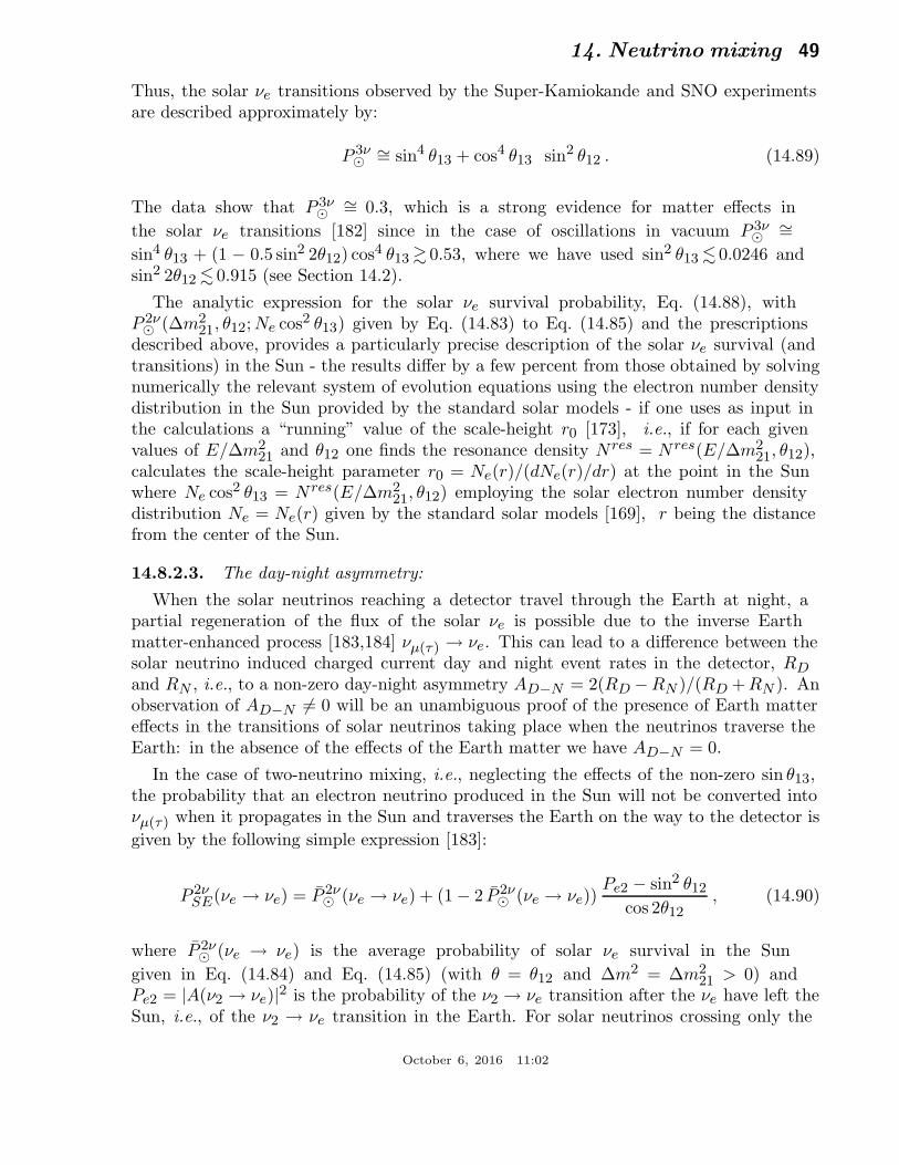
14. Neutrino mixing 49
Thus, the solar νe transitions observed by the Super-Kamiokande and SNO experimentsare described approximately by:
P 3ν⊙
∼= sin4 θ13 + cos4 θ13 sin2 θ12 . (14.89)
The data show that P 3ν⊙
∼= 0.3, which is a strong evidence for matter effects in
the solar νe transitions [182] since in the case of oscillations in vacuum P 3ν⊙
∼=sin4 θ13 + (1 − 0.5 sin2 2θ12) cos4 θ13 & 0.53, where we have used sin2 θ13 . 0.0246 andsin2 2θ12 . 0.915 (see Section 14.2).
The analytic expression for the solar νe survival probability, Eq. (14.88), withP 2ν⊙ (∆m2
21, θ12; Ne cos2 θ13) given by Eq. (14.83) to Eq. (14.85) and the prescriptionsdescribed above, provides a particularly precise description of the solar νe survival (andtransitions) in the Sun - the results differ by a few percent from those obtained by solvingnumerically the relevant system of evolution equations using the electron number densitydistribution in the Sun provided by the standard solar models - if one uses as input inthe calculations a “running” value of the scale-height r0 [173], i.e., if for each givenvalues of E/∆m2
21 and θ12 one finds the resonance density Nres = Nres(E/∆m221, θ12),
calculates the scale-height parameter r0 = Ne(r)/(dNe(r)/dr) at the point in the Sunwhere Ne cos2 θ13 = Nres(E/∆m2
21, θ12) employing the solar electron number densitydistribution Ne = Ne(r) given by the standard solar models [169], r being the distancefrom the center of the Sun.
14.8.2.3. The day-night asymmetry:
When the solar neutrinos reaching a detector travel through the Earth at night, apartial regeneration of the flux of the solar νe is possible due to the inverse Earthmatter-enhanced process [183,184] νµ(τ) → νe. This can lead to a difference between thesolar neutrino induced charged current day and night event rates in the detector, RDand RN , i.e., to a non-zero day-night asymmetry AD−N = 2(RD −RN )/(RD + RN ). Anobservation of AD−N 6= 0 will be an unambiguous proof of the presence of Earth mattereffects in the transitions of solar neutrinos taking place when the neutrinos traverse theEarth: in the absence of the effects of the Earth matter we have AD−N = 0.
In the case of two-neutrino mixing, i.e., neglecting the effects of the non-zero sin θ13,the probability that an electron neutrino produced in the Sun will not be converted intoνµ(τ) when it propagates in the Sun and traverses the Earth on the way to the detector is
given by the following simple expression [183]:
P 2νSE(νe → νe) = P 2ν
⊙ (νe → νe) + (1 − 2 P 2ν⊙ (νe → νe))
Pe2 − sin2 θ12
cos 2θ12, (14.90)
where P 2ν⊙ (νe → νe) is the average probability of solar νe survival in the Sun
given in Eq. (14.84) and Eq. (14.85) (with θ = θ12 and ∆m2 = ∆m221 > 0) and
Pe2 = |A(ν2 → νe)|2 is the probability of the ν2 → νe transition after the νe have left theSun, i.e., of the ν2 → νe transition in the Earth. For solar neutrinos crossing only the
October 6, 2016 11:02
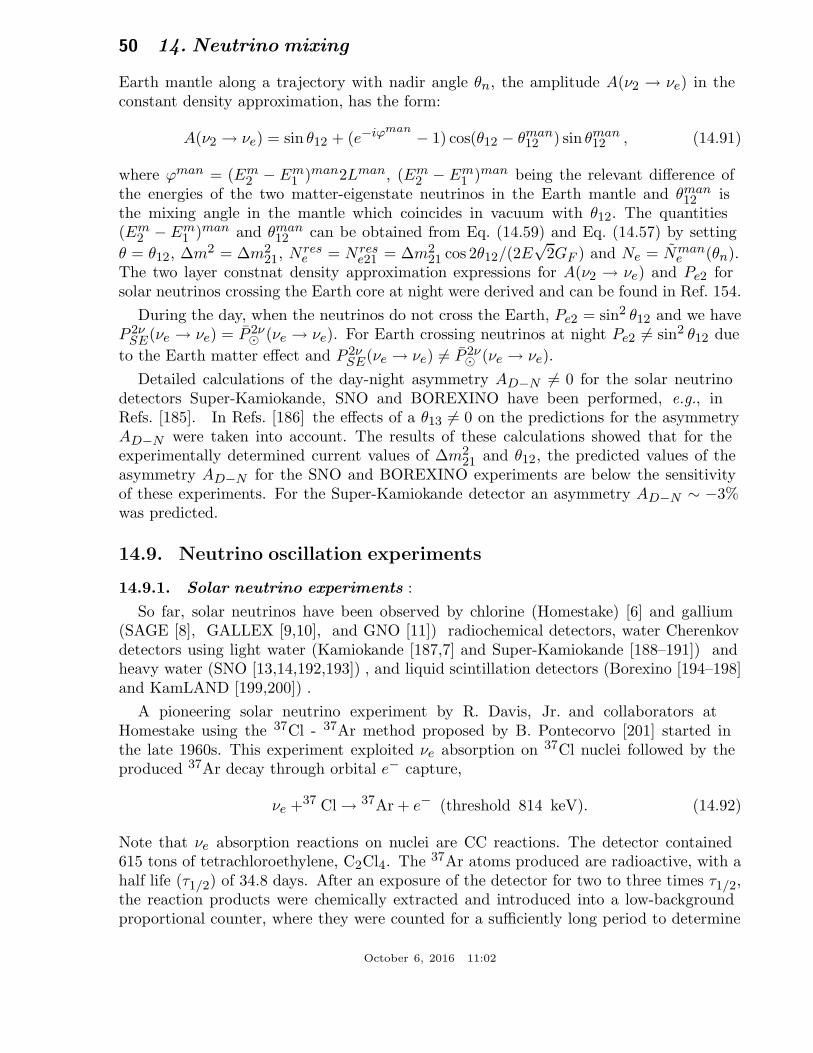
50 14. Neutrino mixing
Earth mantle along a trajectory with nadir angle θn, the amplitude A(ν2 → νe) in theconstant density approximation, has the form:
A(ν2 → νe) = sin θ12 + (e−iϕman − 1) cos(θ12 − θman12 ) sin θman
12 , (14.91)
where ϕman = (Em2 − Em
1 )man2Lman, (Em2 − Em
1 )man being the relevant difference ofthe energies of the two matter-eigenstate neutrinos in the Earth mantle and θman
12 isthe mixing angle in the mantle which coincides in vacuum with θ12. The quantities(Em
2 − Em1 )man and θman
12 can be obtained from Eq. (14.59) and Eq. (14.57) by setting
θ = θ12, ∆m2 = ∆m221, Nres
e = Nrese21 = ∆m2
21 cos 2θ12/(2E√
2GF ) and Ne = Nmane (θn).
The two layer constnat density approximation expressions for A(ν2 → νe) and Pe2 forsolar neutrinos crossing the Earth core at night were derived and can be found in Ref. 154.
During the day, when the neutrinos do not cross the Earth, Pe2 = sin2 θ12 and we haveP 2ν
SE(νe → νe) = P 2ν⊙ (νe → νe). For Earth crossing neutrinos at night Pe2 6= sin2 θ12 due
to the Earth matter effect and P 2νSE(νe → νe) 6= P 2ν
⊙ (νe → νe).
Detailed calculations of the day-night asymmetry AD−N 6= 0 for the solar neutrinodetectors Super-Kamiokande, SNO and BOREXINO have been performed, e.g., inRefs. [185]. In Refs. [186] the effects of a θ13 6= 0 on the predictions for the asymmetryAD−N were taken into account. The results of these calculations showed that for theexperimentally determined current values of ∆m2
21 and θ12, the predicted values of theasymmetry AD−N for the SNO and BOREXINO experiments are below the sensitivityof these experiments. For the Super-Kamiokande detector an asymmetry AD−N ∼ −3%was predicted.
14.9. Neutrino oscillation experiments
14.9.1. Solar neutrino experiments :
So far, solar neutrinos have been observed by chlorine (Homestake) [6] and gallium(SAGE [8], GALLEX [9,10], and GNO [11]) radiochemical detectors, water Cherenkovdetectors using light water (Kamiokande [187,7] and Super-Kamiokande [188–191]) andheavy water (SNO [13,14,192,193]) , and liquid scintillation detectors (Borexino [194–198]and KamLAND [199,200]) .
A pioneering solar neutrino experiment by R. Davis, Jr. and collaborators atHomestake using the 37Cl - 37Ar method proposed by B. Pontecorvo [201] started inthe late 1960s. This experiment exploited νe absorption on 37Cl nuclei followed by theproduced 37Ar decay through orbital e− capture,
νe +37 Cl → 37Ar + e− (threshold 814 keV). (14.92)
Note that νe absorption reactions on nuclei are CC reactions. The detector contained615 tons of tetrachloroethylene, C2Cl4. The 37Ar atoms produced are radioactive, with ahalf life (τ1/2) of 34.8 days. After an exposure of the detector for two to three times τ1/2,the reaction products were chemically extracted and introduced into a low-backgroundproportional counter, where they were counted for a sufficiently long period to determine
October 6, 2016 11:02
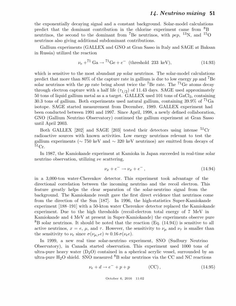
14. Neutrino mixing 51
the exponentially decaying signal and a constant background. Solar-model calculationspredict that the dominant contribution in the chlorine experiment came from 8Bneutrinos, the second to the dominant from 7Be neutrinos, with pep, 13N, and 15Oneutrinos also giving additional subdominant contributions.
Gallium experiments (GALLEX and GNO at Gran Sasso in Italy and SAGE at Baksanin Russia) utilized the reaction
νe +71 Ga → 71Ge + e− (threshold 233 keV), (14.93)
which is sensitive to the most abundant pp solar neutrinos. The solar-model calculationspredict that more than 80% of the capture rate in gallium is due to low energy pp and 7Besolar neutrinos with the pp rate being about twice the 7Be rate. The 71Ge atoms decaythrough electron capture with a half life (τ1/2) of 11.43 days. SAGE used approximately50 tons of liquid gallium metal as a a target. GALLEX used 101 tons of GaCl3, containing30.3 tons of gallium. Both experiments used natural gallium, containing 39.9% of 71Gaisotope. SAGE started measurement from December, 1989. GALLEX experiment hadbeen conducted between 1991 and 1997. Since April, 1998, a newly defined collaboration,GNO (Gallium Neutrino Observatory) continued the gallium experiment at Gran Sassountil April 2003.
Both GALLEX [202] and SAGE [203] tested their detectors using intense 51Crradioactive sources with known activities. Low energy neutrinos relevant to test thegallium experiments (∼ 750 keV and ∼ 320 keV neutrinos) are emitted from decays of51Cr.
In 1987, the Kamiokande experiment at Kamioka in Japan succeeded in real-time solarneutrino observation, utilizing νe scattering,
νx + e− → νx + e− , (14.94)
in a 3,000-ton water-Cherenkov detector. This experiment took advantage of thedirectional correlation between the incoming neutrino and the recoil electron. Thisfeature greatly helps the clear separation of the solar-neutrino signal from thebackground. The Kamiokande result gave the first direct evidence that neutrinos comefrom the direction of the Sun [187]. In 1996, the high-statistics Super-Kamiokandeexperiment [188–191] with a 50-kton water Cherenkov detector replaced the Kamiokandeexperiment. Due to the high thresholds (recoil-electron total energy of 7 MeV inKamiokande and 4 MeV at present in Super-Kamiokande) the experiments observe pure8B solar neutrinos. It should be noted that the reaction (Eq. (14.94)) is sensitive to allactive neutrinos, x = e, µ, and τ . However, the sensitivity to νµ and ντ is smaller thanthe sensitivity to νe since σ(νµ,τe) ≈ 0.16 σ(νee).
In 1999, a new real time solar-neutrino experiment, SNO (Sudbury NeutrinoObservatory), in Canada started observation. This experiment used 1000 tons ofultra-pure heavy water (D2O) contained in a spherical acrylic vessel, surrounded by anultra-pure H2O shield. SNO measured 8B solar neutrinos via the CC and NC reactions
νe + d → e− + p + p (CC) , (14.95)
October 6, 2016 11:02
52 14. Neutrino mixing
andνx + d → νx + p + n (NC) , (14.96)
as well as νe scattering, (Eq. (14.94)). The CC reaction, (Eq. (14.95)), is sensitive only toνe, while the NC reaction, (Eq. (14.96)), is sensitive to all active neutrinos. This is a keyfeature to solve the solar neutrino problem. If it is caused by flavour transitions such asneutrino oscillations, the solar neutrino fluxes measured by CC and NC reactions wouldshow a significant difference.
The Q-value of the CC reaction is −1.4 MeV and the e− energy is strongly correlatedwith the νe energy. Thus, the CC reaction provides an accurate measure of the shapeof the 8B neutrino spectrum. The contributions from the CC reaction and νe scatteringcan be distinguished by using different cos θ distributions, where θ is the angle of thee− momentum with respect to the Sun-Earth axis. While the νe scattering events havea strong forward peak, CC events have an approximate angular distribution of (1 − 1/3cosθ).
The neutrino energy threshold of the NC reaction is 2.2 MeV. In the pure D2O [13,14],the signal of the NC reaction was neutron capture in deuterium, producing a 6.25-MeVγ-ray. In this case, the capture efficiency was low and the deposited energy was close tothe detection threshold of 5 MeV. In order to enhance both the capture efficiency andthe total γ-ray energy (8.6 MeV), 2 tons of NaCl was added to the heavy water in thesecond phase of the experiment [192]. Subsequently NaCl was removed and an arrayof 3He neutron counters were installed for the third phase measurement [193]. Theseneutron counters provided independent NC measurement with different systematics fromthat of the second phase, and thus strengthened the reliability of the NC measurement.The SNO experiment completed data acquisition in 2006.
Another real time solar neutrino experiment, Borexino at Gran Sasso, started solarneutrino observation in 2007. This experiment measures solar neutrinos via νe scatteringin 300 tons of ultra-pure liquid scintillator. With a detection threshold as low as 250 keV,the flux of monochromatic 0.862 MeV 7Be solar neutrinos has been directly observedfor the first time [194]. Further, Borexino measured the fluxes of monochromatic 1.44MeV pep solar neutrinos [195] and pp solar neutrinos [196], both for the first time.Measurements of these low energy solar neutrinos are important not only to test the SSMfurther, but also to study the MSW effect over the energy region spanning from sub-MeVto 10 MeV.
KamLAND is a 1-kton ultra-pure liquid scintillator detector located at the oldKamiokande’s site. Recently this experiment also measured the 7Be solar neutrinoflux [199]. As KamLAND is a multi-purpose experiment with one of the primary goalsto be a long-baseline neutrino oscillation studies using electron antineutrinos emittedfrom nuclear power reactors, further description of the KamLAND experiment is givenlater in Section 14.9.4.
October 6, 2016 11:02
14. Neutrino mixing 53
14.9.2. Atmospheric neutrino oscillation experiments :
Almost all large underground detectors can observe atmospheric neutrinos. In theearly history of neutrino oscillation studies using atmospheric neutrinos, water Cherenkovdetectors for Kamiokande [204,205] and IMB [206] (experiment in the US) and irontracking calorimeters for the Frejus experiment [207] in France and the Soudan 2experiment [208] at the Soudan mine in the US, measured atmospheric neutrinos, inparticular, the Φ(νµ + νµ)/Φ(νe + νe) ratio. The main purpose of all these experimentswas search for nucleon decay, and atmospheric neutrinos were backgrounds for themain purpose. Following these initial experiments, Super-Kamiokande discovered theatmospheric neutrino oscillation [17], and a multi-purpose detector MACRO [209] atGran Sasso obtained results consistent with neutrino oscillation. Later, the far detectorof the MINOS long baseline neutrino oscillation experiment also measured atmosphericneutrinos [210], and obtained results consistent with atmospheric neutrino oscillation.This detector is a 5.4 kton iron-scintillator tracking calorimeter with toroidal magneticfield.
Atmospheric neutrino oscillations have also been observed by the neutrino telescopesfor high-energy neutrino astronomy (TeV ∼ PeV) using Cherenkov technique, ANTARESand IceCube-DeepCore, based on the measurement of νµ charged-current events havingan upward-going muon track to avoid contamination from atmospheric muon background.ANTARES [211] is an open water detector deployed deep under the Mediterranean Sea(depth ∼ 2500 m) 40 km off-shore from Toulon, France, while IceCube [212] is a detectordeployed in the ice at the South Pole at the depth from 1450 m to 2450 m. Thoughboth experiments are optimized to high-energy neutrino interactions in the TeV range,they need to measure muon neutrinos with energies as low as ∼ 20 GeV in order to besensitive to atmospheric neutrino oscillations. ANTARES could reconstruct upward-goingmuons from νµ interactions down to 20 GeV [213], while IceCube used the low-energysub-detector DeepCore, a region of denser IceCube instrumentation, to lower the muonneutrino energy threshold down to 10 GeV [214] (also see Ref. 215 with 20 GeVthreshold).
All these detectors, with the exception of the MINOS far detector, cannot measurethe charge of the final-state leptons, and, therefore, neutrino and antineutrino inducedevents cannot be discriminated; the MINOS far detector can measure the charge ofthe muon track, and, therefore, identify νµ and νµ charged-current events. However,all these detectors can identify the final-state leptons to be µ-like or e-like. TakingSuper-Kamiokande as an example, neutrino events having their vertex in the 22.5 ktonfiducial volume are classified into fully contained (FC) events and partially contained (PC)events. The FC events are required to have no activity in the anti-counter. Single-ringevents have only one charged lepton which radiates Cherenkov light in the final state,and particle identification is particularly clean for single-ring FC events. A ring producedby an e-like (e±, γ) particle exhibits a more diffuse pattern than that produced by aµ-like (µ±, π±) particle, since an e-like particle produces an electromagnetic shower andlow-energy electrons suffer considerable multiple Coulomb scattering in water. All the PCevents are assumed to be µ-like since the PC events comprise a 98% pure charged-currentνµ sample.
October 6, 2016 11:02
54 14. Neutrino mixing
In the near future, Super-Kamiokande and the MINOS (now MINOS+ [216]) fardetector will continue atmospheric neutrino measurements. In addition, currently severallarge underground detectors are proposed for construction (liquid argon detectors with atotal mass of 10 - 40 kton as the far detector of the DUNE experiment [84] in the US,and a 1 Mton water Cherenkov detector, Hyper-Kamiokande [165], as the far detector ofthe T2HK experiment [85] in Japan) or approved (a 50 kton magnetized iron trackingcalorimeter, ICAL at the INO (India-based Neutrino Observatory) [219] in the southernIndian state of Tamil Nadu).
As high-statistics atmospheric neutrino observations in the energy region of a fewto ∼ 10 GeV are considered to be promising for the determination of the neutrinomass ordering, see Section 14.8, there are two proposed densely-instrumented neutrinotelescopes PINGU (Precision IceCube Next-Generation Upgrade) [220] and ORCA(Oscillation Research with Cosmics in the Abyss) [221], both having a multi-megatontotal mass. PINGU will be deployed inside the DeepCore, and will be sensitive to > 1GeV. ORCA is proposed as part of the second phase of the KM3NeT [222], a network ofneutrino telescopes deep under the Mediterranean Sea. ORCA will have sensitivity downto a few GeV, its site being Toulon, France.
14.9.3. Accelerator neutrino oscillation experiments :
For earlier accelerator neutrino oscillation experiments before the discovery of theatmospheric neutrino oscillation, see, e.g., Ref. 223. The ∆m2 ≥ 2 × 10⁻³ eV2 regioncan be explored by accelerator-based long-baseline experiments with typically E ∼ 1GeV and L ∼ several hundred km. With a fixed baseline distance and a narrower,well understood neutrino energy spectrum, the value of |∆m2
31(32)| and, with higher
statistics, also the relevant neutrino mixing angle, are potentially better constrained inaccelerator experiments than from atmospheric neutrino observations. With νµ → νe
appearance measurements, accelerator long-baseline experiments can measure θ13 withinan uncertainty related, in particular, to the CP-violating phase δ. Using preciseresults on θ13 from reactor experiments, they can potentially determine or constrainδ and the neutrino mass ordering, depending on the experimental conditions such asbaseline distance. K2K [19], MINOS [20,21] and MINOS+ [216], OPERA [141,142],ICARUS [224], T2K [23,22], and NOνA [55,56] are completed or currently runningexperiments, and DUNE [84] and T2HK [85] are proposed future experiments.
The K2K (KEK-to-Kamioka) long-baseline neutrino oscillation experiment [19] isthe first accelerator-based experiment with a neutrino path length extending hundredsof kilometers. A horn-focused wide-band muon neutrino beam having an averageL/Eν ∼ 200 (L = 250 km, 〈Eν〉 ∼ 1.3 GeV), was produced by 12-GeV protons from theKEK-PS and directed to the Super-Kamiokande detector. A near detector was located300 m downstream of the production target. K2K experiment started data-taking in 1999and was completed in 2004.
MINOS [20,21] is the second long-baseline neutrino oscillation experiment with nearand far detectors. Neutrinos are produced by the NuMI (Neutrinos at the Main Injector)facility using 120 GeV protons from the Fermilab Main Injector. The far detector is a5.4 kton (total mass) iron-scintillator tracking calorimeter with toroidal magnetic field,
October 6, 2016 11:02
14. Neutrino mixing 55
located underground in the Soudan mine. The baseline distance is 735 km. The neardetector, located 1.04 km downstream of the production target, is also an iron-scintillatortracking calorimeter with toroidal magnetic field, with a total mass of 0.98 kton. TheNuMI neutrino beam is a horn-focused wide-band beam. Its energy spectrum can bevaried by moving the target position relative to the first horn and changing the horncurrent. MINOS started the neutrino-beam run in 2005 and was completed in 2012.Almost all the MINOS data were taken with the low-energy beam spectrum which peakedat 3 GeV. Part of the MINOS data were taken with the νµ-enhanced beam by invertingthe current in magnetic horns. In September, 2013, the MINOS+ experiment [216]started with the same near and far detectors as the MINOS experiment, but withthe medium-energy beam spectrum which peaks at 7 GeV. At zero degree, the NuMImedium-energy beam has much higher intensity than the NuMI low-energy beam.
The T2K experiment [22,23] is the first off-axis long-baseline neutrino oscillationexperiment. The baseline distance is 295 km between the J-PARC in Tokai, Japan andSuper-Kamiokande. A narrow-band νµ beam with a peak energy of 0.6 GeV, produced by30 GeV protons from the J-PARC Main Ring, is directed 2.5◦ off-axis to SK. With thisconfiguration, the νµ beam is tuned to the first oscillation minimum of the νµ survivalprobability. T2K started the first physics run in 2010.
The NOνA experiment [55,56] is an off-axis long-baseline neutrino oscillationexperiment using the the NuMI medium-energy beam. Its detectors are positioned14 mrad off-axis. With this configuration, the neutrino beam has a narrow spectrumwhich peaks at 2 GeV. The 14 kton far detector is located on the surface at AshRiver, Minnesota, 810 km from the production target. The 0.3 kton near detector islocated underground at Fermilab, approximately 1km from the target. Both detectorsare fine-grained tracking calorimeters consisting of arrays of PVC cells filled with liquidscintillator. NOνA started full operation in October, 2014.
Although the atmospheric neutrino oscillations and accelerator long-baseline νµ
disappearance data are fully consistent with the dominance of νµ → ντ oscillations for νµ
at GeV energies, ντ appearance in the muon neutrino beam has to be demonstrated. Asthe τ production threshold is Eν ∼ 3.5 GeV, a high-energy neutrino beam is needed forthis purpose. The only experiment of this kind is OPERA [141,142] with a muon neutrinosource at CERN and a detector at Gran Sasso with the baseline distance of 730 km.OPERA does not have a near detector. The CNGS (CERN Neutrinos to Gran Sasso)neutrino beam with 〈Eν〉 = 17 GeV is produced by high-energy protons from the CERNSPS. OPERA received the CNGS neutrino beam between 2008 and 2012. The detector isa combination of the “Emulsion Cloud Chamber” and magnetized spectrometer, having atarget mass of 1,290 tons. At Gran Sasso, another neutrino experiment, ICARUS [224],with a 600-ton liquid argon detector, was located and received the CNGS neutrino beamfrom 2010 to 2012. The ICARUS detector will be transported to Fermilab by 2017, andwill be used in a short baseline experiment.
DUNE (Deep Underground Neutrino Experiment) [84] is a projected future experimentwith a 1,300 km baseline. A 10 ∼ 34 kton liquid-argon far detector will be located deepunderground at the Sanford Lab in South Dakota, the U.S. A fine-grained near neutrinodetector will be installed at Fermilab. Based on the existing NuMI beamline and a MW
October 6, 2016 11:02
56 14. Neutrino mixing
class proton source, a wide-band, high-intensity νµ beam with a peak flux at 2.5 GeVis considered for this experiment. T2HK [85] is another future long baseline experimentfrom J-PARC to the 1 Mton water Cherenkov detector, Hyper-Kamiokande [165], whichis at the proposal stage, at Kamioka. An upgrade of the J-PARC Main Ring to achieve aMW-class beam power is also proposed.
In the context of possible hints for the existence of sterile neutrinos at the eV scale,short-baseline accelerator neutrino oscillation experiments have been drawing attention.LSND [225], Karmen 2 (and Karmen 1) [226], and MiniBooNE [227,228] are completedexperiments. New short-baseline experiments, MicroBooNE, SBND, and ICARUS arein preparation at Fermilab [229]. The detectors of all these new experiments useliquid-argon TPC technology.
The LSND (Liquid Scintillation Neutrino Detector) experiment [225] used the LANSE(Los Alamos Neutron Science Center, formerly known as the LAMPF) 800 MeV protonlinac as a neutrino source. At this energy, kaon production is negligible. Most of theproduced positive pions stop in the massive target and decay at rest, with decay muonsalso stop in the target and decay. Most of the produced negative pions also stop in thetarget and are absorbed by the target nuclei. Therefore, this neutrino source emits νµ,νµ, and νe, with very small contamination of νe which comes from π− decay in flightfollowed by the µ− decay at rest. Because of this small νe component in the neutrino flux,LSND made a sensitive search for νµ → νe appearance with 167 tons of diluted liquidscintillator in a tank located about 30 m from the neutrino source, using the reactionνe + p → e+ + n. Also, LSND studied νµ → νe appearance above the Michel electronendpoint energy using the reaction νe + C → e− + N , as the νe flux from µ+ decay inflight is suppressed due to the long muon lifetime and that from π+ decay in flight issuppressed by the small π+ → e+ + νe branching ratio. The Karmen 2 experiment [226]used the 800 MeV proton synchrotron at the neutron spallation facility of the RutherfordAppleton Laboratory, also to produce low-energy νµ flux from µ+ decay at rest. TheKarmen 2 detector is a segmented liquid scintillator calorimeter located at a distance of17.7 m from the neutrino source. MiniBooNE used a conventional horn-focused neutrinobeam produced by 8 GeV protons from the Fermilab booster synchrotron. MiniBooNEinvestigated both νe [227] and νe [228] appearance in νµ and νµ beams, respectively,with a detector containing 806 tons of mineral oil and located 541 m downstream of theproduction target.
14.9.4. Reactor neutrino oscillation experiments :
As the relevant energy range of the events detected in the reactor experiment is < 10MeV, detection of a prompt positron signal and delayed neutron signal in coincidence isimportant to identify the inverse β-decay, rejecting natural backgrounds. For detectingneutrons effectively, gadolinium-loaded liquid scintillator is widely used. While neutroncapture on a hydrogen produces a 2.2 MeV γ, neutron capture on Gd produces multipleγ, each having average energy of ∼ 2 MeV, giving a ∼ 8 MeV signal in total.
For short baseline reactor νe neutrino oscillation experiments in 1980s or earlier, see,e.g., Refs. [230,46]. Reactor νe disappearance experiments with L ∼ 1 km, 〈E〉 ∼ 3MeV are sensitive to E/L ∼ 3 × 10⁻³ eV2 ∼ |∆m2
31(32)|. At this baseline distance, the
October 6, 2016 11:02
14. Neutrino mixing 57
reactor νe oscillations driven by ∆m221 are negligible. Therefore, as can be seen from
Eq. (14.44) and Eq. (14.46), θ13 can be directly measured. An experiment at the ChoozNuclear Power Station in France [51] was the first experiment of this kind. The detectorwas located in an underground laboratory with 300 mwe (meter water equivalent) rockoverburden, at about 1 km from the neutrino source. It consisted of a central 5-ton targetfilled with 0.09% Gd-loaded liquid scintillator, surrounded by an intermediate 17-ton andouter 90-ton regions filled with Gd-free liquid scintillator. Another experiment at thePalo Verde Nuclear Generating Station in Arizona, United States, also searched for νe
disappearance using 11.34 tons of Gd-loaded liquid scintillator located at a shallow (32mwe) underground site, about 800 m from the neutrino source [231].
Although these two experiments in the late 1990s had found no evidence for νe
disappearance, after establishment of atmospheric and solar neutrino oscillations theimportance of the reactor neutrino oscillation experiment to measure θ13 was widelyrecognized, and this led to the realization of the three new reactor experiments,Double Chooz in France, RENO in Korea, and Daya Bay in China. The Double Choozexperiment [30,33] measures electron antineutrinos from two 4.25 GWth reactors with afar detector at an average distance of 1050 m from the two reactor cores. The Daya Bayexperiment [31,35] measures νes from the Daya Bay nuclear power complex (six 2.9 GWthreactors), initially with six functionally identical detectors deployed in two near (470 mand 576 m of flux-weighted baselines) and one far (1648 m) underground halls. The firstDaya Bay result [31] was obtained with this detector configuration. Later, two detectorswere further installed, one in one of the near detector hall and the other in the fardetetor hall. The RENO experiment [32] measures electron antineutrinos from four 2.8GWth and two 2.66 GWth reactors at Yonggwang Nuclear Power Plant with two identicaldetectors located at 294 m and 1383 m from the reactor array center (or flux-weightedbaseline distance of 408.56 m and 1443.99 m, respectively). Antineutrino detectors ofthese experiments have similar structures. They consist of three layers and an opticallyindependent outer veto detector. The innermost layer of the antineutrino detector is filledwith Gd-loaded liquid scintillator, which is surrounded by a “γ-catcher” layer filled withGd-free liquid scintillator, and outside the γ-catcher is a buffer layer filled with mineraloil. An outer veto detector is filled with purified water (Daya Bay and RENO) or liquidscintillator (Double Chooz). In addition, the Double Chooz near detector tank is shieldedby a 1 m thick water buffer. RENO and Daya Bay started measurements with both thenear and far detectors from the beginning. However, the Double Chooz near detector hasbeen completed at the end of 2014. All these experiments published their first results onreactor νe disappearance in 2012.
For longer baseline distance of L ∼ a few hundred km, a reactor neutrino oscillationexperiment is sensitive to ∆m2 down to ∼ 10−5 eV2. Therefore, such an experiment cantest the LMA (Large Mixing Angle) solution of the solar neutrino problem, assumingCPT invariance. However, a higher νe flux and a larger target mass are needed comparedto short-baseline reactor experiments to obtain statistically significant event rate. So far,KamLAND is the only experiment of this kind. It is located at the old Kamiokande’ssite in Japan. Its neutrino target is 1-kton ultra-pure liquid scintillator contained in atransparent balloon, which is hold inside a spherical tank with buffer oil filled between
October 6, 2016 11:02
58 14. Neutrino mixing
the baloon and the tank. The tank is surrounded by an outer water Cherenkov detector.Before the Great East Japan Earthquake in March 2011, many nuclear reactors wereoperating in Japan, and more than 79% of the νe flux at KamLAND was coming from 26reactors between 138 - 214 km away, with a flux-weighted average distance of ∼ 180 km.
In future, medium baseline (∼ 50 km) reactor neutrino oscillation experimentswith neutrino target mass of ∼ 20 kton and with a very good energy resolution of3%/
√
Eν(MeV), not reached in any previous experiment with liquid scintillator, areaiming, in particular, to determine the type of spectrum the neutrino masses obey, i.e.,the neutrino mass ordering (see Section 14.2). These experiments have additional richphysics program. The Jiangmen Underground Neutrino Observatory (JUNO) [232] atKaiping, Jiangmen in Southern China will be located at 53 km from both of the plannedYangjiang and Taishan nuclear power plants. The neutrino target of this experiment willbe 20 kton liquid scintillator. JUNO is a funded project, and its construction started inJanuary, 2015. A similar experiment, RENO50 [127], is also proposed in Korea.
14.10. Results of solar neutrino experiments and KamLAND
In 1967, analyzing the possible effects of neutrino oscillations on the solar neutrinoflux measurements, B. Pontecorvo predicted the solar neutrino “deficit” in experimentsdetecting solar neutrinos via a CC reaction [1] before the first solar neutrino data wereavailable. The solar-neutrino problem, i.e., the problem of understanding the origin ofthe observed deficit of solar neutrinos, remained unsolved for more than 30 years sincethe late 1960s, but solar neutrino experiments have achieved remarkable progress sincethe beginning of the new century, and the solar-neutrino problem has been understood asdue to neutrino flavour conversion.
14.10.1. Measurements of ∆m2
21and θ12 :
From the very beginning of the solar-neutrino observation by the Homestake chlorineexperiment [233] in the late 1960s, it was recognized that the observed flux wassignificantly smaller than the SSM prediction. The subsequent radiochemical solarneutrino experiments using 71Ga, SAGE [234] and GALLEX [9] also reported smallersolar neutrino fluxes than the SSM predictions in the early 1990s. final results of theseexperiments [235] are compared with the SSM predictions in Table 14.5. Experimentswith water Cherenkov detectors, Kamiokande and Super-Kamiokande, observed almostpure 8B solar neutrinos through νe elastic scattering, and they also reported a cleardeficit of 8B solar neutrino flux.
In 2001, the initial SNO CC result combined with the Super-Kamiokande’s high-statistics νe elastic scattering result [236] provided direct evidence for flavour conversionof solar neutrinos [13]. Later, SNO’s NC measurements further strengthened thisconclusion [14,192,193]. From the salt-phase measurement [192], the fluxes measuredwith CC, ES, and NC events were obtained as
φCCSNO = (1.68 ± 0.06+0.08
−0.09) × 106cm−2s−1 , (14.97)
φESSNO = (2.35 ± 0.22 ± 0.15) × 106cm−2s−1 , (14.98)
October 6, 2016 11:02
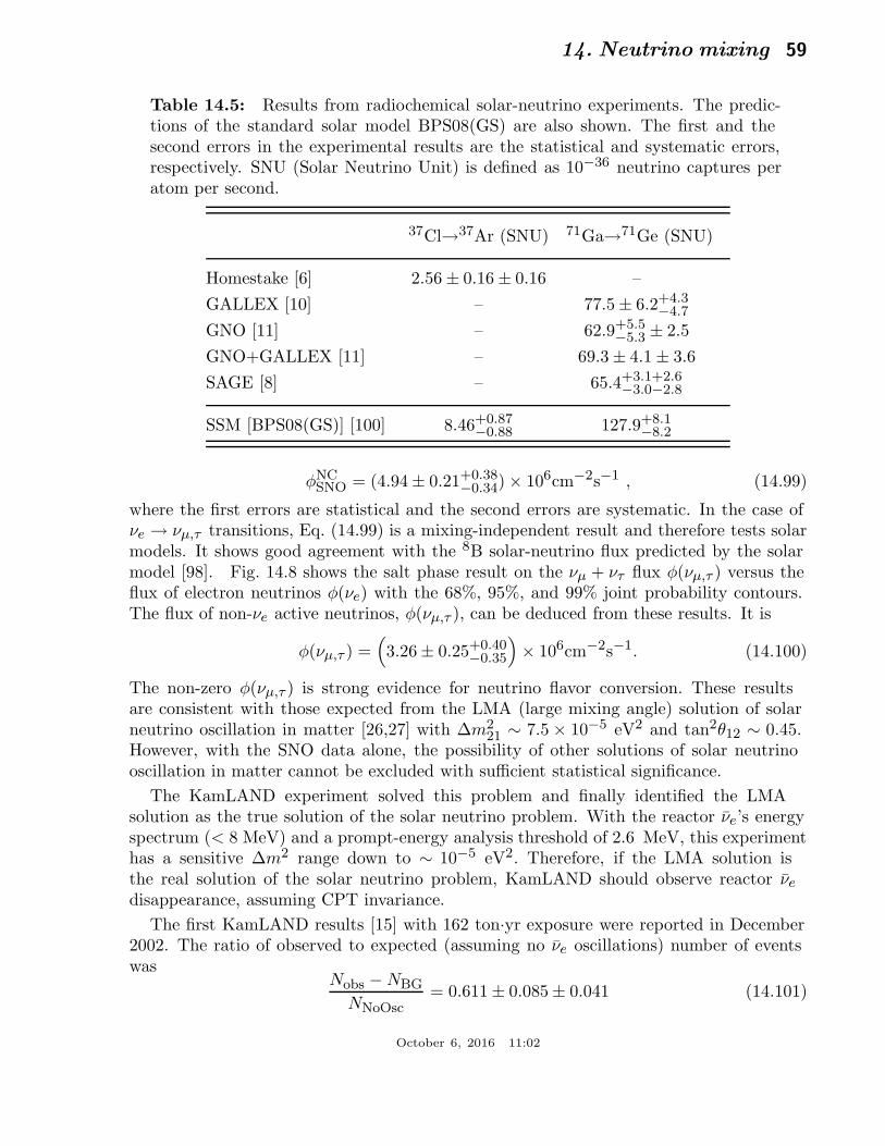
14. Neutrino mixing 59
Table 14.5: Results from radiochemical solar-neutrino experiments. The predic-tions of the standard solar model BPS08(GS) are also shown. The first and thesecond errors in the experimental results are the statistical and systematic errors,respectively. SNU (Solar Neutrino Unit) is defined as 10−36 neutrino captures peratom per second.
37Cl→37Ar (SNU) 71Ga→71Ge (SNU)
Homestake [6] 2.56 ± 0.16 ± 0.16 –
GALLEX [10] – 77.5 ± 6.2+4.3−4.7
GNO [11] – 62.9+5.5−5.3 ± 2.5
GNO+GALLEX [11] – 69.3 ± 4.1 ± 3.6
SAGE [8] – 65.4+3.1+2.6−3.0−2.8
SSM [BPS08(GS)] [100] 8.46+0.87−0.88 127.9+8.1
−8.2
φNCSNO = (4.94 ± 0.21+0.38
−0.34) × 106cm−2s−1 , (14.99)
where the first errors are statistical and the second errors are systematic. In the case ofνe → νµ,τ transitions, Eq. (14.99) is a mixing-independent result and therefore tests solarmodels. It shows good agreement with the 8B solar-neutrino flux predicted by the solarmodel [98]. Fig. 14.8 shows the salt phase result on the νµ + ντ flux φ(νµ,τ ) versus theflux of electron neutrinos φ(νe) with the 68%, 95%, and 99% joint probability contours.The flux of non-νe active neutrinos, φ(νµ,τ ), can be deduced from these results. It is
φ(νµ,τ ) =(
3.26 ± 0.25+0.40−0.35
)
× 106cm−2s−1. (14.100)
The non-zero φ(νµ,τ ) is strong evidence for neutrino flavor conversion. These resultsare consistent with those expected from the LMA (large mixing angle) solution of solarneutrino oscillation in matter [26,27] with ∆m2
21 ∼ 7.5 × 10⁻⁵ eV2 and tan2θ12 ∼ 0.45.However, with the SNO data alone, the possibility of other solutions of solar neutrinooscillation in matter cannot be excluded with sufficient statistical significance.
The KamLAND experiment solved this problem and finally identified the LMAsolution as the true solution of the solar neutrino problem. With the reactor νe’s energyspectrum (< 8 MeV) and a prompt-energy analysis threshold of 2.6 MeV, this experimenthas a sensitive ∆m2 range down to ∼ 10−5 eV2. Therefore, if the LMA solution isthe real solution of the solar neutrino problem, KamLAND should observe reactor νe
disappearance, assuming CPT invariance.
The first KamLAND results [15] with 162 ton·yr exposure were reported in December2002. The ratio of observed to expected (assuming no νe oscillations) number of eventswas
Nobs − NBG
NNoOsc= 0.611 ± 0.085 ± 0.041 (14.101)
October 6, 2016 11:02
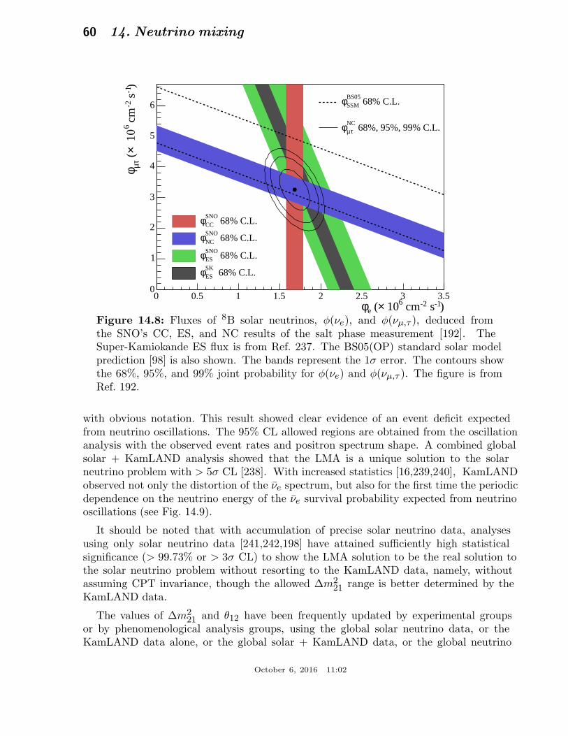
60 14. Neutrino mixing
)-1 s-2 cm6 10× (eφ0 0.5 1 1.5 2 2.5 3 3.5
)-1
s-2
cm
6
10
× ( τµφ
0
1
2
3
4
5
6
68% C.L.CCSNOφ
68% C.L.NCSNOφ
68% C.L.ESSNOφ
68% C.L.ESSKφ
68% C.L.SSMBS05φ
68%, 95%, 99% C.L.τµNCφ
Figure 14.8: Fluxes of 8B solar neutrinos, φ(νe), and φ(νµ,τ ), deduced fromthe SNO’s CC, ES, and NC results of the salt phase measurement [192]. TheSuper-Kamiokande ES flux is from Ref. 237. The BS05(OP) standard solar modelprediction [98] is also shown. The bands represent the 1σ error. The contours showthe 68%, 95%, and 99% joint probability for φ(νe) and φ(νµ,τ ). The figure is fromRef. 192.
with obvious notation. This result showed clear evidence of an event deficit expectedfrom neutrino oscillations. The 95% CL allowed regions are obtained from the oscillationanalysis with the observed event rates and positron spectrum shape. A combined globalsolar + KamLAND analysis showed that the LMA is a unique solution to the solarneutrino problem with > 5σ CL [238]. With increased statistics [16,239,240], KamLANDobserved not only the distortion of the νe spectrum, but also for the first time the periodicdependence on the neutrino energy of the νe survival probability expected from neutrinooscillations (see Fig. 14.9).
It should be noted that with accumulation of precise solar neutrino data, analysesusing only solar neutrino data [241,242,198] have attained sufficiently high statisticalsignificance (> 99.73% or > 3σ CL) to show the LMA solution to be the real solution tothe solar neutrino problem without resorting to the KamLAND data, namely, withoutassuming CPT invariance, though the allowed ∆m2
21 range is better determined by theKamLAND data.
The values of ∆m221 and θ12 have been frequently updated by experimental groups
or by phenomenological analysis groups, using the global solar neutrino data, or theKamLAND data alone, or the global solar + KamLAND data, or the global neutrino
October 6, 2016 11:02
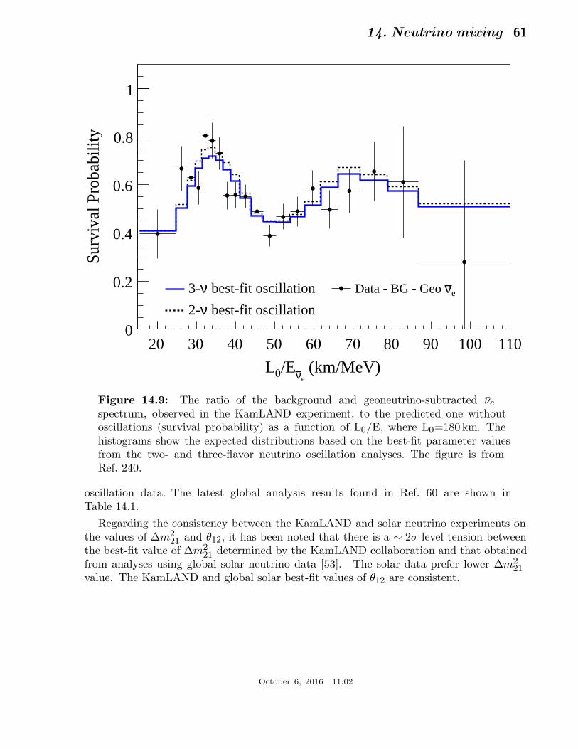
14. Neutrino mixing 61
(km/MeV)eν/E0L
20 30 40 50 60 70 80 90 100 110
Sur
viva
l Pro
babi
lity
0
0.2
0.4
0.6
0.8
1
eνData - BG - Geo best-fit oscillationν3-
best-fit oscillationν2-
Figure 14.9: The ratio of the background and geoneutrino-subtracted νe
spectrum, observed in the KamLAND experiment, to the predicted one withoutoscillations (survival probability) as a function of L0/E, where L0=180 km. Thehistograms show the expected distributions based on the best-fit parameter valuesfrom the two- and three-flavor neutrino oscillation analyses. The figure is fromRef. 240.
oscillation data. The latest global analysis results found in Ref. 60 are shown inTable 14.1.
Regarding the consistency between the KamLAND and solar neutrino experiments onthe values of ∆m2
21 and θ12, it has been noted that there is a ∼ 2σ level tension betweenthe best-fit value of ∆m2
21 determined by the KamLAND collaboration and that obtainedfrom analyses using global solar neutrino data [53]. The solar data prefer lower ∆m2
21value. The KamLAND and global solar best-fit values of θ12 are consistent.
October 6, 2016 11:02
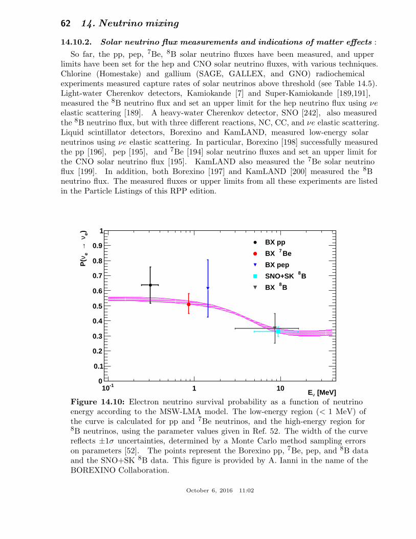
62 14. Neutrino mixing
14.10.2. Solar neutrino flux measurements and indications of matter effects :
So far, the pp, pep, 7Be, 8B solar neutrino fluxes have been measured, and upperlimits have been set for the hep and CNO solar neutrino fluxes, with various techniques.Chlorine (Homestake) and gallium (SAGE, GALLEX, and GNO) radiochemicalexperiments measured capture rates of solar neutrinos above threshold (see Table 14.5).Light-water Cherenkov detectors, Kamiokande [7] and Super-Kamiokande [189,191],measured the 8B neutrino flux and set an upper limit for the hep neutrino flux using νeelastic scattering [189]. A heavy-water Cherenkov detector, SNO [242], also measuredthe 8B neutrino flux, but with three different reactions, NC, CC, and νe elastic scattering.Liquid scintillator detectors, Borexino and KamLAND, measured low-energy solarneutrinos using νe elastic scattering. In particular, Borexino [198] successfully measuredthe pp [196], pep [195], and 7Be [194] solar neutrino fluxes and set an upper limit forthe CNO solar neutrino flux [195]. KamLAND also measured the 7Be solar neutrinoflux [199]. In addition, both Borexino [197] and KamLAND [200] measured the 8Bneutrino flux. The measured fluxes or upper limits from all these experiments are listedin the Particle Listings of this RPP edition.
[MeV]νE-110 1 10
) eν → eν
P(
0
0.1
0.2
0.3
0.4
0.5
0.6
0.7
0.8
0.9
1
BX pp
Be7BX
BX pep
B8SNO+SK
B8BX
Figure 14.10: Electron neutrino survival probability as a function of neutrinoenergy according to the MSW-LMA model. The low-energy region (< 1 MeV) ofthe curve is calculated for pp and 7Be neutrinos, and the high-energy region for8B neutrinos, using the parameter values given in Ref. 52. The width of the curvereflects ±1σ uncertainties, determined by a Monte Carlo method sampling errorson parameters [52]. The points represent the Borexino pp, 7Be, pep, and 8B dataand the SNO+SK 8B data. This figure is provided by A. Ianni in the name of theBOREXINO Collaboration.
October 6, 2016 11:02

14. Neutrino mixing 63
Fig. 14.10 plots the survival probability of solar νe as a function of neutrino energy.The data points are from the Borexino results except the SNO+SK 8B data. As explainedin Section 14.8.2.2, matter effects on solar neutrino oscillation is expected to be given bythe average two-neutrino vacuum oscillation probability, 1 − 1
2sin22θ12 for survival of pp
neutrinos. It is ∼ 0.58 for sin2θ12 = 0.297. For 8B neutrinos, transitions are adiabatic andthe survival probability is given by sin4θ13 + cos4θ13 sin2θ12 ∼ 0.28 for sin2θ13 = 0.0214(for normal mass ordering) and sin2θ12 = 0.297. All the data shown in this plot areconsistent with the theoretically calculated curve. This indicates that these solar neutrinoresults are consistent with the MSW-LMA solution of the solar neutrino problem.
In the nighttime, solar neutrino experiments observe neutrinos propagated throughthe Earth. Therefore, a non-zero day-night flux (or interaction rate) asymmetry impliesthe Earth matter effects on flavour oscillations of solar neutrinos. In particular, if thenighttime flux is higher than the daytime flux, it implies a νe regeneration by the Earthmatter effects (see Section 14.8.2.3). Previously, SNO [242] and Borexino [243] searchedfor day-night flux asymmetries of 8B and 7Be neutrinos, respectively, but they observedno statistically significant asymmetries. Recently, the Super-Kamiokande experiment hasreported [244] a 2.7 σ indication of non-zero day-night asymmetry of 8B solar neutrinos,ADN = 2(RD − RN )/(RD + RN ) = −0.032 ± 0.011 ± 0.005, where RD and RN are theaverage day and average night νe elastic-scattering rates of 8B solar neutrinos. Thisresult is consistent with the ∆m2
21 and θ12 values in the LMA region.
14.11. Measurements of |∆m231(32)| and θ23, and related topics
The first compelling evidence for the neutrino oscillation was νµ disappearanceobserved by the Super-Kamiokande Collaboration in 1998 [17] in the measurement ofatmospheric neutrinos produced by cosmic-ray interactions in the atmosphere. A strikingfeature of atmospheric neutrino oscillations was a surprisingly large mixing angle θ23.Whether mixing is maximal, i.e., θ23 = π/4, or, if not, in which octant θ23 lies, is oneof the questions drawing much interest in neutrino physics because the measurementof certain fundamental physical observables depends on the value of sin2 θ23 (see, e.g.,Sections 14.2 and 14.8.1). The high precision measurement of sin2 θ23 will provide also atest of a large class of theories of neutrino masses and mixing, based, in particular, ondiscrete symmetries (see, e.g., the first two articles quoted in Ref. 87 and Ref. 245).
14.11.1. νµ disappearance :
Prior to the Super-Kamiokande’s discovery of atmospheric neutrino oscillations, adeficit of atmospheric νµ + νµ flux was indicated by the Kamiokande experiment [204].Actually, Kamiokande reported the double ratio R(νµ/νe) = (Measured νµ/νe)/(Expectedνµ/νe)< 1 to reduce systematic effects due to rather large flux uncertainties. TheIMB [206] and Soudan 2 [208] experiments also observed R < 1, but the Frejusexperiment [207] did not see such a tendency. Kamiokande further observed zenith-dependence of νµ + νµ flux deficit [205]. However, all these results from early experimentsdid not have conclusive statistical significance.
In 1998, the Super-Kamiokande Collaboration reported a significant zenith-angle (Θ)dependent deficit of µ-like events compared to the no-oscillation expectation [17]. For
October 6, 2016 11:02
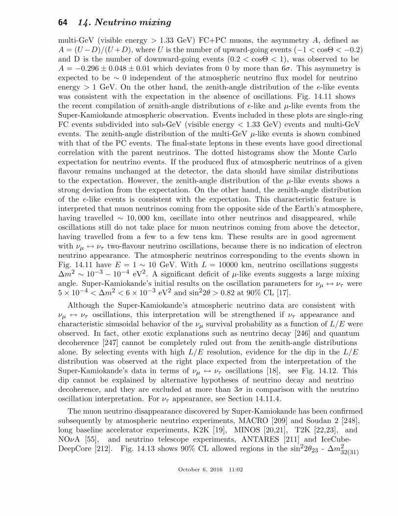
64 14. Neutrino mixing
multi-GeV (visible energy > 1.33 GeV) FC+PC muons, the asymmetry A, defined asA = (U−D)/(U +D), where U is the number of upward-going events (−1 < cosΘ < −0.2)and D is the number of downward-going events (0.2 < cosΘ < 1), was observed to beA = −0.296 ± 0.048 ± 0.01 which deviates from 0 by more than 6σ. This asymmetry isexpected to be ∼ 0 independent of the atmospheric neutrino flux model for neutrinoenergy > 1 GeV. On the other hand, the zenith-angle distribution of the e-like eventswas consistent with the expectation in the absence of oscillations. Fig. 14.11 showsthe recent compilation of zenith-angle distributions of e-like and µ-like events from theSuper-Kamiokande atmospheric observation. Events included in these plots are single-ringFC events subdivided into sub-GeV (visible energy < 1.33 GeV) events and multi-GeVevents. The zenith-angle distribution of the multi-GeV µ-like events is shown combinedwith that of the PC events. The final-state leptons in these events have good directionalcorrelation with the parent neutrinos. The dotted histograms show the Monte Carloexpectation for neutrino events. If the produced flux of atmospheric neutrinos of a givenflavour remains unchanged at the detector, the data should have similar distributionsto the expectation. However, the zenith-angle distribution of the µ-like events shows astrong deviation from the expectation. On the other hand, the zenith-angle distributionof the e-like events is consistent with the expectation. This characteristic feature isinterpreted that muon neutrinos coming from the opposite side of the Earth’s atmosphere,having travelled ∼ 10, 000 km, oscillate into other neutrinos and disappeared, whileoscillations still do not take place for muon neutrinos coming from above the detector,having travelled from a few to a few tens km. These results are in good agreementwith νµ ↔ ντ two-flavour neutrino oscillations, because there is no indication of electronneutrino appearance. The atmospheric neutrinos corresponding to the events shown inFig. 14.11 have E = 1 ∼ 10 GeV. With L = 10000 km, neutrino oscillations suggests∆m2 ∼ 10−3 − 10−4 eV2. A significant deficit of µ-like events suggests a large mixingangle. Super-Kamiokande’s initial results on the oscillation parameters for νµ ↔ ντ were5 × 10−4 < ∆m2 < 6 × 10⁻³ eV2 and sin22θ > 0.82 at 90% CL [17].
Although the Super-Kamiokande’s atmospheric neutrino data are consistent withνµ ↔ ντ oscillations, this interpretation will be strengthened if ντ appearance andcharacteristic sinusoidal behavior of the νµ survival probability as a function of L/E wereobserved. In fact, other exotic explanations such as neutrino decay [246] and quantumdecoherence [247] cannot be completely ruled out from the zenith-angle distributionsalone. By selecting events with high L/E resolution, evidence for the dip in the L/Edistribution was observed at the right place expected from the interpretation of theSuper-Kamiokande’s data in terms of νµ ↔ ντ oscillations [18], see Fig. 14.12. Thisdip cannot be explained by alternative hypotheses of neutrino decay and neutrinodecoherence, and they are excluded at more than 3σ in comparison with the neutrinooscillation interpretation. For ντ appearance, see Section 14.11.4.
The muon neutrino disappearance discovered by Super-Kamiokande has been confirmedsubsequently by atmospheric neutrino experiments, MACRO [209] and Soudan 2 [248],long baseline accelerator experiments, K2K [19], MINOS [20,21], T2K [22,23], andNOνA [55], and neutrino telescope experiments, ANTARES [211] and IceCube-DeepCore [212]. Fig. 14.13 shows 90% CL allowed regions in the sin22θ23 - ∆m2
32(31)
October 6, 2016 11:02
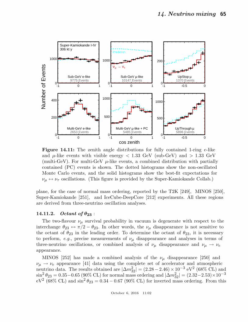
14. Neutrino mixing 65
cos zenith
Num
ber
of E
vent
s
-1 0 10
1000
Sub-GeV e-like 9775 Events
Super-Kamiokande I-IV306 kt y
-1 0 10
1000
-likeµSub-GeV 10147 Events
Prediction
τν → µν
-1 -0.5 00
200
µUpStop 1370 Events
-1 0 10
200
400
Multi-GeV e-like 2653 Events
-1 0 10
500
1000
-like + PCµMulti-GeV 5485 Events
-1 -0.5 00
500
1000
µUpThrough 5896 Events
Figure 14.11: The zenith angle distributions for fully contained 1-ring e-likeand µ-like events with visible energy < 1.33 GeV (sub-GeV) and > 1.33 GeV(multi-GeV). For multi-GeV µ-like events, a combined distribution with partiallycontained (PC) events is shown. The dotted histograms show the non-oscillatedMonte Carlo events, and the solid histograms show the best-fit expectations forνµ ↔ ντ oscillations. (This figure is provided by the Super-Kamiokande Collab.)
plane, for the case of normal mass ordering, reported by the T2K [249], MINOS [250],Super-Kamiokande [251], and IceCube-DeepCore [212] experiments. All these regionsare derived from three-neutrino oscillation analyses.
14.11.2. Octant of θ23 :
The two-flavour νµ survival probability in vacuum is degenerate with respect to theinterchange θ23 ↔ π/2 − θ23. In other words, the νµ disappearance is not sensitive tothe octant of θ23 in the leading order. To determine the octant of θ23, it is necessaryto perform, e.g., precise measurements of νµ disappearance and analyses in terms ofthree-neutrino oscillations, or combined analysis of νµ disappearance and νµ → νe
appearance.
MINOS [252] has made a combined analysis of the νµ disappearance [250] andνµ → νe appearance [41] data using the complete set of accelerator and atmosphericneutrino data. The results obtained are |∆m2
32| = (2.28− 2.46)× 10−3 eV2 (68% CL) andsin2 θ23 = 0.35−0.65 (90% CL) for normal mass ordering and |∆m2
32| = (2.32−2.53)×10−3
eV2 (68% CL) and sin2 θ23 = 0.34− 0.67 (90% CL) for inverted mass ordering. From this
October 6, 2016 11:02
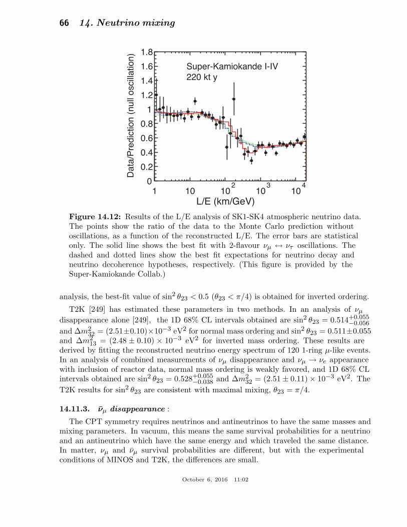
66 14. Neutrino mixing
0
0.2
0.4
0.6
0.8
1
1.2
1.4
1.6
1.8
1 10 102
103
104
L/E (km/GeV)
Super-Kamiokande I-IV
220 kt y
Da
ta/P
red
ictio
n (
nu
ll o
scill
atio
n)
Figure 14.12: Results of the L/E analysis of SK1-SK4 atmospheric neutrino data.The points show the ratio of the data to the Monte Carlo prediction withoutoscillations, as a function of the reconstructed L/E. The error bars are statisticalonly. The solid line shows the best fit with 2-flavour νµ ↔ ντ oscillations. Thedashed and dotted lines show the best fit expectations for neutrino decay andneutrino decoherence hypotheses, respectively. (This figure is provided by theSuper-Kamiokande Collab.)
analysis, the best-fit value of sin2 θ23 < 0.5 (θ23 < π/4) is obtained for inverted ordering.
T2K [249] has estimated these parameters in two methods. In an analysis of νµ
disappearance alone [249], the 1D 68% CL intervals obtained are sin2 θ23 = 0.514+0.055−0.056
and ∆m232 = (2.51±0.10)×10−3 eV2 for normal mass ordering and sin2 θ23 = 0.511±0.055
and ∆m213 = (2.48 ± 0.10) × 10−3 eV2 for inverted mass ordering. These results are
derived by fitting the reconstructed neutrino energy spectrum of 120 1-ring µ-like events.In an analysis of combined measurements of νµ disappearance and νµ → νe appearancewith inclusion of reactor data, normal mass ordering is weakly favored, and 1D 68% CLintervals obtained are sin2 θ23 = 0.528+0.055
−0.038 and ∆m232 = (2.51 ± 0.11) × 10−3 eV2. The
T2K results for sin2 θ23 are consistent with maximal mixing, θ23 = π/4.
14.11.3. νµ disappearance :
The CPT symmetry requires neutrinos and antineutrinos to have the same masses andmixing parameters. In vacuum, this means the same survival probabilities for a neutrinoand an antineutrino which have the same energy and which traveled the same distance.In matter, νµ and νµ survival probabilities are different, but with the experimentalconditions of MINOS and T2K, the differences are small.
October 6, 2016 11:02
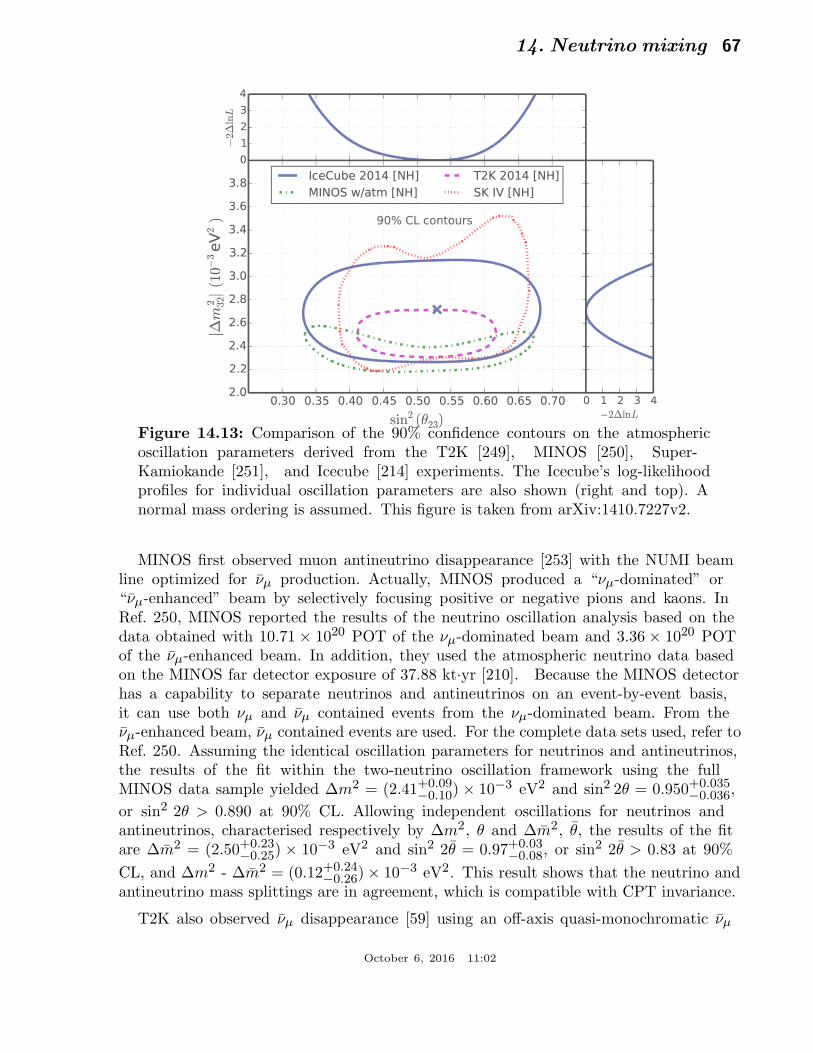
14. Neutrino mixing 67
Figure 14.13: Comparison of the 90% confidence contours on the atmosphericoscillation parameters derived from the T2K [249], MINOS [250], Super-Kamiokande [251], and Icecube [214] experiments. The Icecube’s log-likelihoodprofiles for individual oscillation parameters are also shown (right and top). Anormal mass ordering is assumed. This figure is taken from arXiv:1410.7227v2.
MINOS first observed muon antineutrino disappearance [253] with the NUMI beamline optimized for νµ production. Actually, MINOS produced a “νµ-dominated” or“νµ-enhanced” beam by selectively focusing positive or negative pions and kaons. InRef. 250, MINOS reported the results of the neutrino oscillation analysis based on thedata obtained with 10.71 × 10²⁰ POT of the νµ-dominated beam and 3.36 × 10²⁰ POTof the νµ-enhanced beam. In addition, they used the atmospheric neutrino data basedon the MINOS far detector exposure of 37.88 kt·yr [210]. Because the MINOS detectorhas a capability to separate neutrinos and antineutrinos on an event-by-event basis,it can use both νµ and νµ contained events from the νµ-dominated beam. From theνµ-enhanced beam, νµ contained events are used. For the complete data sets used, refer toRef. 250. Assuming the identical oscillation parameters for neutrinos and antineutrinos,the results of the fit within the two-neutrino oscillation framework using the fullMINOS data sample yielded ∆m2 = (2.41+0.09
−0.10) × 10−3 eV2 and sin2 2θ = 0.950+0.035−0.036,
or sin2 2θ > 0.890 at 90% CL. Allowing independent oscillations for neutrinos andantineutrinos, characterised respectively by ∆m2, θ and ∆m2, θ, the results of the fitare ∆m2 = (2.50+0.23
−0.25) × 10−3 eV2 and sin2 2θ = 0.97+0.03−0.08, or sin2 2θ > 0.83 at 90%
CL, and ∆m2 - ∆m2 = (0.12+0.24−0.26) × 10−3 eV2. This result shows that the neutrino and
antineutrino mass splittings are in agreement, which is compatible with CPT invariance.
T2K also observed νµ disappearance [59] using an off-axis quasi-monochromatic νµ
October 6, 2016 11:02
68 14. Neutrino mixing
beam peaked at ∼ 0.6 GeV with the polarity of the horn current set to focus negativepions. With 4.01 × 10²⁰ POT, 34 fully contained µ-like events were observed at theSuper-Kamiokande. Oscillation parameters sin2 θ23 and ∆m2
32 are estimated in thethree-neutrino oscillation framework assuming the normal mass ordering, and all otherparameters fixed to the values taken from the previous T2K fits [57] and Review ofParticle Properties [103]. The best-fit parameters obtained are ∆m2
32 = 2.51 × 10⁻³
eV2 and sin2 θ23 = 0.45, with 68% confidence intervals of (2.26 − 2.80) × 10−3 eV2 for∆m2
32 and 0.38 - 0.64 for sin2 θ23. These results are consistent with the MINOS νµ
disappearance results [253] as well as the νµ disappearance parameters measured byT2K [57].
14.11.4. ντ appearance :
Super-Kamiokande Collaboration searched for the appearance of τ leptons from theCC interactions of oscillation-generated ντ in the detector using the atmospheric neutrinodata [254,24]. An excess of τ -like events is expected in the upward-going direction.Though the Super-Kamiokande detector cannot identify a CC ντ interaction on an eventby event basis, the Super-Kamiokande Collaboration excluded the no-tau-appearancehypothesis at the 3.8σ level through a neural network analysis on the zenith-angledistribution of multi-GeV contained events [24].
For the purpose of demonstrating the appearance of tau neutrinos on an event-by-eventbasis, a promising method is an accelerator long-baseline experiment using emulsiontechnique to identify short-lived τ leptons produced in the ντ CC interactions. OPERAadopted this strategy and searched for the appearance of ντ in the CNGS muon neutrinobeam during 2008 and 2012, corresponding to a live exposure of 17.97 × 10¹⁹ POT intotal. In 2010, OPERA reported observation of the first ντ candidate [141]. As of July2015, OPERA has reported observation of the fifth ντ candidate [255]. The observedcandidate events are classified into the four decay channels, τ → 1h (hadronic 1-prong),τ → 1h (hadronic 3-prong), τ → µ, and τ → e, and expected signal and backgroundevents are calculated for each decay channel. The expected total signal and backgroundevents are, respectively, 2.64± 0.53 and 0.25± 0.05. With 5 events observed, the OPERACollaboration concludes the discovery of ντ appearance with a significance larger than 5σ.
14.12. Measurements of θ13
In 2012, the last neutrino mixing angle θ13 was established to be non-zero by reactorexperiments. The measured value of θ13 was sufficiently large to widen the opportunitiesto measure the unknown CP-violating phase δ in the PMNS matrix and the neutrinomass ordering.
October 6, 2016 11:02
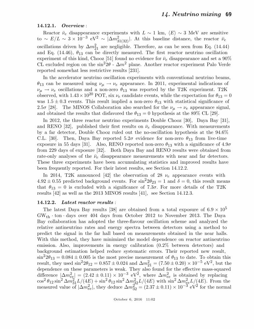
14. Neutrino mixing 69
14.12.1. Overview :
Reactor νe disappearance experiments with L ∼ 1 km, 〈E〉 ∼ 3 MeV are sensitiveto ∼ E/L ∼ 3 × 10⁻³ eV2 ∼ |∆m2
31(32)|. At this baseline distance, the reactor νe
oscillations driven by ∆m221 are negligible. Therefore, as can be seen from Eq. (14.44)
and Eq. (14.46), θ13 can be directly measured. The first reactor neutrino oscillationexperiment of this kind, Chooz [51] found no evidence for νe disappearance and set a 90%CL excluded region on the sin22θ - ∆m2 plane. Another reactor experiment Palo Verdereported somewhat less restrictive results [231].
In the accelerator neutrino oscillation experiments with conventional neutrino beams,θ13 can be measured using νµ → νe appearance. In 2011, experimental indications ofνµ → νe oscillations and a non-zero θ13 was reported by the T2K experiment. T2Kobserved, with 1.43×10²⁰ POT, six νe candidate events, while the expectation for θ13 = 0was 1.5 ± 0.3 events. This result implied a non-zero θ13 with statistical significance of2.5σ [28]. The MINOS Collaboration also searched for the νµ → νe appearance signal,and obtained the results that disfavored the θ13 = 0 hypothesis at the 89% CL [29].
In 2012, the three reactor neutrino experiments Double Chooz [30], Daya Bay [31],and RENO [32], published their first results on νe disappearance. With measurementsby a far detector, Double Chooz ruled out the no-oscillation hypothesis at the 94.6%C.L. [30]. Then, Daya Bay reported 5.2σ evidence for non-zero θ13 from live-timeexposure in 55 days [31]. Also, RENO reported non-zero θ13 with a significance of 4.9σfrom 229 days of exposure [32]. Both Daya Bay and RENO results were obtained fromrate-only analyses of the νe disappearance measurements with near and far detectors.These three experiments have been accumulating statistics and improved results havebeen frequently reported. For their latest results, see Section 14.12.2.
In 2014, T2K announced [42] the observation of 28 νe appearance events with4.92 ± 0.55 predicted background events. For sin22θ23 = 1 and δ = 0, this result meansthat θ13 = 0 is excluded with a significance of 7.3σ. For more details of the T2Kresults [42] as well as the 2013 MINOS results [41], see Section 14.12.3.
14.12.2. Latest reactor results :
The latest Daya Bay results [38] are obtained from a total exposure of 6.9 × 10⁵
GWth · ton · days over 404 days from October 2012 to November 2013. The DayaBay collaboration has adopted the three-flavour oscillation scheme and analyzed therelative antineutrino rates and energy spectra between detectors using a method topredict the signal in the far hall based on measurements obtained in the near halls.With this method, they have minimized the model dependence on reactor antineutrinoemission. Also, improvements in energy calibration (0.2% between detectors) andbackground estimation helped reduce systematic errors. Their reported new result,sin22θ13 = 0.084 ± 0.005 is the most precise measurement of θ13 to date. To obtain thisresult, they used sin22θ12 = 0.857± 0.024 and ∆m2
21 = (7.50± 0.20)× 10−5 eV2, but thedependence on these parameters is weak. They also found for the effective mass-squareddifference |∆m2
ee| = (2.42 ± 0.11) × 10−3 eV2, where ∆m2ee is obtained by replacing
cos2 θ12 sin2 ∆m231L/(4E) + sin2 θ12 sin2 ∆m2
32L/(4E) with sin2 ∆m2eeL/(4E). From the
measured value of |∆m2ee|, they deduce ∆m2
32 = (2.37 ± 0.11) × 10−3 eV2 for the normal
October 6, 2016 11:02
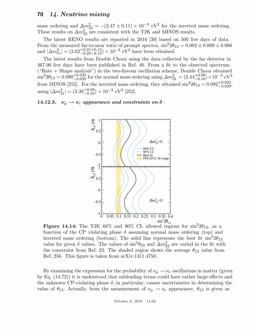
70 14. Neutrino mixing
mass ordering and ∆m232 = −(2.47 ± 0.11) × 10−3 eV2 for the inverted mass ordering.
These results on ∆m232 are consistent with the T2K and MINOS results.
The latest RENO results are reported in 2016 [39] based on 500 live days of data.From the measured far-to-near ratio of prompt spectra, sin22θ13 = 0.082 ± 0.009 ± 0.006and |∆m2
ee| = (2.62+0.21+0.12−0.23−0.13) × 10−3 eV2 have been obtained.
The latest results from Double Chooz using the data collected by the far detector in467.90 live days have been published in Ref. 40. From a fit to the observed spectrum(“Rate + Shape analysis”) in the two-flavour oscillation scheme, Double Chooz obtainedsin22θ13 = 0.090+0.032
−0.029 for the normal mass ordering using ∆m231 = (2.44+0.09
−0.10)×10−3 eV2
from MINOS [252]. For the inverted mass ordering, they obtained sin22θ13 = 0.092+0.033−0.029,
using |∆m231| = (2.38+0.09
−0.10) × 10−3 eV2 [252].
14.12.3. νµ → νe appearance and constraints on δ :
)π (
CP
δ
68% CL90% CLBest fit
rangeσPDG2012 1
>0322m∆
-1
-0.5
0
0.5
1
13θ22sin0 0.05 0.1 0.15 0.2 0.25 0.3 0.35 0.4
)π (
CP
δ
<0322m∆
-1
-0.5
0
0.5
1
Figure 14.14: The T2K 68% and 90% CL allowed regions for sin22θ13, as afunction of the CP violating phase δ assuming normal mass ordering (top) andinverted mass ordering (bottom). The solid line represents the best fit sin22θ13
value for given δ values. The values of sin2θ23 and ∆m232 are varied in the fit with
the constraint from Ref. 23. The shaded region shows the average θ13 value fromRef. 256. This figure is taken from arXiv:1311.4750.
By examining the expression for the probability of νµ → νe oscillations in matter (givenby Eq. (14.72)) it is understood that subleading terms could have rather large effects andthe unknown CP-violating phase δ, in particular, causes uncertainties in determining thevalue of θ13. Actually, from the measurement of νµ → νe appearance, θ13 is given as
October 6, 2016 11:02
14. Neutrino mixing 71
)π (CPδ-1 -0.5 0 0.5 1
lnL
∆-2
0
1
2
3
4
5
6>032
2m∆<032
2m∆>0)32
2m∆90% CL (
<0)322m∆90% CL (
Figure 14.15: The T2K value of −2∆ lnL as a function of the CP violating phase δfor normal mass ordering (solid line) and inverted mass ordering (dotted line). Thelikelihood is marginalized over sin22θ13, sin2θ23 and ∆m2
32. The solid (dotted) linewith markers corresponds to the 90% CL limits for normal (inverted) mass ordering,evaluated by using the Feldman-Cousins method. The δ regions with values abovethe lines are excluded at 90% CL. This figure is taken from arXiv:1311.4750.
a function of δ for a given sign and value of ∆m231, and values of θ23, ∆m2
21 and θ12.Therefore, a single experiment with a neutrino beam cannot determine the value of θ13,although it is possible to establish a non-zero θ13. On the other hand, a combination ofthe νµ → νe appearance results and the precise measurements of θ13 from the reactorexperiments can yield constraints on the possible value of δ.
In Ref. 42, with the observation of 28 νe appearance events with 4.92 ± 0.55 predictedbackground events, for δ = 0, sin2 θ23 = 0.5 and |∆m2
31(32)| = 2.4 × 10⁻³eV2, the T2K
collaborations finds in the case of ∆m231(32)
> 0 (∆m231(32)
< 0): sin2 2θ13 = 0.140+0.038−0.032
(0.170+0.045−0.037). The significance of nonzero θ13 is 7.3σ for these fixed values of θ23 and
δ. Changing the values of θ23 and δ within uncertainties, the significance remains above7σ. The best fit value of sin2 2θ13 thus found in the T2K experiment is approximatelyby a factor of 1.6 (1.9) bigger than that found in the Daya Bay experiment [36]. Thisimplies that the compatibility of the results of the two experiments on sin2 2θ13 requires,in particular, that δ 6= 0 and/or sin2 θ23 6= 0.5. As we have seen in Section 14.2, theindicated results lead to a certain indication about the possible value of δ in the globalanalyses of the neutrino oscillation data. T2K has also calculated the 68% and 90% CLallowed regions for sin22θ13, as a function of δ. The results are shown in Fig. 14.14 wherethe 1σ range of the sin22θ13 value from reactor experiments is also shown. T2K has
October 6, 2016 11:02
72 14. Neutrino mixing
further calculated constraints on δ by combining the νµ → νe appearance results withthe θ13 value from reactor experiments into a likelihood function L. Fig. 14.15 shows the−2∆ lnL value as a function of δ. From this figure, it is seen that the combined T2K andreactor measurements prefer δ = −π/2 or 3π/2 for both the normal and inverted massordering, and some δ regions are excluded at 90% CL.
In Ref. 41, MINOS has extended the analysis using 10.6 × 10²⁰ POT ν-beammode and 3.3 × 10²⁰ POT ν-beam mode appearance data. Assuming ∆m2
31(32)> 0
(∆m231(32)
< 0), δ = 0, and θ23 < π/4, the results of this analysis imply that
0.01 (0.03) < 2 sin2θ23 sin22θ13 < 0.12 (0.18) at the 90% CL, with the best fit value 2sin2θ23 sin22θ13 = 0.051+0.038
−0.030 (0.093+0.054−0.049). MINOS has also placed constraints on the
value of δ by combining the full MINOS appearance data and the reactor measurementsof θ13.
In 2016, NOνA reported its first result of νe appearance measurement [56]. Thedata were taken between February 2014 and May 2015. During this period, the effectivefiducial mass of the NOνA far detector varied from 2.3 kt for 4.0 kt of total mass to 10 ktfor the full 14 kt. The exposure corresponding to these data is equivalent to 2.74 × 10²⁰
POT collected in the full 14 kt far detector, and 6 νe-like events were observed comparedto 0.99 ± 0.11 (syst.) expected background events: a 3.3σ excess over the backgroundprediction. NOνA also quote the result of a secondary event selection method. With thisanalysis, 11 events were observed over the expected background of 1.07 ± 0.14 (syst.)events.
14.13. Search for Oscillations Involving Light Sterile Neutrinos
Although the mixing of the 3 flavour neutrino states has been experimentally wellestablished, implying the existence of 3 light neutrinos νj having masses mj not exceedingapproximately 1 eV, there have been possible hints for the presence in the mixing ofone or more additional neutrino states with masses at the eV scale. If these states exist,they must be related to the existence of one or more sterile neutrinos (sterile neutrinofields) which mix with the active flavour neutrinos (active flavour neutrino fields).The hints under discussion have been obtained: i) in the LSND νµ → νe appearanceexperiment [225], in which a significant excess of events over the background is claimedto have been observed, ii) from the analysis of the νµ → νe [228] and νµ → νe [227]appearance data of the MiniBooNE experiment, iii) from the re-analyses of the shortbaseline (SBL) reactor neutrino oscillation data using newly calculated fluxes of reactorνe [257,119], which show a possible “disappearance” of the reactor νe (“reactorneutrino anomaly”), and iv) from the data of the radioactive source calibrations of theGALLEX [202] and SAGE [203] solar neutrino experiments.
The short baseline neutrino oscillation experiment MiniBooNE at Fermilab investigatedνe [227] and νe [228] appearance in νµ and νµ beams, respectively, with a detectorcontaining 800 tons of mineral oil and located 541 m downstream of the production target.With the antineutrino running mode [228], a 2.8σ excess of events over the backgroundwas observed in the energy range of 200 < Eν < 1250 MeV in the charged-currentquasielastic data. Excess events were observed, in particular, in the interval of energies
October 6, 2016 11:02

14. Neutrino mixing 73
200 < Eν < 475 MeV, which corresponds to L/E range outside of that probed in theLSND experiment. The origin of this excess is not understood. Employing a simple2-neutrino oscillation hypothesis and using the data from the entire neutrino energyinterval 200 < Eν < 1250 MeV used in the data analysis, this result, interpreted in termsof νµ → νe oscillations, corresponds to an allowed region in the sin2 2θ − ∆m2 plane,which overlaps with the allowed region obtained from the interpretation of the LSND datain terms of νµ → νe oscillations. The overlap region at the 90% CL extends over ∆m2 ∼a few ×10−2 eV2 at sin22θ = 1 to 1 eV2 at sin22θ = a few ×10−3. The MiniBooNECollaboration studied also the CP conjugate oscillation channel [227], νµ → νe, andobserved a 3.4 σ excess of events in the same energy range. Most of the excess events liein the interval 200 < Eν < 475 MeV and are incompatible with the νµ → νe oscillationinterpretation of the LSND data. The energy spectra of the excess events observed in theνµ [227] and νµ [228] runs are only marginally compatible with each other and thus withthe simple 2-neutrino oscillation hypothesis.
The reactor neutrino anomaly [257] is related to the results of a new and very detailedcalculation of the reactor νe fluxes [119] which were found to be by approximately3.5% larger than the fluxes calculated in Ref. 122 and widely used in the past in theinterpretation of the data of the SBL reactor νe oscillation experiments. These data showindications for reactor νe “disappearance” when analyzed using the fluxes from [119].It should be added that there are a number of uncertainties in the calculation of thefluxes under discussion (associated, e.g., with the weak magnetism term contribution tothe corresponding β-decay rates [120], the contribution of a relatively large number of“forbidden” β-decays [258], etc.) which can be of the order of the difference between the“old” and “new” fluxes.
Radioactive source calibrations of the GALLEX [202] and SAGE [203] experimentsalso showed a deficit of the measured fluxes compared to the expected fluxes (“Galliumanomaly”), and therefore might be interpreted as hints for νe disappearance.
Significant constraints on the parameters characterizing the oscillations involving sterileneutrinos follow from the negative results of the searches for νµ → νe and/or νµ → νe
oscillations in the Karmen [226], NOMAD [259], ICARUS [224], and OPERA [260]experiments, and from the nonobservation of effects of oscillations into sterile neutrinosin the solar neutrino experiments and in the studies of νµ and/or νµ disappearance in theCDHSW [261], MINOS and SuperKamiokande experiments.
Two possible “minimal” phenomenological models (or schemes) with light sterileneutrinos are widely used in order to explain the data discussed in this section in terms ofneutrino oscillations: the so-called “3 + 1” and “3 + 2” models. They contain respectivelyone and two sterile neutrinos (right-handed sterile neutrino fields). Thus, the “3 + 1” and“3 + 2” models have altogether 4 and 5 light massive neutrinos νj , which in the minimalversions of these models are Majorana particles. The additional neutrinos ν4 and ν4, ν5
should have masses m4 and m4, m5 at the eV scale (see below). It follows from the datathat if ν4 or ν4, ν5 exist, they couple to the electron and muon in the weak charged leptoncurrent with couplings Uek and Uµk, k = 4; 4, 5, which are approximately |Uek| ∼ 0.1and |Uµk| ∼ 0.1.
Global analysis of all the data (positive evidences and negative results) relevant for
October 6, 2016 11:02
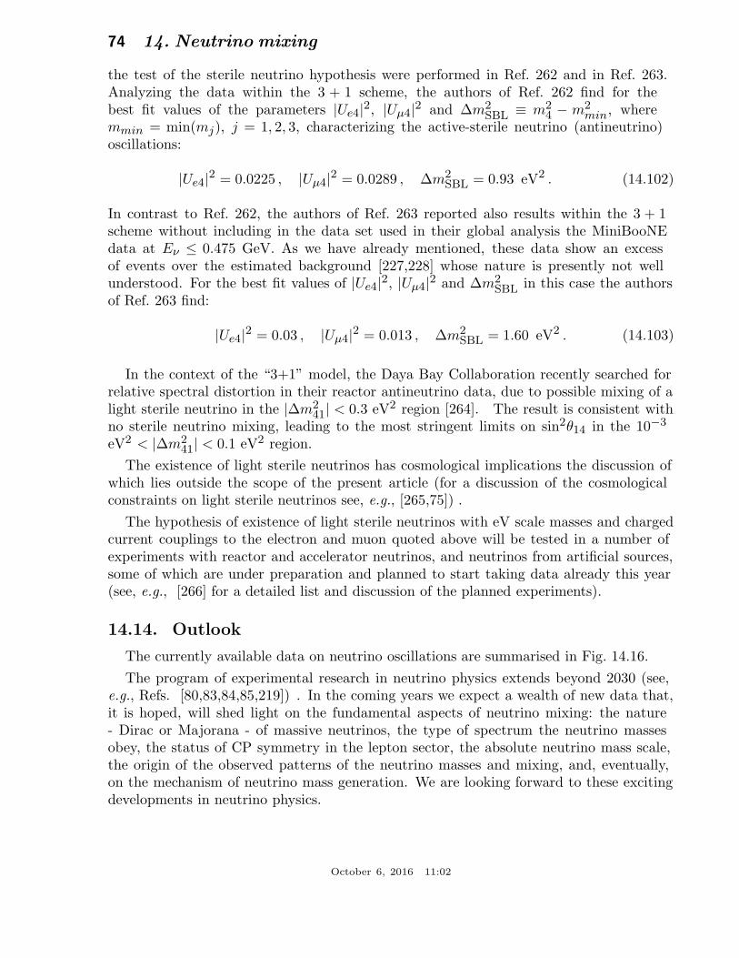
74 14. Neutrino mixing
the test of the sterile neutrino hypothesis were performed in Ref. 262 and in Ref. 263.Analyzing the data within the 3 + 1 scheme, the authors of Ref. 262 find for thebest fit values of the parameters |Ue4|2, |Uµ4|2 and ∆m2
SBL ≡ m24 − m2
min, wheremmin = min(mj), j = 1, 2, 3, characterizing the active-sterile neutrino (antineutrino)oscillations:
|Ue4|2 = 0.0225 , |Uµ4|2 = 0.0289 , ∆m2SBL = 0.93 eV2 . (14.102)
In contrast to Ref. 262, the authors of Ref. 263 reported also results within the 3 + 1scheme without including in the data set used in their global analysis the MiniBooNEdata at Eν ≤ 0.475 GeV. As we have already mentioned, these data show an excessof events over the estimated background [227,228] whose nature is presently not wellunderstood. For the best fit values of |Ue4|2, |Uµ4|2 and ∆m2
SBL in this case the authorsof Ref. 263 find:
|Ue4|2 = 0.03 , |Uµ4|2 = 0.013 , ∆m2SBL = 1.60 eV2 . (14.103)
In the context of the “3+1” model, the Daya Bay Collaboration recently searched forrelative spectral distortion in their reactor antineutrino data, due to possible mixing of alight sterile neutrino in the |∆m2
41| < 0.3 eV2 region [264]. The result is consistent withno sterile neutrino mixing, leading to the most stringent limits on sin2θ14 in the 10−3
eV2 < |∆m241| < 0.1 eV2 region.
The existence of light sterile neutrinos has cosmological implications the discussion ofwhich lies outside the scope of the present article (for a discussion of the cosmologicalconstraints on light sterile neutrinos see, e.g., [265,75]) .
The hypothesis of existence of light sterile neutrinos with eV scale masses and chargedcurrent couplings to the electron and muon quoted above will be tested in a number ofexperiments with reactor and accelerator neutrinos, and neutrinos from artificial sources,some of which are under preparation and planned to start taking data already this year(see, e.g., [266] for a detailed list and discussion of the planned experiments).
14.14. Outlook
The currently available data on neutrino oscillations are summarised in Fig. 14.16.
The program of experimental research in neutrino physics extends beyond 2030 (see,e.g., Refs. [80,83,84,85,219]) . In the coming years we expect a wealth of new data that,it is hoped, will shed light on the fundamental aspects of neutrino mixing: the nature- Dirac or Majorana - of massive neutrinos, the type of spectrum the neutrino massesobey, the status of CP symmetry in the lepton sector, the absolute neutrino mass scale,the origin of the observed patterns of the neutrino masses and mixing, and, eventually,on the mechanism of neutrino mass generation. We are looking forward to these excitingdevelopments in neutrino physics.
October 6, 2016 11:02
14. Neutrino mixing 75
Super-K
95%
all solar 95%
KamLAND
95%
Borexino
95%
Cl 95%
Ga 95%
νµ↔ν
τ
νe↔ν
X
100
10–3
∆m
2 [
eV
2]
10–12
10–9
10–6
10210010–210–4
tan2θ
KA
RM
EN
2
νe↔ν
τνe↔ν
µ
SNO
95%
All limits are at 90%CL
unless otherwise noted
Normal hierarchy assumed
whenever relevant
CHOOZK2K
Bugey
CHORUSNOMAD
CHORUS
NOMAD
CDHSW
NOMAD
LSND 90/99%
MiniBooNE
OPERA
ICARUS
Daya Bay 95%T2K
RENO 95%Super-K
MINOST2K
NOνAIceCube
Figure 14.16: The regions of squared-mass splitting and mixing angle favored orexcluded by various neutrino oscillation experiments. The figure was contributed byH. Murayama (University of California, Berkeley, and Kavli IPMU, University ofTokyo). References to the data used in the figure and the description of how thefigure was obtained can be found at http://hitoshi.berkeley.edu/neutrino.
October 6, 2016 11:02
76 14. Neutrino mixing
References:
1. B. Pontecorvo, Zh. Eksp. Teor. Fiz. 53, 1717 (1967) [Sov. Phys. JETP 26, 984(1968)].
2. M. Fukugita and T. Yanagida, Phys. Lett. B174, 45 (1986); V.A. Kuzmin,V.A. Rubakov, and M.E. Shaposhnikov, Phys. Lett. B155, 36 (1985).
3. P. Minkowski, Phys. Lett. B67, 421 (1977); see also: M. Gell-Mann, P. Ramond,and R. Slansky in Supergravity, p. 315, edited by F. Nieuwenhuizen andD. Friedman, North Holland, Amsterdam, 1979; T. Yanagida, Proc. of theWorkshop on Unified Theories and the Baryon Number of the Universe, editedby O. Sawada and A. Sugamoto, KEK, Japan 1979; R.N. Mohapatra andG. Senjanovic, Phys. Rev. Lett. 44, 912 (1980).
4. B. Pontecorvo, Zh. Eksp. Teor. Fiz. 33, 549 (1957) and 34, 247 (1958).5. Z. Maki, M. Nakagawa, and S. Sakata, Prog. Theor. Phys. 28, 870 (1962).6. B.T. Cleveland et al., Astrophys. J. 496, 505 (1988).7. Y. Fukuda et al., [Kamiokande Collab.], Phys. Rev. Lett. 77, 1683 (1996).8. J.N. Abdurashitov et al., [SAGE Collab.], Phys. Rev. C80, 015807 (2009).9. P. Anselmann et al., [GALLEX Collab.], Phys. Lett. B285, 376 (1992).
10. W. Hampel et al., [GALLEX Collab.], Phys. Lett. B447, 127 (1999).11. M. Altmann et al., [GNO Collab.], Phys. Lett. B616, 174 (2005).12. S. Fukuda et al., [Super-Kamiokande Collab.], Phys. Lett. B539, 179 (2002).13. Q.R. Ahmad et al., [SNO Collab.], Phys. Rev. Lett. 87, 071301 (2001).14. Q.R. Ahmad et al., [SNO Collab.], Phys. Rev. Lett. 89, 011301 (2002).15. K. Eguchi et al., [KamLAND Collab.], Phys. Rev. Lett. 90, 021802 (2003).16. T. Araki et al., [KamLAND Collab.], Phys. Rev. Lett. 94, 081801 (2005).17. Y. Fukuda et al., [Super-Kamiokande Collab.], Phys. Rev. Lett. 81, 1562 (1998).18. Y. Ashie et al., [Super-Kamiokande Collab.], Phys. Rev. Lett. 93, 101801 (2004).19. M.H. Ahn et al., [K2K Collab.], Phys. Rev. D74, 072003 (2006).20. D.G. Michael et al., [MINOS Collab.], Phys. Rev. Lett. 97, 191801 (2006); P.
Adamson et al., [MINOS Collab.], Phys. Rev. Lett. 101, 131802 (2008).21. P. Adamson et al., [MINOS Collab.], Phys. Rev. Lett. 106, 181801 (2011).22. K. Abe et al., [T2K Collab.], Phys. Rev. D85, 031103 (2012).23. K. Abe et al., [T2K Collab.], Phys. Rev. Lett. 111, 211803 (2013).24. K. Abe et al., [Super-Kamiokande Collab.], Phys. Rev. Lett. 110, 181802 (2013).25. A. Pastore, talk at the EPS HEP 2013 Conference, July 18-24, 2013, Stockholm.26. L. Wolfenstein, Phys. Rev. D17, 2369 (1978);
Proc. of the 8th International Conference on Neutrino Physics and Astrophysics -“Neutrino’78” (ed. E.C. Fowler, Purdue University Press, West Lafayette, 1978),p. C3.
27. S.P. Mikheev and A.Y. Smirnov, Sov. J. Nucl. Phys. 42, 913 (1985); NuovoCimento 9C, 17 (1986).
28. K. Abe et al., [T2K Collab.], Phys. Rev. Lett. 107, 041801 (2011).29. P. Adamson et al., [MINOS Collab.], Phys. Rev. Lett. 107, 181802 (2011).30. Y. Abe et al., [Double Chooz Collab.], Phys. Rev. Lett. 108, 131801 (2012).31. F.P. An et al., [Daya Bay Collab.], Phys. Rev. Lett. 108, 171803 (2012).
October 6, 2016 11:02
14. Neutrino mixing 77
32. J.K. Ahn et al., [RENO Collab.], Phys. Rev. Lett. 108, 191802 (2012).
33. Y. Abe et al., [Double Chooz Collab.], Phys. Rev. D86, 052008 (2012).
34. K. Abe et al., [T2K Collab.], Phys. Rev. D88, 032002 (2013).
35. F.P. An et al., [Daya Bay Collab.], Chin. Phys. C 37, 011001 (2013).
36. F.P. An et al., [Daya Bay Collab.], Phys. Rev. Lett. 112, 061801 (2014).
37. S.-H. Seo [for the RENO Collab.], talk at the TAUP2013 International Workshop,September 9-13, 2013, Asilomar, California, USA.
38. F.P. An et al., [Daya Bay Collab.], Phys. Rev. Lett. 115, 111802 (2015).
39. J.H. Choi et al., [RENO Collab.], Phys. Rev. Lett. 116, 211801 (2016).
40. Y. Abe et al., [Double Chooz Collab.], JHEP 1014, 086 (2014).
41. P. Adamson et al., [MINOS Collab.], Phys. Rev. Lett. 110, 171801 (2013).
42. K. Abe et al., [T2K Collab.], Phys. Rev. Lett. 112, 061802 (2014).
43. D. Karlen in RPP2012 [Phys. Rev. D86, Part I, 629 (2012)].
44. E. Majorana, Nuovo Cimento 5, 171 (1937).
45. Majorana particles, in contrast to Dirac fermions, are their own antiparticles. Anelectrically charged particle (like the electron) cannot coincide with its antiparticle(the positron) which carries the opposite non-zero electric charge.
46. S.M. Bilenky and S.T. Petcov, Rev. Mod. Phys. 59, 671 (1987).
47. S.T. Petcov, Adv. High Energy Phys. 2013, 852987 (2013) and arXiv:1303.5819.
48. S.M. Bilenky, J. Hosek, and S.T. Petcov, Phys. Lett. B94, 495 (1980).
49. J. Schechter and J.W.F. Valle, Phys. Rev. D22, 2227 (1980); M. Doi et al., Phys.Lett. B102, 323 (1981).
50. L. Wolfenstein, Phys. Lett. B107, 77 (1981); J. Bernabeu and P. Pascual, Nucl.Phys. B228, 21 (1983); S.M. Bilenky, N.P. Nedelcheva, and S.T. Petcov, Nucl.Phys. B247, 61 (1984); B. Kayser, Phys. Rev. D30, 1023 (1984).
51. M. Apollonio et al., [Chooz Collab.], Phys. Lett. B466, 415 (1999); Eur. Phys. J.C27, 331 (2003).
52. F. Capozzi et al., Phys. Rev. D89, 093018 (2014).
53. M.C. Gonzalez-Garcia, M. Maltoni, and T. Schwetz, JHEP 11, 052 (2014).
54. D.V. Forero, M. Tortola and J.W.F. Valle, Phys. Rev. D90, 093006 (2014).
55. P. Adamson et al., [NOνA Collab.], Phys. Rev. D93, 051104 (2016).
56. P. Adamson et al., [NOνA Collab.] Phys. Rev. Lett. 116, 151806 (2016).
57. K. Abe et al., [T2K Collab.] Phys. Rev. D91, 072010 (2015).
58. M.R. Salzgeber et al., [T2K Collab.], arXiv:1508.06153.
59. K. Abe et al., [T2K Collab.], Phys. Rev. Lett. 116, 181801 (2016).
60. F. Capozzi et al., arXiv:1601.07777.
61. N. Cabibbo, Phys. Lett. B72, 333 (1978).
62. V. Barger et al., Phys. Rev. Lett. 45, 2084 (1980).
63. P.I. Krastev and S.T. Petcov, Phys. Lett. B205, 84 (1988).
64. C. Jarlskog, Z. Phys. C29, 491 (1985).
65. P. Langacker et al., Nucl. Phys. B282, 589 (1987).
66. S.M. Bilenky, S. Pascoli, and S.T. Petcov, Phys. Rev. D64, 053010 (2001), andibid., 113003.
October 6, 2016 11:02
78 14. Neutrino mixing
67. S. Pascoli, S.T. Petcov, and A. Riotto, Phys. Rev. D75, 083511 (2007); E. Molinaroand S.T. Petcov, Phys. Lett. B671, 60 (2009).
68. S. Pascoli, S.T. Petcov, and A. Riotto, Nucl. Phys. B774, 1 (2007).69. In the convention we use, the neutrino masses are not ordered in magnitude
according to their index number: ∆m231 < 0 corresponds to m3 < m1 < m2.
We can also number the massive neutrinos in such a way that one always hasm1 < m2 < m3, see, e.g., Ref. 66.
70. F. Perrin, Comptes Rendus 197, 868 (1933); E. Fermi, Nuovo Cimento 11, 1(1934).
71. V. Lobashev et al., Nucl. Phys. A719, 153c, (2003).72. Ch. Kraus et al., Eur. Phys. J. C40, 447 (2005).73. K. Eitel et al., Nucl. Phys. (Proc. Supp.) B143, 197 (2005).74. V.N. Aseev et al., Phys. Rev. D84, 112003 (2011).75. O. Lahav and A.R. Liddle in RPP2014.76. K.N. Abazajian et al., Astropart. Phys. 35, 177 (2011).77. P.A.R. Ade et al., [Planck Collab.], Astron. Astrophys. 571, A16 (2014).78. P.A.R. Ade et al., [Planck Collab.], arXiv:1502.01589.79. J. Bernabeu et al., arXiv:1005.3146.80. A. de Gouvea et al., arXiv:1310.4340.81. S.T. Petcov and M. Piai, Phys. Lett. B533, 94 (2002); S. Choubey, S.T. Petcov
and M. Piai, Phys. Rev. D68, 113006 (2003); J. Learned et al., Phys. Rev. D78,071302 (2008); L. Zhan et al., Phys. Rev. D78, 111103 (2008) and Phys. Rev. D79,073007 (2009); P. Ghoshal and S.T. Petcov, JHEP 1103, 058 (2011).
82. R.N. Cahn et al., arXiv:1307.5487.83. S.K. Agarwalla et al., arXiv:1312.6520; C. Adams et al., arXiv:1307.7335.84. R. Acciarri et al., [DUNE Collab.] arXiv:1601.05471 and arXiv:1601.02984.85. K. Abe et al., Prog. Theor. Exp. Phys. 5, 053C02 (2015), arXiv:1502.05199.86. R. Mohapatra et al., Rept. on Prog. in Phys. 70, 1757 (2007); A. Bandyopadhyay
et al., Rept. on Prog. in Phys. 72, 106201 (2009).87. G. Altarelli and F. Feruglio, Rev. Mod. Phys. 82, 2701 (2010); S.F. King et al.,
New J. Phys. 16, 045018 (2014); S.T. Petcov, Phys. Lett. B110, 245 (1982); R.Barbieri et al., JHEP 9812, 017 (1998); P.H. Frampton, S.T. Petcov, and W.Rodejohann, Nucl. Phys. B687, 31 (2004).
88. A. Morales and J. Morales, Nucl. Phys. (Proc. Supp.) B114, 141 (2003); C.Aalseth et al., hep-ph/0412300; A. Giuliani and A. Poves, Adv. High EnergyPhys. 2012, 857016 (2012) (http://www.hindawi.com/journals/ahep/si/437630/);J. D. Vergados, H. Ejiri and F. Simkovic, Rept. Prog. Phys. 75, 106301 (2012).
89. S. Pascoli and S.T. Petcov, Phys. Lett. B544, 239 (2002); see also: S. Pascoli, S.T.Petcov, and L. Wolfenstein, Phys. Lett. B524, 319 (2002).
90. S.M. Bilenky et al., Phys. Rev. D54, 4432 (1996).91. S.M. Bilenky et al., Phys. Lett. B465, 193 (1999); F. Vissani, JHEP 9906, 022
(1999); K. Matsuda et al., Phys. Rev. D62, 093001 (2000); K. Czakon et al.,hep-ph/0003161; H.V. Klapdor-Kleingrothaus, H. Pas and A.Yu. Smirnov, Phys.Rev. D63, 073005 (2001); S. Pascoli, S.T. Petcov and W. Rodejohann, Phys. Lett.
October 6, 2016 11:02
14. Neutrino mixing 79
B549, 177 (2002), and ibid. B558, 141 (2003); H. Murayama and Pena-Garay,Phys. Rev. D69, 031301 (2004); S. Pascoli, S.T. Petcov, and T. Schwetz, Nucl.Phys. B734, 24 (2006); M. Lindner, A. Merle, and W. Rodejohann, Phys. Rev.D73, 053005 (2006); A. Faessler et al., Phys. Rev. D79, 053001 (2009); S. Pascoliand S.T. Petcov, Phys. Rev. D77, 113003 (2008); W. Rodejohann, Int. J. Mod.Phys. E 20, 1833 (2011).
92. A. Halprin et al., Phys. Rev. D13, 2567 (1976); H. Pas et al., Phys. Lett. B453,194 (1999), and Phys. Lett. B498, 35 (2001); F.F. Deppisch, M. Hirsch and H.Pas, J. Phys. G39, 124007 (2012); L.C. Helo et al., JHEP 1505, 092 (2015).
93. A. Halprin, S.T. Petcov and S.P. Rosen, Phys. Lett. B125, 335 (1983); F. Deppischand H. Pas, Phys. Rev. Lett. 98, 232501 (2007); V.M. Gehman and S.R. Elliott, J.Phys. G34, 667 (2007), Erratum J. Phys. G35, 029701 (2008).
94. A. Faessler et al., Phys. Rev. D83, 113003 (2011); A. Faessler et al., Phys. Rev.D83, 113015 (2011); F. Simkovic, J. Vergados, and A. Faessler, Phys. Rev. D82,113015 (2010); A. Meroni, S.T. Petcov, and F. Simkovic, JHEP 1302, 025 (2013).
95. For alternative mechanisms of neutrino mass generation see, e.g., the first article inRef. 86 and references quoted therein.
96. S. Davidson and A. Ibarra, Phys. Lett. B535, 25 (2002).97. A. Abada et al., JCAP 0604, 004 (2006); E. Nardi et al., JHEP 0601, 164 (2006).98. J.N. Bahcall, A.M. Serenelli, and S. Basu, Astrophys. J. 621, L85 (2005).99. J.N. Bahcall, A.M. Serenelli, and S. Basu, Astrophys. J. Supp. 165, 400 (2006).
100. C. Pena-Garay and A.M. Serenelli, arXiv:0811.2424.101. L.C. Stonehill, J.A. Formaggio, and R.G.H. Robertson, Phys. Rev. C69, 015801
(2004).102. A.M. Serenelli, W.C. Haxton, and C. Pena-Garay, Astrophys. J. 743, 24 (2011).103. K.A. Olive et al., (PDG), Chin. Phys. C 38, 090001 (2014).104. M. Honda et al., Phys. Rev. D70, 043008 (2004); Phys. Rev. D75, 043006 (2007;
Phys. Rev. D83, 123001 (2011).105. M. Honda et al., Phys. Rev. D92, 023004 (2015).106. G.D. Barr et al., Phys. Rev. D70, 023006 (2004).107. G. Battistoni et al., Astopart. Phys. 19, 269 (2003).108. S.E. Kopp, Phys. Rep. 439, 101 (2007).109. A. Ambrosini et al., Phys. Lett. B420, 225 (1998); Phys. Lett. B425, 208 (1998).110. M.G. Catanesi et al., Nucl. Instrum. Methods A571, 527 (2007).111. R. Raja, Nucl. Instrum. Methods A553, 225 (2005).112. N. Abgrall et al., J. Instr. 9, P06005 (2014).113. D. Beavis et al., Physics Design Report, BNL 52459 (1995).114. K. Abe et al., [T2K Collab.], Phys. Rev. D87, 012001 (2013).115. R.B. Patterson [NOvA Collab.], Nucl. Phys. (Proc. Supp.) B235-236, 151 (2013).116. K. Schrenkenbach, ILL technical report 84SC26T, quoted in M. Apollonio et al.,
Eur. Phys. J. C27, 331 (2003).117. J. Cao, Nucl. Phys. (Proc. Supp.) B229-232, 205 (2012).118. M.F. James, J. Nucl. Energy 23, 517 (1969); V. Kopeikin et al., Phys. Atom. Nucl.
67, 1892 (2004).
October 6, 2016 11:02
80 14. Neutrino mixing
119. T.A. Mueller et al., Phys. Rev. C83, 054615 (2011).
120. P. Huber, Phys. Rev. C84, 024617 (2011).
121. F. von Feilitzsch et al., Phys. Lett. B118, 162 (1982).122. K. Schreckenbach et al., Phys. Lett. B160, 325 (1985).
123. A.A. Hahn et al.. Phys. Lett. B218, 365 (1989).124. P. Vogel et al.. Phys. Rev. C24, 1543 (1981).
125. N. Haag et al.. Phys. Rev. Lett. 112, 122501 (2014).126. F.P. An et al., [Daya Bay Collab.], Phys. Rev. Lett. 116, 061801 (2016).
127. S.-B. Kim, arXiv:1412.2199.128. D.A. Dwyer and T.J. Langford, Phys. Rev. Lett. 114, 012502 (2014); A.A.
Sonzogni, T.D. Johnson, and E.A. McCutchan, Phys. Rev. C91, 011301R (2015):A.C. Hayes et al., Phys. Rev. D92, 033015 (2015).
129. C. Bemporad, G. Gratta, and P. Vogel, Rev. Mod. Phys. 74, 292 (2002).130. S. Nussinov, Phys. Lett. B63, 201 (1976); B. Kayser, Phys. Rev. D24, 110 (1981);
J. Rich, Phys. Rev. D48, 4318 (1993); H. Lipkin, Phys. Lett. B348, 604 (1995); W.Grimus and P. Stockinger, Phys. Rev. D54, 3414 (1996); L. Stodolski, Phys. Rev.D58, 036006 (1998); W. Grimus, P. Stockinger, and S. Mohanty, Phys. Rev. D59,013011 (1999); L.B. Okun, Surv. High Energy Physics 15, 75 (2000); J.-M. Levy,hep-ph/0004221 and arXiv:0901.0408; A.D. Dolgov, Phys. Reports 370, 333(2002); C. Giunti, Phys. Scripta 67, 29 (2003) and Phys. Lett. B17, 103 (2004); M.Beuthe, Phys. Reports 375, 105 (2003); H. Lipkin, Phys. Lett. B642, 366 (2006);S.M. Bilenky, F. von Feilitzsch, and W. Potzel, J. Phys. G34, 987 (2007); C.Giunti and C.W. Kim, Fundamentals of Neutrino Physics and Astrophysics (OxfordUniversity Press, Oxford, 2007); E.Kh. Akhmedov, J. Kopp, and M. Lindner,JHEP 0805, 005 (2008); E.Kh. Akhmedov and A.Yu. Smirnov, Phys. Atom. Nucl.72, 1363 (2009).
131. For the subtleties involved in the step leading from Eq. (14.1) to Eq. (14.26) see,e.g., Ref. 132.
132. A.G. Cohen, S.L. Glashow, and Z. Ligeti, Phys. Lett. B678, 191 (2009).133. The neutrino masses do not exceed approximately 1 eV, mj . 1, while in neutrino
oscillation experiments neutrinos with energy E & 100 keV are detected.134. E. K. Akhmedov, J. Kopp and M. Lindner, JHEP 0805, 005 (2008).
135. S.M. Bilenky and B. Pontecorvo, Phys. Reports 41, 225 (1978).136. In Eq. (14.31) we have neglected the possible instability of neutrinos νj . In most
theoretical models with nonzero neutrino masses and neutrino mixing, the predictedhalf life-time of neutrinos with mass of 1 eV exceeds the age of the Universe, see,e.g., S.T. Petcov, Yad. Fiz. 25, 641 (1977), (E) ibid., 25 (1977) 1336 [Sov. J.Nucl. Phys. 25, 340 (1977), (E) ibid., 25, (1977), 698], and Phys. Lett. B115, 401(1982); W. Marciano and A.I. Sanda, Phys. Lett. B67, 303 (1977); P. Pal and L.Wolfenstein, Phys. Rev. D25, 766 (1982).
137. L.B. Okun (2000), J.-M. Levy (2000) and H. Lipkin (2006) quoted in Ref. 130 andRef. 132.
138. The articles by L. Stodolsky (1998) and H. Lipkin (1995) quoted in Ref. 130.
139. V. Gribov and B. Pontecorvo, Phys. Lett. B28, 493 (1969).
October 6, 2016 11:02
14. Neutrino mixing 81
140. A. De Rujula et al., Nucl. Phys. B168, 54 (1980).141. N. Agafonova et al., [OPERA Collab.], Phys. Lett. B691, 138 (2010); New J. Phys.
14, 033017 (2012).142. N. Agafonova et al., [OPERA Collab.], JHEP 1311, 036 (2013).143. S. Goswami et al., Nucl. Phys. (Proc. Supp.) B143, 121 (2005).144. These processes are important, however, for the supernova neutrinos see, e.g.,
G. Raffelt, Proc. International School of Physics “Enrico Fermi”, CLII Course“Neutrino Physics”, 23 July-2 August 2002, Varenna, Italy [hep-ph/0208024]),and articles quoted therein.
145. We standardly assume that the weak interaction of the flavour neutrinos νl andantineutrinos νl is described by the Standard Model (for alternatives see, e.g.,Ref. 26; M.M. Guzzo et al., Phys. Lett. B260, 154 (1991); E. Roulet, Phys. Rev.D44, R935 (1991) and Ref. 86).
146. V. Barger et al., Phys. Rev. D22, 2718 (1980).147. P. Langacker, J.P. Leveille, and J. Sheiman, Phys. Rev. D27, 1228 (1983).148. The difference between the νµ and ντ indices of refraction arises at one-loop level
and can be relevant for the νµ − ντ oscillations in very dense media, like the core ofsupernovae, etc.; see F.J. Botella, C.S. Lim, and W.J. Marciano, Phys. Rev. D35,896 (1987).
149. The relevant formulae for the oscillations between the νe and a sterile neutrino νs,νe ↔ νs, can be obtained from those derived for the case of νe ↔ νµ(τ) oscillations
by Refs. [65,147] replacing Ne with (Ne − 1/2Nn), Nn being the neutron numberdensity in matter.
150. T.K. Kuo and J. Pantaleone, Phys. Lett. B198, 406 (1987).151. A.D. Dziewonski and D.L. Anderson, Physics of the Earth and Planetary Interiors
25, 297 (1981).152. The first studies of the effects of Earth matter on the oscillations of neutrinos were
performed numerically in Refs. [146,153] and in E.D. Carlson, Phys. Rev. D34,1454 (1986); A. Dar et al., ibid., D35, 3607 (1988); in Ref. 63 and in G. Auriemmaet al., ibid., D37, 665 (1988).
153. A.Yu. Smirnov and S.P. Mikheev, Proc. of the VIth Moriond Workshop (eds. O.Fackler, J. Tran Thanh Van, Frontieres, Gif-sur-Yvette, 1986), p. 355.
154. S.T. Petcov, Phys. Lett. B434, 321 (1998), (E) ibid. B444, 584 (1998); see also:Nucl. Phys. (Proc. Supp.) B77, 93 (1999) and hep-ph/9811205.
155. M.V. Chizhov, M. Maris, and S.T. Petcov, hep-ph/9810501.156. E.Kh. Akhmedov et al., Nucl. Phys. B542, 3 (1999).157. S.T. Petcov, Phys. Lett. B214, 259 (1988).158. J. Hosaka et al., [Super-Kamiokande Collab.], Phys. Rev. D74, 032002 (2006).159. I. Mocioiu and R. Shrock, Phys. Rev. D62, 053017 (2000).160. E.Kh. Akhmedov, Nucl. Phys. B538, 25 (1999).161. M.V. Chizhov and S.T. Petcov, Phys. Rev. Lett. 83, 1096 (1999) and Phys. Rev.
Lett. 85, 3979 (2000); Phys. Rev. D63, 073003 (2001).162. J. Bernabeu, S. Palomares-Ruiz, and S.T. Petcov, Nucl. Phys. B669, 255 (2003);
S. Palomares-Ruiz and S.T. Petcov, Nucl. Phys. B712, 392 (2005); S.T. Petcov
October 6, 2016 11:02
82 14. Neutrino mixing
and T. Schwetz, Nucl. Phys. B740, 1 (2006); R. Gandhi et al., Phys. Rev. D76,073012 (2007); E.Kh. Akhmedov, M. Maltoni, and A.Yu. Smirnov, JHEP 0705,077 (2007).
163. The mantle-core enhancement maxima, e.g., in P 2νm (νµ → νµ), appeared in some of
the early numerical calculations, but with incorrect interpretation (see, e.g., thearticles quoted in Ref. 152).
164. M. Honda et al., Phys. Rev. D52, 4985 (1995); V. Agraval et al., Phys. Rev. D53,1314 (1996); G. Fiorentini et al., Phys. Lett. B510, 173 (2001).
165. K. Abe et al., (Letter of intent: Hyper-Kamiokande experiment), arXiv:1109.3262.166. O.L.G. Peres and A.Y. Smirnov, Phys. Lett. B456, 204 (1999), and Nucl. Phys.
Proc. Suppl. 110, 355(2002).167. M. Freund, Phys. Rev. D64, 053003 (2001).
168. M.C. Gonzalez-Garcia and Y. Nir, Rev. Mod. Phys. 75, 345 (2003); S.M. Bilenky,W. Grimus, and C. Giunti, Prog. in Part. Nucl. Phys. 43, 1 (1999).
169. J.N. Bahcall, Neutrino Astrophysics, Cambridge University Press, Cambridge,1989; J.N. Bahcall and M. Pinsonneault, Phys. Rev. Lett. 92, 121301 (2004).
170. A. Messiah, Proc. of the VIth Moriond Workshop (eds. O. Fackler, J. Tran ThanhVan, Frontieres, Gif-sur-Yvette, 1986), p. 373.
171. S.J. Parke, Phys. Rev. Lett. 57, 1275 (1986).
172. S.T. Petcov, Phys. Lett. B200, 373 (1988).173. P.I. Krastev and S.T. Petcov, Phys. Lett. B207, 64 (1988); M. Bruggen, W.C.
Haxton, and Y.-Z. Quian, Phys. Rev. D51, 4028 (1995).174. T. Kaneko, Prog. Theor. Phys. 78, 532 (1987); S. Toshev, Phys. Lett. B196, 170
(1987); M. Ito, T. Kaneko, and M. Nakagawa, Prog. Theor. Phys. 79, 13 (1988),(E) ibid., 79, 555 (1988).
175. S.T. Petcov, Phys. Lett. B406, 355 (1997).
176. C. Cohen-Tannoudji, B. Diu, and F. Laloe, Quantum Mechanics, Vol. 1 (Hermann,Paris, and John Wiley & Sons, New York, 1977).
177. S.T. Petcov, Phys. Lett. B214, 139 (1988); E. Lisi et al., Phys. Rev. D63, 093002(2000); A. Friedland, Phys. Rev. D64, 013008 (2001).
178. S.T. Petcov and J. Rich, Phys. Lett. B224, 401 (1989).179. An expression for the “jump” probability P ′ for Ne varying linearly along the
neutrino path was derived in W.C. Haxton, Phys. Rev. Lett. 57, 1271 (1986) andin Ref. 171 on the basis of the old Landau-Zener result: L.D. Landau, Phys. Z.USSR 1, 426 (1932), C. Zener, Proc. R. Soc. A 137, 696 (1932). An analyticdescription of the solar νe transitions based on the Landau-Zener jump probabilitywas proposed in Ref. 171 and in W.C. Haxton, Phys. Rev. D35, 2352 (1987). Theprecision limitations of this description, which is less accurate than that based onthe exponential density approximation, were discussed in S.T. Petcov, Phys. Lett.B191, 299 (1987) and in Ref. 173.
180. A. de Gouvea, A. Friedland, and H. Murayama, JHEP 0103, 009 (2001).
181. C.-S. Lim, Report BNL 52079, 1987; S.P. Mikheev and A.Y. Smirnov, Phys. Lett.B200, 560 (1988).
182. G.L. Fogli et al., Phys. Lett. B583, 149 (2004).
October 6, 2016 11:02
14. Neutrino mixing 83
183. S.P. Mikheyev and A.Yu. Smirnov, Proc. of the VIth Moriond Workshop (eds. O.Fackler, J. Tran Thanh Van, Frontieres, Gif-sur-Yvette, 1986), p. 355.
184. M. Cribier et al., Phys. Lett. B182, 89 (1986); J. Bouchez et al., Z. Phys. C32,499(1986).
185. E. Lisi and D. Montanino, Phys. Rev. D56, 1792 (1997); Q.Y. Liu, M. Maris andS.T. Petcov, Phys. Rev. D56, 5991 (1997); M. Maris and S.T. Petcov, Phys. Rev.D56, 7444 (1997); J.N. Bahcall and P.I. Krastev, Phys. Rev. C56, 2839 (1997);J.N. Bahcall, P.I. Krastev and A.Y. Smirnov, Phys. Rev. D60, 093001 (1999); M.Maris and S.T. Petcov, Phys. Rev. D62, 093006 (2000); J.N. Bahcall, P.I. Krastevand A.Y. Smirnov, Phys. Rev. D62, 093004 (2000); M.C. Gonzalez-Garcia, C.Pena-Garay and A.Y. Smirnov, Phys. Rev. D63, 113004 (2001); P.I. Krastev andA.Y. Smirnov, Phys. Rev. D65, 073022 (2002).
186. A. Bandyopadhyay et al., Phys. Lett. B583, 134 (2004); M. Blennow, T. Ohlssonand H. Snellman, Phys. Rev. D69, 073006 (2004); E.K. Akhmedov, M.A. Tortolaand J.W.F. Valle, JHEP 0405, 057 (2004).
187. K.S. Hirata et al., [Kamiokande Collab.], Phys. Rev. Lett. 63, 16 (1989).188. Y. Fukuda et al., [Super-Kamiokande Collab.], Phys. Rev. Lett. 81, 1158 (1998).189. J. Hosaka et al., [Super-Kamiokande Collab.], Phys. Rev. D73, 112001 (2006).190. J.P. Cravens et al., [Super-Kamiokande Collab.], Phys. Rev. D78, 032002 (2008).191. K. Abe et al., [Super-Kamiokande Collab.], Phys. Rev. D83, 052010 (2011).192. B. Aharmim et al., [SNO Collab.], Phys. Rev. C72, 055502 (2005).193. B. Aharmim et al., [SNO Collab.], Phys. Rev. Lett. 101, 111301 (2008); Phys. Rev.
C87, 015502 (2013).194. G. Bellini et al., [Borexino Collab.], Phys. Rev. Lett. 107, 141302 (2011).195. G. Bellini et al., [Borexino Collab.], Phys. Rev. Lett. 108, 051302 (2012).196. G. Bellini et al., [Borexino Collab.], Nature 512, 383 (2014).197. G. Bellini et al., [Borexino Collab.], Phys. Rev. D82, 033006 (2010).198. G. Bellini et al., [Borexino Collab.], Phys. Rev. D89, 112007 (2014).199. A. Gando et al., [KamLAND Collab.], Phys. Rev. C92, 055808 (2015).200. S. Abe et al., [KamLAND Collab.], Phys. Rev. C84, 035804 (2011).201. B. Pontecorvo, Chalk River Lab. report PD-205, 1946.202. P. Anselmann et al., [GALLEX Collab.], Phys. Lett. B342, 440 (1995); W. Hampel
et al., [GALLEX Collab.], Phys. Lett. B420, 114 (1998).203. J.N. Abdurashitov et al., [SAGE Collab], Phys. Rev. Lett. 77, 4708 (1996); Phys.
Rev. C59, 2246 (1999).204. K.S. Hirata et al., [Kamiokande Collab.], Phys. Lett. B205, 416 (1988) and Phys.
Lett. B280, 146 (1992).205. Y. Fukuda et al., [Kamiokande Collab.], Phys. Lett. B335, 237 (1994).206. D. Casper et al., [IMB Collab.], Phys. Rev. Lett. 66, 2561 (1991).207. K. Daum et al., [Frejus Collab.], Z. Phys. C66, 417 (1995).208. W.W.M. Allison et al., [Soudan 2 Collab.], Phys. Lett. B391, 491 (1997).209. M. Ambrosio et al., [MACRO Collab.], Phys. Lett. B434, 451 (1998).210. P. Adamson et al., [MINOS Collab.], Phys. Rev. D86, 052007 (2012).211. M. Ageron et al., [ANTARES Collab.], Nucl. Instrum. Methods A656, 11 (2011).
October 6, 2016 11:02
84 14. Neutrino mixing
212. M.G. Aartsen et al., [IceCube Collab.], Astropart. Phys. 35, 615 (2012).213. S. Adrian-Martinez et al., [ANTARES Collab.], Phys. Lett. B714, 224 (2012).214. M.G. Aartsen et al., [IceCube Collab.], Phys. Rev. D91, 072004 (2015).215. M.G. Aartsen et al., [IceCube Collab.], Phys. Rev. Lett. 111, 081801 (2013).216. G. Tzanakos et al., [MINOS+ Collab.], FERMILAB-PROPOSAL-1016 (2011).217. See, http://www.dunescience.org/.218. K. Abe et al., Prog. Theor. Exp. Phys. 053C02 (2015).219. S. Ahmed et al., [INO Collab.], arXiv:1505.07380.220. M. G. Aartsen et al.., [IceCube-PINGU Collab.], arXiv:1401.2046.221. U.F. Katz (for the KM3NeT Collaboration), arXiv:1402.1022.222. S. Adrian-Martinez et al., [KM3Net Collab.], arXiv:1601.07459.223. S. Wojcicki, Proc. of the 1997 SLAC Summer Institute.224. M. Antonello et al., [ICARUS Collab.], Eur. Phys. J. C73, 2345 (2013); Eur. Phys.
J. C73, 2599 (2013).225. A. Aguilar et al., [LSND Collab.], Phys. Rev. D64, 112007 (2001).226. B. Armbruster et al., [Karmen Collab.], Phys. Rev. D65, 112001 (2002).227. A.A. Aguilar-Arevalo et al., [MiniBooNE Collab.], Phys. Rev. Lett. 98, 231801
(2007); Phys. Rev. Lett. 102, 101802 (2009).228. A.A. Aguilar-Arevalo et al., [MiniBooNE Collab.], Phys. Rev. Lett. 105, 181801
(2010); Phys. Rev. Lett. 110, 161801 (2013).229. For the Fermilab short-Baseline Neutrino (SBN) Program, we refer to J. Asaadi,
Talk at the WIN2015 International workshop.230. F. Boem and P. Vogel, Physics of Massive Neutrinos, Cambridge Univ. Press,
1987.231. F. Boehm et al., Phys. Rev. D64, 112001 (2001).232. Y.-F. Li Int. J. Mod. Phys.: Conf. Ser. 31, 1460300 (2014).233. D. Davis, Jr., D.S. Harmer, and K.C. Hoffman, Phys. Rev. Lett. 20, 1205 (1968).234. A.I. Abazov et al., [SAGE Collab.], Phys. Rev. Lett. 67, 3332 (1991).235. Note that after publication of Ref. 8, the SAGE results including an extended
observation period are reported by V.N. Gavrin in Phys.-Usp. 54, 941 (2011). Also,F. Kaether et al., Phys. Lett. B685, 47 (2010) reanalyzed a complete set of theGALLEX data with a method providing a better background reduction than thatadopted in Ref. 10. The resulting GALLEX and GNO+GALLEX capture rates areslightly different from, but consistent with, those reported in Table 14.5..
236. Y. Fukuda et al., [Super-Kamiokande Collab.], Phys. Rev. Lett. 86, 5651 (2001).237. Y. Fukuda et al., [Super-Kamiokande Collab.], Phys. Lett. B539, 179 (2002).238. G. L. Fogli et al., Phys. Rev. D67, 073002 (2003); M. Maltoni, T. Schwetz, and
J.W. Valle, Phys. Rev. D67, 093003 (2003); A. Bandyopadhyay et al., Phys. Lett.B559, 121 (2003); J.N. Bahcall, M.C. Gonzalez-Garcia, and C. Pena-Garay, JHEP0302, 009 (2003); P.C. de Holanda and A.Y. Smirnov, JCAP 0302, 001 (2003).
239. S. Abe et al., [KamLAND Collab.], Phys. Rev. Lett. 100, 221803 (2008).240. A. Gando et al., [KamLAND Collab.], Phys. Rev. D83, 052002 (2011).241. B. Aharmim et al., [SNO Collab.], Phys. Rev. C81, 055504 (2010).242. B. Aharmim et al., [SNO Collab.], Phys. Rev. C88, 025501 (2013).
October 6, 2016 11:02
14. Neutrino mixing 85
243. G. Bellini et al., [Borexino Collab.], Phys. Lett. B707, 22 (2012).244. A. Renshaw et al., [Super-Kamiokande Collab.], Phys. Rev. Lett. 112, 091805
(2014).245. S. T. Petcov, Nucl. Phys. B 892, 400 (2015); C. Hagedorn, A. Meroni, and
E. Molinaro, Nucl. Phys. B 891, 499 (2015); I. Girardi, S.T. Petcov, andA.V. Titov, Nucl. Phys. B894, 733 (2015), and Eur. Phys. J. C75, 345 (2015);P. Ballett, S. Pascoli, and J. Turner, arXiv:1503.07543; C.C. Li and G.J. Ding,arXiv:1503.03711; I. Girardi et al., arXiv:1509.02502.
246. V. Barger et al., Phys. Rev. Lett. 82, 2640 (1999).247. E. Lisi et al., Phys. Rev. Lett. 85, 1166 (2000).248. W.W.M. Allison et al., [Soudan 2 Collab.], Phys. Rev. D68, 113004 (2003).249. K. Abe et al., [T2K Collab.], Phys. Rev. Lett. 112, 181801 (2014).250. P. Adamson et al., [MINOS Collab.], Phys. Rev. Lett. 110, 251801 (2013).251. A. Himmel (for the Super-Kamiokande Collab.), AIP Conf. Proc. 1604, 345 (2014):
arXiv:1310.6677.252. P. Adamson et al., [MINOS Collab.], Phys. Rev. Lett. 112, 191801 (2014).253. P. Adamson et al., [MINOS Collab.], Phys. Rev. Lett. 107, 021801 (2011); Phys.
Rev. Lett. 108, 191801 (2012).254. K. Abe et al., [Super-Kamiokande Collab.], Phys. Rev. Lett. 97, 171801 (2006).255. N. Agafonova et al., [OPERA Collab.], arXiv:1507.01417.256. J. Beringer et al., Phys. Rev. D86, 010001 (2012).257. G. Mention et al., Phys. Rev. D83, 073006 (2011).258. A.C. Hayes et al., Phys. Rev. Lett. 112, 202501 (2014).259. P. Astier et al., [NOMAD Collab.], Phys. Lett. B570, 19 (2003).260. N. Agafanova et al., [OPERA Collab.], JHEP 1307, 004 (2013); JHEP 1307, 085
(2013).261. F. Dydak et al., [CDHSW Collab.], Phys. Lett. B134, 281 (1984).262. J. Kopp et al., JHEP 1305, 050 (2013).263. C. Giunti et al., Phys. Rev. D88, 073008 (2013).264. F.P. An et al., [Daya Bay Collb.], Phys. Rev. Lett. 113, 141802 (2014).265. M. Archidiacono et al., Phys. Rev. D86, 065028 (2012).266. S. Gariazzo et al., arXiv:1507.08204.
October 6, 2016 11:02