1

Supplementary Information

Sequential Electrochemical Unzipping of Single Walled Carbon

Nanotubes to Graphene Ribbons Revealed by in-situ Raman

Spectroscopy and Imaging

Robin John,&¥ Dhanraj B. Shinde,$¥ Lili Liu, ‡ Feng Ding,‡ ϒ Zhiping Xu,#

Cherianath Vijayan,& Vijayamohanan K. Pillai,£* and Thalappil Pradeep€*

&Department of Physics, Indian Institute of Technology Madras, Chennai 600 036, India

$Physical and Materials Chemistry Division, National Chemical Laboratory, Pune, India

‡ Beijing Computational Science Research Center, Beijing 100084, Peoples Republic of China

ϒInstitute of Textiles and Clothing, Hong Kong Polytechnic University, Kowloon, Hong Kong S.

A. R., China

#Department of Engineering Mechanics, Tsinghua University, Beijing 100084, Peoples Republic

of China

£Central Electrochemical Research Institute, Chennai, Karaikudi 630 006, India

€DST Unit of Nanoscience and Thematic Unit of Excellence, Department of Chemistry, Indian

Institute of Technology Madras, Chennai 600 036, India

¥Equally contributing authors

*Email : pradeep@iitm.ac.in & vk.pillai@ncl.res.in

2

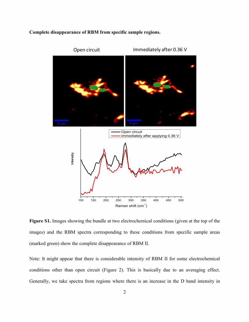
Complete disappearance of RBM from specific sample regions.

Open circuit Immediately after 0.36 V

100 150 200 250 300 350 400 450 500

Intensity

Raman shift (cm-1)

Open circuit

immediately after applying 0.36 V

Figure S1. Images showing the bundle at two electrochemical conditions (given at the top of the

images) and the RBM spectra corresponding to these conditions from specific sample areas

(marked green) show the complete disappearance of RBM II.

Note: It might appear that there is considerable intensity of RBM II for some electrochemical

conditions other than open circuit (Figure 2). This is basically due to an averaging effect.

Generally, we take spectra from regions where there is an increase in the D band intensity in

3

order to study the spectral evolution, as presented in Figure 2. It should be noted that the

unzipping process need not happen throughout the sample region under study due to the possible

inhomogeneity in the local potential. In order to clarify the statement that there is disappearance

of RBM II at 0.36 V, we have selected certain specific regions of the sample (marked by green

color in the above images) for two electrochemical conditions and averaged spectra from those

regions are presented above. It is evident that there is clear disappearance of RBMII.

4

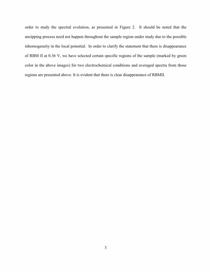
Variations of the spectral images at the intermittent electrode potentials.

RBM I RBM II RBM III

Figure S2. Evolution of RBM for various intermediate reduction steps corresponding to the

oxidizing steps given in Figure 2 of the main article. The types of RBMs are being labeled at the

top of each column. Each row gives the images of three RBMs at the conditions given at the left

of the respective row.

5

immediately after the

application of 0.36 V after 7 h of 0.36 V after 7 h of -0.36 V

after 7 h of -1.16 Vafter 7 h of 1.16 V after 7 h of 1.66 V

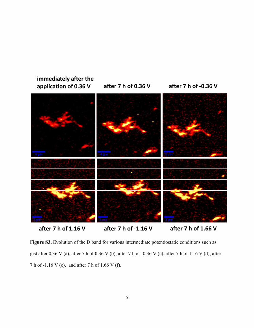
Figure S3. Evolution of the D band for various intermediate potentiostatic conditions such as

just after 0.36 V (a), after 7 h of 0.36 V (b), after 7 h of -0.36 V (c), after 7 h of 1.16 V (d), after

7 h of -1.16 V (e), and after 7 h of 1.66 V (f).

(f) (e) (d)

6

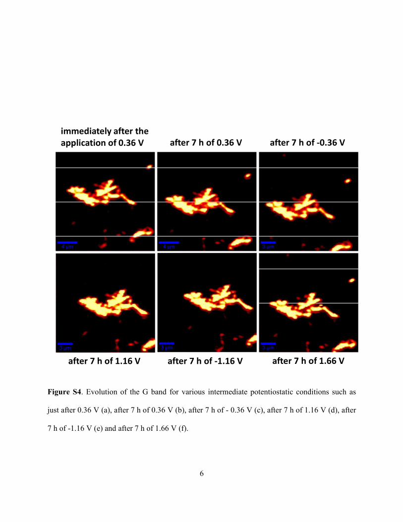
Figure S4. Evolution of the G band for various intermediate potentiostatic conditions such as

just after 0.36 V (a), after 7 h of 0.36 V (b), after 7 h of - 0.36 V (c), after 7 h of 1.16 V (d), after

7 h of -1.16 V (e) and after 7 h of 1.66 V (f).

immediately after the

application of 0.36 V after 7 h of 0.36 V after 7 h of -0.36 V

after 7 h of -1.16 Vafter 7 h of 1.16 V after 7 h of 1.66 V

7

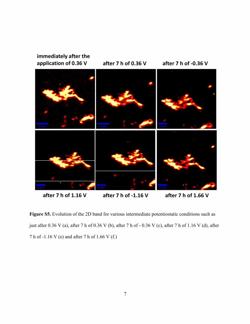
Figure S5. Evolution of the 2D band for various intermediate potentiostatic conditions such as

just after 0.36 V (a), after 7 h of 0.36 V (b), after 7 h of - 0.36 V (c), after 7 h of 1.16 V (d), after

7 h of -1.16 V (e) and after 7 h of 1.66 V (f.)

immediately after the

application of 0.36 V after 7 h of 0.36 V after 7 h of -0.36 V

after 7 h of -1.16 Vafter 7 h of 1.16 V after 7 h of 1.66 V

(d) (e) (f)

8

Reproducibility of Raman spectroscopic observations.

500 1000 1500 2000 2500

Inst

en

sity

Raman shift (cm-1)

0 V

just after 0.36 V

0.36 V for 7 h

-0.36 V for 7 h

1.16 V for 7 h

-1.16 V for 7 h

1.66 V for 7 h

-1.66 V for 7 h

150 200 250 300 350

Raman shift (cm-1)

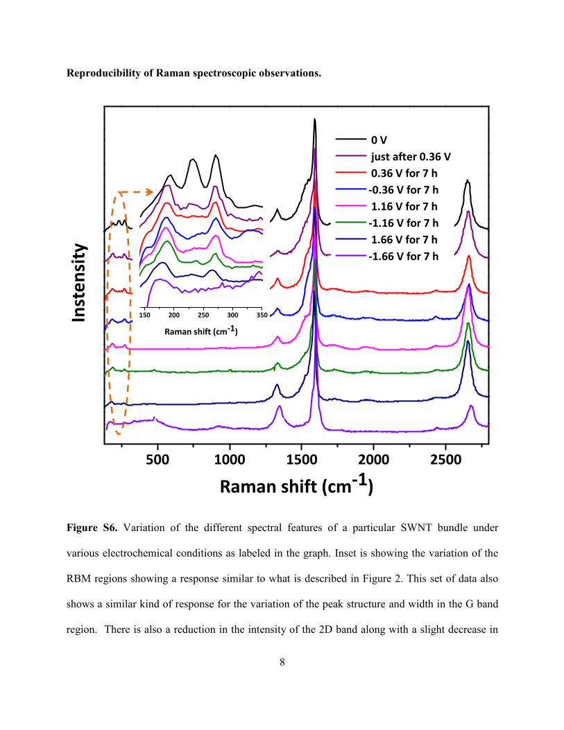
Figure S6. Variation of the different spectral features of a particular SWNT bundle under

various electrochemical conditions as labeled in the graph. Inset is showing the variation of the

RBM regions showing a response similar to what is described in Figure 2. This set of data also

shows a similar kind of response for the variation of the peak structure and width in the G band

region. There is also a reduction in the intensity of the 2D band along with a slight decrease in

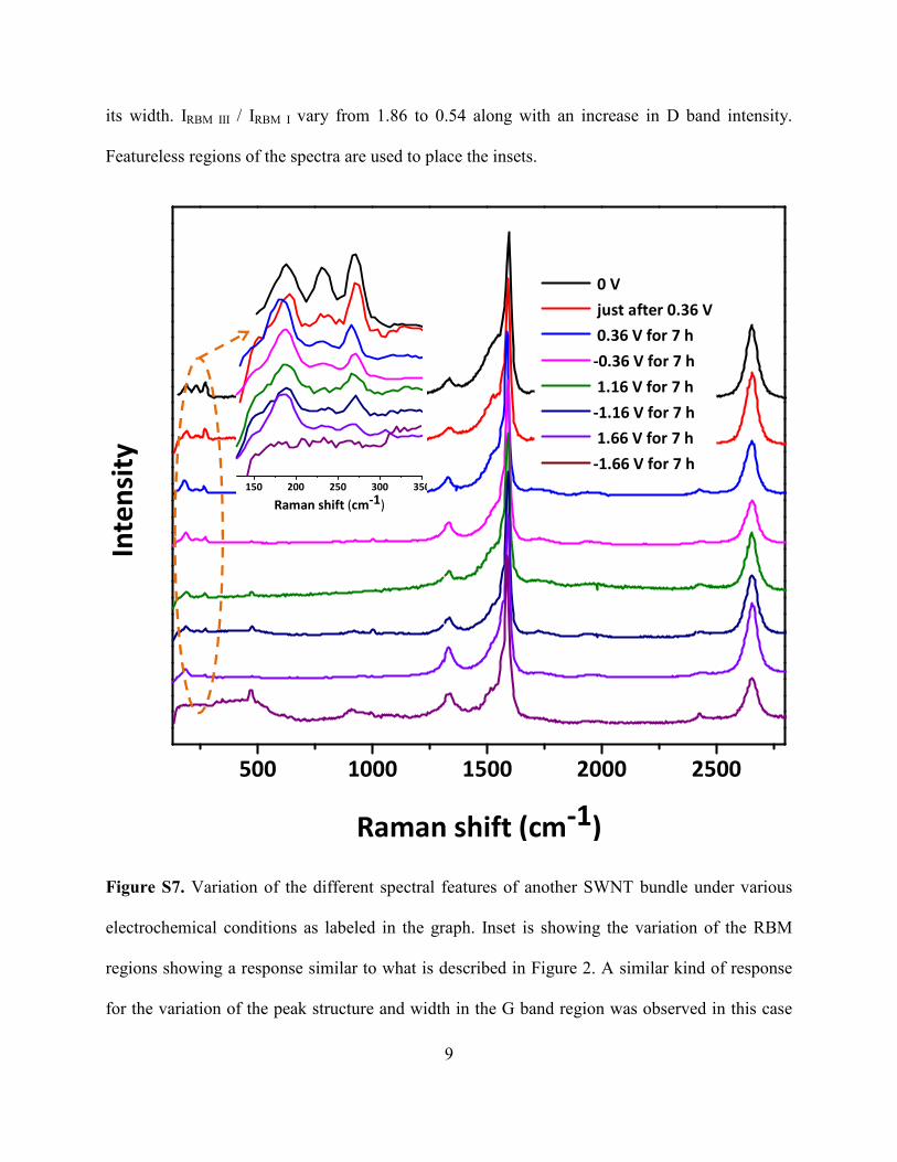
9

its width. IRBM III / IRBM I vary from 1.86 to 0.54 along with an increase in D band intensity.

Featureless regions of the spectra are used to place the insets.

500 1000 1500 2000 2500

Inte

nsi

ty

Raman shift (cm-1)

0 V

just after 0.36 V

0.36 V for 7 h

-0.36 V for 7 h

1.16 V for 7 h

-1.16 V for 7 h

1.66 V for 7 h

-1.66 V for 7 h

150 200 250 300 350

Raman shift (cm-1)

Figure S7. Variation of the different spectral features of another SWNT bundle under various

electrochemical conditions as labeled in the graph. Inset is showing the variation of the RBM

regions showing a response similar to what is described in Figure 2. A similar kind of response

for the variation of the peak structure and width in the G band region was observed in this case

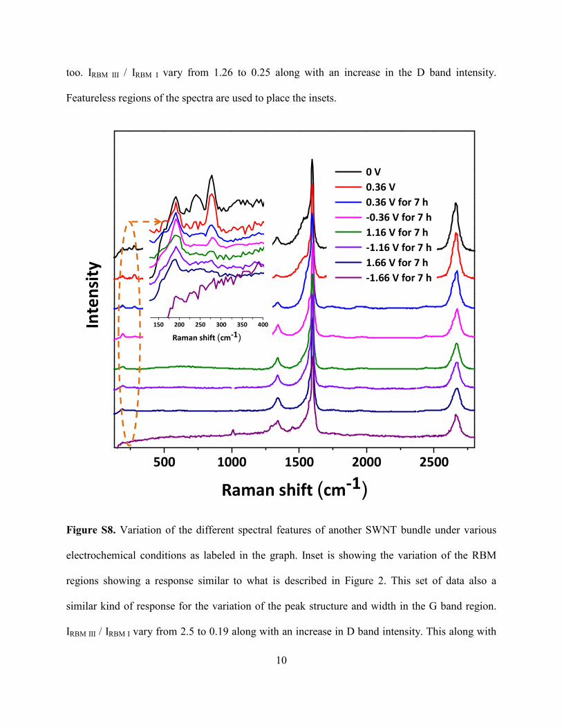
10

too. IRBM III / IRBM I vary from 1.26 to 0.25 along with an increase in the D band intensity.

Featureless regions of the spectra are used to place the insets.

500 1000 1500 2000 2500

Inte

nsi

ty

Raman shift (cm-1)

0 V

0.36 V

0.36 V for 7 h

-0.36 V for 7 h

1.16 V for 7 h

-1.16 V for 7 h

1.66 V for 7 h

-1.66 V for 7 h

150 200 250 300 350 400

Raman shift (cm-1)

Figure S8. Variation of the different spectral features of another SWNT bundle under various

electrochemical conditions as labeled in the graph. Inset is showing the variation of the RBM

regions showing a response similar to what is described in Figure 2. This set of data also a

similar kind of response for the variation of the peak structure and width in the G band region.

IRBM III / IRBM I vary from 2.5 to 0.19 along with an increase in D band intensity. This along with

11

Figure S6 and S7 shows the reproducibility of the experimental results presented in the

manuscript. Featureless regions of the spectra are used to place the insets.

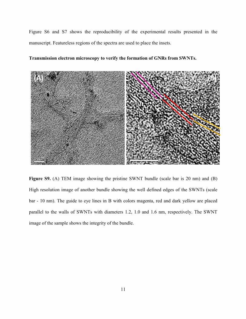
Transmission electron microscopy to verify the formation of GNRs from SWNTs.

(A) (B)

10 nm

Figure S9. (A) TEM image showing the pristine SWNT bundle (scale bar is 20 nm) and (B)

High resolution image of another bundle showing the well defined edges of the SWNTs (scale

bar - 10 nm). The guide to eye lines in B with colors magenta, red and dark yellow are placed

parallel to the walls of SWNTs with diameters 1.2, 1.0 and 1.6 nm, respectively. The SWNT

image of the sample shows the integrity of the bundle.

12

(A) (B)

(D)(C)

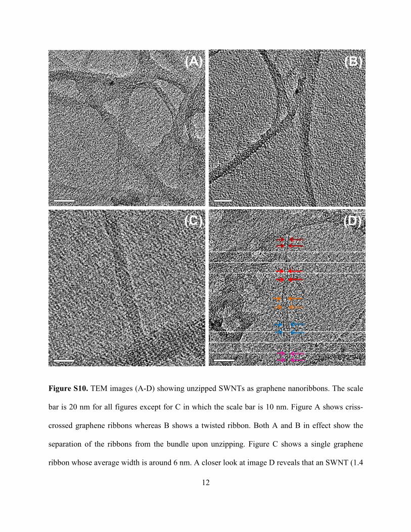
Figure S10. TEM images (A-D) showing unzipped SWNTs as graphene nanoribbons. The scale

bar is 20 nm for all figures except for C in which the scale bar is 10 nm. Figure A shows criss-

crossed graphene ribbons whereas B shows a twisted ribbon. Both A and B in effect show the

separation of the ribbons from the bundle upon unzipping. Figure C shows a single graphene

ribbon whose average width is around 6 nm. A closer look at image D reveals that an SWNT (1.4

13

nm, wine red colored arrows) opens up into a graphene ribbon (5 nm, blue colored arrows). The

width is 2.5 nm where the red arrows are present and it is 4 nm where the dark yellow arrows are

pointed at. The bottom part of the image shows a narrow ribbon of width 3.5 nm (magenta

arrows). Considering the diameters of the SWNTs used, this image represent most likely the

partial unzipping of an SWNT and it appears that the unzipping originates at the middle portion

(lengthwise) of the side wall rather than at the ends of the nanotubes.

Evolution of the G Band region to show the reduction in metallicity.

1200 1600 2000 2400 2800

0.2

0.4

0.6

0.8

1.0

1.2

2D

D

G*

Inte

nsi

ty (

arb

itra

y u

nit

)

Raman shift (cm-1)

experimental spectrum

D band

G* band

G band

2D band

Sum of the peaks

G

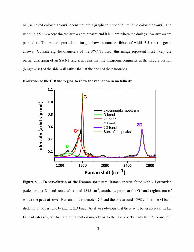
Figure S11. Deconvolution of the Raman spectrum. Raman spectra fitted with 4 Lorentzian

peaks, one at D band centered around 1345 cm-1, another 2 peaks at the G band region, out of

which the peak at lower Raman shift is denoted G* and the one around 1598 cm-1 is the G band

itself with the last one being the 2D band. As it was obvious that there will be an increase in the

D band intensity, we focused our attention majorly on to the last 3 peaks namely, G*, G and 2D.

14

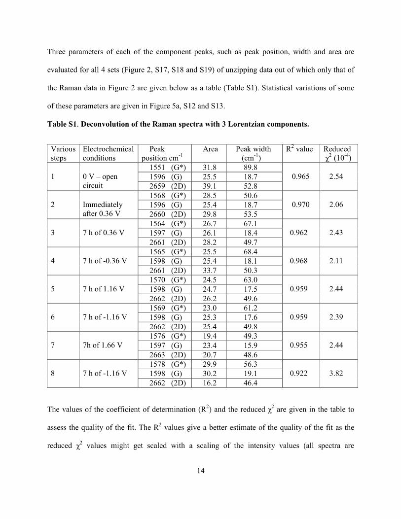
Three parameters of each of the component peaks, such as peak position, width and area are

evaluated for all 4 sets (Figure 2, S17, S18 and S19) of unzipping data out of which only that of

the Raman data in Figure 2 are given below as a table (Table S1). Statistical variations of some

of these parameters are given in Figure 5a, S12 and S13.

Table S1. Deconvolution of the Raman spectra with 3 Lorentzian components.

Various steps

Electrochemical conditions

Peak position cm-1

Area Peak width (cm-1)

R2 value Reduced χ2 (10-4)

1

0 V – open circuit

1551 (G*) 31.8 89.8 0.965

2.54 1596 (G) 25.5 18.7

2659 (2D) 39.1 52.8 2

Immediately after 0.36 V

1568 (G*) 28.5 50.6 0.970

2.06 1596 (G) 25.4 18.7

2660 (2D) 29.8 53.5 3

7 h of 0.36 V

1564 (G*) 26.7 67.1 0.962

2.43 1597 (G) 26.1 18.4

2661 (2D) 28.2 49.7 4

7 h of -0.36 V

1565 (G*) 25.5 68.4 0.968

2.11 1598 (G) 25.4 18.1

2661 (2D) 33.7 50.3 5

7 h of 1.16 V

1570 (G*) 24.5 63.0 0.959

2.44 1598 (G) 24.7 17.5

2662 (2D) 26.2 49.6 6

7 h of -1.16 V

1569 (G*) 23.0 61.2 0.959

2.39 1598 (G) 25.3 17.6

2662 (2D) 25.4 49.8 7

7h of 1.66 V

1576 (G*) 19.4 49.3 0.955

2.44 1597 (G) 23.4 15.9

2663 (2D) 20.7 48.6 8

7 h of -1.16 V

1578 (G*) 29.9 56.3 0.922

3.82 1598 (G) 30.2 19.1

2662 (2D) 16.2 46.4

The values of the coefficient of determination (R2) and the reduced χ2 are given in the table to

assess the quality of the fit. The R2 values give a better estimate of the quality of the fit as the

reduced χ2 values might get scaled with a scaling of the intensity values (all spectra are

15

normalized using the G band and translated vertically for clarity). The peak widths given in the

table are full width at half maximum (FWHM). The possibility of giving a similar deconvolution

data for the RBM region will be improper as the intensity of RBM peaks are generally very less

and also because of the lack of proper peak shape owing to the low intensity. Also there can be a

confusion arising due to the averaging effect as discussed in Figure S1 and the following text.

0 1 2 3 4 5 6 7 8 9

20

40

60

80

100

120

140

Pe

ak

wid

th o

f G

* b

an

d

Various steps

0 1 2 3 4 5 6 7 8 9

1535

1540

1545

1550

1555

1560

1565

1570

1575

Pe

ak

po

siti

on

of

G*

ba

nd

Various steps

(a) (b)

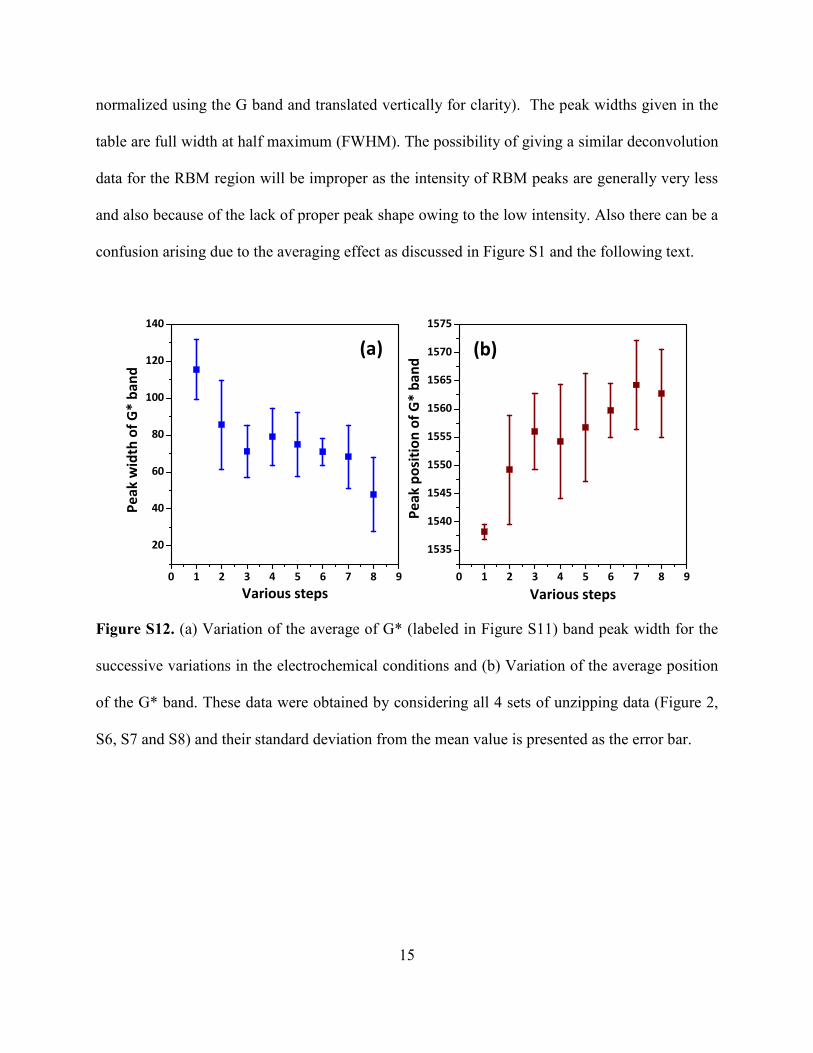
Figure S12. (a) Variation of the average of G* (labeled in Figure S11) band peak width for the

successive variations in the electrochemical conditions and (b) Variation of the average position

of the G* band. These data were obtained by considering all 4 sets of unzipping data (Figure 2,

S6, S7 and S8) and their standard deviation from the mean value is presented as the error bar.

16

1 2 3 4 5 6 7 8

42

44

46

48

50

52

54

56

58

60

2D

ba

nd

wid

th

Various steps

Figure S13. Variation of the width of the Lorentian peak fitted to the 2D band centered at 2660

cm-1. This data was obtained by considering all 4 sets of unzipping data (Figure 2, S6, S7 and

S8) and their standard deviation from the mean value is presented as the error bar.

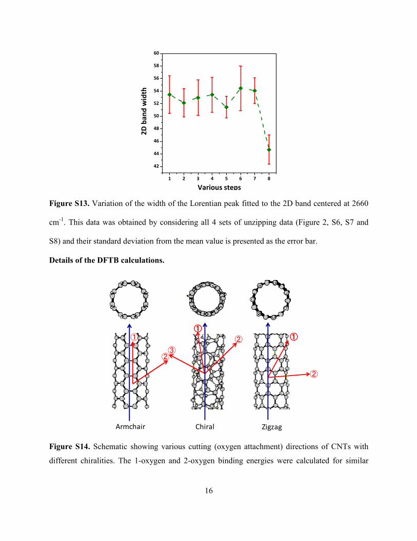
Details of the DFTB calculations.

Armchair

➁

Chiral

➀➀➀➀

➁

➂

Zigzag

➀➀➀➀

➁

➀

Figure S14. Schematic showing various cutting (oxygen attachment) directions of CNTs with

different chiralities. The 1-oxygen and 2-oxygen binding energies were calculated for similar

17

directions of the SWNTs having chiral indices of interest and presented in the following

discussion.

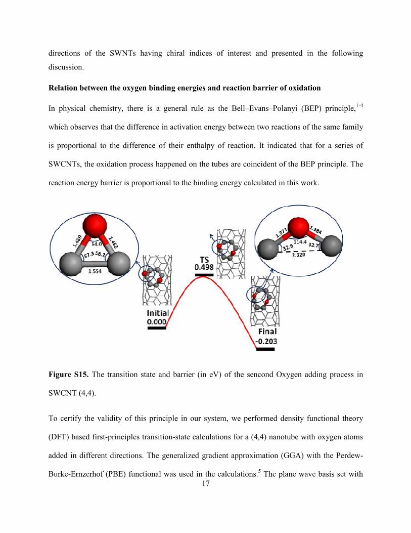
Relation between the oxygen binding energies and reaction barrier of oxidation

In physical chemistry, there is a general rule as the Bell–Evans–Polanyi (BEP) principle,1-4

which observes that the difference in activation energy between two reactions of the same family

is proportional to the difference of their enthalpy of reaction. It indicated that for a series of

SWCNTs, the oxidation process happened on the tubes are coincident of the BEP principle. The

reaction energy barrier is proportional to the binding energy calculated in this work.

Figure S15. The transition state and barrier (in eV) of the sencond Oxygen adding process in

SWCNT (4,4).

To certify the validity of this principle in our system, we performed density functional theory

(DFT) based first-principles transition-state calculations for a (4,4) nanotube with oxygen atoms

added in different directions. The generalized gradient approximation (GGA) with the Perdew-

Burke-Ernzerhof (PBE) functional was used in the calculations.5 The plane wave basis set with

18

an energy cutoff of 400 eV was used and the criterion of convergence is set as the force on atom

below 0.03 eV/Å. The transition states were searched and their barriers were calculated by the

climbing nudged energy band (cNEB) method as implemented in the Vienna Ab initio Software

Package (VASP).6,7 It is found that if the oxygen adding direction (defined by the angle θ along

the tube axis) of (4,4) nanotube is 0o, the transition state does not exist, indicating a spontaneous

reaction. However, if θ = 60o, there is an energy barrier of 0.498 eV (see Figure S15). It turns out

that SWNTs with smaller diameters have higher oxygen binding energies and binding oxygen

atoms through epoxy groups is preferred. The transition states calculations are consistent with

the BEP principle, allowing us to make the abovementioned conclusion with DFTB calculations

for the oxygen binding energies.

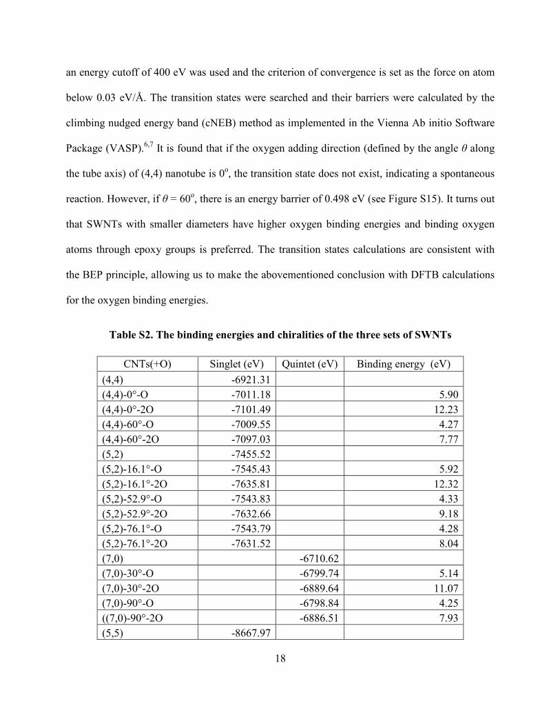
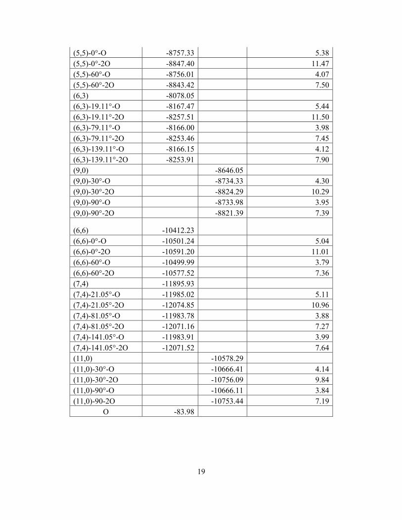
Table S2. The binding energies and chiralities of the three sets of SWNTs

CNTs(+O) Singlet (eV) Quintet (eV) Binding energy (eV)

(4,4) -6921.31

(4,4)-0°-O -7011.18 5.90

(4,4)-0°-2O -7101.49 12.23

(4,4)-60°-O -7009.55 4.27

(4,4)-60°-2O -7097.03 7.77

(5,2) -7455.52

(5,2)-16.1°-O -7545.43 5.92

(5,2)-16.1°-2O -7635.81 12.32

(5,2)-52.9°-O -7543.83 4.33

(5,2)-52.9°-2O -7632.66 9.18

(5,2)-76.1°-O -7543.79 4.28

(5,2)-76.1°-2O -7631.52 8.04

(7,0) -6710.62

(7,0)-30°-O -6799.74 5.14

(7,0)-30°-2O -6889.64 11.07

(7,0)-90°-O -6798.84 4.25

((7,0)-90°-2O -6886.51 7.93

(5,5) -8667.97

19

(5,5)-0°-O -8757.33 5.38

(5,5)-0°-2O -8847.40 11.47

(5,5)-60°-O -8756.01 4.07

(5,5)-60°-2O -8843.42 7.50

(6,3) -8078.05

(6,3)-19.11°-O -8167.47 5.44

(6,3)-19.11°-2O -8257.51 11.50

(6,3)-79.11°-O -8166.00 3.98

(6,3)-79.11°-2O -8253.46 7.45

(6,3)-139.11°-O -8166.15 4.12

(6,3)-139.11°-2O -8253.91 7.90

(9,0) -8646.05

(9,0)-30°-O -8734.33 4.30

(9,0)-30°-2O -8824.29 10.29

(9,0)-90°-O -8733.98 3.95

(9,0)-90°-2O -8821.39 7.39

(6,6) -10412.23

(6,6)-0°-O -10501.24 5.04

(6,6)-0°-2O -10591.20 11.01

(6,6)-60°-O -10499.99 3.79

(6,6)-60°-2O -10577.52 7.36

(7,4) -11895.93

(7,4)-21.05°-O -11985.02 5.11

(7,4)-21.05°-2O -12074.85 10.96

(7,4)-81.05°-O -11983.78 3.88

(7,4)-81.05°-2O -12071.16 7.27

(7,4)-141.05°-O -11983.91 3.99

(7,4)-141.05°-2O -12071.52 7.64

(11,0) -10578.29

(11,0)-30°-O -10666.41 4.14

(11,0)-30°-2O -10756.09 9.84

(11,0)-90°-O -10666.11 3.84

(11,0)-90-2O -10753.44 7.19

O -83.98

20

Figure S16. The relationship between the binding energy (Eb) of the CNTs + nO (n = 1, 2) and

and the nO addition angle with respect to the tube axis of SWNTs in the first set of calculations.

Details are given in Table S2.

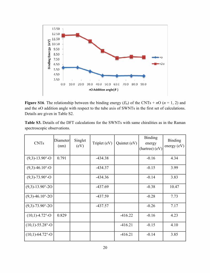
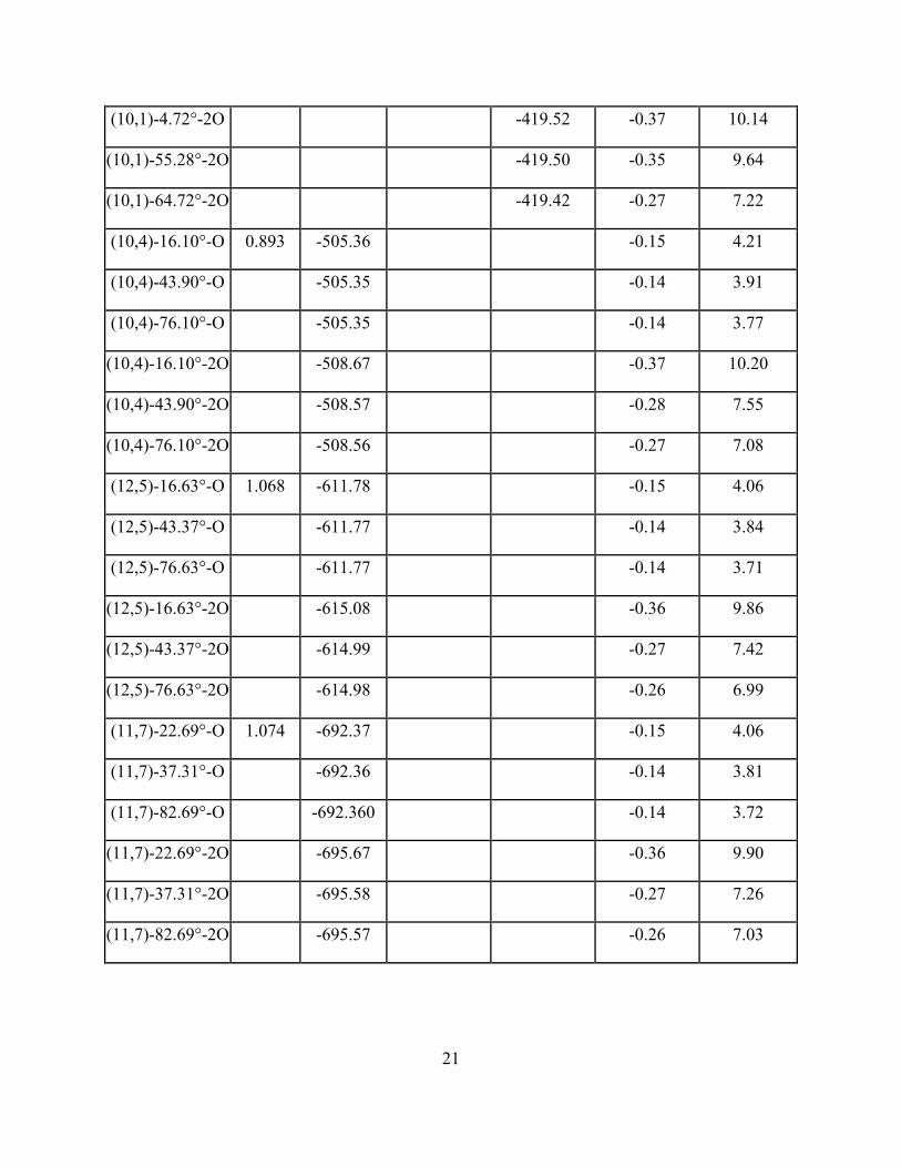
Table S3. Details of the DFT calculations for the SWNTs with same chiralities as in the Raman

spectroscopic observations.

CNTs Diameter

(nm)

Singlet

(eV) Triplet (eV) Quintet (eV)

Binding

energy

(hartree) (eV)

Binding

energy (eV)

(9,3)-13.90°-O 0.791

-434.38

-0.16 4.34

(9,3)-46.10°-O

-434.37

-0.15 3.99

(9,3)-73.90°-O

-434.36

-0.14 3.83

(9,3)-13.90°-2O

-437.69

-0.38 10.47

(9,3)-46.10°-2O

-437.59

-0.28 7.73

(9,3)-73.90°-2O

-437.57

-0.26 7.17

(10,1)-4.72°-O 0.829

-416.22 -0.16 4.23

(10,1)-55.28°-O

-416.21 -0.15 4.10

(10,1)-64.72°-O

-416.21 -0.14 3.85

21

(10,1)-4.72°-2O

-419.52 -0.37 10.14

(10,1)-55.28°-2O

-419.50 -0.35 9.64

(10,1)-64.72°-2O

-419.42 -0.27 7.22

(10,4)-16.10°-O 0.893 -505.36

-0.15 4.21

(10,4)-43.90°-O

-505.35

-0.14 3.91

(10,4)-76.10°-O

-505.35

-0.14 3.77

(10,4)-16.10°-2O

-508.67

-0.37 10.20

(10,4)-43.90°-2O

-508.57

-0.28 7.55

(10,4)-76.10°-2O

-508.56

-0.27 7.08

(12,5)-16.63°-O 1.068 -611.78

-0.15 4.06

(12,5)-43.37°-O

-611.77

-0.14 3.84

(12,5)-76.63°-O

-611.77

-0.14 3.71

(12,5)-16.63°-2O

-615.08

-0.36 9.86

(12,5)-43.37°-2O

-614.99

-0.27 7.42

(12,5)-76.63°-2O

-614.98

-0.26 6.99

(11,7)-22.69°-O 1.074 -692.37

-0.15 4.06

(11,7)-37.31°-O

-692.36

-0.14 3.81

(11,7)-82.69°-O

-692.360

-0.14 3.72

(11,7)-22.69°-2O

-695.67

-0.36 9.90

(11,7)-37.31°-2O

-695.58

-0.27 7.26

(11,7)-82.69°-2O

-695.57

-0.26 7.03

22

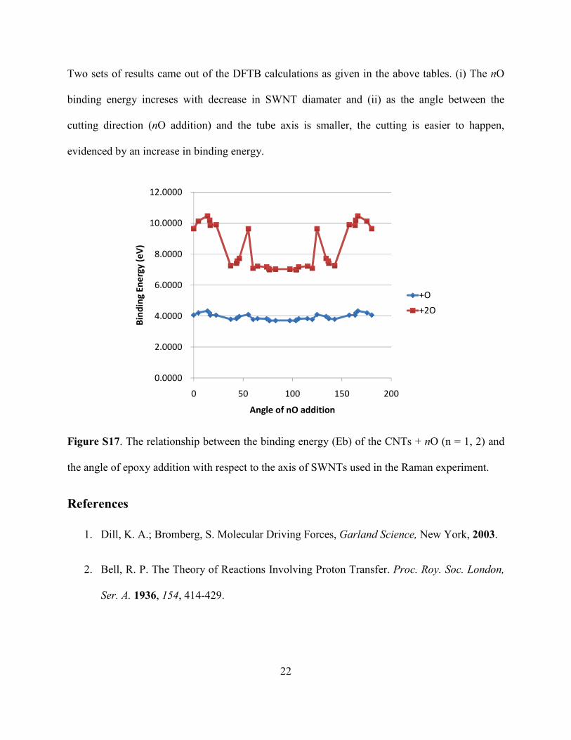
Two sets of results came out of the DFTB calculations as given in the above tables. (i) The nO

binding energy increses with decrease in SWNT diamater and (ii) as the angle between the

cutting direction (nO addition) and the tube axis is smaller, the cutting is easier to happen,

evidenced by an increase in binding energy.

0.0000

2.0000

4.0000

6.0000

8.0000

10.0000

12.0000

0 50 100 150 200

Bin

din

g E

ne

rgy

(e

V)

Angle of nO addition

+O

+2O

Figure S17. The relationship between the binding energy (Eb) of the CNTs + nO (n = 1, 2) and

the angle of epoxy addition with respect to the axis of SWNTs used in the Raman experiment.

References

1. Dill, K. A.; Bromberg, S. Molecular Driving Forces, Garland Science, New York, 2003.

2. Bell, R. P. The Theory of Reactions Involving Proton Transfer. Proc. Roy. Soc. London,

Ser. A. 1936, 154, 414-429.

23

3. Evans, M. G.; Polanyi, M. Some Applications of the Transition State Method to the

Calculation of Reaction Velocities, Especially in Solution. Trans. Faraday Soc. 1935, 31,

875-894.

4. Evans, M. G.; Polanyi, M. Inertia and Driving Force of Chemical Reactions. Trans.

Faraday Soc. 1938, 34, 11-24.

5. Perdew, J. P.; Burke, K.; Ernzerhof, M. Generalized Gradient Approximation Made

Simple. Phys. Rev. Lett. 1996, 77, 3865-3868.

6. Kresse, G.; Furthmuller, J. Efficient Iterative Schemes for ab-initio Total Energy

Calculations Using a Plane-Wave Basis Set. Phys. Rev. B 1996, 54, 11169-11186.

7. Kresse, G.; Furthmuller, J. Efficiency of ab-initio Total Energy Calculations for Metals

and Semiconductors Using a Plane-Wave Basis Set. Comput. Mater. Sci. 1996, 6, 15-50.