1 Random Variable A random variable X is a function that assign a real number, X(ζ), to each...
32
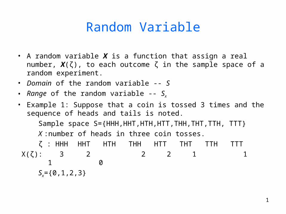
1 Random Variable • A random variable X is a function that assign a real number, X(ζ), to each outcome ζ in the sample space of a random experiment. • Domain of the random variable -- S • Range of the random variable -- S x • Example 1: Suppose that a coin is tossed 3 times and the sequence of heads and tails is noted. Sample space S={HHH,HHT,HTH,HTT,THH,THT,TTH, TTT} X :number of heads in three coin tosses. ζ : HHH HHT HTH THH HTT THT TTH TTT X(ζ): 3 2 2 2 1 1 1 0 S x ={0,1,2,3}
-
Upload
linda-long -
Category
Documents
-
view
235 -
download
0
Transcript of 1 Random Variable A random variable X is a function that assign a real number, X(ζ), to each...
1
Random Variable
• A random variable X is a function that assign a real number, X(ζ), to each outcome ζ in the sample space of a random experiment.
• Domain of the random variable -- S
• Range of the random variable -- Sx
• Example 1: Suppose that a coin is tossed 3 times and the sequence of heads and tails is noted.
Sample space S={HHH,HHT,HTH,HTT,THH,THT,TTH, TTT}
X :number of heads in three coin tosses.
ζ : HHHHHT HTH THH HTT THT TTH TTT
X(ζ): 3 2 2 2 1 1 1 0
Sx={0,1,2,3}
2
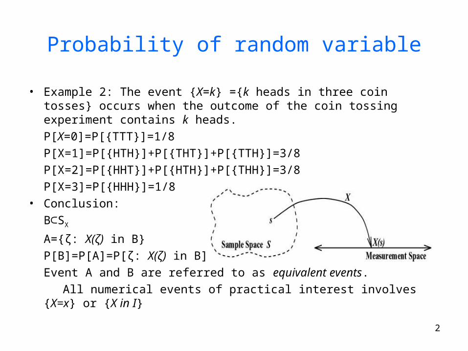
Probability of random variable
• Example 2: The event {X=k} ={k heads in three coin tosses} occurs when the outcome of the coin tossing experiment contains k heads.
P[X=0]=P[{TTT}]=1/8
P[X=1]=P[{HTH}]+P[{THT}]+P[{TTH}]=3/8
P[X=2]=P[{HHT}]+P[{HTH}]+P[{THH}]=3/8
P[X=3]=P[{HHH}]=1/8• Conclusion:
B⊂SX
A={ζ: X(ζ) in B}
P[B]=P[A]=P[ζ: X(ζ) in B].
Event A and B are referred to as equivalent events.
All numerical events of practical interest involves {X=x} or {X in I}
3
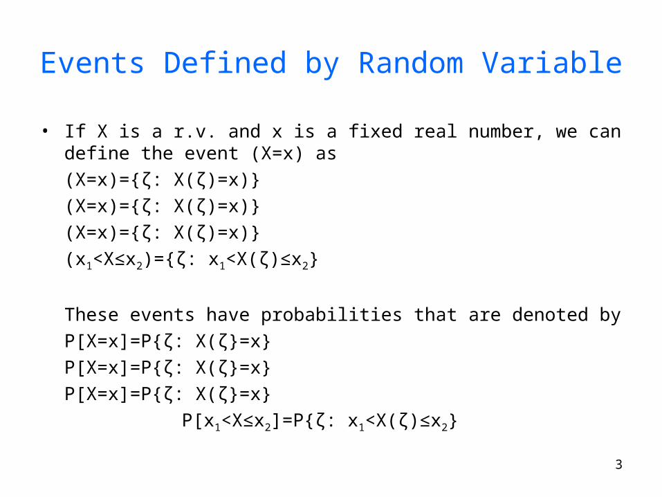
Events Defined by Random Variable
• If X is a r.v. and x is a fixed real number, we can define the event (X=x) as
(X=x)={ζ: X(ζ)=x)}
(X=x)={ζ: X(ζ)=x)}
(X=x)={ζ: X(ζ)=x)}
(x1<X≤x2)={ζ: x1<X(ζ)≤x2}
These events have probabilities that are denoted by
P[X=x]=P{ζ: X(ζ}=x}
P[X=x]=P{ζ: X(ζ}=x}
P[X=x]=P{ζ: X(ζ}=x}
P[x1<X≤x2]=P{ζ: x1<X(ζ)≤x2}
4
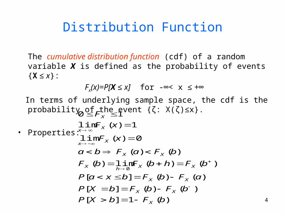
Distribution Function
The cumulative distribution function (cdf) of a random variable X is defined as the probability of events {X ≤ x}:
Fx(x)=P[X ≤ x] for -∞< x ≤ +∞
In terms of underlying sample space, the cdf is the probability of the event {ζ: X(ζ)≤x}.
• Properties:
)(1][
)()(][
)()(][
)()(lim)(
)()(
0)(lim
1)(lim
10
0
bFbXP
bFbFbXP
aFbFbxaP
bFhbFbF
bFaFba
xF
xF
F
X
XX
XX
XXh
X
XX
Xx
Xx
X
5
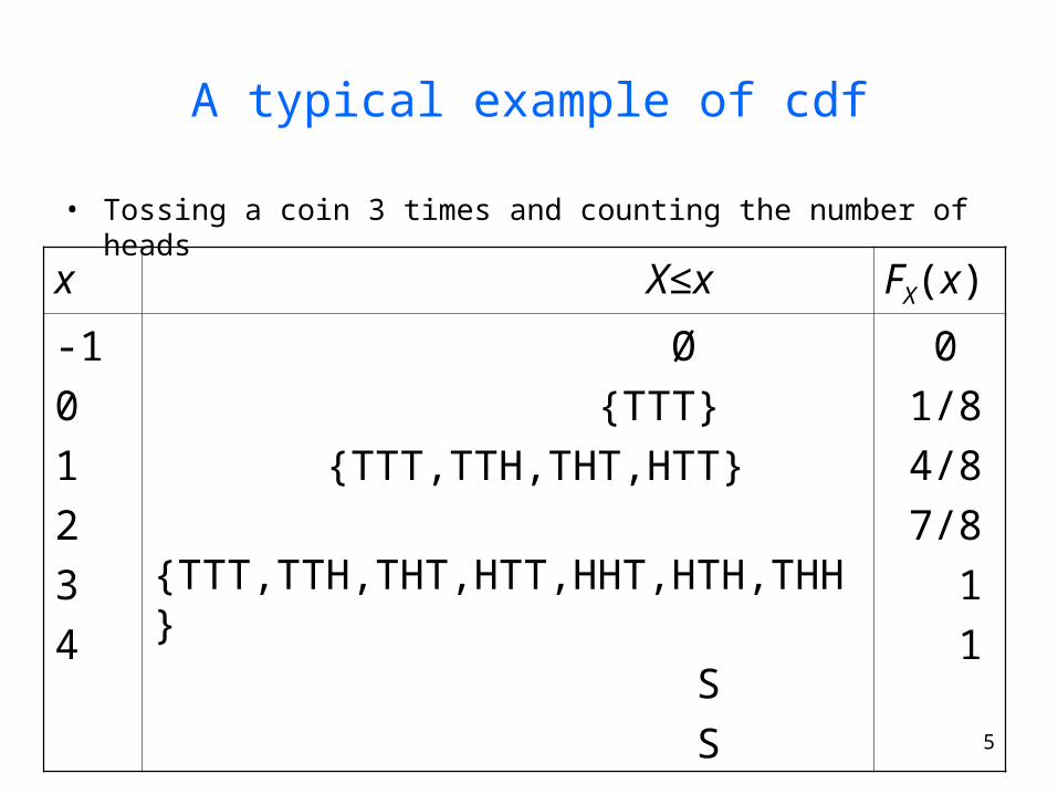
A typical example of cdf
• Tossing a coin 3 times and counting the number of heads
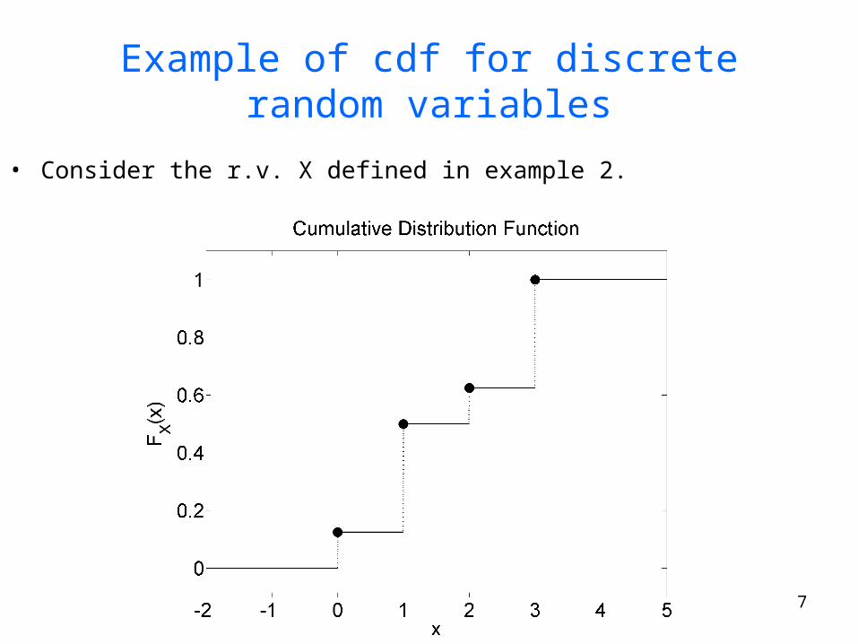
x X≤x FX(x)
-1
0
1
2
3
4
Ø
{TTT}
{TTT,TTH,THT,HTT}
{TTT,TTH,THT,HTT,HHT,HTH,THH}
S
S
0
1/8
4/8
7/8
1
1
6
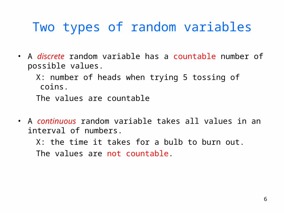
Two types of random variables
• A discrete random variable has a countable number of possible values.
X: number of heads when trying 5 tossing of coins.
The values are countable
• A continuous random variable takes all values in an interval of numbers.
X: the time it takes for a bulb to burn out.
The values are not countable.
7
Example of cdf for discrete random variables
• Consider the r.v. X defined in example 2.
8
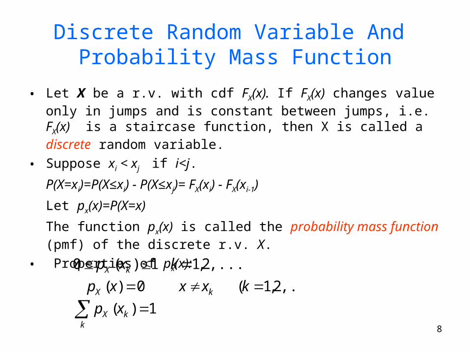
Discrete Random Variable And Probability Mass Function
• Let X be a r.v. with cdf FX(x). If FX(x) changes value only in jumps and is constant between jumps, i.e. FX(x) is a staircase function, then X is called a discrete random variable.
• Suppose xi < xj if i<j.
P(X=xi)=P(X≤xi) - P(X≤xj)= FX(xi) - FX(xi-1)
Let px(x)=P(X=x)
The function px(x) is called the probability mass function (pmf) of the discrete r.v. X.
• Properties of px(x):
kkX
kX
kX
xp
kxxxp
kxp
1)(
,...)2,1(0)(
,...2,11)(0
9
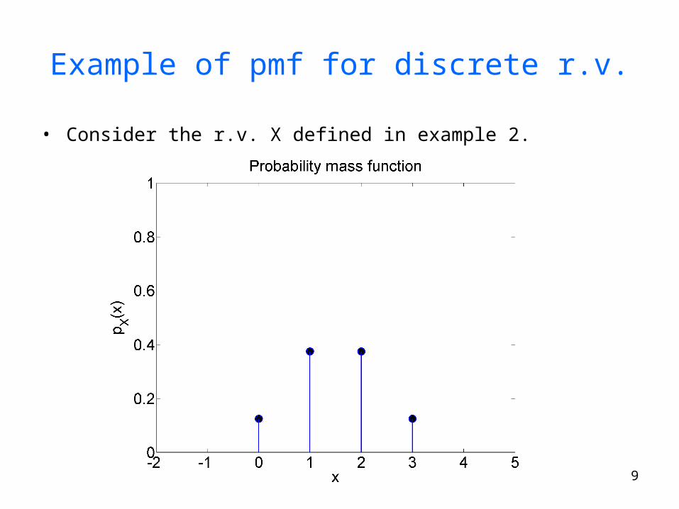
Example of pmf for discrete r.v.
• Consider the r.v. X defined in example 2.
10
Continuous Random variable and Probability Density function
• Let X be a r.v. with cdf FX(x) . If FX(x) is continuous and also has a derivative dFX(x) /dx which exist everywhere except at possibly a finite number of points and is piecewise continuous, then X is called a continuous random variable.
• Let
• The function fX(x) is called the probability density function (pdf) of the continuous r.v. X . fX(x) is piecewise continuous.
• Properties:
dx
xdFxf X
X
)()(
b
a X
X
X
dxxfbXaP
dxxf
xf
)()(
1)(
0)(
11
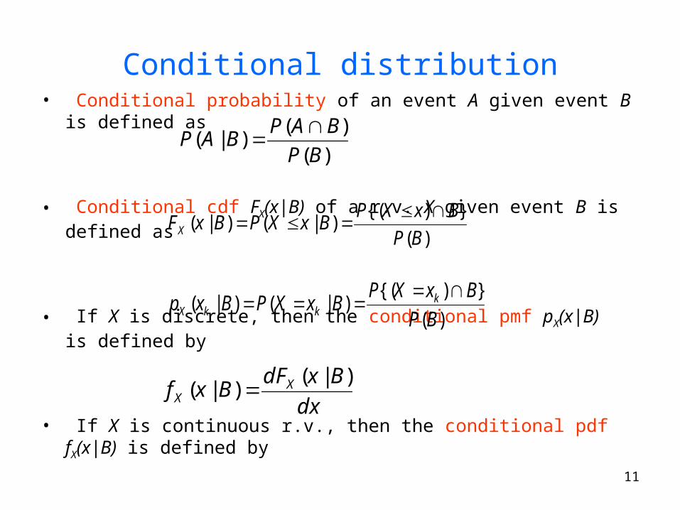
Conditional distribution• Conditional probability of an event A given event B is defined as
• Conditional cdf FX(x|B) of a r.v. X given event B is defined as
• If X is discrete, then the conditional pmf pX(x|B) is defined by
• If X is continuous r.v., then the conditional pdf fX(x|B) is defined by
)(
)()|(
BP
BAPBAP
)(
}){()|()|(
BP
BxXPBxXPBxFX
dx
BxdFBxf X
X
)|()|(
)(
}){()|()|(
BP
BxXPBxXPBxp k
kkX
12
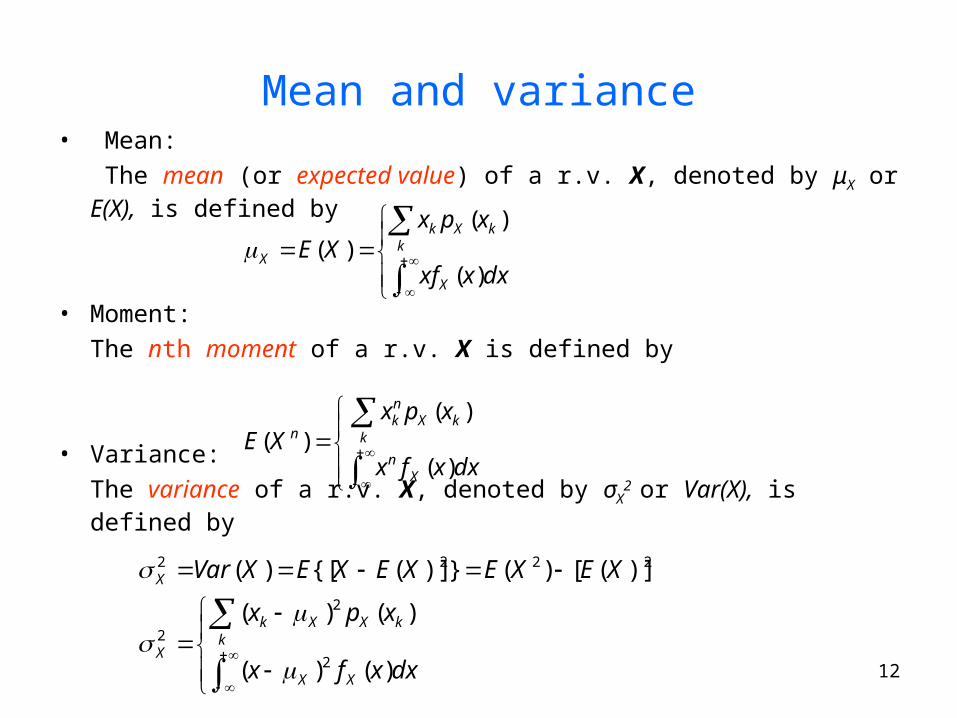
Mean and variance• Mean:
The mean (or expected value) of a r.v. X, denoted by μX or E(X), is defined by
• Moment:
The nth moment of a r.v. X is defined by
• Variance:
The variance of a r.v. X, denoted by σX2 or Var(X), is defined by
dxxxf
xpxXE
X
kkXk
X
)(
)()(
dxxfx
xpxXE
Xn
kkX
nk
n
)(
)()(
dxxfx
xpx
XEXEXEXEXVar
XX
kkXXk
X
X
)()(
)()(
)]([)(})]({[)(
2
2
2
2222

13
Expectation of a Function of a Random variable
• Given a r.v. X and its probability distribution (pmf in the discrete case and pdf in the continuous case), how to calculate the expected value of some function of X, E(g(X))?
• Proposition:
(a) If X is a discrete r.v. with pmf pX(x), then for any real-valued function g,
(b) If X is a continuous r.v. with pdf fX(x), then for any real-valued function g,
k
kk xpxgXgE )()()]([
dxxfxgXgE )()()]([
14
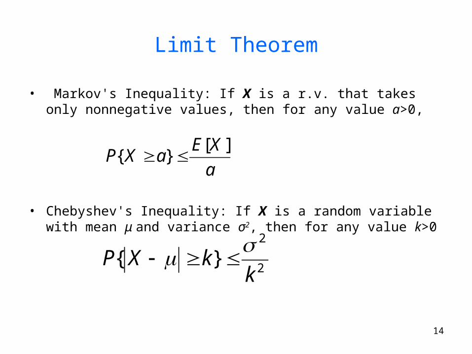
Limit Theorem
• Markov's Inequality: If X is a r.v. that takes only nonnegative values, then for any value a>0,
• Chebyshev's Inequality: If X is a random variable with mean μ and variance σ2, then for any value k>0
a
XEaXP
][}{
2
2
}{k
kXP
15
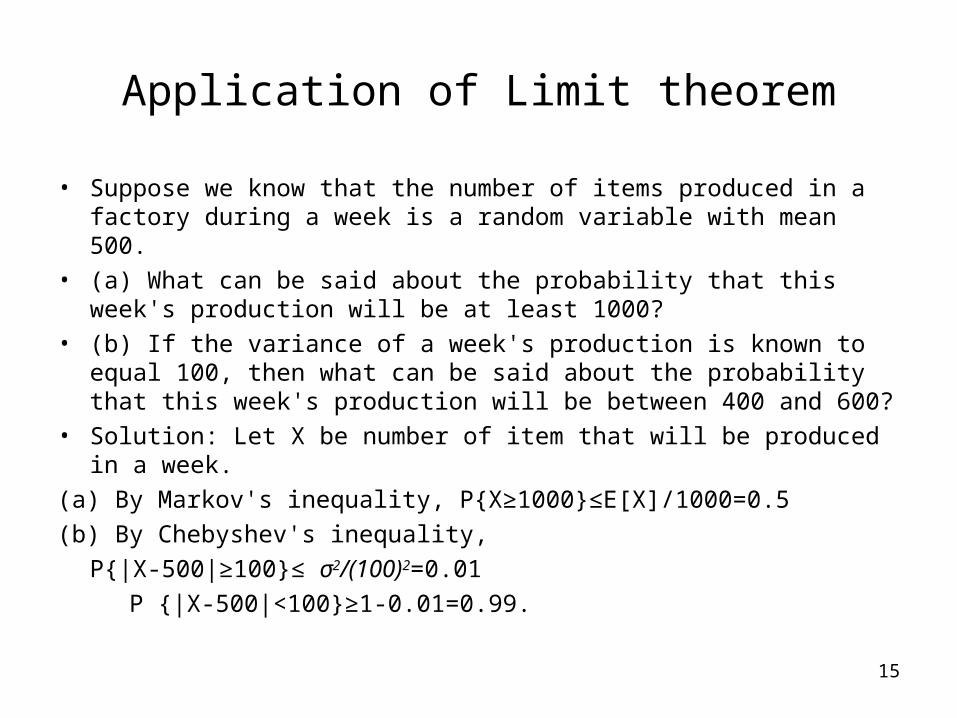
Application of Limit theorem
• Suppose we know that the number of items produced in a factory during a week is a random variable with mean 500.
• (a) What can be said about the probability that this week's production will be at least 1000?
• (b) If the variance of a week's production is known to equal 100, then what can be said about the probability that this week's production will be between 400 and 600?
• Solution: Let X be number of item that will be produced in a week.
(a) By Markov's inequality, P{X≥1000}≤E[X]/1000=0.5
(b) By Chebyshev's inequality,
P{|X-500|≥100}≤ σ2/(100)2=0.01
P {|X-500|<100}≥1-0.01=0.99.
16
Some Special Distribution
• Bernoulli Distribution• Binomial Distribution• Poisson Distribution• Uniform Distribution• Exponential Distribution• Normal (or Gaussian) Distribution• Conditional Distribution• ……
17
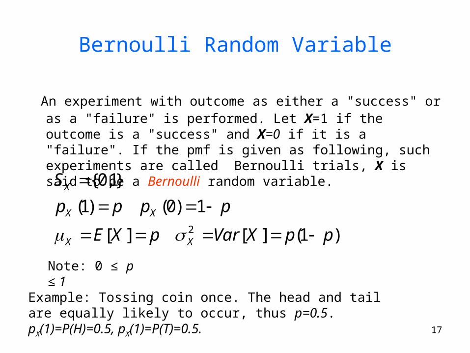
Bernoulli Random Variable
An experiment with outcome as either a "success" or as a "failure" is performed. Let X=1 if the outcome is a "success" and X=0 if it is a "failure". If the pmf is given as following, such experiments are called Bernoulli trials, X is said to be a Bernoulli random variable.
)1(][][
1)0()1(
}1,0{
2 ppXVarpXE
pppp
S
XX
XX
X
Note: 0 ≤ p ≤ 1
Example: Tossing coin once. The head and tail are equally likely to occur, thus p=0.5. pX(1)=P(H)=0.5, pX(1)=P(T)=0.5.
18
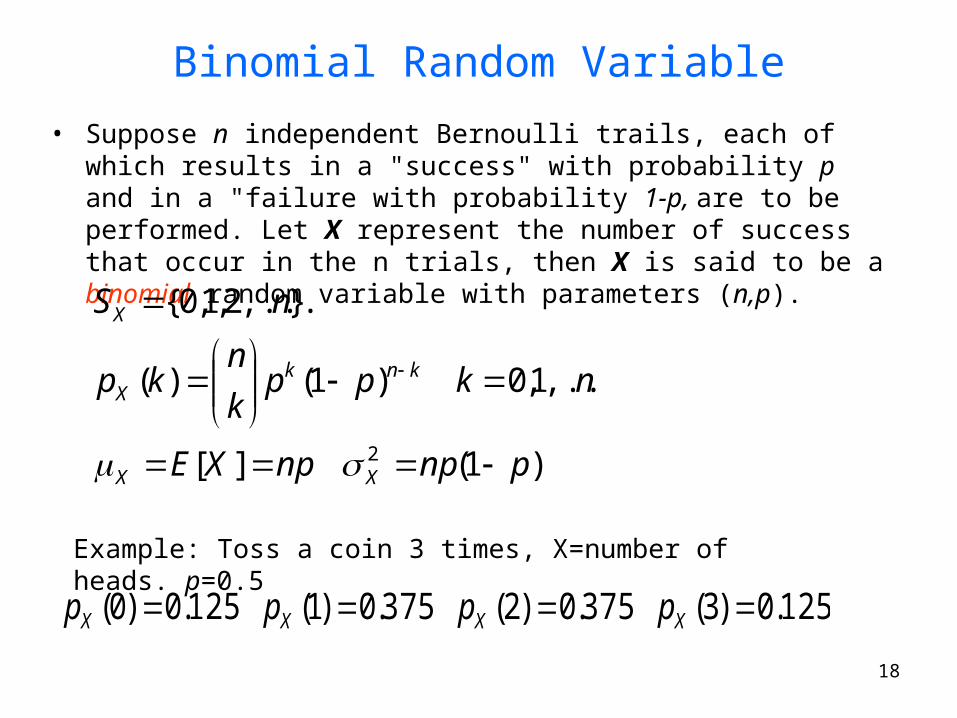
Binomial Random Variable
• Suppose n independent Bernoulli trails, each of which results in a "success" with probability p and in a "failure with probability 1-p, are to be performed. Let X represent the number of success that occur in the n trials, then X is said to be a binomial random variable with parameters (n,p).
)1(][
,...1,0)1()(
},...2,1,0{
2 pnpnpXE
nkppk
nkp
nS
XX
knkX
X
Example: Toss a coin 3 times, X=number of heads. p=0.5
125.0)3(375.0)2(375.0)1(125.0)0( XXXX pppp
19
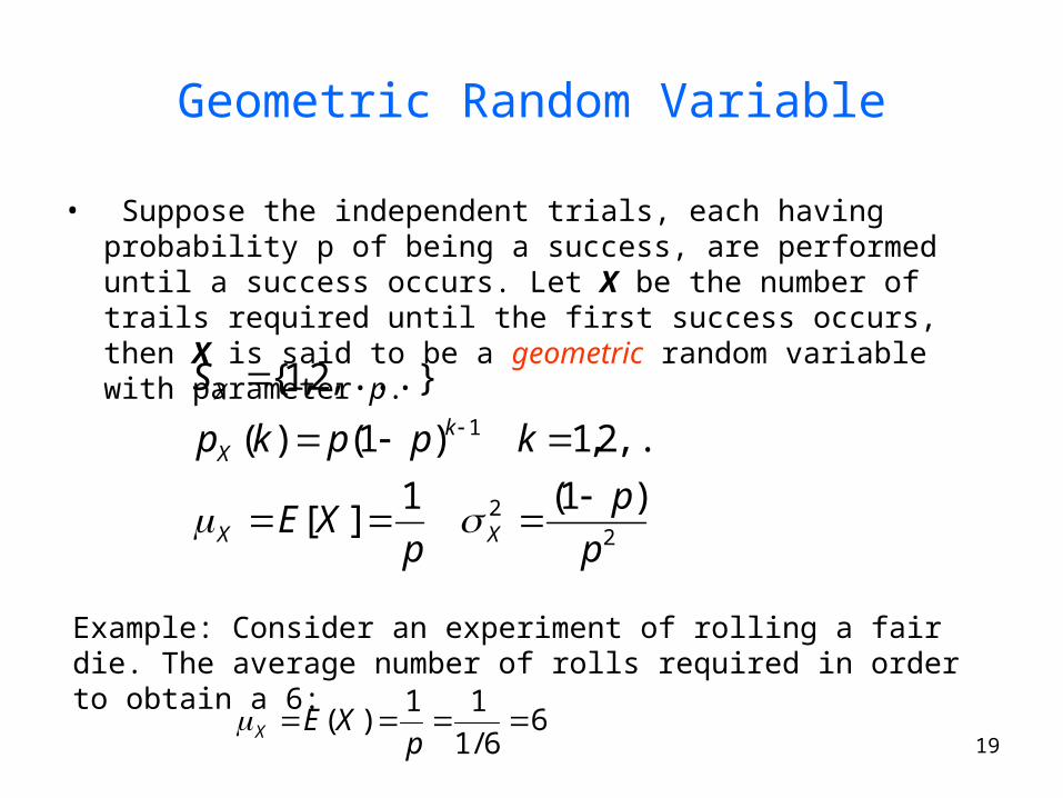
Geometric Random Variable
• Suppose the independent trials, each having probability p of being a success, are performed until a success occurs. Let X be the number of trails required until the first success occurs, then X is said to be a geometric random variable with parameter p.
22
1
)1(1][
,...2,1)1()(
,...}2,1{
p
p
pXE
kppkp
S
XX
kX
X
Example: Consider an experiment of rolling a fair die. The average number of rolls required in order to obtain a 6:
66/1
11)( p
XEX
20
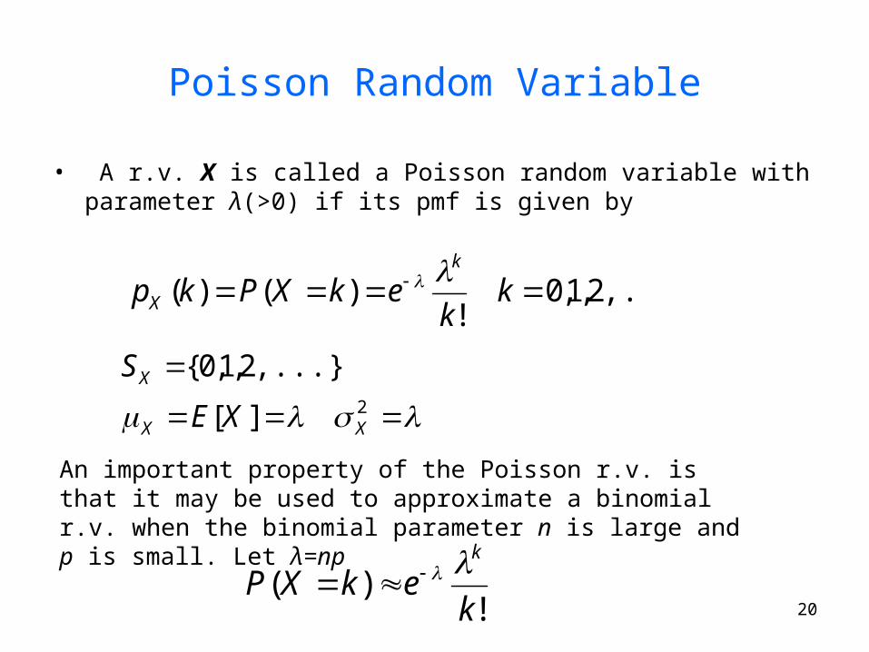
Poisson Random Variable
• A r.v. X is called a Poisson random variable with parameter λ(>0) if its pmf is given by
,...2,1,0!
)()( kk
ekXPkpk
X
2][
,...}2,1,0{
XX
X
XE
S
An important property of the Poisson r.v. is that it may be used to approximate a binomial r.v. when the binomial parameter n is large and p is small. Let λ=np
!)(
kekXP
k
21
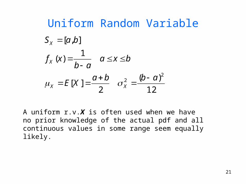
Uniform Random Variable
12
)(
2][
1)(
],[
22 abba
XE
bxaab
xf
baS
XX
X
X
A uniform r.v.X is often used when we have no prior knowledge of the actual pdf and all continuous values in some range seem equally likely.
22
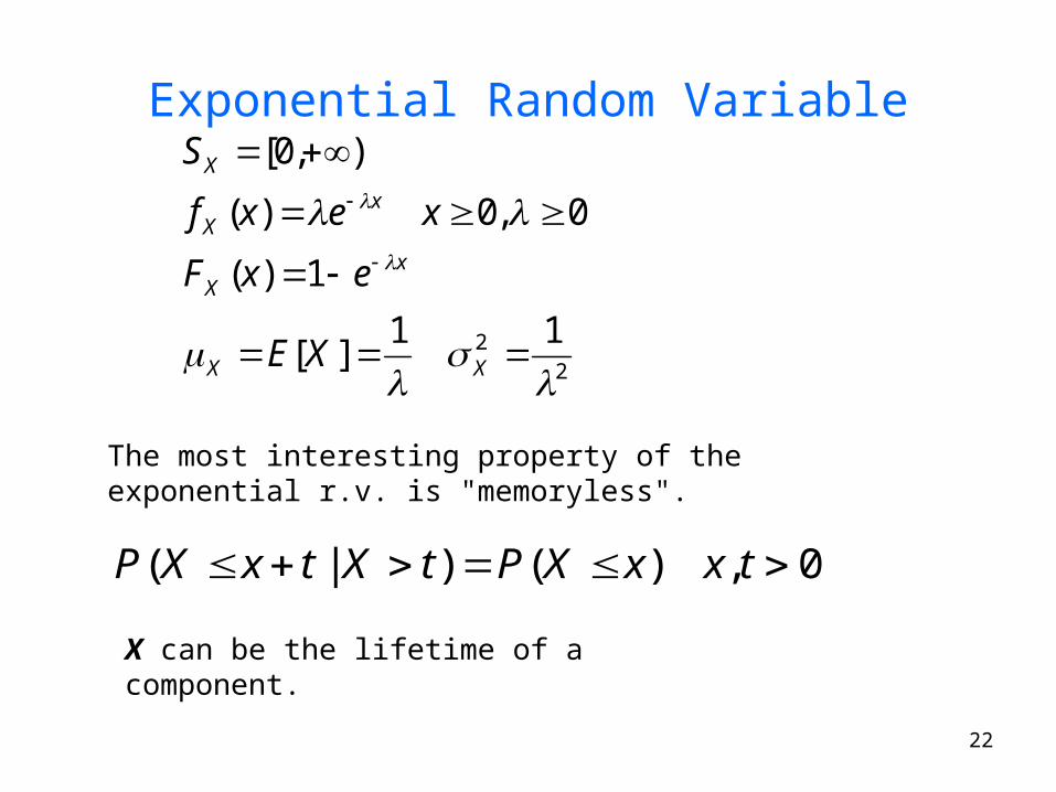
Exponential Random Variable
22 11
][
1)(
0,0)(
),0[
XX
xX
xX
X
XE
exF
xexf
S
The most interesting property of the exponential r.v. is "memoryless".
0,)()|( txxXPtXtxXP
X can be the lifetime of a component.
23
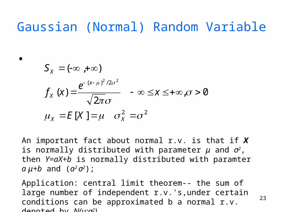
Gaussian (Normal) Random Variable
•
22
2/)(
][
0,2
)(
),(22
XX
x
X
X
XE
xe
xf
S
An important fact about normal r.v. is that if X is normally distributed with parameter μ and σ2, then Y=aX+b is normally distributed with paramter a μ+b and (a2 σ2);
Application: central limit theorem-- the sum of large number of independent r.v.'s,under certain conditions can be approximated b a normal r.v. denoted by N(μ;σ2)
24
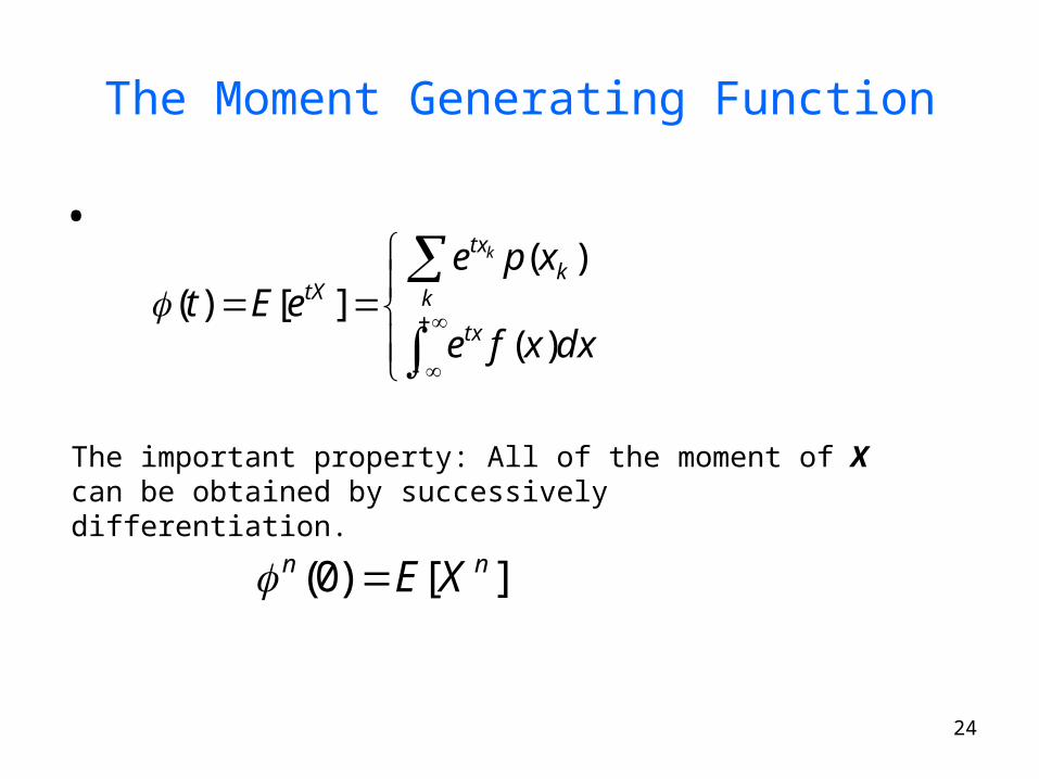
The Moment Generating Function
•
dxxfe
xpeeEt
tx
kk
tx
tX
k
)(
)(][)(
The important property: All of the moment of X can be obtained by successively differentiation.
][)0( nn XE
25
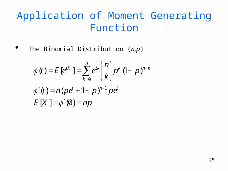
Application of Moment Generating Function
• The Binomial Distribution (n,p)
npXE
peppent
ppk
neeEt
tnt
knkn
k
tktX
)0(][
)1()(
)1(][)(
1
0
26
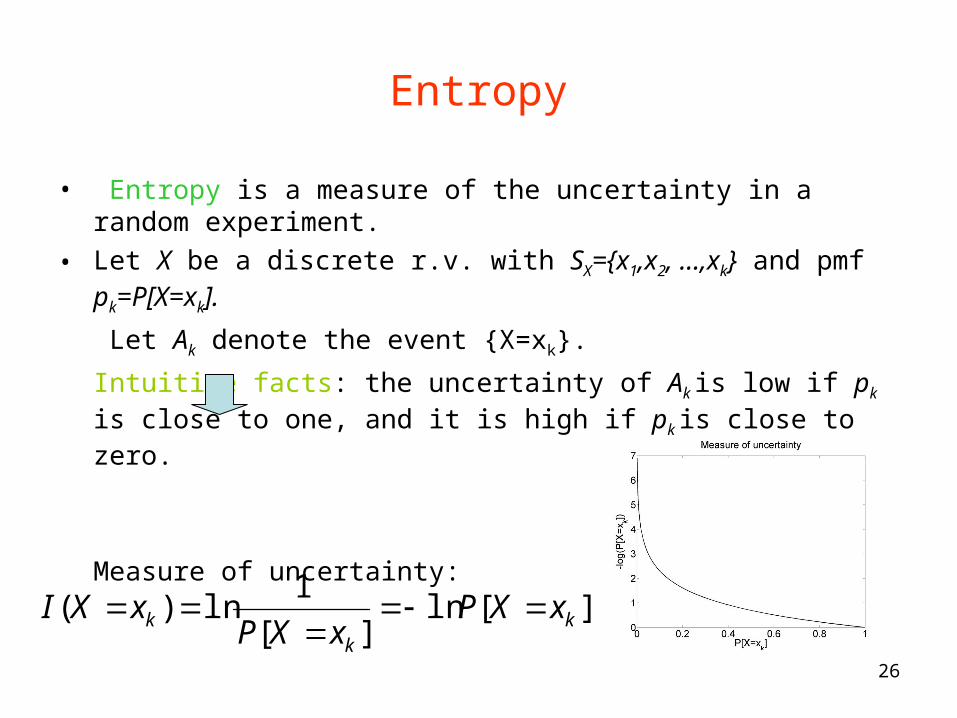
Entropy
• Entropy is a measure of the uncertainty in a random experiment.
• Let X be a discrete r.v. with SX={x1,x2, …,xk} and pmf pk=P[X=xk].
Let Ak denote the event {X=xk}.
Intuitive facts: the uncertainty of Ak is low if pk is close to one, and it is high if pk is close to zero.
Measure of uncertainty:
][ln][
1ln)( k
kk xXP
xXPxXI
27
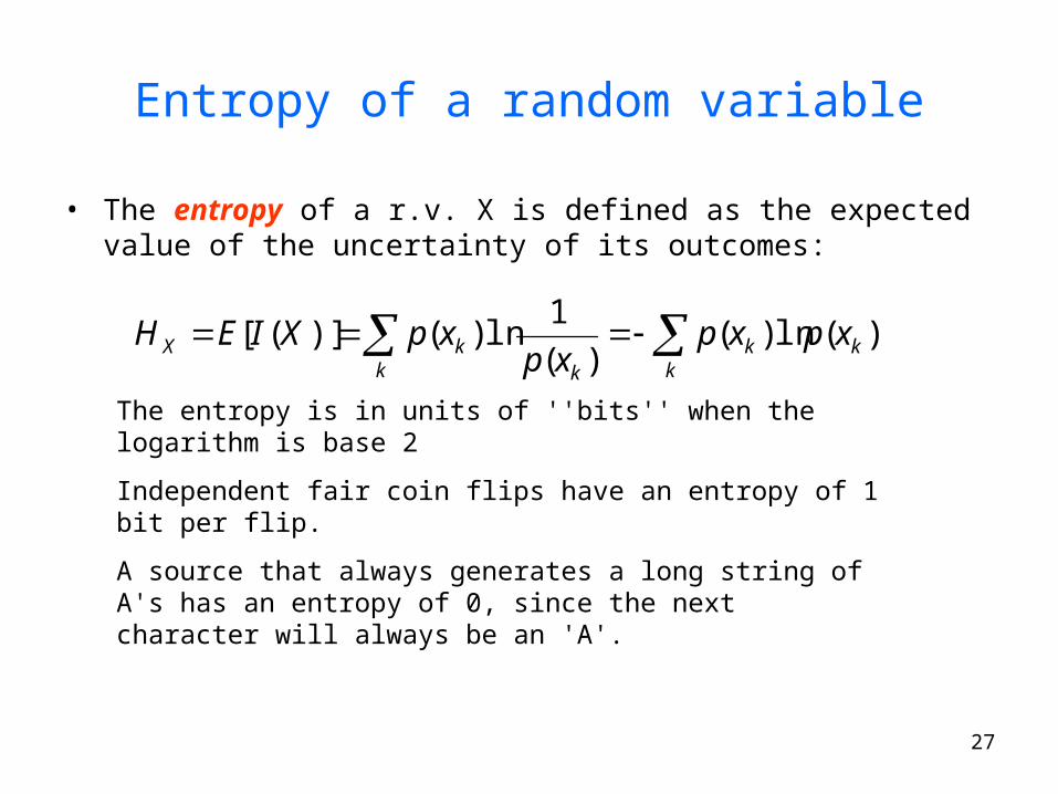
Entropy of a random variable
• The entropy of a r.v. X is defined as the expected value of the uncertainty of its outcomes:
)(ln)()(
1ln)()]([ k
kk
k kkX xpxp
xpxpXIEH
The entropy is in units of ''bits'' when the logarithm is base 2
Independent fair coin flips have an entropy of 1 bit per flip.
A source that always generates a long string of A's has an entropy of 0, since the next character will always be an 'A'.
28
Entropy of Binary Random Variable
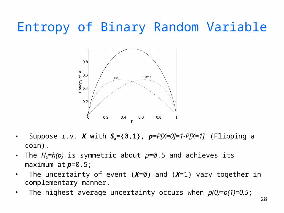
• Suppose r.v. X with Sx={0,1}, p=P[X=0]=1-P[X=1]. (Flipping a coin).
• The HX=h(p) is symmetric about p=0.5 and achieves its maximum at p=0.5;
• The uncertainty of event (X=0) and (X=1) vary together in complementary manner.
• The highest average uncertainty occurs when p(0)=p(1)=0.5;
29
Reduction of Entropy Through Partial Information
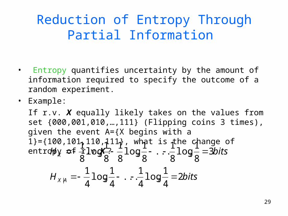
• Entropy quantifies uncertainty by the amount of information required to specify the outcome of a random experiment.
• Example:
If r.v. X equally likely takes on the values from set {000,001,010,…,111} (Flipping coins 3 times), given the event A={X begins with a 1}={100,101,110,111}, what is the change of entropy of r.v.X ?
bitsH
bitsH
AX
X
24
1log4
1...
4
1log4
1
38
1log8
1...
8
1log8
1
8
1log8
1
22|
222

30
Thanks! Question?
31
Extending discrete entropy to the continuous
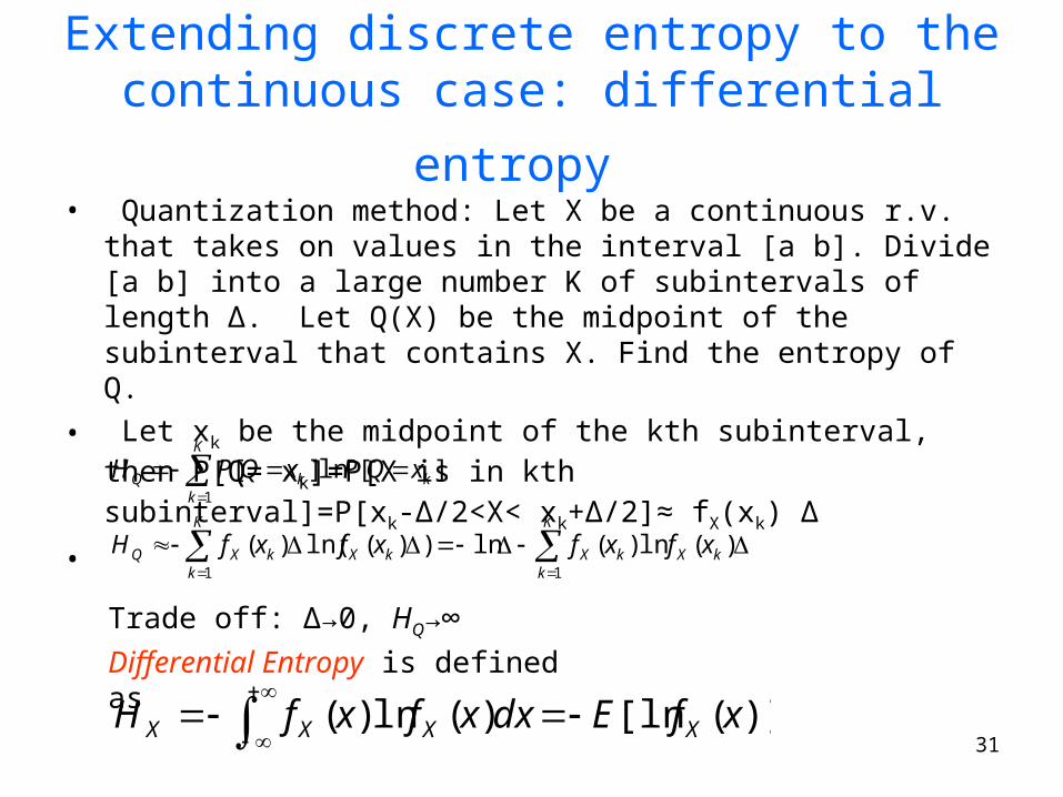
case: differential entropy • Quantization method: Let X be a continuous r.v. that takes on
values in the interval [a b]. Divide [a b] into a large number K of subintervals of length ∆. Let Q(X) be the midpoint of the subinterval that contains X. Find the entropy of Q.
• Let xk be the midpoint of the kth subinterval, then P[Q= xk]=P[X is in kth subinterval]=P[xk-∆/2<X< xk+∆/2]≈ fX(xk) ∆
•
K
kkXkX
K
kkXkXQ
K
kkkQ
xfxfxfxfH
xQPxQPH
11
1
)(ln)(ln))(ln()(
][ln][
Trade off: ∆→0, HQ→∞
)]([ln)(ln)( xfEdxxfxfH XXXX
Differential Entropy is defined as
32
The Method of Maximum Entropy
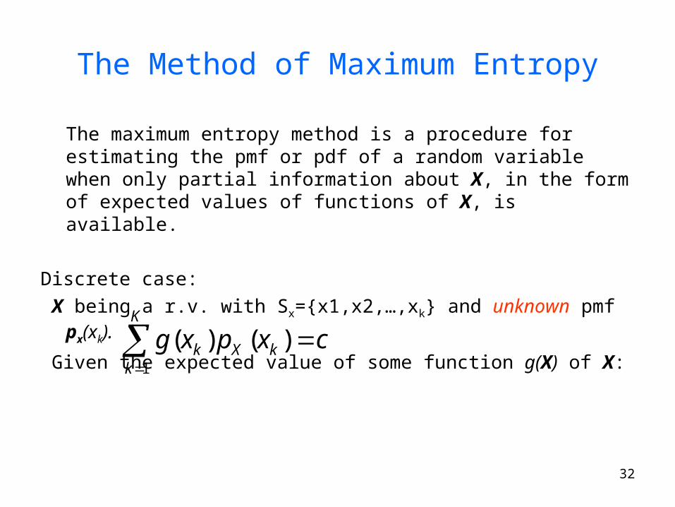
The maximum entropy method is a procedure for estimating the pmf or pdf of a random variable when only partial information about X, in the form of expected values of functions of X, is available.
Discrete case:
X being a r.v. with Sx={x1,x2,…,xk} and unknown pmf px(xk).
Given the expected value of some function g(X) of X:
cxpxg k
K
kXk
)()(1


![1 Appendix: Common distributionsfaculty.chicagobooth.edu/nicholas.polson/teaching/41900/Appendices...1 Appendix: Common distributions ... Beta • A random variable X ∈ [0,1] has](https://static.fdocument.org/doc/165x107/5ae3e1407f8b9a595d8f03f5/1-appendix-common-appendix-common-distributions-beta-a-random-variable.jpg)