ΔΙΑΧΕΙΡΙΣΗ ΔΙΚΤΥΩΝΔΙΑΧΕΙΡΙΣΗ ΔΙΚΤΥΩΝ

ΔΡΟΜΟΛΟΓΗΣΗ ΣΤΟ ΔΙΑΔΙΚΤΥΟ - ΑΛΓΟΡΙΘΜΟΙ

Συμεών Παπαβασιλείουpapavass@mail.ntua.gr

12/11/2012

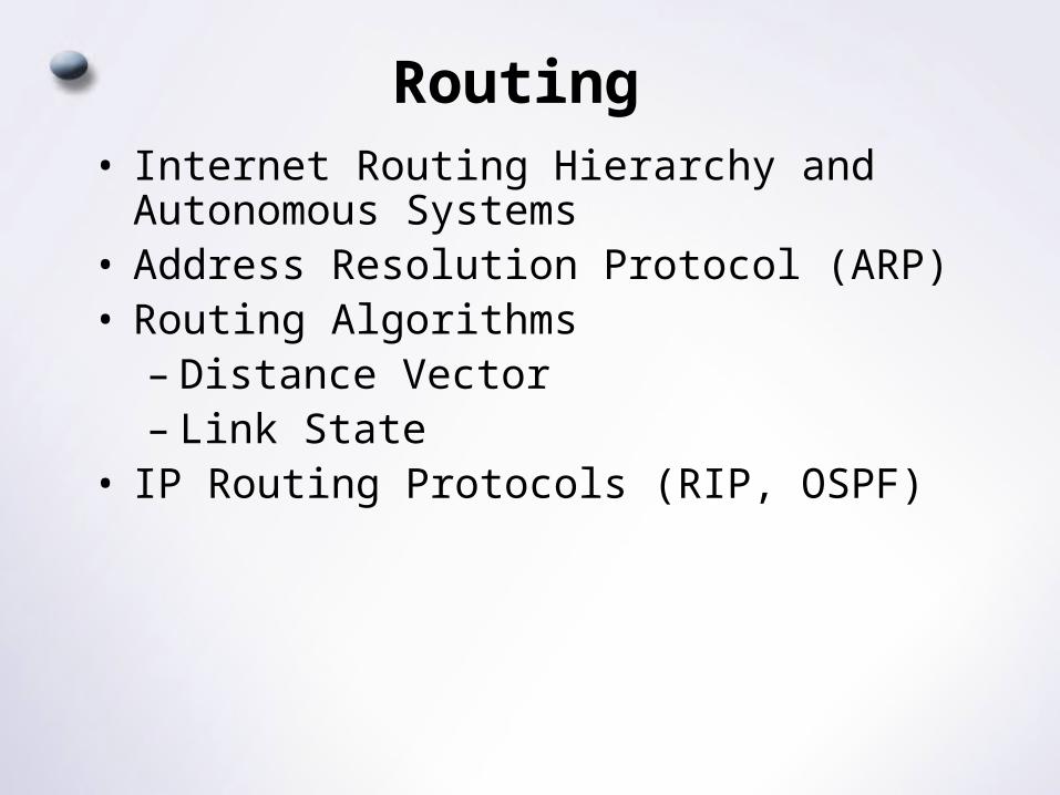
Routing • Internet Routing Hierarchy and Autonomous

Systems• Address Resolution Protocol (ARP)• Routing Algorithms

– Distance Vector– Link State

• IP Routing Protocols (RIP, OSPF)

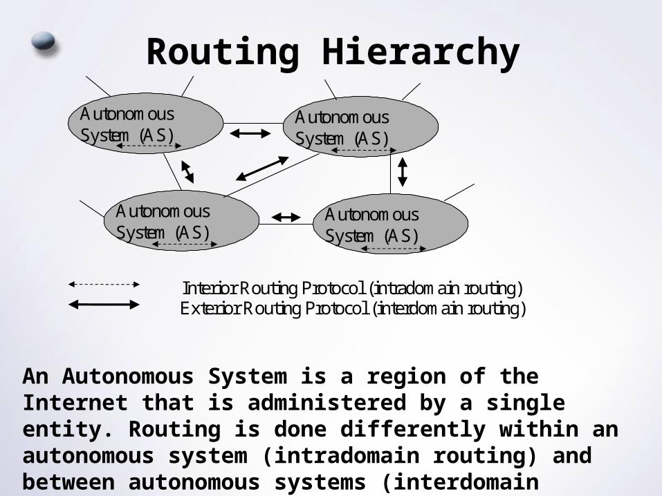
Routing Hierarchy

AutonomousSystem (AS)

AutonomousSystem (AS)

AutonomousSystem (AS)

AutonomousSystem (AS)

Exterior Routing Protocol (interdomain routing)Interior Routing Protocol (intradomain routing)

An Autonomous System is a region of the Internet that is administered by a single entity. Routing is done differently within an autonomous system (intradomain routing) and between autonomous systems (interdomain routing)

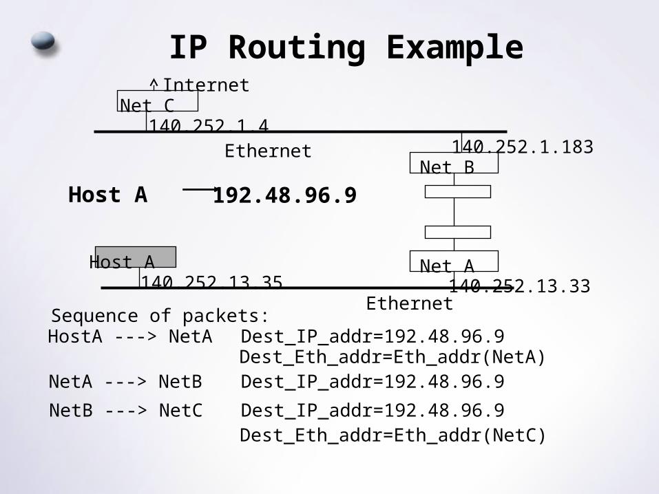
IP Routing Example

Ethernet

Host A Net A

Net B

Net CInternet

Ethernet

140.252.13.35 140.252.13.33

140.252.1.183140.252.1.4

Host A 192.48.96.9

Sequence of packets:HostA ---> NetA Dest_IP_addr=192.48.96.9

Dest_Eth_addr=Eth_addr(NetA)NetA ---> NetB Dest_IP_addr=192.48.96.9

NetB ---> NetC Dest_IP_addr=192.48.96.9Dest_Eth_addr=Eth_addr(NetC)

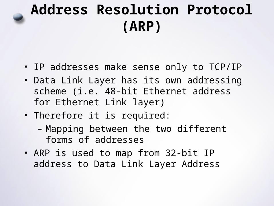
Address Resolution Protocol (ARP)

• IP addresses make sense only to TCP/IP• Data Link Layer has its own addressing scheme (i.e.

48-bit Ethernet address for Ethernet Link layer)• Therefore it is required:

– Mapping between the two different forms of addresses

• ARP is used to map from 32-bit IP address to Data Link Layer Address

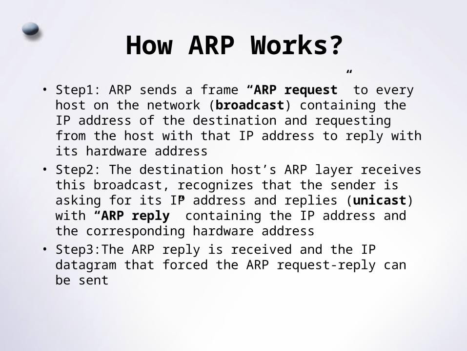
How ARP Works?

• Step1: ARP sends a frame “ARP request” to every host on the network (broadcast) containing the IP address of the destination and requesting from the host with that IP address to reply with its hardware address

• Step2: The destination host’s ARP layer receives this broadcast, recognizes that the sender is asking for its IP address and replies (unicast) with “ARP reply” containing the IP address and the corresponding hardware address

• Step3:The ARP reply is received and the IP datagram that forced the ARP request-reply can be sent

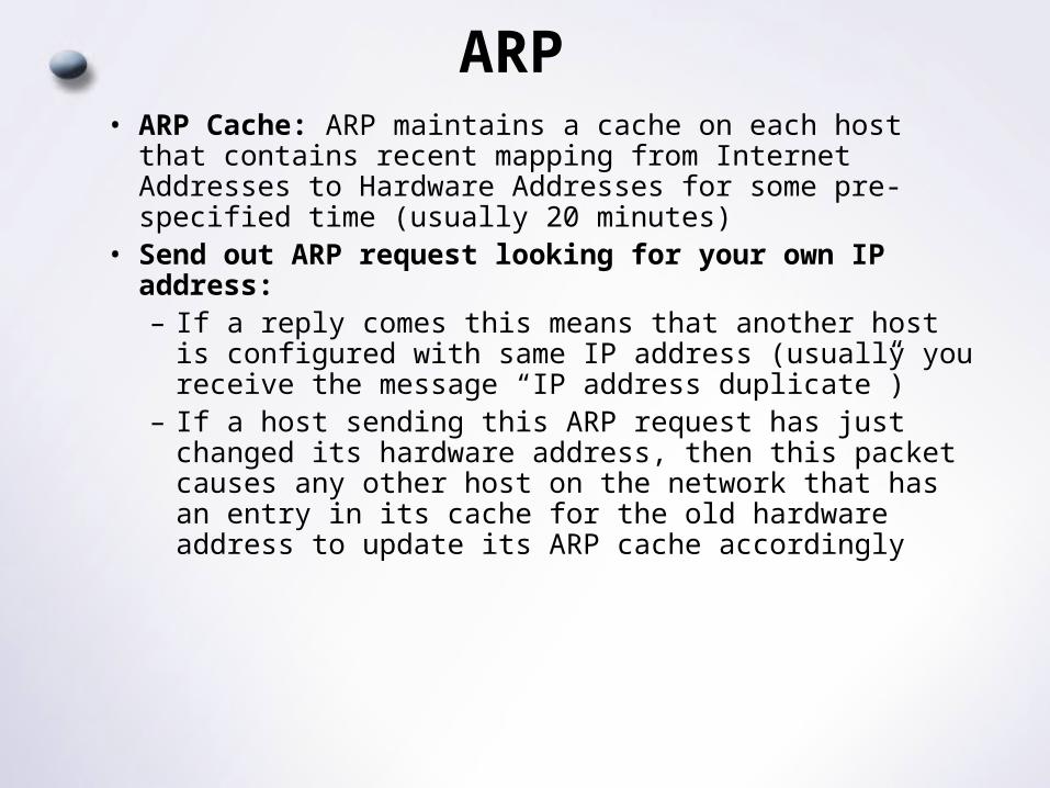
ARP • ARP Cache: ARP maintains a cache on each host that

contains recent mapping from Internet Addresses to Hardware Addresses for some pre-specified time (usually 20 minutes)

• Send out ARP request looking for your own IP address: – If a reply comes this means that another host is configured

with same IP address (usually you receive the message “IP address duplicate”)

– If a host sending this ARP request has just changed its hardware address, then this packet causes any other host on the network that has an entry in its cache for the old hardware address to update its ARP cache accordingly

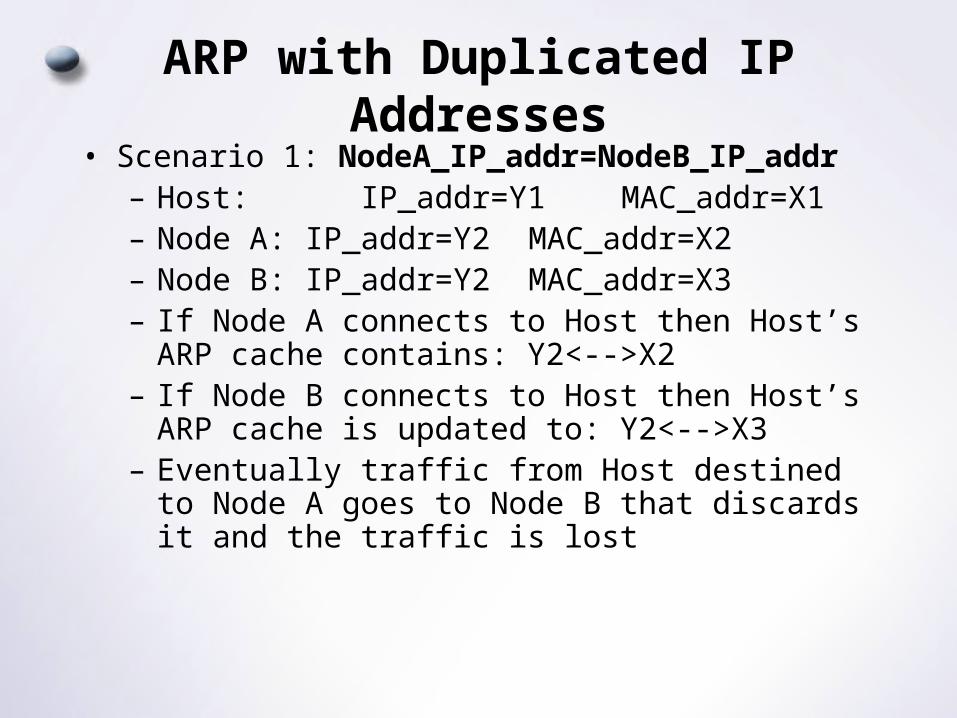
ARP with Duplicated IP Addresses• Scenario 1: NodeA_IP_addr=NodeB_IP_addr

– Host: IP_addr=Y1 MAC_addr=X1– Node A: IP_addr=Y2 MAC_addr=X2– Node B: IP_addr=Y2 MAC_addr=X3– If Node A connects to Host then Host’s ARP cache

contains: Y2<-->X2– If Node B connects to Host then Host’s ARP cache

is updated to: Y2<-->X3– Eventually traffic from Host destined to Node A

goes to Node B that discards it and the traffic is lost

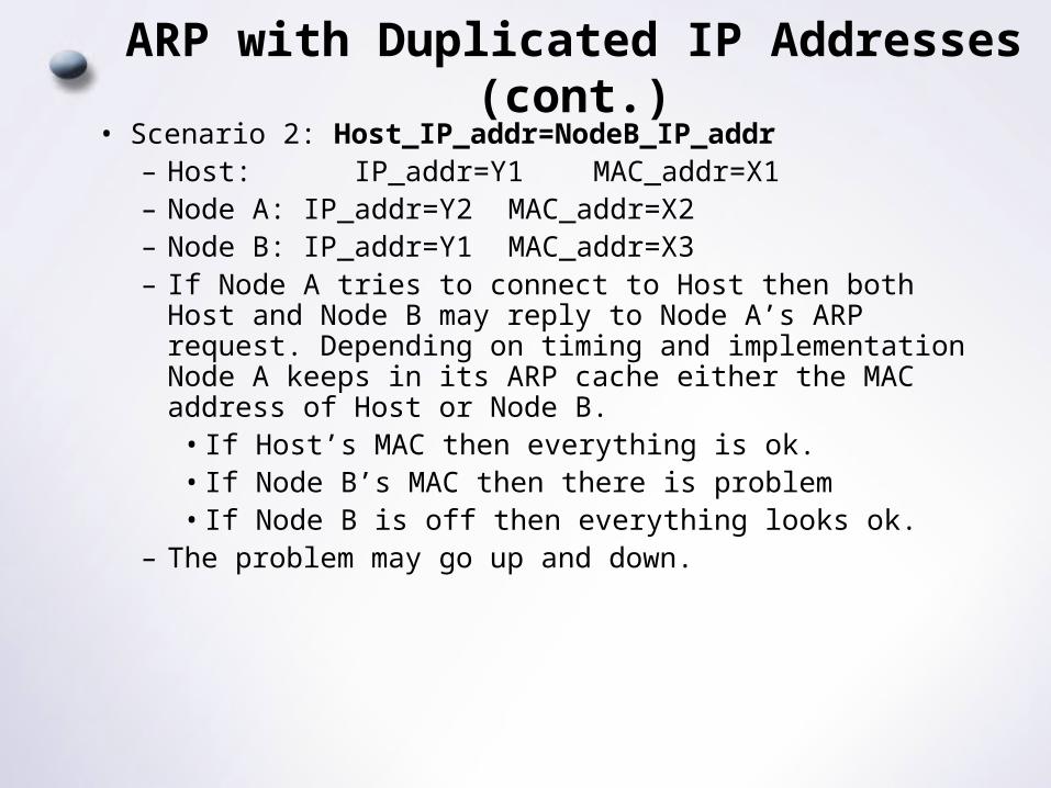
ARP with Duplicated IP Addresses (cont.)• Scenario 2: Host_IP_addr=NodeB_IP_addr

– Host: IP_addr=Y1 MAC_addr=X1– Node A: IP_addr=Y2 MAC_addr=X2– Node B: IP_addr=Y1 MAC_addr=X3– If Node A tries to connect to Host then both Host and

Node B may reply to Node A’s ARP request. Depending on timing and implementation Node A keeps in its ARP cache either the MAC address of Host or Node B.

• If Host’s MAC then everything is ok.• If Node B’s MAC then there is problem• If Node B is off then everything looks ok.

– The problem may go up and down.

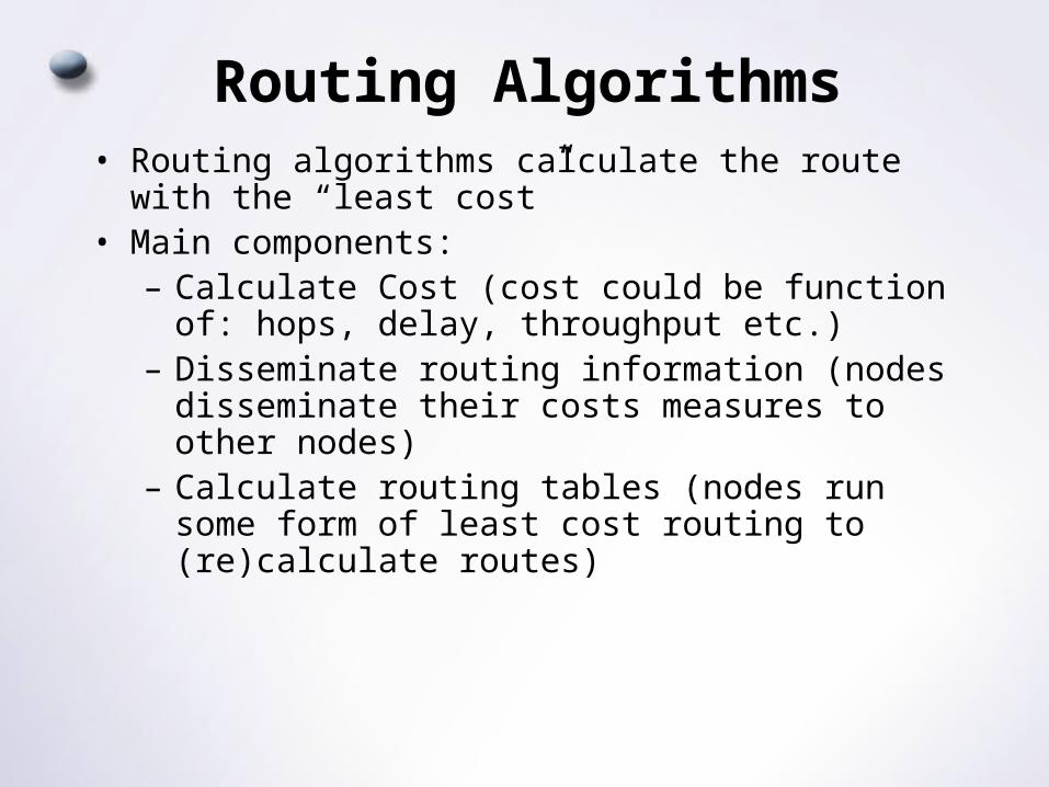
Routing Algorithms• Routing algorithms calculate the route with the “least

cost”• Main components:

– Calculate Cost (cost could be function of: hops, delay, throughput etc.)

– Disseminate routing information (nodes disseminate their costs measures to other nodes)

– Calculate routing tables (nodes run some form of least cost routing to (re)calculate routes)

Routing Protocols• Routers need to understand the topology of the network

in order to route packets properly• Routers need to tell to each other which paths are “up”

and what costs are involved• Routers communicate with each other using routing

protocols• Two broad classes of routing policies:

– Static: All routes are listed explicitly; the router does not communicate with other routers

– Dynamic: routing protocols are used to enable routers to react to changes in network topology without manual intervention

Static Routing

• When an interface is initialized the direct routes are automatically created

• Routes to hosts and networks not directly connected must be entered in the routing table (i.e. manually by command route, e.g. route add host_A router_B)

• Static routing is good in small networks• Networks should usually not mix static and dynamic

routing– Dynamic routing information may conflict with static

routing– Point-to-point links may be routed with static routes

ICMP Redirect Messages

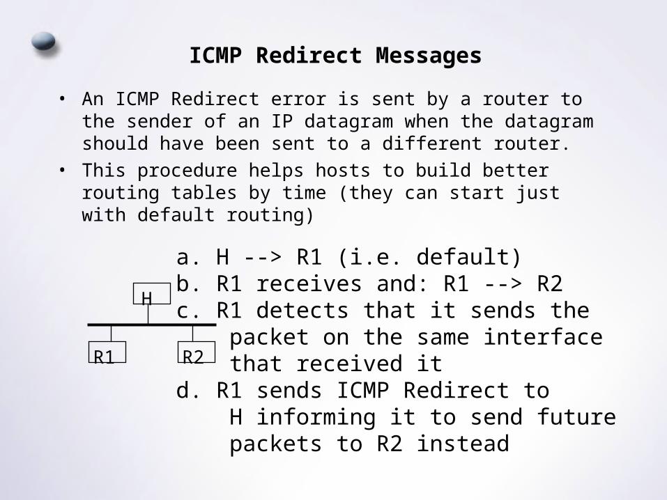
• An ICMP Redirect error is sent by a router to the sender of an IP datagram when the datagram should have been sent to a different router.

• This procedure helps hosts to build better routing tables by time (they can start just with default routing)

H

R1 R2

a. H --> R1 (i.e. default)b. R1 receives and: R1 --> R2c. R1 detects that it sends the packet on the same interface that received itd. R1 sends ICMP Redirect to H informing it to send future packets to R2 instead

Dynamic Routing Protocols• Two classes of dynamic routing protocols• Distance Vector (DV): Routers know local

information and broadcast it to other neighboring routers– Each node knows the distance to all other nodes– A node sends a list to its neighbors with the

shortest distances to all nodes– If all nodes update their distances, the routing

tables eventually converge

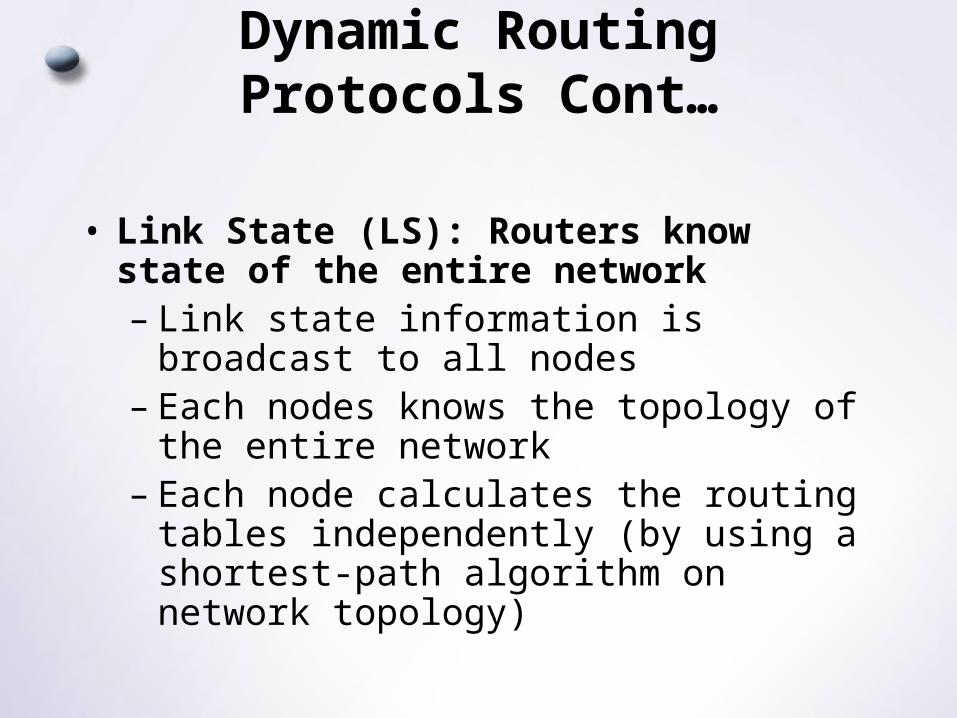
Dynamic Routing Protocols Cont…

• Link State (LS): Routers know state of the entire network– Link state information is broadcast to all

nodes– Each nodes knows the topology of the

entire network– Each node calculates the routing tables

independently (by using a shortest-path algorithm on network topology)

Parameters

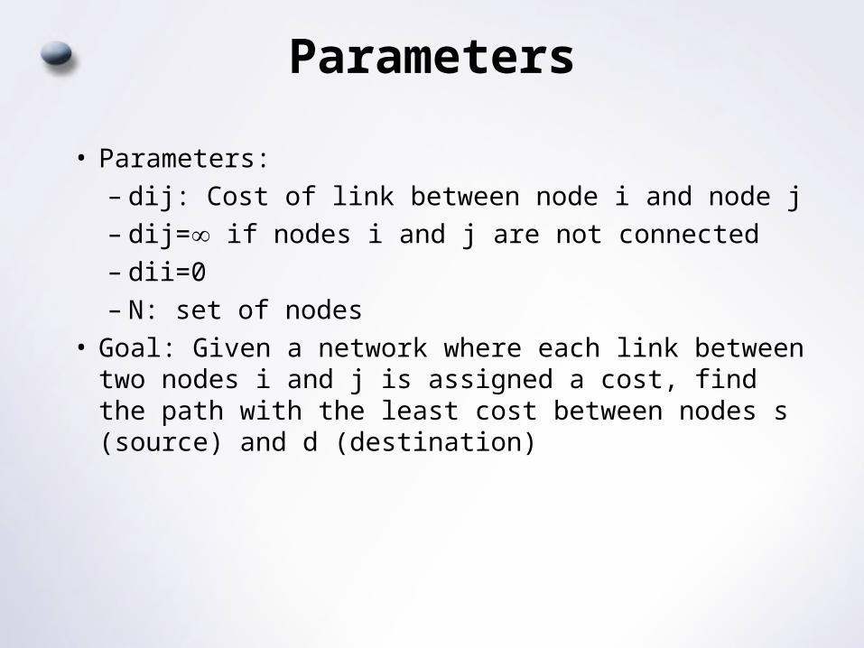
• Parameters:– dij: Cost of link between node i and node j– dij= if nodes i and j are not connected– dii=0– N: set of nodes

• Goal: Given a network where each link between two nodes i and j is assigned a cost, find the path with the least cost between nodes s (source) and d (destination)

Network Example

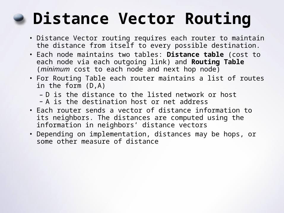
Distance Vector Routing• Distance Vector routing requires each router to maintain the

distance from itself to every possible destination.• Each node maintains two tables: Distance table (cost to each node

via each outgoing link) and Routing Table (minimum cost to each node and next hop node)

• For Routing Table each router maintains a list of routes in the form (D,A)– D is the distance to the listed network or host – A is the destination host or net address

• Each router sends a vector of distance information to its neighbors. The distances are computed using the information in neighbors’ distance vectors

• Depending on implementation, distances may be hops, or some other measure of distance

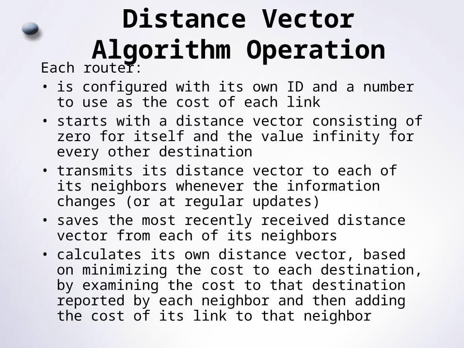
Distance Vector Algorithm Operation

Each router:• is configured with its own ID and a number to use as

the cost of each link• starts with a distance vector consisting of zero for

itself and the value infinity for every other destination• transmits its distance vector to each of its neighbors

whenever the information changes (or at regular updates)

• saves the most recently received distance vector from each of its neighbors

• calculates its own distance vector, based on minimizing the cost to each destination, by examining the cost to that destination reported by each neighbor and then adding the cost of its link to that neighbor

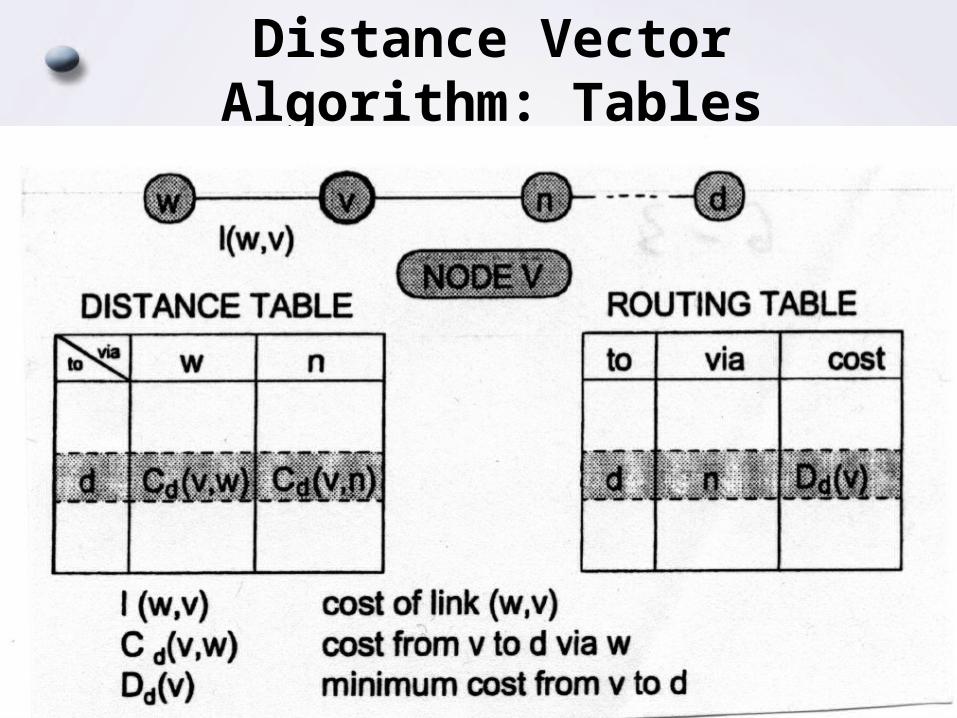
Distance Vector Algorithm: Tables

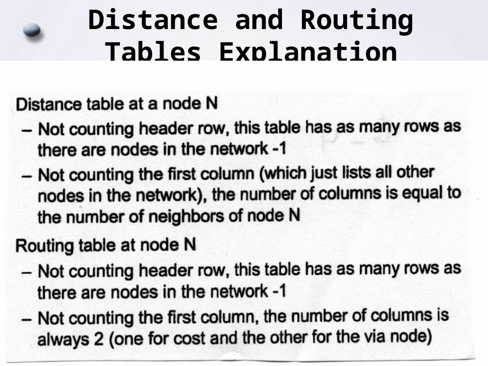
Distance and Routing Tables Explanation

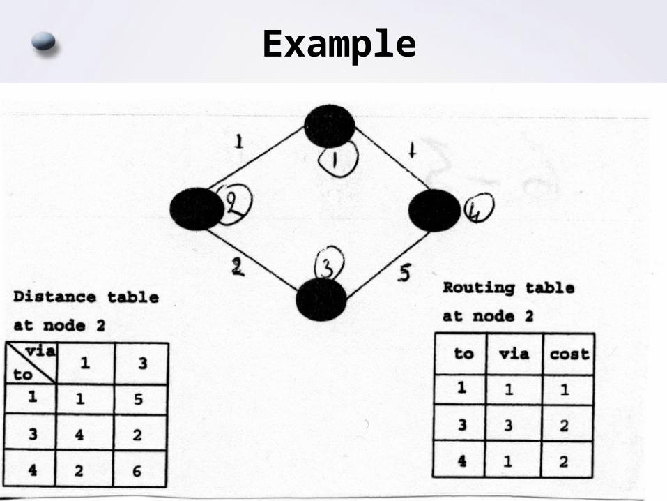
Example

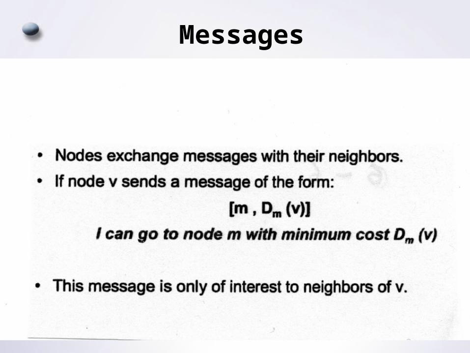
Messages

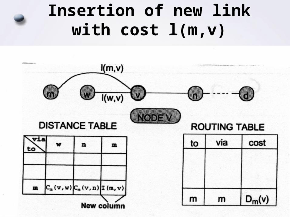
Insertion of new link with cost l(m,v)

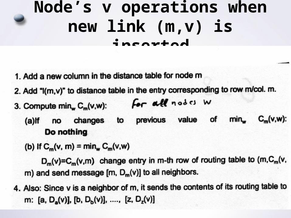
Node’s v operations when new link (m,v) is inserted

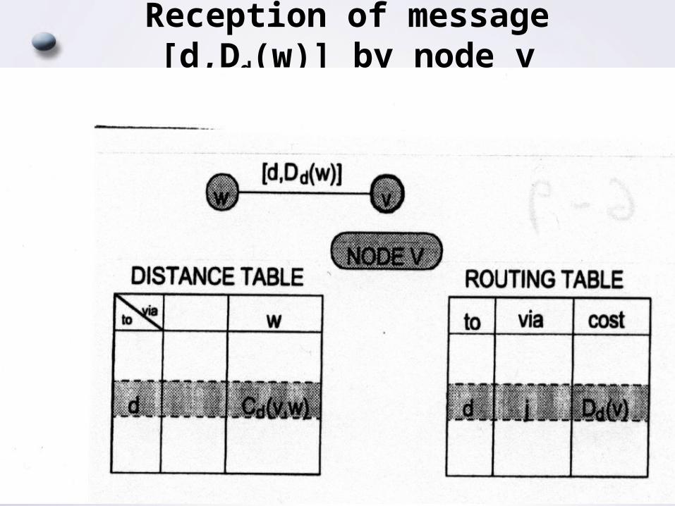
Reception of message [d,Dd(w)] by node v

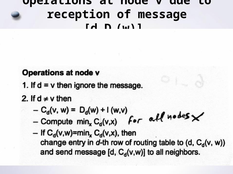
Operations at node v due to reception of message [d,Dd(w)]

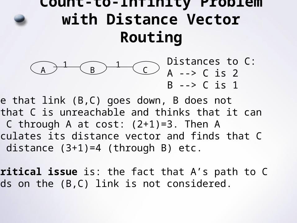
Count-to-Infinity Problem with Distance Vector Routing

A B C1 1 Distances to C:

A --> C is 2B --> C is 1

Assume that link (B,C) goes down, B does notknow that C is unreachable and thinks that it canreach C through A at cost: (2+1)=3. Then A recalculates its distance vector and finds that Cis at distance (3+1)=4 (through B) etc.

The critical issue is: the fact that A’s path to Cdepends on the (B,C) link is not considered.

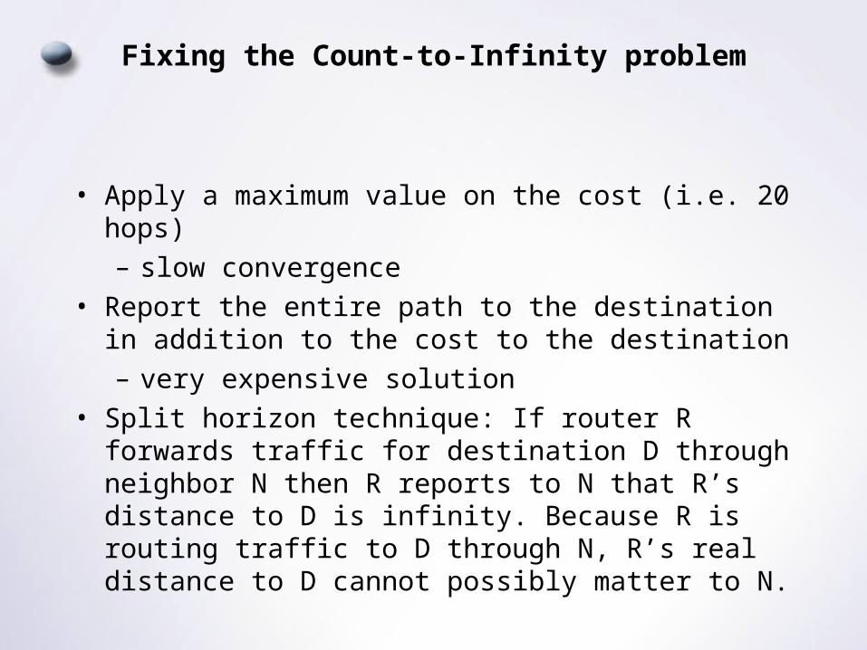
Fixing the Count-to-Infinity problem

• Apply a maximum value on the cost (i.e. 20 hops) – slow convergence

• Report the entire path to the destination in addition to the cost to the destination– very expensive solution

• Split horizon technique: If router R forwards traffic for destination D through neighbor N then R reports to N that R’s distance to D is infinity. Because R is routing traffic to D through N, R’s real distance to D cannot possibly matter to N.

Link State Routing

• Link State routing is an alternative to Distance Vector routing

• Link State routers do not exchange distance information as Distance Vector routers.

• They only exchange the state of the link to each neighbor

• OSPF (Open Shortest Path First) is the most popular link state routing algorithm in IP

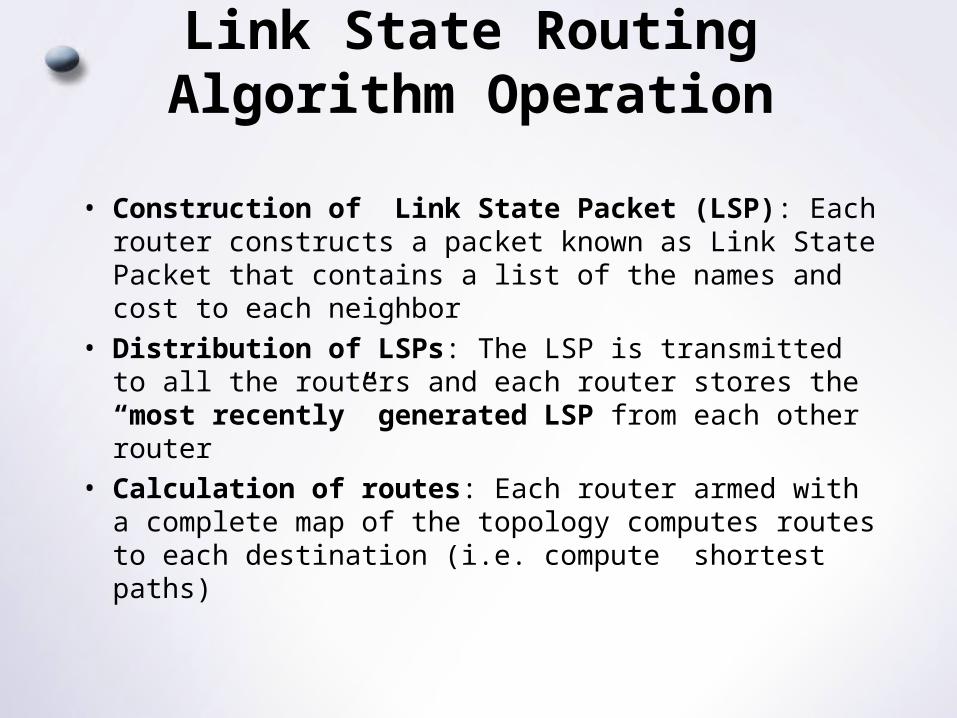
Link State Routing Algorithm Operation

• Construction of Link State Packet (LSP): Each router constructs a packet known as Link State Packet that contains a list of the names and cost to each neighbor

• Distribution of LSPs: The LSP is transmitted to all the routers and each router stores the “most recently” generated LSP from each other router

• Calculation of routes: Each router armed with a complete map of the topology computes routes to each destination (i.e. compute shortest paths)

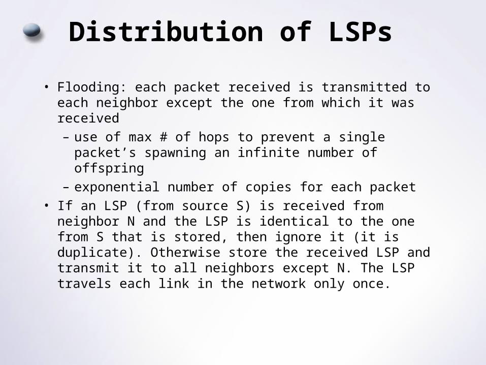
Distribution of LSPs

• Flooding: each packet received is transmitted to each neighbor except the one from which it was received– use of max # of hops to prevent a single packet’s

spawning an infinite number of offspring– exponential number of copies for each packet

• If an LSP (from source S) is received from neighbor N and the LSP is identical to the one from S that is stored, then ignore it (it is duplicate). Otherwise store the received LSP and transmit it to all neighbors except N. The LSP travels each link in the network only once.

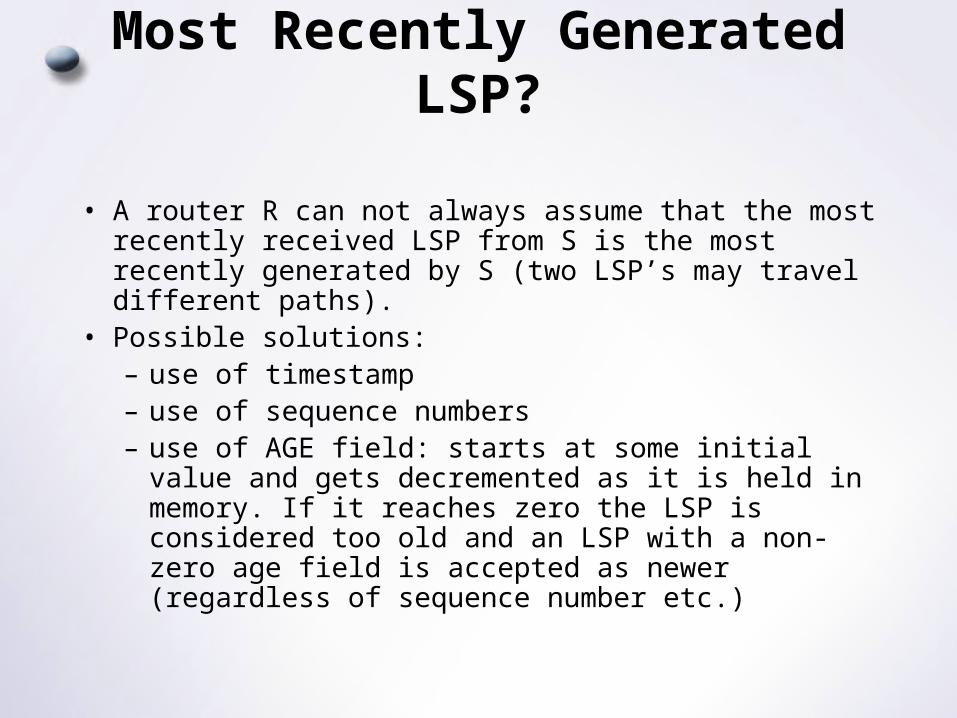
Most Recently Generated LSP?

• A router R can not always assume that the most recently received LSP from S is the most recently generated by S (two LSP’s may travel different paths).

• Possible solutions:– use of timestamp– use of sequence numbers– use of AGE field: starts at some initial value and

gets decremented as it is held in memory. If it reaches zero the LSP is considered too old and an LSP with a non-zero age field is accepted as newer (regardless of sequence number etc.)

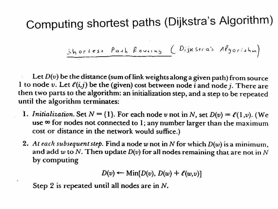
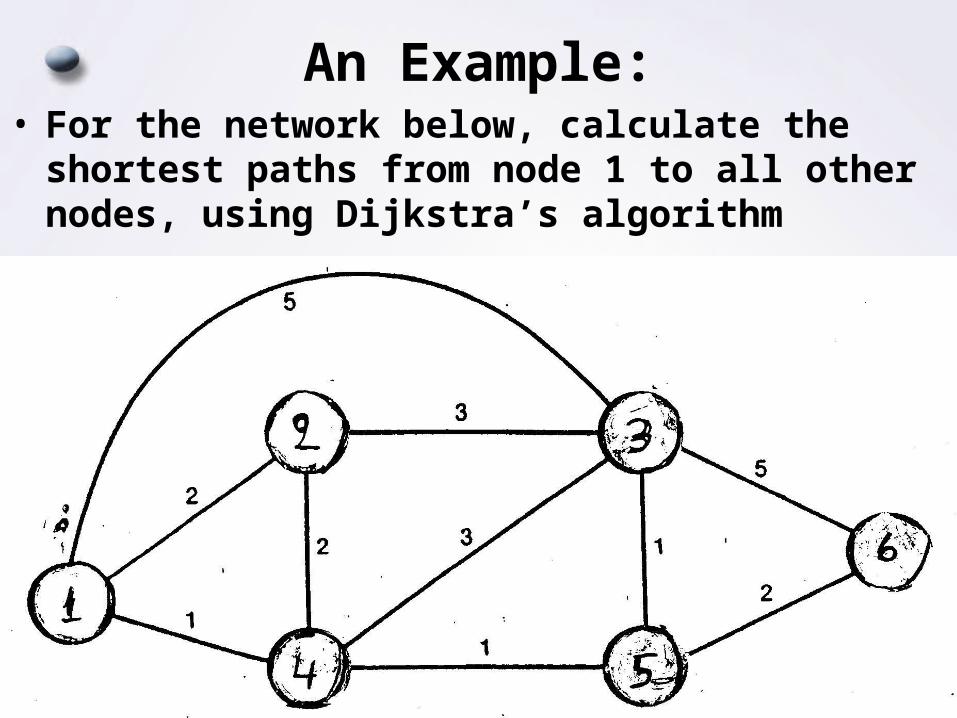
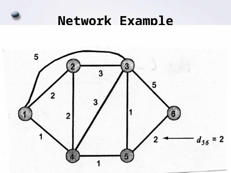
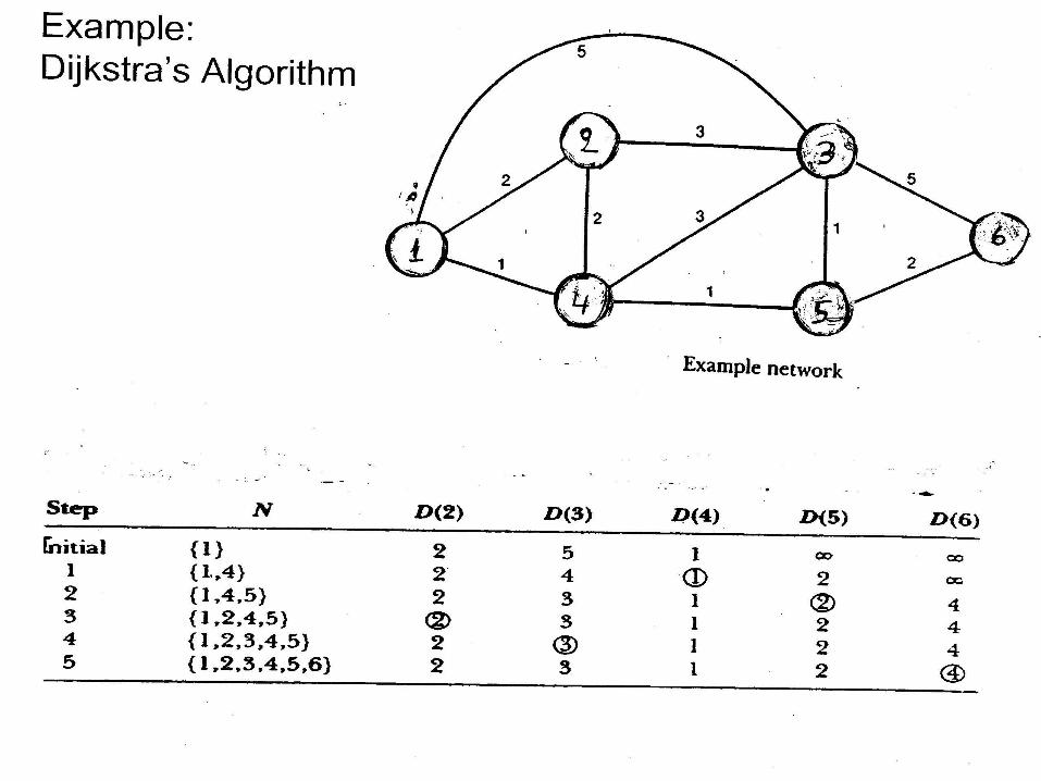
An Example:• For the network below, calculate the shortest

paths from node 1 to all other nodes, using Dijkstra’s algorithm

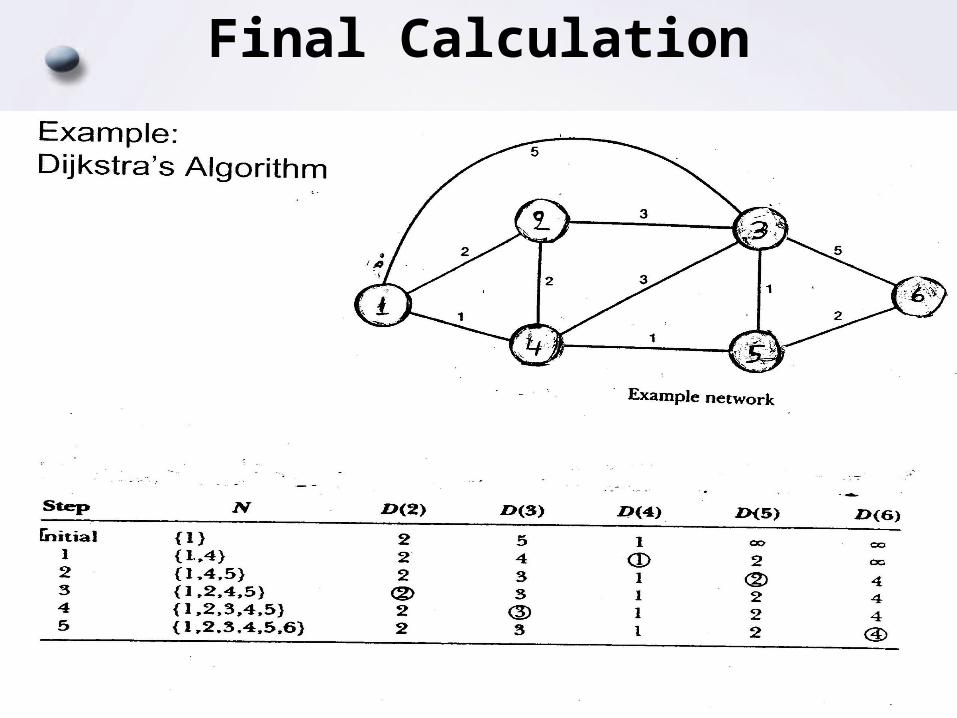
Final Calculation

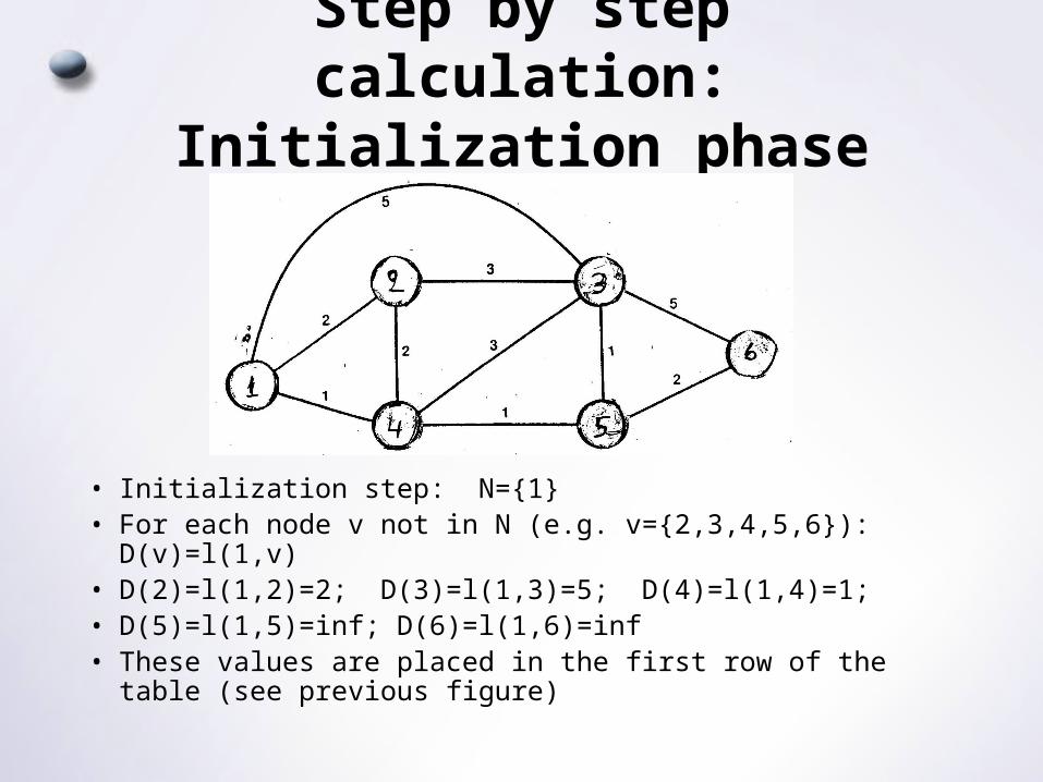
Step by step calculation:Initialization phase

• Initialization step: N={1}• For each node v not in N (e.g. v={2,3,4,5,6}): D(v)=l(1,v)• D(2)=l(1,2)=2; D(3)=l(1,3)=5; D(4)=l(1,4)=1; • D(5)=l(1,5)=inf; D(6)=l(1,6)=inf• These values are placed in the first row of the table (see

previous figure)

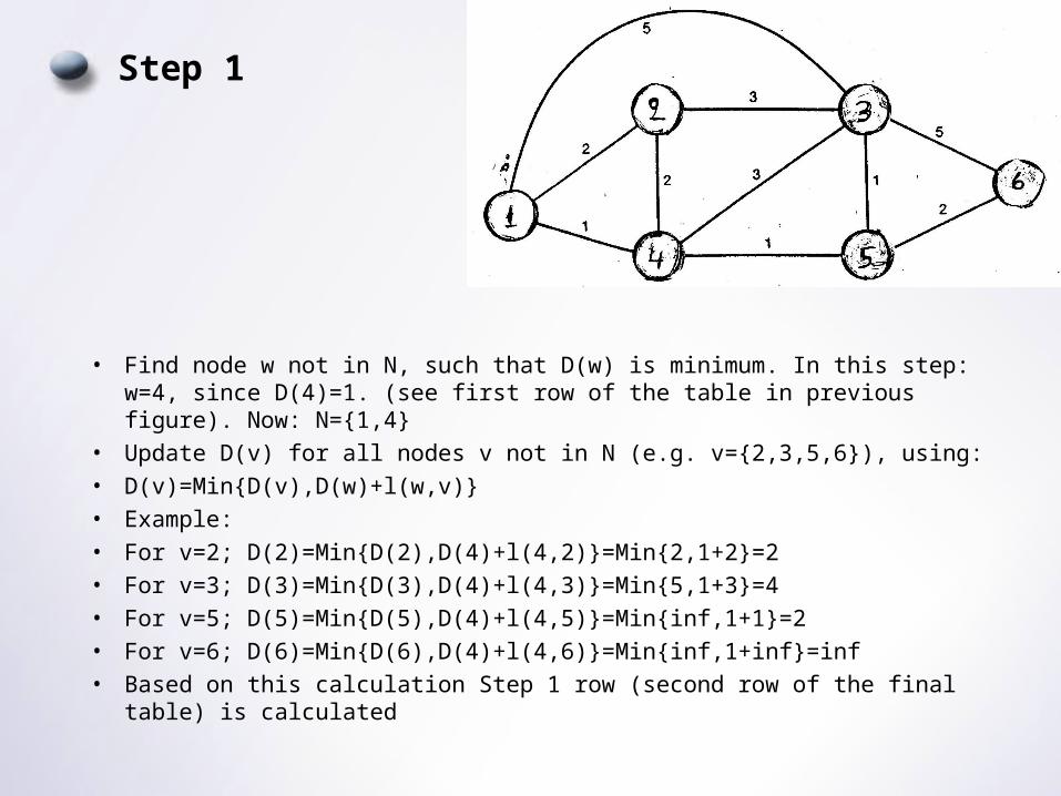
Step 1

• Find node w not in N, such that D(w) is minimum. In this step: w=4, since D(4)=1. (see first row of the table in previous figure). Now: N={1,4}

• Update D(v) for all nodes v not in N (e.g. v={2,3,5,6}), using:

• D(v)=Min{D(v),D(w)+l(w,v)}

• Example:

• For v=2; D(2)=Min{D(2),D(4)+l(4,2)}=Min{2,1+2}=2

• For v=3; D(3)=Min{D(3),D(4)+l(4,3)}=Min{5,1+3}=4

• For v=5; D(5)=Min{D(5),D(4)+l(4,5)}=Min{inf,1+1}=2

• For v=6; D(6)=Min{D(6),D(4)+l(4,6)}=Min{inf,1+inf}=inf

• Based on this calculation Step 1 row (second row of the final table) is calculated

Following steps

• Same procedure as before is repeated in order to obtain the new updated calculation (Step 2 row in the final table). In step 2 we have to find node w not in N, such that D(w) is minimum (see second row on the table). In this step we choose: w=5, since D(5)=2. Please note that D(2)=D(5)=2 in this step. In the case of tie as here, among those nodes that tie, we choose one node randomly. Here we chose w=5. Therefore: N={1,4,5}.

• In this step we update D(v) for all nodes v not in N (e.g. v={2,3,6}), using: D(v)=Min{D(v),D(w)+l(w,v)}. After completing this step, Step 2 row (third row in the final table) is completed, and so on, until you exhaust all the nodes..

Comparison of Link State and Distance Vector Routing

• Memory: Assume n-nodes in the network and that each node has k-neighbors:– Distance Vector: Each DV is O(n)and keeps

distance vector from each of its k neighbors. Therefore O(k x n).

– Link State: Each node keeps n LSPs (one from each node in the network). Each LSP is proportional to k. Therefore: O(n x k).

• Bandwidth Consumption: Depends heavily on the topology.

Comparison of Link State and Distance Vector Routing (cont.)

– Distance Vector fans: a link change only propagates control messages as far as the link change’s routing effect (i.e. in case of two parallel links where one fails and recovers)

– Link Sate fans:a link change can cause the transmission of multiple control packets over a single link under distance Vector (i.e. count to infinity problem. Under LS each LSP travels only once on each link.

• Speed of convergence: LSP converges faster than the DV.