


γλώσσες
Σελίδες
Νομικός

Tensor Methods for Feature Learning
Anima Anandkumar
U.C. Irvine
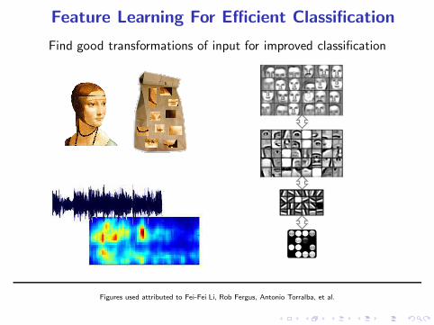
Feature Learning For Efficient Classification
Find good transformations of input for improved classification
Figures used attributed to Fei-Fei Li, Rob Fergus, Antonio Torralba, et al.
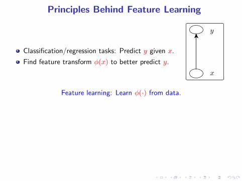
Principles Behind Feature Learning
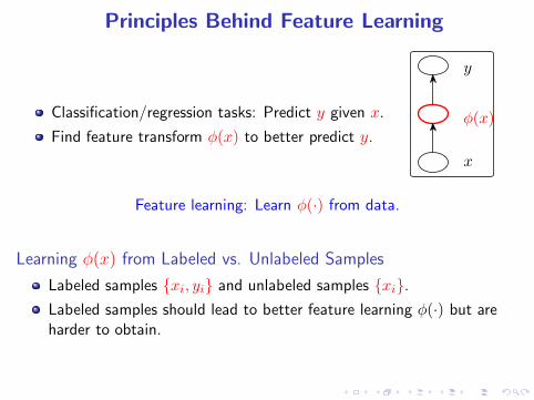
Classification/regression tasks: Predict y given x.
Find feature transform φ(x) to better predict y.
x
y
Feature learning: Learn φ(·) from data.
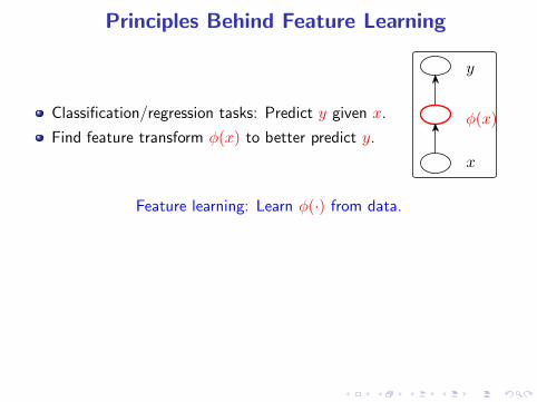
Principles Behind Feature Learning
Classification/regression tasks: Predict y given x.
Find feature transform φ(x) to better predict y.
x
φ(x)
y
Feature learning: Learn φ(·) from data.
Principles Behind Feature Learning
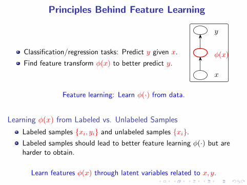
Classification/regression tasks: Predict y given x.
Find feature transform φ(x) to better predict y.
x
φ(x)
y
Feature learning: Learn φ(·) from data.
Learning φ(x) from Labeled vs. Unlabeled Samples
Labeled samples {xi, yi} and unlabeled samples {xi}.
Labeled samples should lead to better feature learning φ(·) but areharder to obtain.
Principles Behind Feature Learning
Classification/regression tasks: Predict y given x.
Find feature transform φ(x) to better predict y.
x
φ(x)
y
Feature learning: Learn φ(·) from data.
Learning φ(x) from Labeled vs. Unlabeled Samples
Labeled samples {xi, yi} and unlabeled samples {xi}.
Labeled samples should lead to better feature learning φ(·) but areharder to obtain.
Learn features φ(x) through latent variables related to x, y.
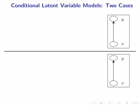
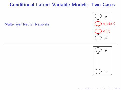
Conditional Latent Variable Models: Two Cases
x
y
x
y
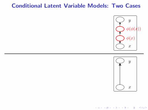
Conditional Latent Variable Models: Two Cases
x
φ(x)
φ(φ(x))
y
x
y
Conditional Latent Variable Models: Two Cases
Multi-layer Neural Networks
x
φ(x)
φ(φ(x))
y
x
y
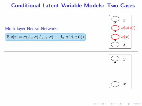
Conditional Latent Variable Models: Two Cases
Multi-layer Neural Networks
E[y|x] = σ(Ad σ(Ad−1 σ(· · ·A2 σ(A1x))))
x
φ(x)
φ(φ(x))
y
x
y
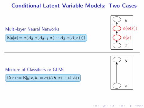
Conditional Latent Variable Models: Two Cases
Multi-layer Neural Networks
E[y|x] = σ(Ad σ(Ad−1 σ(· · ·A2 σ(A1x))))
x
φ(x)
φ(φ(x))
y
Mixture of Classifiers or GLMs
G(x) := E[y|x, h] = σ(〈Uh, x〉 + 〈b, h〉)
x
y
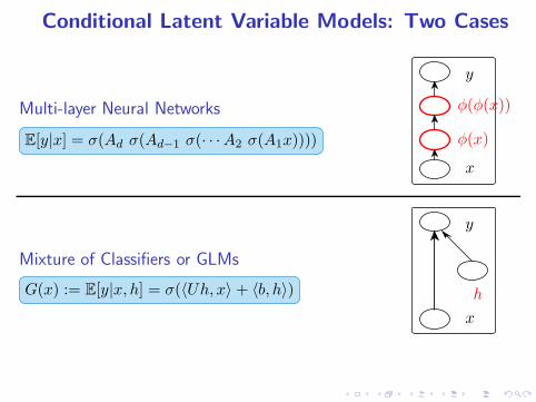
Conditional Latent Variable Models: Two Cases
Multi-layer Neural Networks
E[y|x] = σ(Ad σ(Ad−1 σ(· · ·A2 σ(A1x))))
x
φ(x)
φ(φ(x))
y
Mixture of Classifiers or GLMs
G(x) := E[y|x, h] = σ(〈Uh, x〉 + 〈b, h〉)
x
h
y
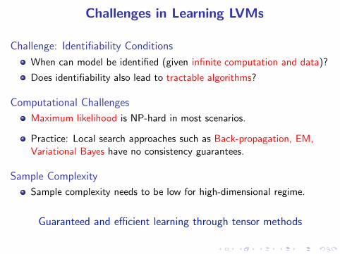
Challenges in Learning LVMs
Challenge: Identifiability Conditions
When can model be identified (given infinite computation and data)?
Does identifiability also lead to tractable algorithms?
Computational Challenges
Maximum likelihood is NP-hard in most scenarios.
Practice: Local search approaches such as Back-propagation, EM,Variational Bayes have no consistency guarantees.
Sample Complexity
Sample complexity needs to be low for high-dimensional regime.
Guaranteed and efficient learning through tensor methods
Outline
1 Introduction
2 Spectral and Tensor Methods
3 Generative Models for Feature Learning
4 Proposed Framework
5 Conclusion
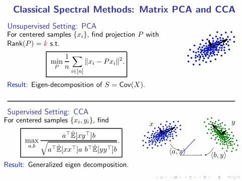
Classical Spectral Methods: Matrix PCA and CCA
Unsupervised Setting: PCAFor centered samples {xi}, find projection P withRank(P ) = k s.t.
minP
1
n
∑
i∈[n]
‖xi − Pxi‖2.
Result: Eigen-decomposition of S = Cov(X).
Supervised Setting: CCAFor centered samples {xi, yi}, find
maxa,b
a⊤E[xy⊤]b√
a⊤E[xx⊤]a b⊤E[yy⊤]b.
Result: Generalized eigen decomposition.
x y
〈a, x〉〈b, y〉
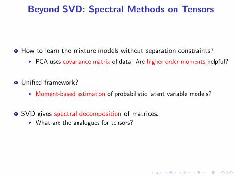
Beyond SVD: Spectral Methods on Tensors
How to learn the mixture models without separation constraints?
◮ PCA uses covariance matrix of data. Are higher order moments helpful?
Unified framework?
◮ Moment-based estimation of probabilistic latent variable models?
SVD gives spectral decomposition of matrices.◮ What are the analogues for tensors?
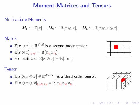
Moment Matrices and Tensors
Multivariate Moments
M1 := E[x], M2 := E[x⊗ x], M3 := E[x⊗ x⊗ x].
Matrix
E[x⊗ x] ∈ Rd×d is a second order tensor.
E[x⊗ x]i1,i2 = E[xi1xi2 ].
For matrices: E[x⊗ x] = E[xx⊤].
Tensor
E[x⊗ x⊗ x] ∈ Rd×d×d is a third order tensor.
E[x⊗ x⊗ x]i1,i2,i3 = E[xi1xi2xi3 ].
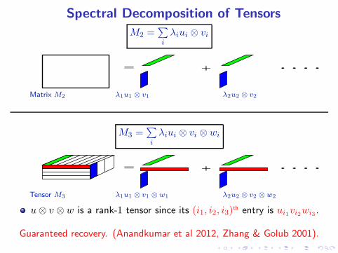
Spectral Decomposition of Tensors
M2 =∑
i
λiui ⊗ vi
= + ....
Matrix M2 λ1u1 ⊗ v1 λ2u2 ⊗ v2
M3 =∑
i
λiui ⊗ vi ⊗ wi
= + ....
Tensor M3 λ1u1 ⊗ v1 ⊗ w1 λ2u2 ⊗ v2 ⊗ w2
u⊗ v ⊗ w is a rank-1 tensor since its (i1, i2, i3)th entry is ui1vi2wi3 .
Guaranteed recovery. (Anandkumar et al 2012, Zhang & Golub 2001).
Moment Tensors for Conditional Models
Multivariate Moments: Many possibilities...
E[x⊗ y],E[x⊗ x⊗ y],E[φ(x)⊗ y] . . . .
Feature Transformations of the Input: x 7→ φ(x)
How to exploit them?
Are moments E[φ(x)⊗ y] useful?
If φ(x) is a matrix/tensor, we have matrix/tensor moments.
Can carry out spectral decomposition of the moments.
Construct φ(x) based on input distribution?
Outline
1 Introduction
2 Spectral and Tensor Methods
3 Generative Models for Feature Learning
4 Proposed Framework
5 Conclusion
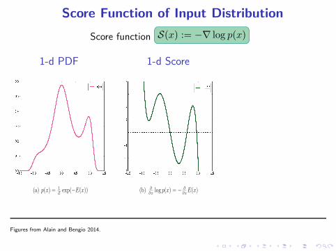
Score Function of Input Distribution
Score function S(x) := −∇ log p(x)
1-d PDF
(a) p(x) = 1
Zexp(−E(x))
1-d Score
(b) ∂
∂xlog p(x) = − ∂
∂xE(x)
Figures from Alain and Bengio 2014.
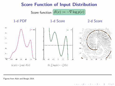
Score Function of Input Distribution
Score function S(x) := −∇ log p(x)
1-d PDF
(a) p(x) = 1
Zexp(−E(x))
1-d Score
(b) ∂
∂xlog p(x) = − ∂
∂xE(x)
2-d Score
Figures from Alain and Bengio 2014.

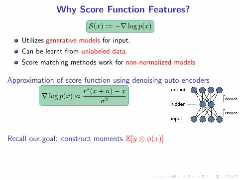
Why Score Function Features?
S(x) := −∇ log p(x)
Utilizes generative models for input.
Can be learnt from unlabeled data.
Score matching methods work for non-normalized models.
Why Score Function Features?
S(x) := −∇ log p(x)
Utilizes generative models for input.
Can be learnt from unlabeled data.
Score matching methods work for non-normalized models.
Approximation of score function using denoising auto-encoders
∇ log p(x) ≈r∗(x+ n)− x
σ2
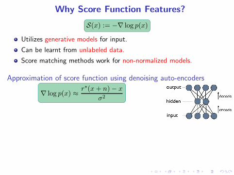
Why Score Function Features?
S(x) := −∇ log p(x)
Utilizes generative models for input.
Can be learnt from unlabeled data.
Score matching methods work for non-normalized models.
Approximation of score function using denoising auto-encoders
∇ log p(x) ≈r∗(x+ n)− x
σ2
Recall our goal: construct moments E[y ⊗ φ(x)]
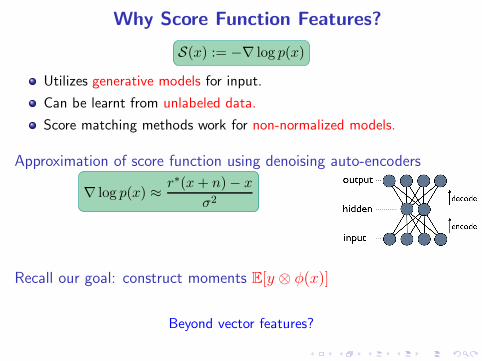
Beyond vector features?

Matrix and Tensor-valued Features
Higher order score functions
Sm(x) := (−1)m∇(m)p(x)
p(x)
Can be a matrix or a tensor instead of a vector.
Can be used to construct matrix and tensor moments E[y ⊗ φ(x)].
Outline
1 Introduction
2 Spectral and Tensor Methods
3 Generative Models for Feature Learning
4 Proposed Framework
5 Conclusion
Operations on Score Function Features
Form the cross-moments: E [y ⊗ Sm(x)].
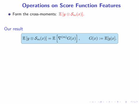
Operations on Score Function Features
Form the cross-moments: E [y ⊗ Sm(x)].
Our result
E [y ⊗ Sm(x)] = E
[
∇(m)G(x)]
, G(x) := E[y|x].
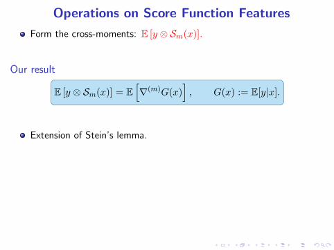
Operations on Score Function Features
Form the cross-moments: E [y ⊗ Sm(x)].
Our result
E [y ⊗ Sm(x)] = E
[
∇(m)G(x)]
, G(x) := E[y|x].
Extension of Stein’s lemma.
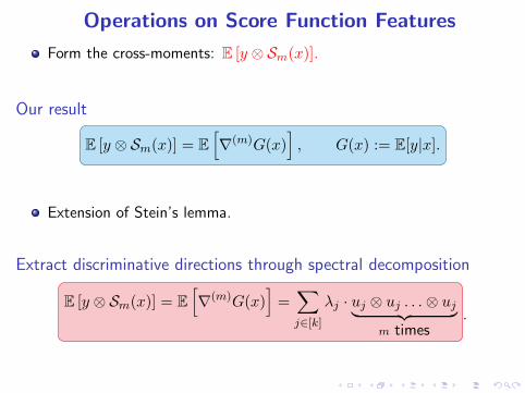
Operations on Score Function Features
Form the cross-moments: E [y ⊗ Sm(x)].
Our result
E [y ⊗ Sm(x)] = E
[
∇(m)G(x)]
, G(x) := E[y|x].
Extension of Stein’s lemma.
Extract discriminative directions through spectral decomposition
E [y ⊗ Sm(x)] = E
[
∇(m)G(x)]
=∑
j∈[k]
λj · uj ⊗ uj . . .⊗ uj︸ ︷︷ ︸
m times.
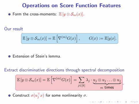
Construct σ(u⊤j x) for some nonlinearity σ.
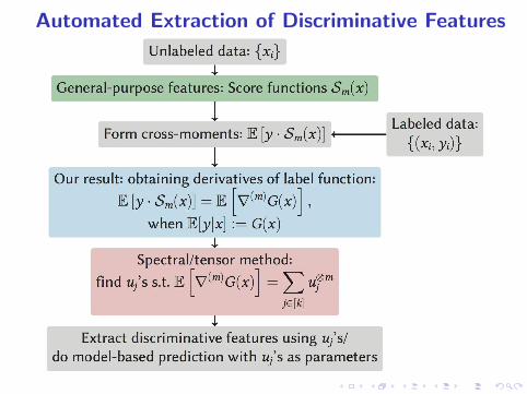
Automated Extraction of Discriminative Features
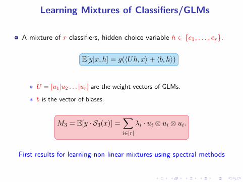
Learning Mixtures of Classifiers/GLMs
A mixture of r classifiers, hidden choice variable h ∈ {e1, . . . , er}.
E[y|x, h] = g(〈Uh, x〉 + 〈b, h〉)
∗ U = [u1|u2 . . . |ur] are the weight vectors of GLMs.
∗ b is the vector of biases.
M3 = E[y · S3(x)] =∑
i∈[r]
λi · ui ⊗ ui ⊗ ui.
First results for learning non-linear mixtures using spectral methods
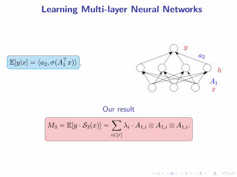
Learning Multi-layer Neural Networks
E[y|x] = 〈a2, σ(A⊤1 x)〉 .
A1
a2
x
h
y
Our result
M3 = E[y · S3(x)] =∑
i∈[r]
λi · A1,i ⊗A1,i ⊗A1,i.
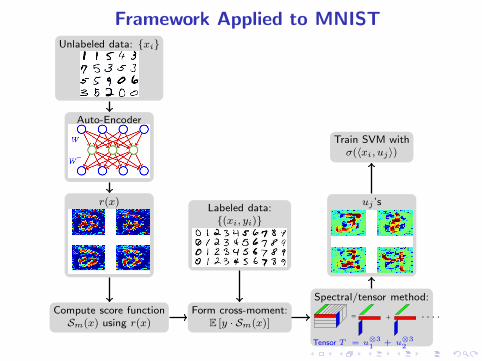
Framework Applied to MNISTUnlabeled data: {xi}
Auto-Encoder
Train SVM withσ(〈xi, uj〉)
r(x)Labeled data:{(xi, yi)}
uj ’s
Compute score functionSm(x) using r(x)
Form cross-moment:E [y · Sm(x)]
Spectral/tensor method:
= + ....
Tensor T = u⊗3
1+ u
⊗3
2
Outline
1 Introduction
2 Spectral and Tensor Methods
3 Generative Models for Feature Learning
4 Proposed Framework
5 Conclusion
Conclusion: Learning Conditional Models using
Tensor Methods
Tensor Decomposition
Efficient sample and computational complexities
Better performance compared to EM, Variational Bayes etc.
Scalable and embarrassingly parallel: handle large datasets.
Score function features
Score function features crucial for learning conditional models.
Related: Guaranteed Non-convex Methods
Overcomplete Dictionary Learning/Sparse Coding: Decompose datainto a sparse combination of unknown dictionary elements.
Non-convex robust PCA: Same guarantees as convex relaxationmethods, lower computational complexity. Extensions to tensorsetting.

Co-authors and Resources
Majid Janzamin Hanie Sedghi
Niranjan UN
Papers available at http://newport.eecs.uci.edu/anandkumar/
Top Related