Tensor Methods for Feature Learning
41
Tensor Methods for Feature Learning Anima Anandkumar U.C. Irvine
Transcript of Tensor Methods for Feature Learning
Tensor Methods for Feature Learning
Anima Anandkumar
U.C. Irvine
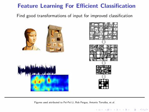
Feature Learning For Efficient Classification
Find good transformations of input for improved classification
Figures used attributed to Fei-Fei Li, Rob Fergus, Antonio Torralba, et al.
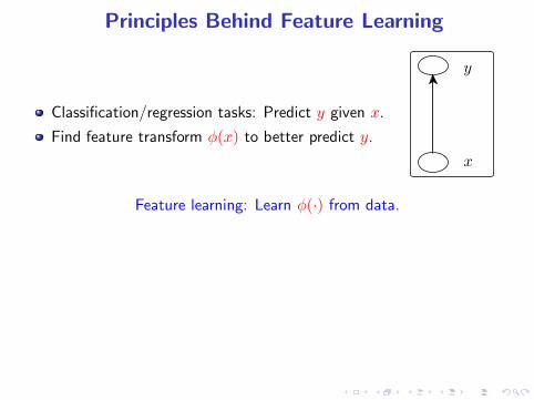
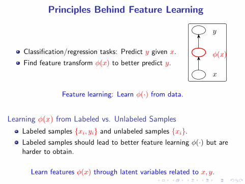
Principles Behind Feature Learning
Classification/regression tasks: Predict y given x.
Find feature transform φ(x) to better predict y.
x
y
Feature learning: Learn φ(·) from data.
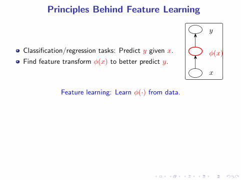
Principles Behind Feature Learning
Classification/regression tasks: Predict y given x.
Find feature transform φ(x) to better predict y.
x
φ(x)
y
Feature learning: Learn φ(·) from data.
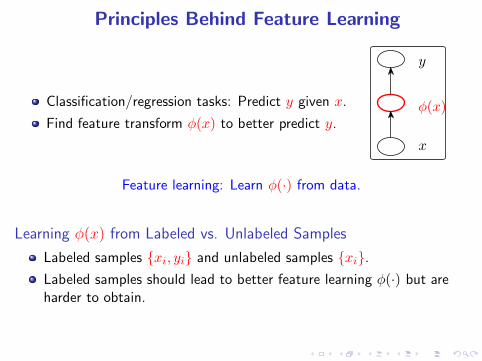
Principles Behind Feature Learning
Classification/regression tasks: Predict y given x.
Find feature transform φ(x) to better predict y.
x
φ(x)
y
Feature learning: Learn φ(·) from data.
Learning φ(x) from Labeled vs. Unlabeled Samples
Labeled samples {xi, yi} and unlabeled samples {xi}.
Labeled samples should lead to better feature learning φ(·) but areharder to obtain.
Learn features φ(x) through latent variables related to x, y.
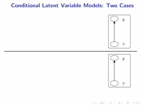
Conditional Latent Variable Models: Two Cases
x
y
x
y
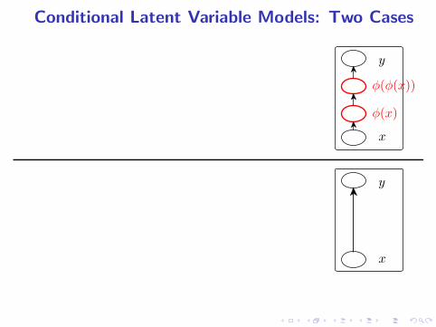
Conditional Latent Variable Models: Two Cases
x
φ(x)
φ(φ(x))
y
x
y
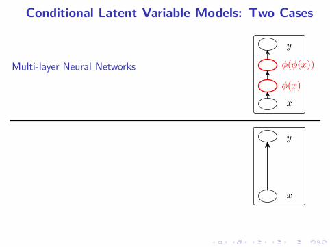
Conditional Latent Variable Models: Two Cases
Multi-layer Neural Networks
x
φ(x)
φ(φ(x))
y
x
y
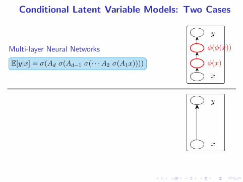
Conditional Latent Variable Models: Two Cases
Multi-layer Neural Networks
E[y|x] = σ(Ad σ(Ad−1 σ(· · ·A2 σ(A1x))))
x
φ(x)
φ(φ(x))
y
x
y
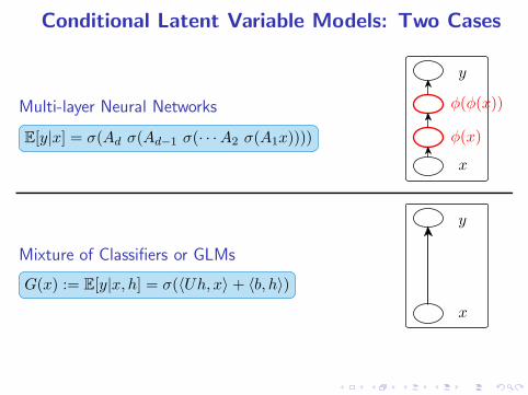
Conditional Latent Variable Models: Two Cases
Multi-layer Neural Networks
E[y|x] = σ(Ad σ(Ad−1 σ(· · ·A2 σ(A1x))))
x
φ(x)
φ(φ(x))
y
Mixture of Classifiers or GLMs
G(x) := E[y|x, h] = σ(〈Uh, x〉 + 〈b, h〉)
x
y
Conditional Latent Variable Models: Two Cases
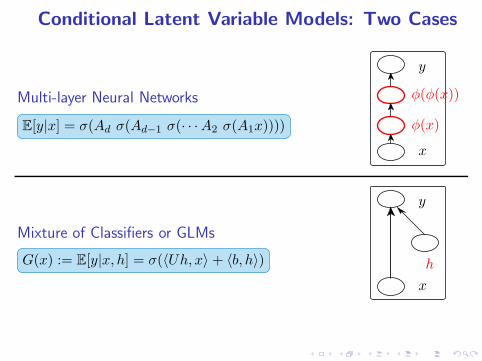
Multi-layer Neural Networks
E[y|x] = σ(Ad σ(Ad−1 σ(· · ·A2 σ(A1x))))
x
φ(x)
φ(φ(x))
y
Mixture of Classifiers or GLMs
G(x) := E[y|x, h] = σ(〈Uh, x〉 + 〈b, h〉)
x
h
y
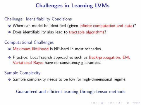
Challenges in Learning LVMs
Challenge: Identifiability Conditions
When can model be identified (given infinite computation and data)?
Does identifiability also lead to tractable algorithms?
Computational Challenges
Maximum likelihood is NP-hard in most scenarios.
Practice: Local search approaches such as Back-propagation, EM,Variational Bayes have no consistency guarantees.
Sample Complexity
Sample complexity needs to be low for high-dimensional regime.
Guaranteed and efficient learning through tensor methods
Outline
1 Introduction
2 Spectral and Tensor Methods
3 Generative Models for Feature Learning
4 Proposed Framework
5 Conclusion
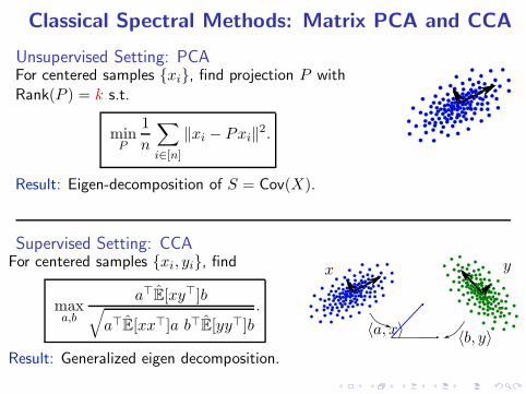
Classical Spectral Methods: Matrix PCA and CCA
Unsupervised Setting: PCAFor centered samples {xi}, find projection P withRank(P ) = k s.t.
minP
1
n
∑
i∈[n]
‖xi − Pxi‖2.
Result: Eigen-decomposition of S = Cov(X).
Supervised Setting: CCAFor centered samples {xi, yi}, find
maxa,b
a⊤E[xy⊤]b√
a⊤E[xx⊤]a b⊤E[yy⊤]b.
Result: Generalized eigen decomposition.
x y
〈a, x〉〈b, y〉
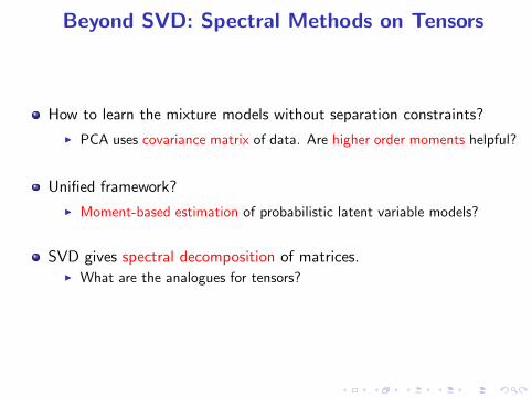
Beyond SVD: Spectral Methods on Tensors
How to learn the mixture models without separation constraints?
◮ PCA uses covariance matrix of data. Are higher order moments helpful?
Unified framework?
◮ Moment-based estimation of probabilistic latent variable models?
SVD gives spectral decomposition of matrices.◮ What are the analogues for tensors?
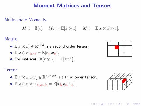
Moment Matrices and Tensors
Multivariate Moments
M1 := E[x], M2 := E[x⊗ x], M3 := E[x⊗ x⊗ x].
Matrix
E[x⊗ x] ∈ Rd×d is a second order tensor.
E[x⊗ x]i1,i2 = E[xi1xi2 ].
For matrices: E[x⊗ x] = E[xx⊤].
Tensor
E[x⊗ x⊗ x] ∈ Rd×d×d is a third order tensor.
E[x⊗ x⊗ x]i1,i2,i3 = E[xi1xi2xi3 ].
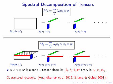
Spectral Decomposition of Tensors
M2 =∑
i
λiui ⊗ vi
= + ....
Matrix M2 λ1u1 ⊗ v1 λ2u2 ⊗ v2
M3 =∑
i
λiui ⊗ vi ⊗ wi
= + ....
Tensor M3 λ1u1 ⊗ v1 ⊗ w1 λ2u2 ⊗ v2 ⊗ w2
u⊗ v ⊗ w is a rank-1 tensor since its (i1, i2, i3)th entry is ui1vi2wi3 .
Guaranteed recovery. (Anandkumar et al 2012, Zhang & Golub 2001).
Moment Tensors for Conditional Models
Multivariate Moments: Many possibilities...
E[x⊗ y],E[x⊗ x⊗ y],E[φ(x)⊗ y] . . . .
Feature Transformations of the Input: x 7→ φ(x)
How to exploit them?
Are moments E[φ(x)⊗ y] useful?
If φ(x) is a matrix/tensor, we have matrix/tensor moments.
Can carry out spectral decomposition of the moments.
Construct φ(x) based on input distribution?
Outline
1 Introduction
2 Spectral and Tensor Methods
3 Generative Models for Feature Learning
4 Proposed Framework
5 Conclusion
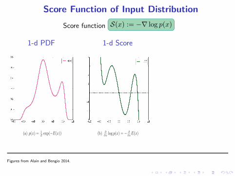
Score Function of Input Distribution
Score function S(x) := −∇ log p(x)
1-d PDF
(a) p(x) = 1
Zexp(−E(x))
1-d Score
(b) ∂
∂xlog p(x) = − ∂
∂xE(x)
Figures from Alain and Bengio 2014.
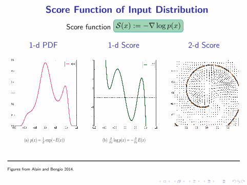
Score Function of Input Distribution
Score function S(x) := −∇ log p(x)
1-d PDF
(a) p(x) = 1
Zexp(−E(x))
1-d Score
(b) ∂
∂xlog p(x) = − ∂
∂xE(x)
2-d Score
Figures from Alain and Bengio 2014.

Why Score Function Features?
S(x) := −∇ log p(x)
Utilizes generative models for input.
Can be learnt from unlabeled data.
Score matching methods work for non-normalized models.
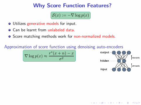
Why Score Function Features?
S(x) := −∇ log p(x)
Utilizes generative models for input.
Can be learnt from unlabeled data.
Score matching methods work for non-normalized models.
Approximation of score function using denoising auto-encoders
∇ log p(x) ≈r∗(x+ n)− x
σ2
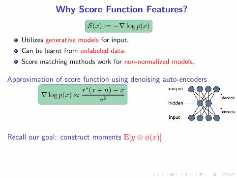
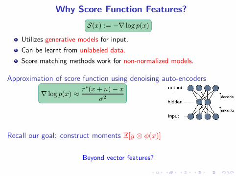
Why Score Function Features?
S(x) := −∇ log p(x)
Utilizes generative models for input.
Can be learnt from unlabeled data.
Score matching methods work for non-normalized models.
Approximation of score function using denoising auto-encoders
∇ log p(x) ≈r∗(x+ n)− x
σ2
Recall our goal: construct moments E[y ⊗ φ(x)]
Beyond vector features?

Matrix and Tensor-valued Features
Higher order score functions
Sm(x) := (−1)m∇(m)p(x)
p(x)
Can be a matrix or a tensor instead of a vector.
Can be used to construct matrix and tensor moments E[y ⊗ φ(x)].
Outline
1 Introduction
2 Spectral and Tensor Methods
3 Generative Models for Feature Learning
4 Proposed Framework
5 Conclusion
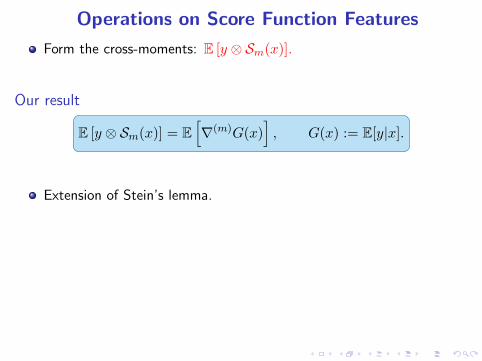
Operations on Score Function Features
Form the cross-moments: E [y ⊗ Sm(x)].
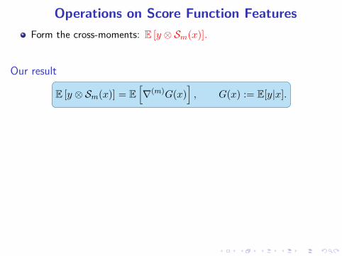
Operations on Score Function Features
Form the cross-moments: E [y ⊗ Sm(x)].
Our result
E [y ⊗ Sm(x)] = E
[
∇(m)G(x)]
, G(x) := E[y|x].
Operations on Score Function Features
Form the cross-moments: E [y ⊗ Sm(x)].
Our result
E [y ⊗ Sm(x)] = E
[
∇(m)G(x)]
, G(x) := E[y|x].
Extension of Stein’s lemma.
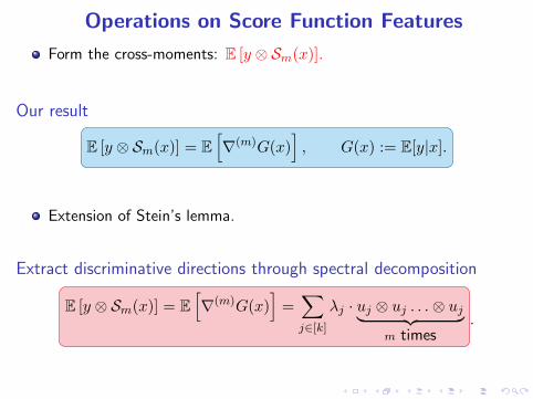
Operations on Score Function Features
Form the cross-moments: E [y ⊗ Sm(x)].
Our result
E [y ⊗ Sm(x)] = E
[
∇(m)G(x)]
, G(x) := E[y|x].
Extension of Stein’s lemma.
Extract discriminative directions through spectral decomposition
E [y ⊗ Sm(x)] = E
[
∇(m)G(x)]
=∑
j∈[k]
λj · uj ⊗ uj . . .⊗ uj︸ ︷︷ ︸
m times.
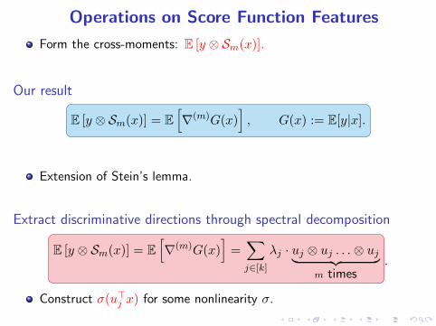
Construct σ(u⊤j x) for some nonlinearity σ.
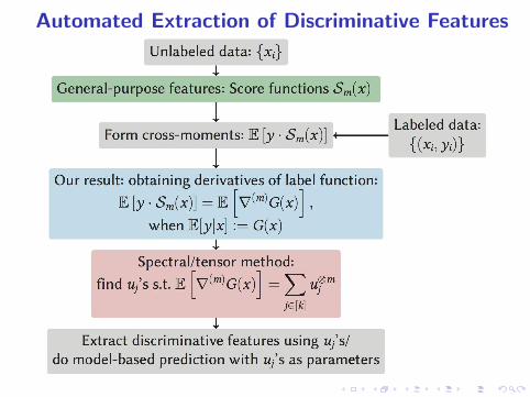
Automated Extraction of Discriminative Features
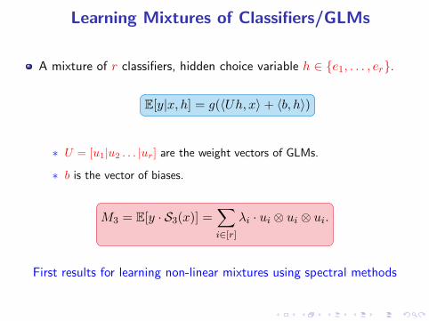
Learning Mixtures of Classifiers/GLMs
A mixture of r classifiers, hidden choice variable h ∈ {e1, . . . , er}.
E[y|x, h] = g(〈Uh, x〉 + 〈b, h〉)
∗ U = [u1|u2 . . . |ur] are the weight vectors of GLMs.
∗ b is the vector of biases.
M3 = E[y · S3(x)] =∑
i∈[r]
λi · ui ⊗ ui ⊗ ui.
First results for learning non-linear mixtures using spectral methods
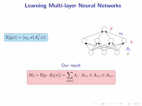
Learning Multi-layer Neural Networks
E[y|x] = 〈a2, σ(A⊤1 x)〉 .
A1
a2
x
h
y
Our result
M3 = E[y · S3(x)] =∑
i∈[r]
λi · A1,i ⊗A1,i ⊗A1,i.
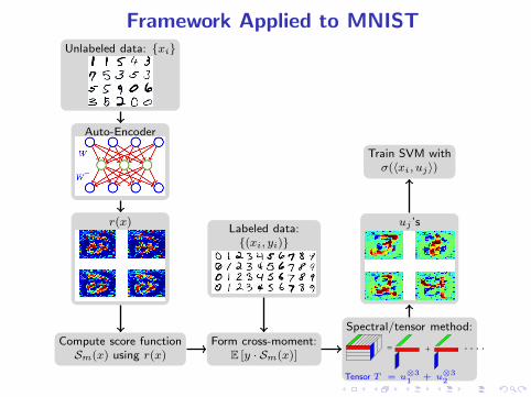
Framework Applied to MNISTUnlabeled data: {xi}
Auto-Encoder
Train SVM withσ(〈xi, uj〉)
r(x)Labeled data:{(xi, yi)}
uj ’s
Compute score functionSm(x) using r(x)
Form cross-moment:E [y · Sm(x)]
Spectral/tensor method:
= + ....
Tensor T = u⊗3
1+ u
⊗3
2
Outline
1 Introduction
2 Spectral and Tensor Methods
3 Generative Models for Feature Learning
4 Proposed Framework
5 Conclusion
Conclusion: Learning Conditional Models using
Tensor Methods
Tensor Decomposition
Efficient sample and computational complexities
Better performance compared to EM, Variational Bayes etc.
Scalable and embarrassingly parallel: handle large datasets.
Score function features
Score function features crucial for learning conditional models.
Related: Guaranteed Non-convex Methods
Overcomplete Dictionary Learning/Sparse Coding: Decompose datainto a sparse combination of unknown dictionary elements.
Non-convex robust PCA: Same guarantees as convex relaxationmethods, lower computational complexity. Extensions to tensorsetting.

Co-authors and Resources
Majid Janzamin Hanie Sedghi
Niranjan UN
Papers available at http://newport.eecs.uci.edu/anandkumar/