


γλώσσες
Σελίδες
Νομικός

SAXS/SANS data processing and overall parameters
Petr V. Konarev
European Molecular Biology Laboratory,Hamburg Outstation
BioSAXS group
EMBO Global Exchange Lecture Course 30 November 2012 Hyderabad India

Detector
k1
Scattering vector s=k1-k,s=4π sinθ/λ
Radiation sources:
X-ray generator (λ = 0.1 - 0.2 nm)Synchrotron (λ = 0.03 - 0.35 nm)Thermal neutrons (λ = 0.2 - 1 nm)
Monochromatic beam
Sample
2θWave vector k, k=2π/λ
Small-angle scattering: experiment
s=4π sinθ/λ, nm-10 1 2 3
Log (Intensity)
-1
0
1
2
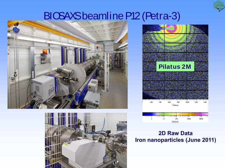
BIOSAXS beamline P12 (Petra-3)
Pilatus 2M
2D Raw Data Iron nanoparticles (June 2011)

PILATUS Pixel X-ray Detector at P12PILATUS 2M (24*100K modules) Active area 250*290 mm2 , pixel size: 172μm Readout time: 3.6ms, framing rate: 50Hz
Silver behenate Axis calibration standard
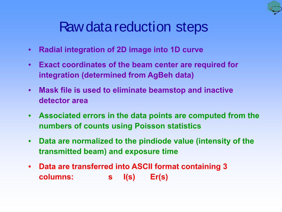
Raw data reduction steps
• Radial integration of 2D image into 1D curve
• Exact coordinates of the beam center are required for integration (determined from AgBeh data)
• Mask file is used to eliminate beamstop and inactive detector area
• Associated errors in the data points are computed from the numbers of counts using Poisson statistics
• Data are normalized to the pindiode value (intensity of the transmitted beam) and exposure time
• Data are transferred into ASCII format containing 3 columns: s I(s) Er(s)
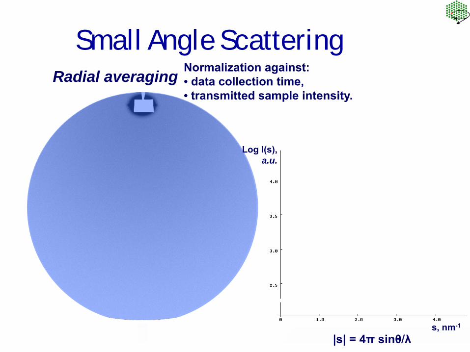
Normalization against:• data collection time,• transmitted sample intensity.
Log I(s),a.u.
s, nm-1
|s| = 4π sinθ/λ
Small Angle ScatteringRadial averaging
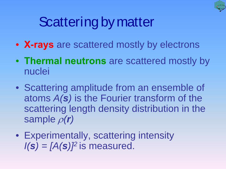
Scattering by matter
• X-rays are scattered mostly by electrons
• Thermal neutrons are scattered mostly by nuclei
• Scattering amplitude from an ensemble of atoms A(s) is the Fourier transform of the scattering length density distribution in the sample ρ(r)
• Experimentally, scattering intensity I(s) = [A(s)]2 is measured.
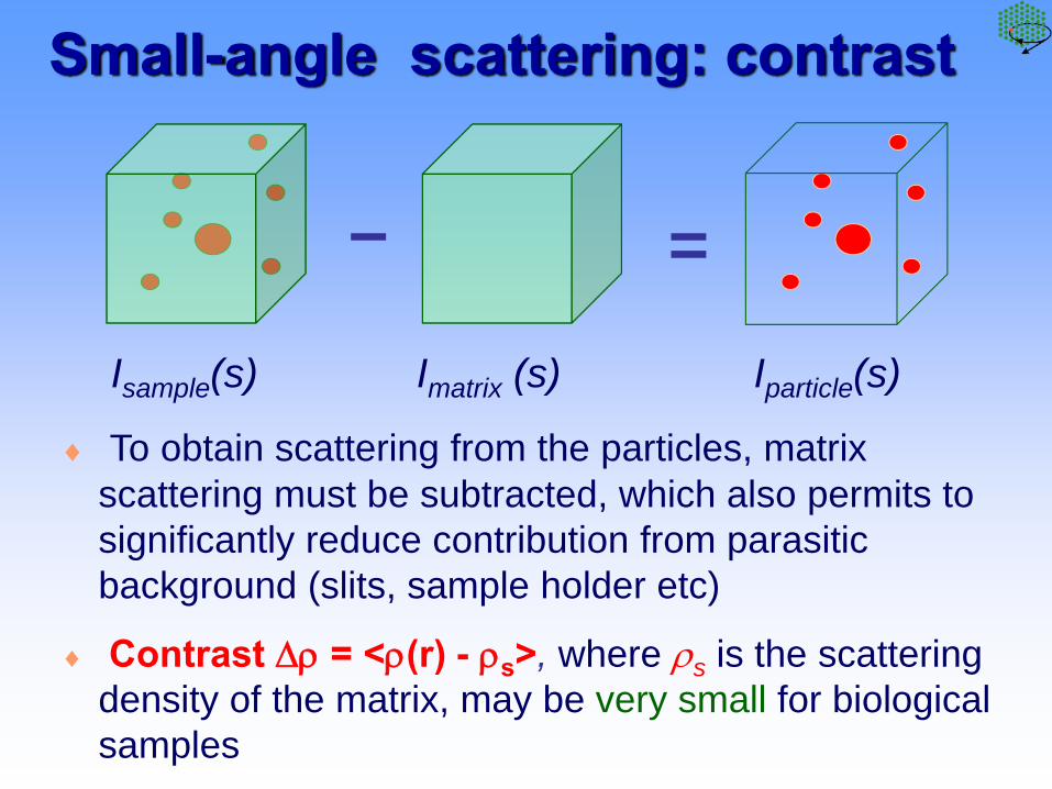
Small-angle scattering: contrast
Isample(s) Imatrix (s) Iparticle(s)
♦ To obtain scattering from the particles, matrix scattering must be subtracted, which also permits to significantly reduce contribution from parasitic background (slits, sample holder etc)
♦ Contrast Δρ = <ρ(r) - ρs>, where ρs is the scattering density of the matrix, may be very small for biological samples

X-rays neutrons
• X-rays: scattering factor increases with atomic number, no difference between H and D
• Neutrons: scattering factor is irregular, may be negative, huge difference between H and D
Element H D C N O P S Au At. Weight 1 2 12 14 16 30 32 197 N electrons 1 1 6 7 8 15 16 79 bX,10-12 cm 0.282 0.282 1.69 1.97 2.16 3.23 4.51 22.3 bN,10-12 cm -0.374 0.667 0.665 0.940 0.580 0.510 0.280 0.760
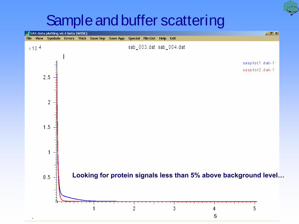
Sample and buffer scattering
Looking for protein signals less than 5% above background level…

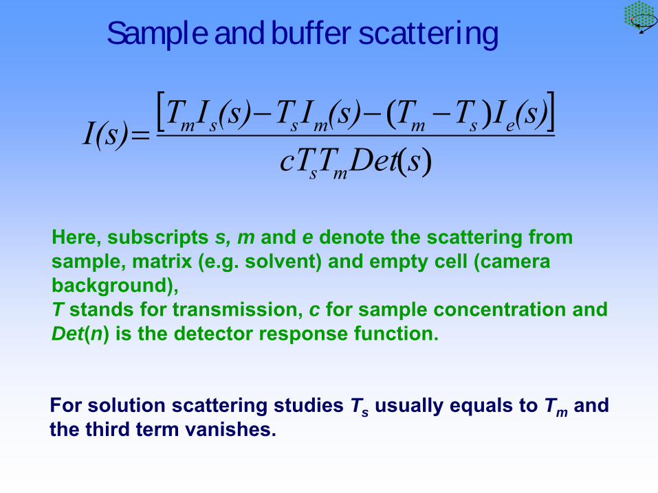
Sample and buffer scattering
[ ])(
)(sDetTcT
(s)ITT(s)IT(s)ITI(s)ms
esmmssm −−−=
Here, subscripts s, m and e denote the scattering from sample, matrix (e.g. solvent) and empty cell (camera background),T stands for transmission, c for sample concentration and Det(n) is the detector response function.
For solution scattering studies Ts usually equals to Tm and the third term vanishes.
Sample and buffer scattering

s, nm -10 2 4 6 8
lg I
, re
lative
1
2
3
Scattering curve I(s)
Overall Parameters
Rg
Dmax
MMexp
Excluded Volume
Analysis of biological SAS data

Overall parameters
) sR)I(I(s) g22
31exp(0 −≅
Radius of gyration Rg (Guinier, 1939)
Maximum size Dmax: p(r)=0 for r> Dmax
Excluded particle volume (Porod, 1952)
∫∞
==0
22 )( I(0)/Q;2V dssIsQπ
Maximum size Dmax: p(r)=0 for r> Dmax

Program PRIMUS- graphical package for data manipulations and analysis
♦data manipulations (averaging, background subtraction, merging of data in different angular ranges, extrapolation to infinite dilution )
♦evaluation of radius of gyration and forward intensity (Guinier plot, module AUTORG), estimation of Porod volume
♦calculation of distance/size distribution function p(r)/V(r) (module GNOM)
♦data fitting using the parameters of simple geometrical bodies (ellipsoid, elliptic/hollow cylinder, rectangular prism) (module BODIES)
♦data analysis for polydisperse and interacting systems, mixtures and partially ordered systems (modules OLIGOMER, SVDPLOT, MIXTURE and PEAK)
P.V. Konarev, V.V. Volkov, A.V. Sokolova, M.H.J. Koch, D.I. Svergun J.Appl. Cryst. (2003) 36, 1277-1282

PRIMUS: graphical user interface

Data qualityRadiation damage
Log I(s), a.u.
s, nm-1
sample

Data qualityRadiation damage
s, nm-1
samplesame sample again
RADIATION DAMAGE!
Log I(s), a.u.

Low and High ConcentrationLog I(s)
s, nm-1
1 mg/ml10 mg/ml
Merging data
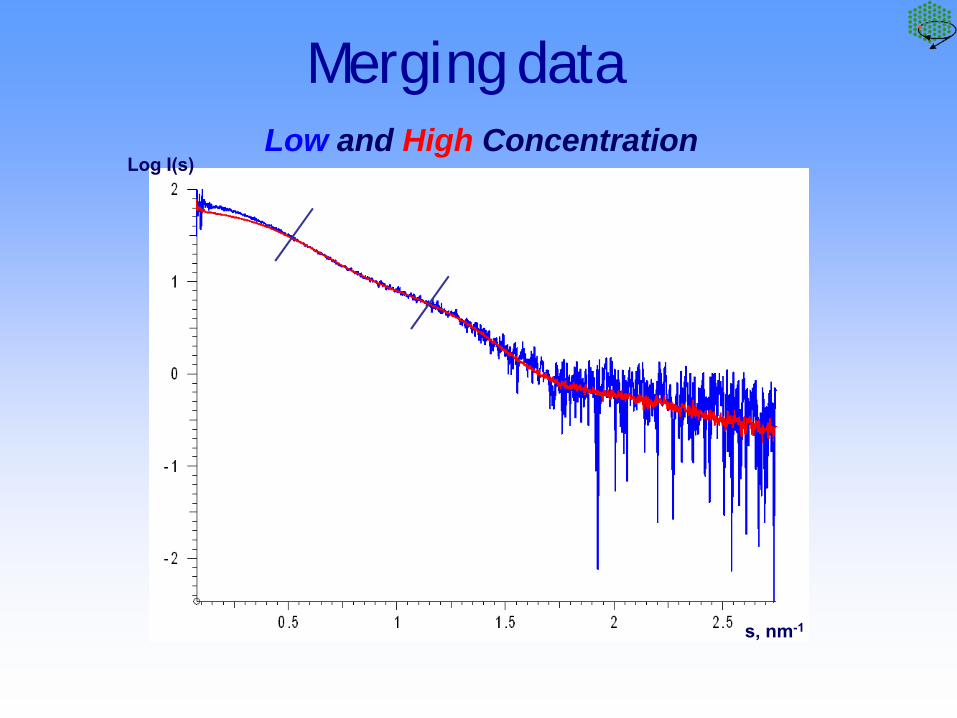
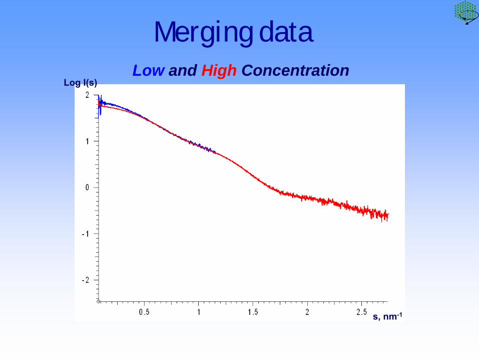
Low and High ConcentrationLog I(s)
s, nm-1
Merging data
Merging dataLow and High Concentration
Log I(s)
s, nm-1

Low and High ConcentrationLog I(s)
s, nm-1
Merging data
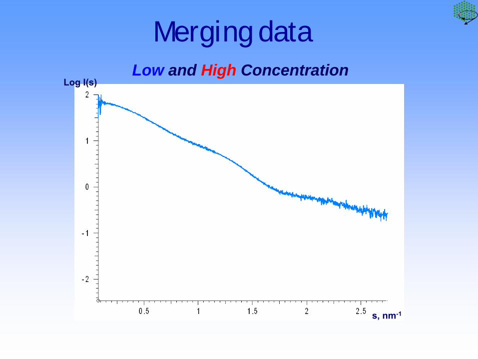
Low and High ConcentrationLog I(s)
s, nm-1
Merging data
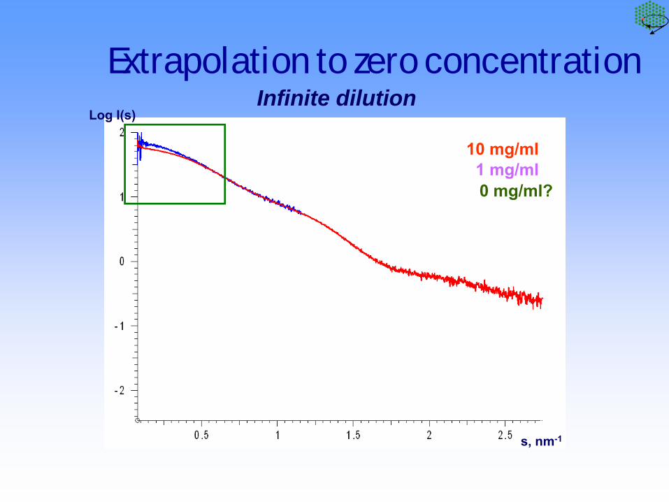
Extrapolation to zero concentrationInfinite dilution
Log I(s)
s, nm-1
10 mg/ml1 mg/ml0 mg/ml?

Shape and size
lysozyme
apoferritin
Log I(s)a.u.
s, nm-1
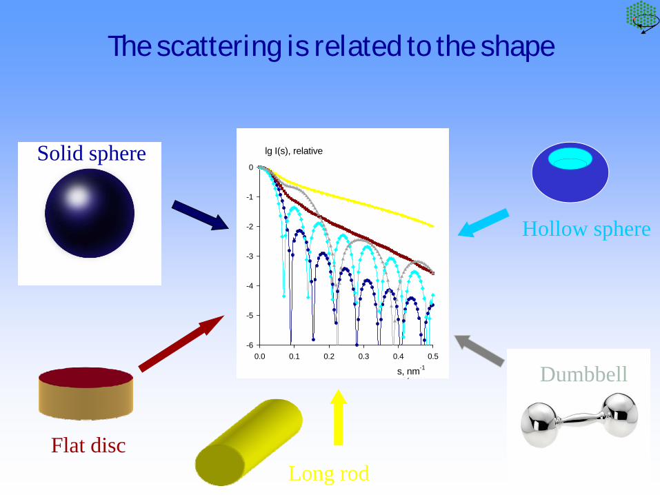
The scattering is related to the shape
s, nm-1
0.0 0.1 0.2 0.3 0.4 0.5
lg I(s), relative
-6
-5
-4
-3
-2
-1
0Solid sphere
Long rodFlat disc
Hollow sphere
Dumbbells, nm-1
0.0 0.1 0.2 0.3 0.4 0.5
lg I(s), relative
-6
-5
-4
-3
-2
-1
0
s, nm-1
0.0 0.1 0.2 0.3 0.4 0.5
lg I(s), relative
-6
-5
-4
-3
-2
-1
0
s, nm-1
0.0 0.1 0.2 0.3 0.4 0.5
lg I(s), relative
-6
-5
-4
-3
-2
-1
0
s, nm-1
0.0 0.1 0.2 0.3 0.4 0.5
lg I(s), relative
-6
-5
-4
-3
-2
-1
0
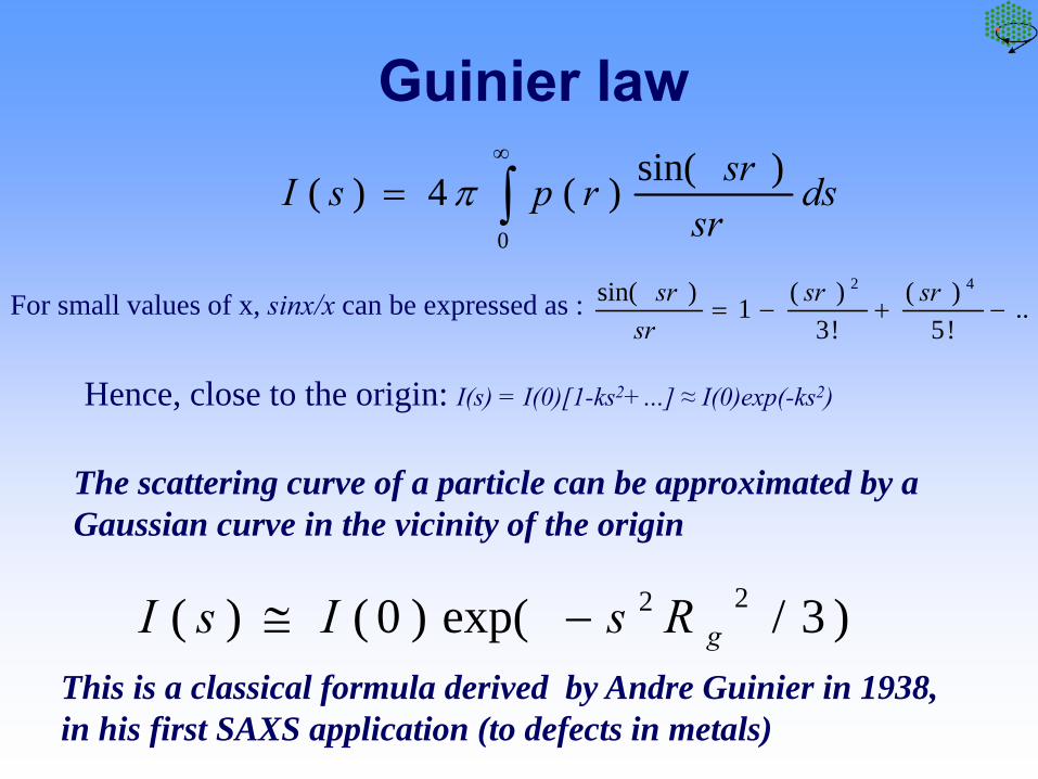
Guinier law
For small values of x, sinx/x can be expressed as :
Hence, close to the origin: I(s) = I(0)[1-ks2+…] ≈ I(0)exp(-ks2)
The scattering curve of a particle can be approximated by a Gaussian curve in the vicinity of the origin
∫∞
=0
)sin()(4)( dssr
srrpsI π
..!5)(
!3)(1)sin( 42
−+−=srsr
srsr
This is a classical formula derived by Andre Guinier in 1938, in his first SAXS application (to defects in metals)
)3/exp()0()( 22gRsIsI −≅

Radius of gyration
Radius of gyration :2
2( )
( )V
g
V
r dVR
dV
ρ
ρ
Δ=
Δ
∫∫r
r
r
r
r
r
Rg is the quadratic mean of distances to the center of mass weighted by the contrast of electron density.Rg is an index of non sphericity.For a given volume the smallest Rg is that of a sphere :
Ellipsoïd of revolution (a, b) Cylinder (D, H)
35gR R=
2 225g
a bR +=
2 2
8 12gD HR = +
idealmonodisperse
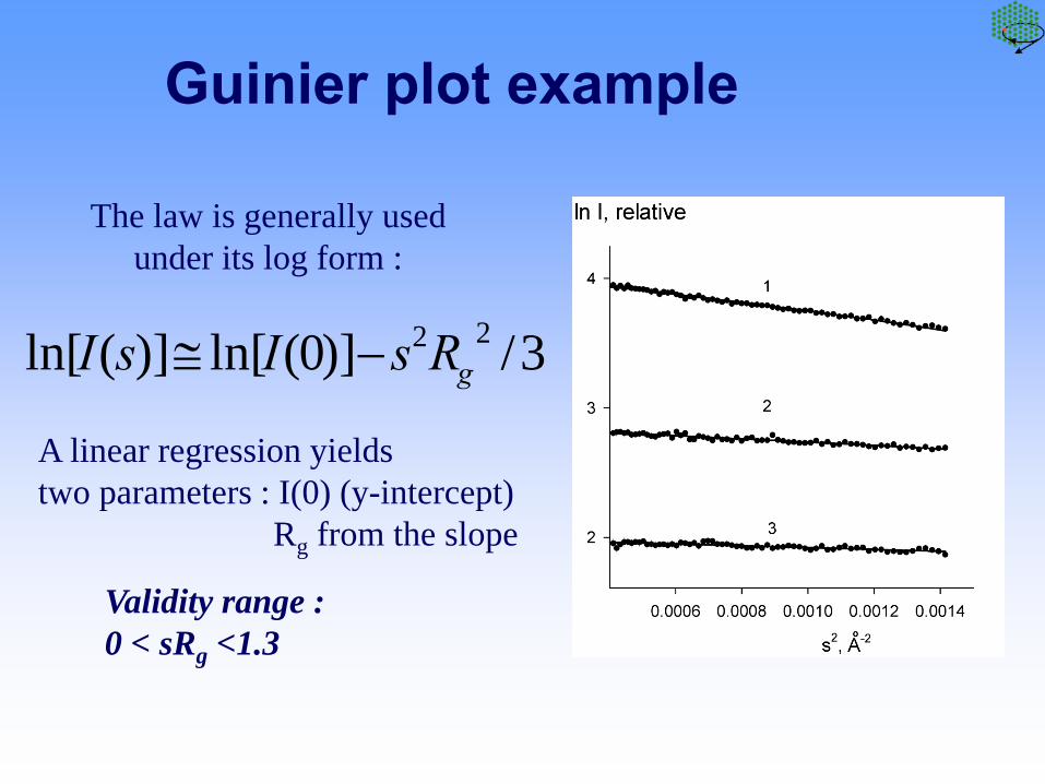
Guinier plot example
Validity range : 0 < sRg <1.3
The law is generally used under its log form :
A linear regression yields two parameters : I(0) (y-intercept)
Rg from the slope
3/)]0(ln[)](ln[ 22gRsIsI −≅

Guinier
PRIMUS: Guinier plot
Rg = 2.68 +- 1.11e-2
I0 = 271.07 +- 0.605
)3exp()0()( 22 RgsIsI ⋅−⋅=
Rg – radius of gyration
M≈MBSA*(I(0)/IBSA(0))

PRIMUS: AutoRG moduleAutoRg
Petoukhov, M.V., Konarev, P.V., Kikhney, A.G. & Svergun, D.I.
(2007) J. Appl. Cryst., 40, s223-s228.

In the case of very elongated particles, the radius of gyration of the cross-section can be derived using a similar representation, plotting this time sI(s) vs s2
Finally, in the case of a platelet, a thickness parameter is derived from a plot of s2I(s) vs s2 :
with T : thickness
Rods and platelets
)2/exp()( 22cRsssI −∝
)exp()( 222tRssIs −∝
12/TRt =
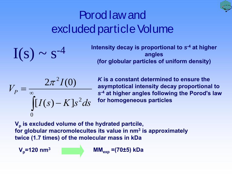
Porod law and excluded particle Volume
I(s) ~ s-4 Intensity decay is proportional to s-4 at higher angles
(for globular particles of uniform density)
∫∞
−=
0
2
2
])([
)0(2
dssKsI
IVPπ K is a constant determined to ensure the
asymptotical intensity decay proportional to s-4 at higher angles following the Porod's law for homogeneous particles
Vp is excluded volume of the hydrated partcile,for globular macromolecultes its value in nm3 is approximately twice (1.7 times) of the molecular mass in kDa
Vp=120 nm3 MMexp =(70±5) kDa
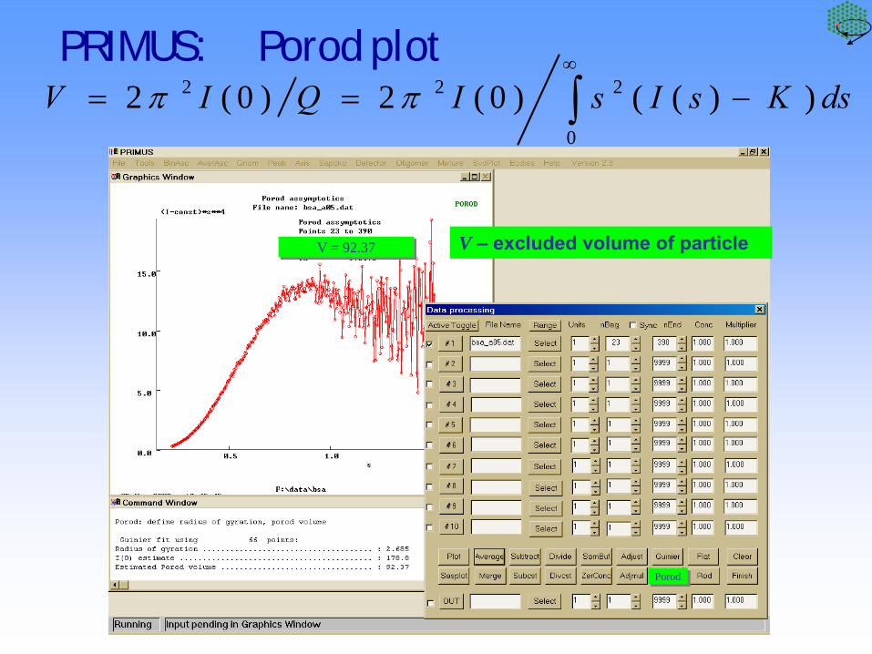
PRIMUS: Porod plot
Porod
))(()0(2)0(20
222 ∫∞
−== dsKsIsIQIV ππ
V – excluded volume of particleV = 92.37

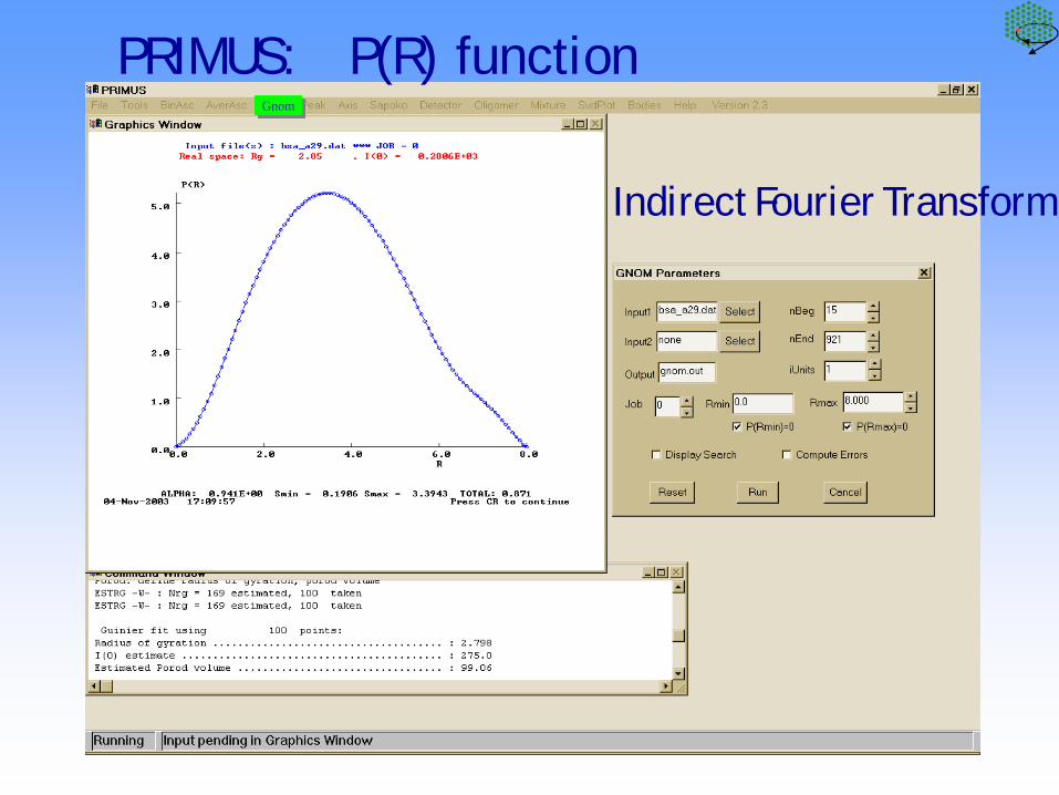
Real/reciprocal space transformation
p(r)=r2 γ(r) distance distribution functionγ0(r)=γ(r)/γ(0)
Probability to find a point at distance r from a given point
inside the particle
i
j
rij

Distance distribution function from simple shapes

Distance distribution function of helix
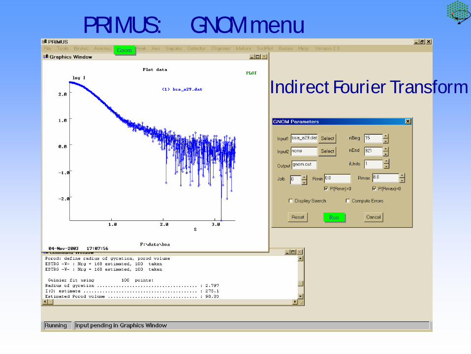
Gnom
Run
PRIMUS: GNOM menu
Indirect Fourier Transform
Gnom
PRIMUS: P(R) function
Indirect Fourier Transform
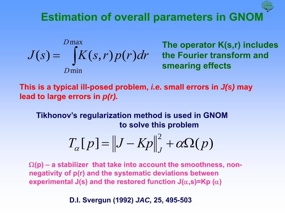
∫=max
min
)(),()(D
D
drrprsKsJThe operator K(s,r) includes the Fourier transform and smearing effects
This is a typical ill-posed problem, i.e. small errors in J(s) may lead to large errors in p(r).
Tikhonov’s regularization method is used in GNOM to solve this problem
)(][ 2 pKpJpTJ
Ω+−= αα
Ω(p) – a stabilizer that take into account the smoothness, non-negativity of p(r) and the systematic deviations between experimental J(s) and the restored function J(α,s)=Kp (α)
D.I. Svergun (1992) JAC, 25, 495-503
Estimation of overall parameters in GNOM
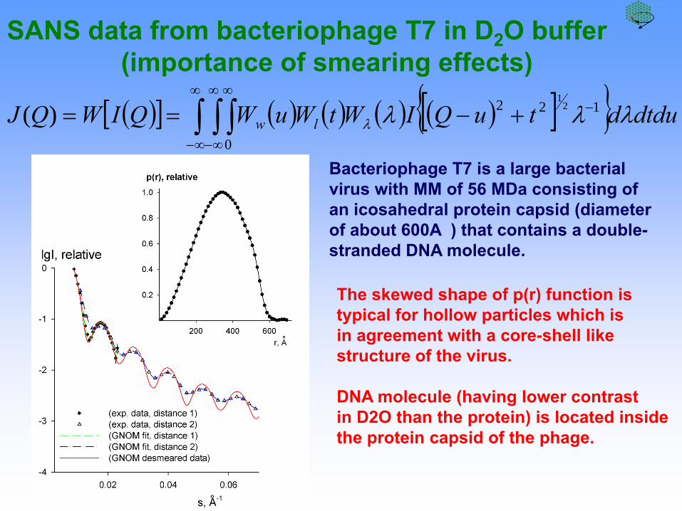
SANS data from bacteriophage T7 in D2O buffer(importance of smearing effects)
Bacteriophage T7 is a large bacterial virus with MM of 56 MDa consisting of an icosahedral protein capsid (diameter of about 600A ) that contains a double-stranded DNA molecule.
The skewed shape of p(r) function is typical for hollow particles which is in agreement with a core-shell like structure of the virus.
DNA molecule (having lower contrast in D2O than the protein) is located inside the protein capsid of the phage.
( )[ ] ( ) ( ) ( ) ( )[ ]{ }∫ ∫ ∫∞
∞−
∞
∞−
∞−+−==
0
122 21
)( dtdudtuQIWtWuWQIWQJ lw λλλλ
♦ In the original version of GNOM the maximum particle size Dmax is a user-defined parameter and successive calculations with different Dmax are required to select its optimum value.
AUTOGNOM – automated version of GNOM for monodisperse systems
♦ This optimum Dmax should provide a smooth real space distance distribution function p(r) such that p(Dmax) and its first derivative p'(Dmax) are approaching zero, and the back-transformed intensity from the p(r)fits the experimental data.
Petoukhov, M.V., Konarev, P.V., Kikhney, A.G. & Svergun, D.I.
(2007) J. Appl. Cryst., 40, s223-s228.

Estimation of Dmax with GNOM (under-estimation)
6.0
Poor fit to experimental data
Distance distribution function p(r)goes to zero too abruptly
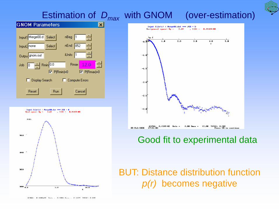
Estimation of Dmax with GNOM (over-estimation)
Good fit to experimental data
BUT: Distance distribution function p(r) becomes negative
12.0

8.0
Estimation of Dmax with GNOM (correct case)
Good fit to experimental data
Distance distribution function p(r)goes smoothly to zero

♦ The maximum size is determined from automated comparison of the p(r) functions calculated at different Dmax values ranging from 2Rg to 4Rg, where Rg is the radius of gyration provided by AUTORG.
AUTOGNOM – automated version of GNOM for monodisperse systems
♦The calculated p(r) functions and corresponding fits to the experimental curves are compared using the perceptual criteria of GNOM (Svergun, 1992) together with the analysis of the behavior of p(r) function near Dmax and the best p(r) function is chosen for the final output.
Petoukhov, M.V., Konarev, P.V., Kikhney, A.G. & Svergun, D.I.
(2007) J. Appl. Cryst., 40, s223-s228.

An automated SAXS pipeline at P12
Data normalization2D-1D reductionData processingCheck for radiation damageComputation of overall parameters Database search Ab initio modellingXML-summary file generation
Hardware-independent analysis block
Kratky plot
This provides a sensitive means of monitoring the degree of compactness of a protein as a function of a given parameter.
This is most conveniently represented using the so-called
Kratky plot of s2I(s) vs s.Globular particle : bell-shaped curve
Gaussian chain : plateau at large s-values
but beware: a plateau does not imply a Gaussian chain

SAXS patterns of globular and flexible proteins
Natively unfolded
Globular
Multidomain with flexible linkers

Summary of model-independent information
I(0)/c, i.e. molecular mass (from Guinier plot or p(r) function)
Radius of gyration Rg (from Guinier plot or p(r) function)
Radii of gyration of thickness or cross-section (anisometrc particles)
Maximum particle size Dmax (from p(r) function)
Particle volume V (from I(0) and Porod invariant)
Globular or unfoded (From Kratky plot)

Thank you!
Top Related