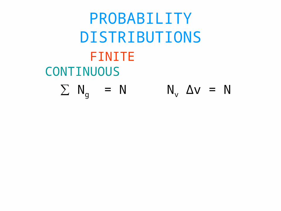
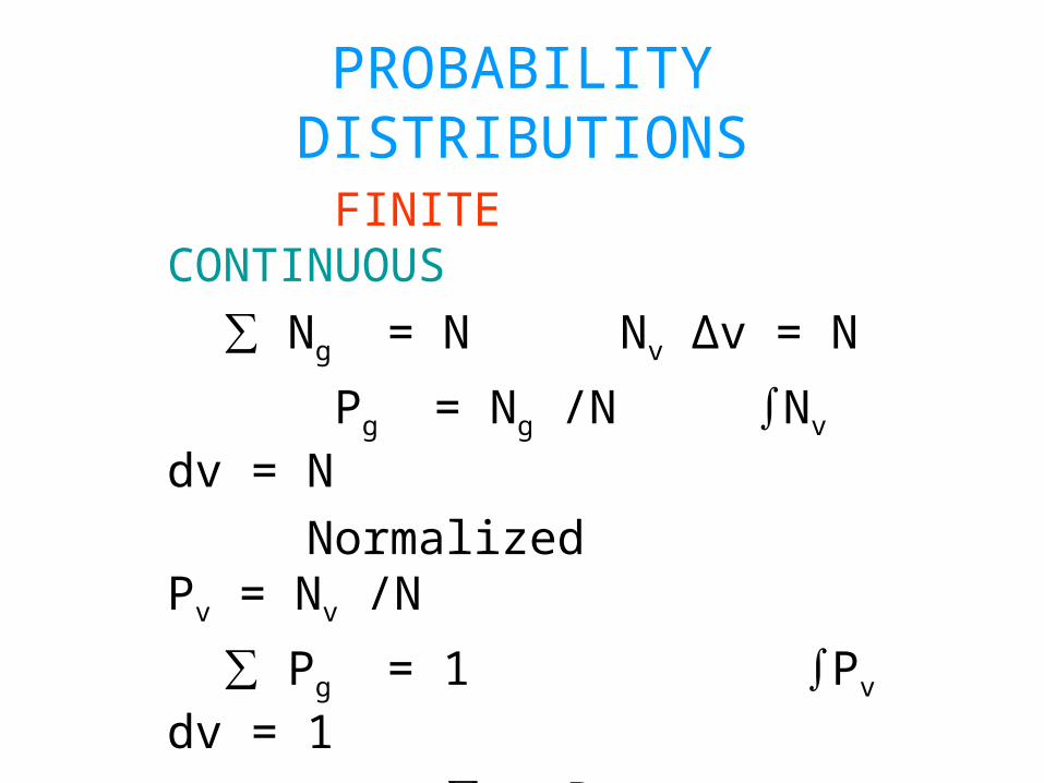
PROBABILITY DISTRIBUTIONS

FINITE CONTINUOUS

∑ Ng = N Nv Δv = N

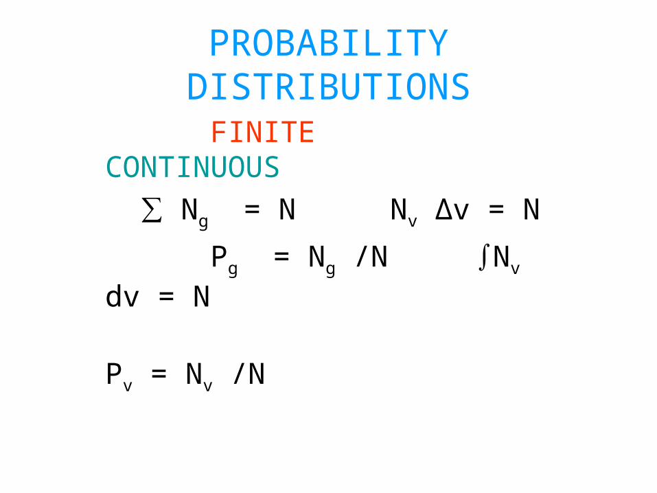
PROBABILITY DISTRIBUTIONS

FINITE CONTINUOUS

∑ Ng = N Nv Δv = N

Pg = Ng /N ∫Nv dv = N

Pv = Nv /N

PROBABILITY DISTRIBUTIONS

FINITE CONTINUOUS

∑ Ng = N Nv Δv = N

Pg = Ng /N ∫Nv dv = N

Normalized Pv = Nv /N

∑ Pg = 1 ∫Pv dv = 1

PROBABILITY DISTRIBUTIONS

FINITE CONTINUOUS

∑ Ng = N Nv Δv = N

Pg = Ng /N ∫Nv dv = N

Normalized Pv = Nv /N

∑ Pg = 1 ∫Pv dv = 1

< g> = ∑ g Pg < v > = ∫vPv dv

PROBABILITY DISTRIBUTIONS

FINITE CONTINUOUS

∑ Ng = N Nv Δv = N

Pg = Ng /N ∫Nv dv = N

Normalized Pv = Nv /N

∑ Pg = 1 ∫Pv dv = 1

< g> = ∑ g Pg < v > = ∫vPv dv

<g2> = ∑ g2 Pg < v2> = ∫v2 Pv dv

Velocity Distribution of Gases

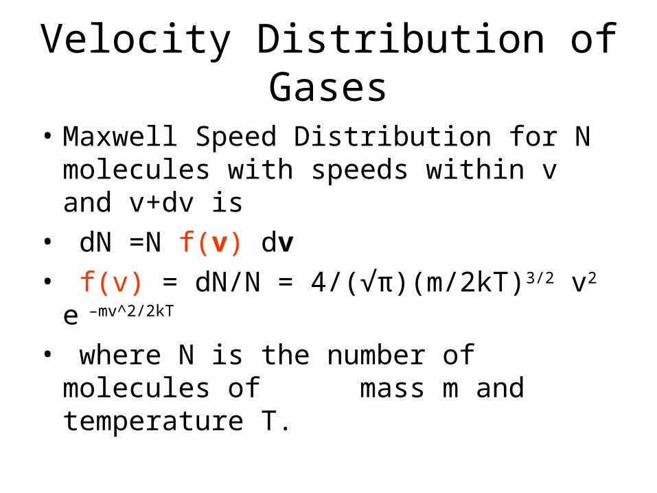
• Maxwell Speed Distribution for N molecules with speeds within v and v+dv is

Velocity Distribution of Gases

• Maxwell Speed Distribution for N molecules with speeds within v and v+dv is

• dN =N f(v) dv

Velocity Distribution of Gases

• Maxwell Speed Distribution for N molecules with speeds within v and v+dv is

• dN =N f(v) dv

• f(v) = dN/N = 4/(√π)(m/2kT)3/2 v2 e –mv^2/2kT

Velocity Distribution of Gases

• Maxwell Speed Distribution for N molecules with speeds within v and v+dv is

• dN =N f(v) dv

• f(v) = dN/N = 4/(√π)(m/2kT)3/2 v2 e –mv^2/2kT

• where N is the number of molecules of mass m and temperature T.

Velocity Distribution of Gases

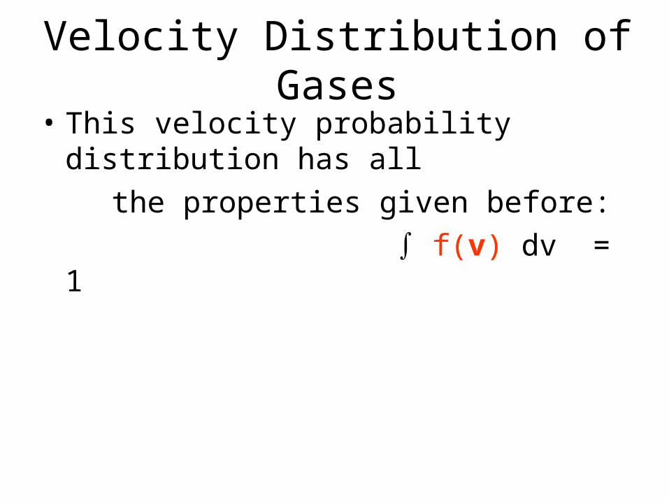
• This velocity probability distribution has all

the properties given before:

∫ f(v) dv = 1

Velocity Distribution of Gases

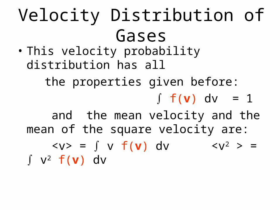
• This velocity probability distribution has all

the properties given before:

∫ f(v) dv = 1

and the mean velocity and the mean of the square velocity are:

<v> = ∫ v f(v) dv <v2 > = ∫ v2 f(v) dv

Velocity Distribution of Gases

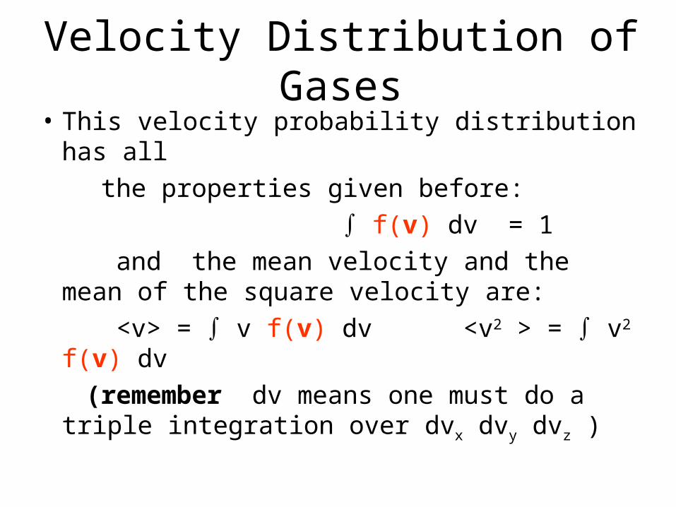
• This velocity probability distribution has all

the properties given before:

∫ f(v) dv = 1

and the mean velocity and the mean of the square velocity are:

<v> = ∫ v f(v) dv <v2 > = ∫ v2 f(v) dv

(remember dv means one must do a triple integration over dvx dvy dvz )

Velocity Distribution of Gases

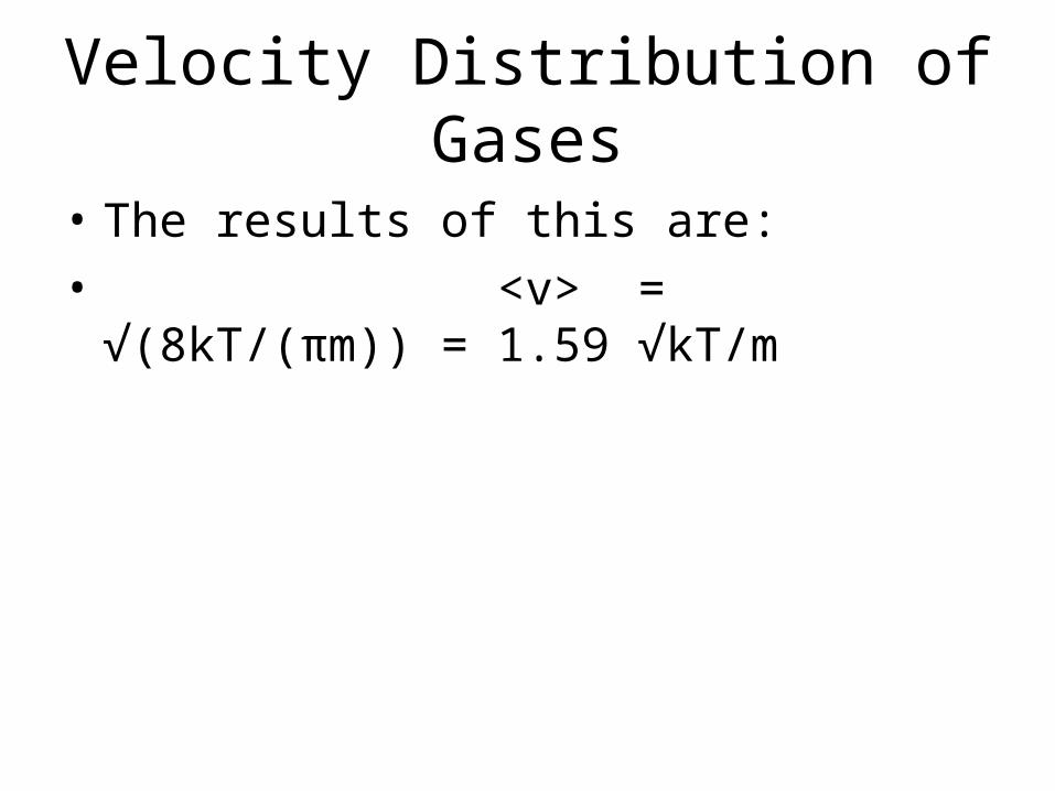
• The results of this are:

• <v> = √(8kT/(πm)) = 1.59 √kT/m

Velocity Distribution of Gases

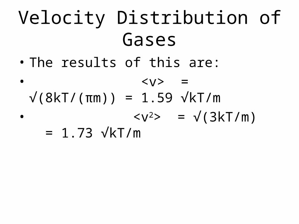
• The results of this are:

• <v> = √(8kT/(πm)) = 1.59 √kT/m

• <v2> = √(3kT/m) = 1.73 √kT/m

Velocity Distribution of Gases

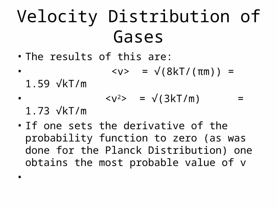
• The results of this are:

• <v> = √(8kT/(πm)) = 1.59 √kT/m

• <v2> = √(3kT/m) = 1.73 √kT/m

• If one sets the derivative of the probability function to zero (as was done for the Planck Distribution) one obtains the most probable value of v

•

Velocity Distribution of Gases

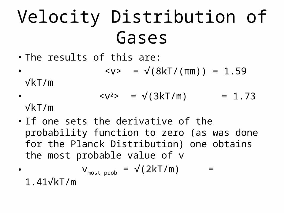
• The results of this are:

• <v> = √(8kT/(πm)) = 1.59 √kT/m

• <v2> = √(3kT/m) = 1.73 √kT/m

• If one sets the derivative of the probability function to zero (as was done for the Planck Distribution) one obtains the most probable value of v

• vmost prob = √(2kT/m) = 1.41√kT/m

Maxwell-Boltzmann Distribution

• Molecules with more complex shape have internal molecular energy.

Maxwell-Boltzmann Distribution

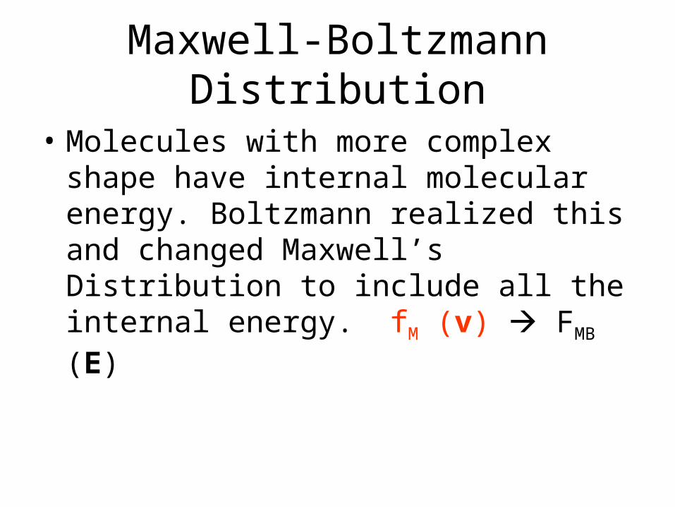
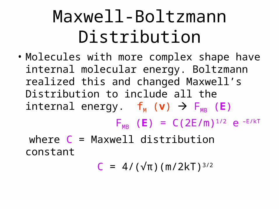
• Molecules with more complex shape have internal molecular energy. Boltzmann realized this and changed Maxwell’s Distribution to include all the internal energy. fM (v) FMB (E)

Maxwell-Boltzmann Distribution

• Molecules with more complex shape have internal molecular energy. Boltzmann realized this and changed Maxwell’s Distribution to include all the internal energy. fM (v) FMB (E)

FMB (E) = C(2E/m)1/2 e –E/kT

where C = Maxwell distribution constant

C = 4/(√π)(m/2kT)3/2

Maxwell-Boltzmann Distribution

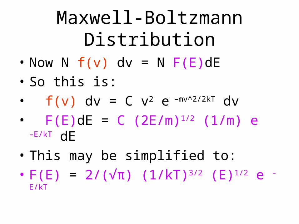
• Now N f(v) dv = N F(E)dE

• So this is:

• f(v) dv = C v2 e –mv^2/2kT dv

• F(E)dE = C (2E/m)1/2 (1/m) e –E/kT dE

• This may be simplified to:

• F(E) = 2/(√π) (1/kT)3/2 (E)1/2 e -E/kT

Maxwell-Boltzmann Distribution

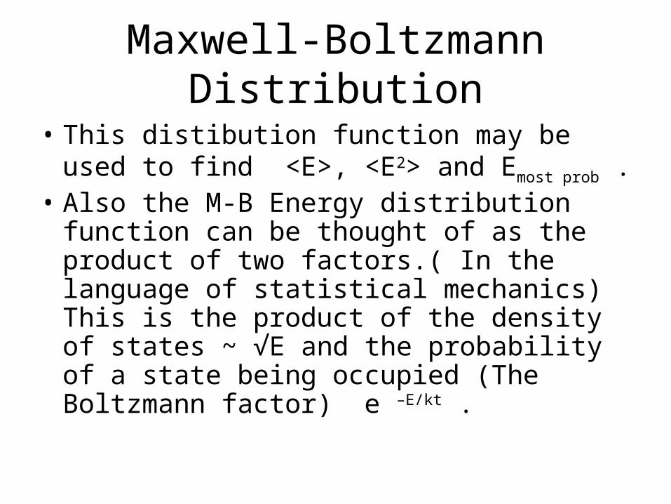
• This distibution function may be used to find <E>, <E2> and Emost prob .

• Also the M-B Energy distribution function can be thought of as the product of two factors.( In the language of statistical mechanics) This is the product of the density of states ~ √E and the probability of a state being occupied (The Boltzmann factor) e –E/kt .

MOLECULAR INTERNAL ENERGY

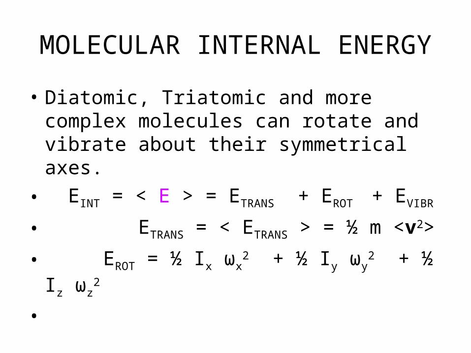
• Diatomic, Triatomic and more complex molecules can rotate and vibrate about their symmetrical axes.

•

MOLECULAR INTERNAL ENERGY

• Diatomic, Triatomic and more complex molecules can rotate and vibrate about their symmetrical axes.

• EINT = < E > = ETRANS + EROT + EVIBR

•

MOLECULAR INTERNAL ENERGY

• Diatomic, Triatomic and more complex molecules can rotate and vibrate about their symmetrical axes.

• EINT = < E > = ETRANS + EROT + EVIBR

• ETRANS = < ETRANS > = ½ m <v2>

•

MOLECULAR INTERNAL ENERGY

• Diatomic, Triatomic and more complex molecules can rotate and vibrate about their symmetrical axes.

• EINT = < E > = ETRANS + EROT + EVIBR

• ETRANS = < ETRANS > = ½ m <v2>

• EROT = ½ Ix ωx2 + ½ Iy ωy

2 + ½ Iz ωz2

•

MOLECULAR INTERNAL ENERGY

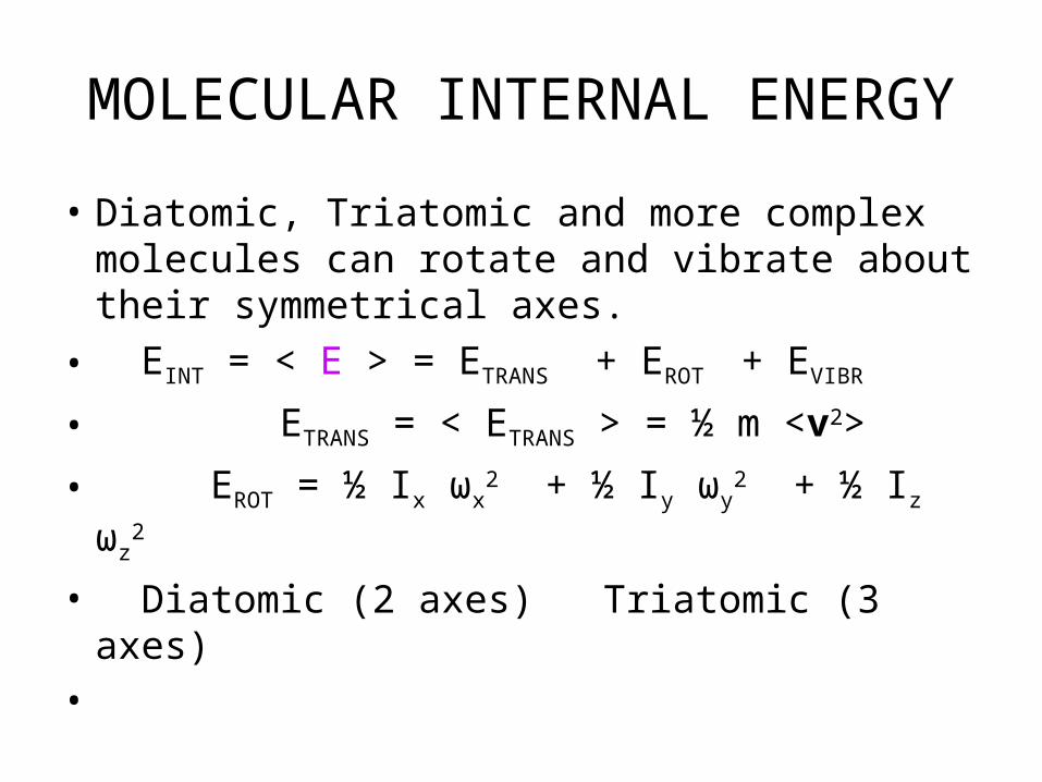
• Diatomic, Triatomic and more complex molecules can rotate and vibrate about their symmetrical axes.

• EINT = < E > = ETRANS + EROT + EVIBR

• ETRANS = < ETRANS > = ½ m <v2>

• EROT = ½ Ix ωx2 + ½ Iy ωy

2 + ½ Iz ωz2

• Diatomic (2 axes) Triatomic (3 axes)

•

MOLECULAR INTERNAL ENERGY

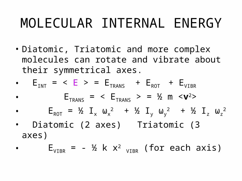
• Diatomic, Triatomic and more complex molecules can rotate and vibrate about their symmetrical axes.

• EINT = < E > = ETRANS + EROT + EVIBR

• ETRANS = < ETRANS > = ½ m <v2>

• EROT = ½ Ix ωx2 + ½ Iy ωy

2 + ½ Iz ωz2

• Diatomic (2 axes) Triatomic (3 axes)

• EVIBR = - ½ k x2 VIBR (for each axis)

INTERNAL MOLECULAR ENERGY

• For a diatomic molecule then <E> = 5/2 kT

INTERNAL MOLECULAR ENERGY

• For a diatomic molecule then <E> = 5/2 kT

• One of the basic principles used in the Kinetic Theory of Gases is that each degree of freedom has an average energy

• of ½ kT.

INTERNAL MOLECULAR ENERGY

• For a diatomic molecule then <E> = 5/2 kT

• One of the basic principles used in the Kinetic Theory of Gases is that each degree of freedom has an average energy

• of ½ kT. Or <E> = (s/2) kT

INTERNAL MOLECULAR ENERGY

• For a diatomic molecule then <E> = 5/2 kT

• One of the basic principles used in the Kinetic Theory of Gases is that each degree of freedom has an average energy

• of ½ kT. Or <E> = (s/2) kT

where s = the number of degrees of freedom

INTERNAL MOLECULAR ENERGY

• For a diatomic molecule then <E> = 5/2 kT

• One of the basic principles used in the Kinetic Theory of Gases is that each degree of freedom has an average energy

• of ½ kT. Or <E> = (s/2) kT

where s = the number of degrees of freedom

• This is called the

• EQUIPARTION THEOREM

INTERNAL MOLECULAR ENERGY

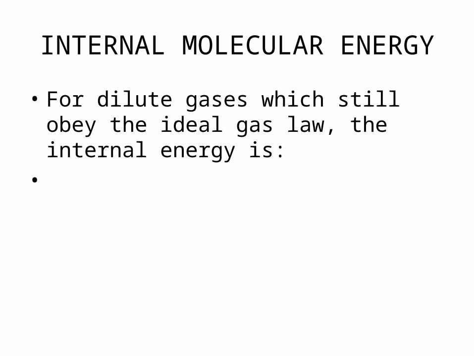
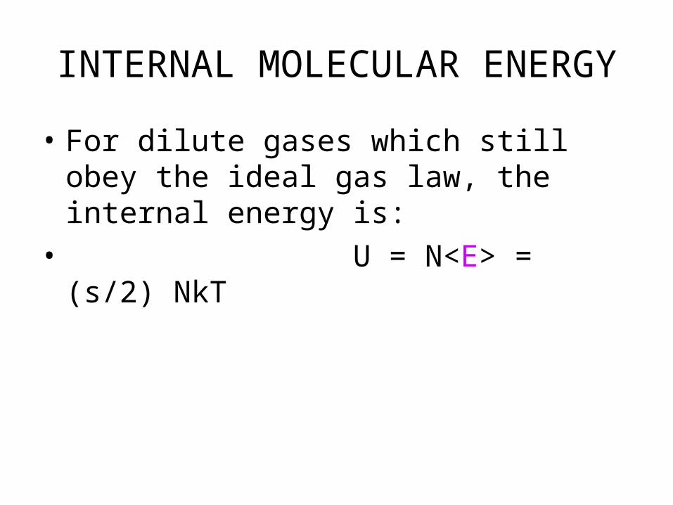
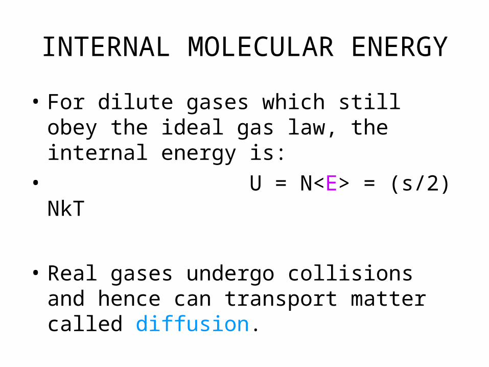
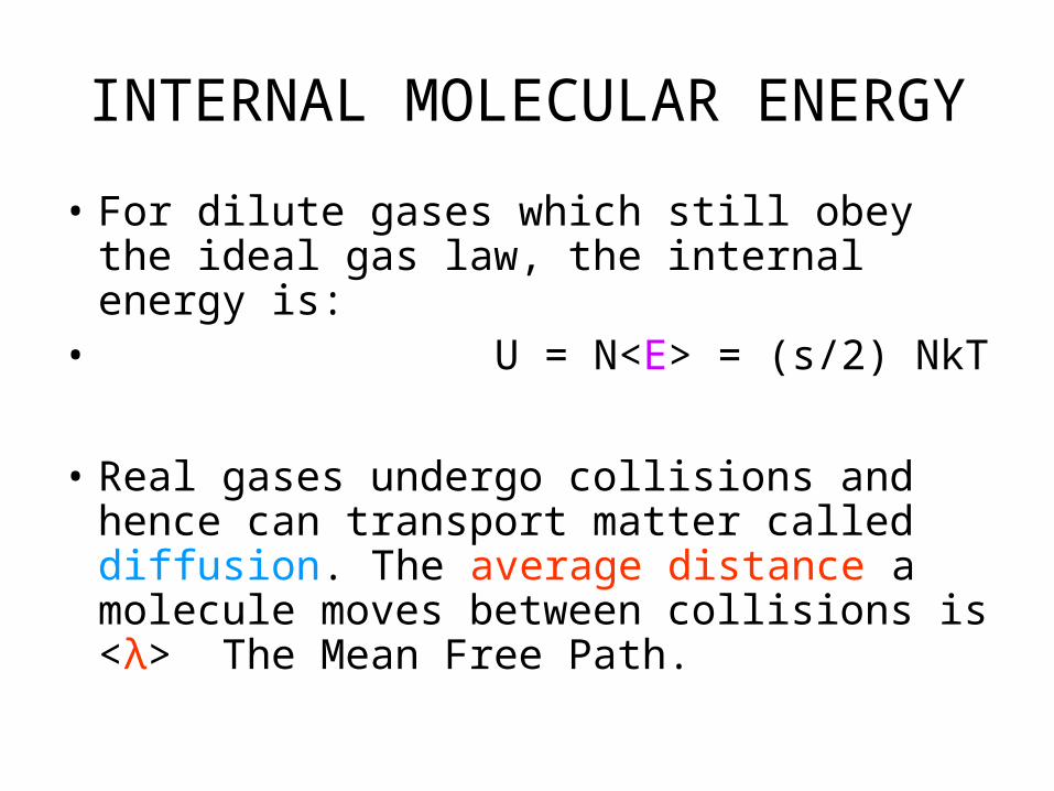
• For dilute gases which still obey the ideal gas law, the internal energy is:

•

INTERNAL MOLECULAR ENERGY

• For dilute gases which still obey the ideal gas law, the internal energy is:

• U = N<E> = (s/2) NkT

INTERNAL MOLECULAR ENERGY

• For dilute gases which still obey the ideal gas law, the internal energy is:

• U = N<E> = (s/2) NkT

• Real gases undergo collisions and hence can transport matter called diffusion.

INTERNAL MOLECULAR ENERGY

• For dilute gases which still obey the ideal gas law, the internal energy is:

• U = N<E> = (s/2) NkT

• Real gases undergo collisions and hence can transport matter called diffusion. The average distance a molecule moves between collisions is <λ> The Mean Free Path.

COLLISIONS OF MOLECULES

• Let D be the diameter of a molecule.

COLLISIONS OF MOLECULES

• Let D be the diameter of a molecule. The collision cross section is merely the cross-sectional area σ = π D2 .

COLLISIONS OF MOLECULES

• Let D be the diameter of a molecule. The collision cross section is merely the cross-sectional area σ = π D2 . If there is a collision then the molecule traveles a distance λ = vt.

COLLISIONS OF MOLECULES

• Let D be the diameter of a molecule. The collision cross section is merely the cross-sectional area σ = π D2 . If there is a collision then the molecule traveles a distance λ = vt. If one averages this

• <λ> = vRMS τ

where τ = mean collision time.

COLLISIONS OF MOLECULES

• Let D be the diameter of a molecule. The collision cross section is merely the cross-sectional area σ = π D2 . If there is a collision then the molecule travels a distance λ = vt. If one averages this

• <λ> = vRMS τ

where τ = mean collision time. During this time there are N collisions in a volume V.

MOLECULAR COLLISIONS

• The molecule sweeps out a volume which is V = AvRMSτ =

MOLECULAR COLLISIONS

• The molecule sweeps out a volume which is V = AvRMSτ = σ vRMSτ

MOLECULAR COLLISIONS

• The molecule sweeps out a volume which is V = AvRMSτ = σ vRMSτ Since there are number / volume (ndens ) molecules undergoing a collision then the average number of collisions per unit time is

τ = 1/N

MOLECULAR COLLISIONS

• The molecule sweeps out a volume which is V = AvRMSτ = σ vRMSτ Since there are number / volume (ndens ) molecules undergoing a collision then the average number of collisions per unit time is

τ = 1/N = 1/(nV/τ)

MOLECULAR COLLISIONS

• The molecule sweeps out a volume which is V = AvRMSτ = σ vRMSτ Since there are number / volume (ndens ) molecules undergoing a collision then the average number of collisions per unit time is

τ = 1/N = 1/(nV/τ) = 1/nσ vRMS .

MOLECULAR COLLISIONS

• The molecule sweeps out a volume which is V = AvRMSτ = σ vRMSτ Since there are number / volume (ndens ) molecules undergoing a collision then the average number of collisions per unit time is

τ = 1/N = 1/(nV/τ) = 1/nσ vRMS .

However, both molecules are moving and this increases the velocity by √ 2.

MOLECULAR COLLISIONS

• Thus τ = 1/ (√2 nσvRMS )

MOLECULAR COLLISIONS

• Thus τ = 1/ (√2 nσvRMS )

• and

<λ> = vRMS τ = 1/(√2 nσ)

MOLECULAR COLLISIONS

• Thus τ = 1/ (√2 nσvRMS )

• and

<λ> = vRMS τ = 1/(√2 nσ)

In 1827 Robert Brown observed small particles moving in a suspended atmosphere. This was later hypothesised to be due to collisions by gas molecules.

MOLECULAR COLLISIONS

• The movement of these particles was observed to be random and was similar to the mathematical RANDOM WALK problem.

MOLECULAR COLLISIONS

• The movement of these particles was observed to be random and was similar to the mathematical RANDOM WALK problem. See the link below:

• http://www.aip.org/history/einstein/brownian.htm

MOLECULAR COLLISIONS

• The movement of these particles was observed to be random and was similar to the mathematical RANDOM WALK problem. See the link below:

• http://www.aip.org/history/einstein/brownian.htm

• Also click on the Essay on Einstein Brownian Motion.

MOLECULAR COLLISIONS

• Each of the distances moved by the molecules is L, because of the possibility of positive and negative directions it is best to calculate the < R2 > = N L2

MOLECULAR COLLISIONS

• Each of the distances moved by the molecules is L, because of the possibility of positive and negative directions it is best to calculate the < R2 > = N L2

where N is the number of steps or collisions.

MOLECULAR COLLISIONS

• Each of the distances moved by the molecules is L, because of the possibility of positive and negative directions it is best to calculate the < R2 > = N L2

where N is the number of steps or collisions.

• Since there are N collisions in a time t

• t = Nτ

MOLECULAR COLLISIONS

• Each of the distances moved by the molecules is L, because of the possibility of positive and negative directions it is best to calculate the < R2 > = N L2

where N is the number of steps or collisions.

• Since there are N collisions in a time t

• t = Nτ so in the above equation

< R2 > = (t/τ) λ2