ISSN 1 746-7233, England, UKWorld Journal of Modelling and Simulation

Vol. 9 (2013) No. 2, pp. 139-149

Numerical Behavior of a Fractional Order HIV/AIDS Epidemic Model

Mohammad Javidi1∗ , Nemat Nyamoradi2

Department of Mathematics, Faculty of Sciences, Razi University, Kermanshah 67149, Iran

(Received April 18 2012, Revised September 30 2012, Accepted April 16 2013)

Abstract. In this paper, a fractional order HIV/AIDS (FOHA) epidemic model with treatment is investigated.The first step in the proposed procedure is represent the FOHA system as an equivalent system of ordinarydifferential equations. In the second step, we solved the system obtained in the first step by using the wellknown fourth order Runge-Kutta method. Numerical simulations are also presented to verify the obtainedresults. We solved the FOHA system for 0.8 ≤ α < 1.

Keywords: HIV/AIDS epidemic model, fractional order, numerical method

1 Introduction

South Africa is currently experiencing a serious HIV/AIDS epidemic in history. Nearly, one in every fiveSouth Africans is infected with HIV, corresponding to approximately 5.7 million individuals. Mathematicalmodels have been used to model the dynamics of HIV/AIDS. Many researchers discussed on this models.Nyabadza [13], proposed a simple deterministic HIV/AIDS model incorporating sexual partner acquisition,behavior change and treatment as HIV/AIDS control strategies is formulated using a system of ordinary differ-ential equations with the object of applying it to the current South African situation. Samanta [34], considereda nonautonomous stage-structured HIV/AIDS epidemic model having two stages of the period of infectionaccording to the developing progress of infection before AIDS defined in, with varying total population sizeand distributed time delay to become infectious. The authors of [39], proposed a SIR mathematical modelof HIV transmission dynamics to explain the epidemiology of infectious diseases, and to assess the poten-tial benefits of proposed control strategies. A general SIR model is considered where there is no interventionand that resulted to an endemic situation. Also the same authors [38], examined and extended the HIV/AIDSmodel incorporating complacency by Flugentius et al for the adult population. Complacency is assumed afunction of the number of AIDS cases in a population with an inverse relation. Zunyou and coauthors [36],reviews the epidemic of HIV infection and AIDS, the Chinese national policy development in response to theepidemic, and disparities between policies and the need for AIDS prevention in China. Dynamic models andcomputer simulations are experimental tools for comparing regions or risk groups, testing theories, assessingquantitative conjectures, and answering questions [16]. Also see [2, 5, 7, 28, 33].

The authors of [1], reviews various mathematical models already proposed in the context of HIV trans-mission and the AIDS epidemic. Emphasis is placed on the various forms of HIV transmission models andthe assumptions under which the models were based. We also trace how transmission models evolved fromthe simplest population of homosexuals with homogeneity with respect to susceptibility, infectiousness andsexual mixing. Some HIV transmission dynamics models are stochastic, with probabilities of moving to thenext stage at each time step. Stochastic models assume that the response variables are a family of randomvariables indexed by time so that the HIV epidemic is a stochastic process [37].

∗ Corresponding author. E-mail address: mo javidi@yahoo.com.

Published by World Academic Press, World Academic Union

140 M. Javidi & N. Nyamorady: Numerical Behavior of a Fractional Order HIV/AIDS

AIDS has developed into a global pandemic since the first patients were identified in 1981. Since 1999,the year in which it is thought that the epidemic peaked, globally, the number of new infections has fallenby 19%. Of the estimated 15 million people living with HIV in middle-income countries who need treatmenttoday, 5.2 million have accesstranslating into fewer AIDS-related deaths. For the estimated 33.3 million peopleliving with HIV after nearly 30 years into a very complex epidemic, the gains are real but still fragile.

In 2009 alone, 1.2 million people received HIV antiretroviral therapy for the first time an increase inthe number of people receiving treatment of 30% in a single year. Overall, the number of people receivingtherapy has grown 13-fold, more than five million people in middle-income countries, since 2004. Expandingaccess to treatment has contributed to a 19% decline in deaths among people living with HIV between 2004and 2009. This is just the beginning: 10 million people living with HIV who are eligible for treatment underthe new WHO guidelines are still in need. Also, it is reported that 33.3 million people currently live withHIV-1 infection, 2.6 million people have been newly infected and 1.8 million AIDS deaths occurred in 2009(http://www.unaids.org/epi/2005/index.asp). It is well known that HIV mainly targets a host’s CD4+ T -cells,the main driver of the immune response. Chronic HIV infection causes gradual depletion of the CD4+ T -cellpool, and thus progressively compromises the host’s immune response, leading to humoral and cellular im-mune function loss (the marker of the on set of AIDS), making the host susceptible to opportunistic infections.The fact that HIV replicates rapidly, producing on average 1010 viral particles per day, led to the realizationthat HIV evolves so rapidly that treatment with a single drug is bound to fail [30]. In a normal healthy in-dividual’s peripheral blood, the level of CD4+ T -cells is between 800mm−3 and 1200mm−3 and once thisnumber reaches 200 or below in an HIV infected patient, the person is classified as having AIDS. Without drugtreatment, HIV-1 infection is nearly uniformly fatal within 5-10 years. With drug therapies, such as HAART(highly active antiretroviral therapy), treated individuals can live longer free of HIV-related symptoms [35].

Fractional differential equations have gained considerable importance due to their application in varioussciences, such as physics, mechanics, chemistry, engineering [6, 8, 17, 20–24, 26]. In the recent years, the dynamicbehaviors of fractional-order differential systems have received increasing attention.

The existence of solutions of initial value problems for fractional order differential equations have beenstudied in the literature [14, 19, 31, 32] and the references therein.

In this paper, we first introduce a fractional order HIV/AIDS epidemic model with treatment. We ex-plained a numerical method to converting the system of fractional differential equations to system of ordinarydifferential equations. Finally, numerical simulations are presented to illustrate the obtained results.

2 Preliminaries

Definition 1. The Riemann-Liouville fractional integral operator of order α > 0, of function f ∈ L1(R+) isdefined as

Iαt0f(t) =

1Γ (α)

∫ t

t0

(t− s)α−1f(s)ds,

where Γ (·) is the Euler gamma function.

Definition 2. The Riemann-Liouville fractional derivative of order α > 0, n − 1 < α < n, n ∈ N is definedas

Dαt0f(t) =

1Γ (n− α)

( ddt

)n∫ t

t0

(t− s)n−α−1f(s)ds,

where the function f(t) have absolutely continuous derivatives up to order (n− 1).

The initial value problem related to Definition 2 isDαx(t) = f(t, x(t)),x(t)|t=0+ = x0,

(1)

WJMS email for contribution: submit@wjms.org.uk

World Journal of Modelling and Simulation, Vol. 9 (2013) No. 2, pp. 139-149 141

where 0 < α < 1 and Dα = Dα0 .

In [9] the following results about the existence and uniqueness of solutions for Eq. (1) are further pre-sented.

Theorem 1. Assume that < : [0, T ∗]× [x0−δ, x0 +δ] with some T ∗ > 0 and some δ > 0, and let the function

f : < → R be continuous. Furthermore, define T := minT ∗,

( δΓ (α+1)||f ||∞

) 1α

, then there exists a function

x : [0, T ] → R solving the initial value problem (1). Notice that ||f ||∞ is the norm of function f .

Theorem 2. Assume that < : [0, T ∗]× [x0−δ, x0 +δ] with some T ∗ > 0 and some δ > 0, and let the functionf : < → R be bounded on < and fulfill a Lipschitz condition with respect to the second variable, i.e.

|f(t, x)− f(t, y)| ≤ L|x− y|

with some constant number L > 0 independent of t, x, y. Then denoting T as Theorem 1, there exists at mostone function x : [0, T ] → R solving the initial value problem Eq. (1).

Furthermore, the above definition in one dimension can naturally be generalized to the case of multipledimensions. That is, let X(t) = (x1(t), x2(t), · · · , xn(t))T ∈ Rn and α = (α1, α2, · · · , αn)T ∈ Rn, 0 <αi < 1, i = 1, 2, · · · , n. The n-dimension FODE is described as follows:

DαX(t) =1

Γ (1− α)

∫ t

0

X ′(u)(t− u)α

du , F (t,X(t)), (2)

where

1Γ (1− α)

∫ t

0

X ′(u)(t− u)α

du = (Dα1x1(t), Dα2x2(t), · · · , Dαnxn(t))T

and

F (t,X(t)) =

f1(t, x1(t), x2(t), · · · , xn(t))f2(t, x1(t), x2(t), · · · , xn(t))

...fn(t, x1(t), x2(t), · · · , xn(t))

.

The results of Theorems 1, 2 can be easily generalizes to the initial value problem of the vector-value Eq.(2).

3 Fractional order hiv/aids model

To construct the model, we first divide the total population into a susceptible class of size S and aninfectious class before the onset of AIDS and a full-blown AIDS group of size A which is removed from theactive population. Based on the facts that the infectious period is very long (≥ 10 years), we further considerseveral stages of the infectious period. For simplicity, we only consider two stages according to clinic stagesand papers [15, 35]i.e., the asymptomatic phase (I) and the symptomatic phase (J). Thus, we first establish thefollowing model:

dαSdtα = µK − cβ(I + bJ)S − µS,dαIdtα = cβ(I + bJ)S − (µ+ k1)I + γJ,dαJdtα = k1I − (µ+ k2 + γ)J,dαAdtα = k2J − (µ+ d)A,

(3)

S(δ) = S0, I(δ) = I0, J(δ) = J0, A(δ) = A0, (4)

WJMS email for subscription: info@wjms.org.uk

142 M. Javidi & N. Nyamorady: Numerical Behavior of a Fractional Order HIV/AIDS

where, µK is the recruitment rate of the population, µ is the number of death rate constant. c is the averagenumber of contacts of an individual per unit of time. β and bβ are probability of disease transmission percontact by an infective in the first stage and in the second stage, respectively. k1 and k2 are transfer rateconstant from the asymptomatic phase I to the symptomatic phase J and from the symptomatic phase to theAIDS cases, respectively. γ is treatment rate from the symptomatic phase J to the asymptomatic phase I . d isthe disease-related death rate of the AIDS cases.

Now, some stability theorems on fractional-order systems and their related results are introduced. Thefirst theorem has been given for commensurate fractional-order linear systems.

Theorem 3. ([27]) The following autonomous system:

dαx

dtα= Ax, x(0) = x0, (5)

with 0 < α ≤ 1, x ∈ Rn and A ∈ Rn×n, is asymptotically stable if and only if | arg(λ)| > απ2 is satisfied

for all eigenvalues of matrix A. Also, this system is stable if and only if | arg(λ)| ≥ απ2 is satisfied for all

eigenvalues of matrixAwith those critical eigenvalues satisfying | arg(λ)| = απ2 having geometric multiplicity

of one. The geometric multiplicity of an eigenvalue λ of the matrixA is the dimension of the subspace of vectorsv for which Av = λv.

Theorem 4. ([9]). Consider the following commensurate fractional-order system:

dαx

dtα= f(x), x(0) = x0, (6)

with 0 < α ≤ 1 and x ∈ Rn. The equilibrium points of system Eq. (6) are calculated by solving the followingequation: f(x) = 0. These points are locally asymptotically stable if all eigenvalues λi of the Jacobian matrixJ = ∂f

∂x evaluated at the equilibrium points satisfy: | arg(λi)| > απ2 .

According to [[11], Theorem 2], the basic reproduction number of system Eq.(3) is

R0 =cβK(µ+ k2 + γ + bk1)(µ+ k1)(µ+ k2) + µγ

. (7)

3.1 Equilibrium points and stability

To evaluate the equilibrium points of Eq. (3), let

dαS

dtα= 0,

dαI

dtα= 0,

dαJ

dtα= 0,

dαA

dtα= 0.

Then the equilibrium points are E0 = (K, 0, 0, 0) and E1 = (S, I, J , A) for R0 > 1, where

S =(µ+ k1)(µ+ k2) + µγ

cβ(µ+ k2 + γ + bk1), I =

(µ+ k2 + γ)µK(µ+ k1)(µ+ k2) + µγ

(1− 1

R0

),

J =k1

(µ+ k2 + γ)I , A =

k2

µ+ dJ.

The Jacobian matrix J(E0) for the system given in Eq. (3) evaluated at the disease free equilibrium is asfollows:

J(E0) =

−µ −cβK −cβbK 00 cβK − (µ+ k1) cβbK + γ 00 k1 −(µ+ k2 + γ) 00 0 k2 −(µ+ d)

.

WJMS email for contribution: submit@wjms.org.uk

World Journal of Modelling and Simulation, Vol. 9 (2013) No. 2, pp. 139-149 143

Theorem 5. ([29]) The disease free equilibrium E0 of system Eq. (3) is asymptotically stable if R0 < 1. IfR0 > 1, then E0 is unstable.

We now discuss the asymptotic stability of the equilibrium E1 of the system Eq. (3).The characteristic equation of the linearized system is in the form

P (λ) = −(λ+ µ+ d)R(λ) = 0, (8)

with R(λ) = λ3 +A1λ2 +A2λ+A3, The coefficients A1, A2 and A3 calculated in [29].

Let D(R) denote the discriminant of a polynomial R(λ). Then

D(R) = 18A1A2A3 + (A1A2)2 − 4A3A31 − 4A3

2 − 27A33.

Using the proposition given in [12], we have the following result.

Theorem 6. ([29]) The equilibrium point E1 of the system Eq. (3) is asymptotically stable if one of the fol-lowing conditions holds for polynomial R which is given as in Eq. (8):(i) D(R) > 0, A1 > 0, A3 > 0 and A1A2 > A3 (Routh-Hurwitz conditions ).(ii) D(R) < 0, A1 ≥ 0, A2 ≥ 0, A3 > 0 and q < 2

3 .(iii) D(R) < 0, A1 < 0, A2 < 0 and q > 2

3 .

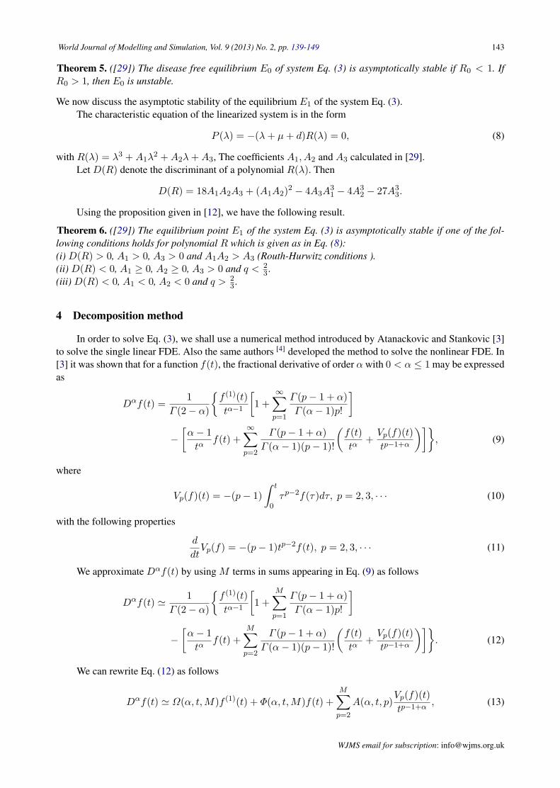
4 Decomposition method

In order to solve Eq. (3), we shall use a numerical method introduced by Atanackovic and Stankovic [3]to solve the single linear FDE. Also the same authors [4] developed the method to solve the nonlinear FDE. In[3] it was shown that for a function f(t), the fractional derivative of order α with 0 < α ≤ 1 may be expressedas

Dαf(t) =1

Γ (2− α)

f (1)(t)tα−1

[1 +

∞∑p=1

Γ (p− 1 + α)Γ (α− 1)p!

]

−[α− 1tα

f(t) +∞∑

p=2

Γ (p− 1 + α)Γ (α− 1)(p− 1)!

(f(t)tα

+Vp(f)(t)tp−1+α

)], (9)

where

Vp(f)(t) = −(p− 1)∫ t

0τp−2f(τ)dτ, p = 2, 3, · · · (10)

with the following properties

d

dtVp(f) = −(p− 1)tp−2f(t), p = 2, 3, · · · (11)

We approximate Dαf(t) by using M terms in sums appearing in Eq. (9) as follows

Dαf(t) ' 1Γ (2− α)

f (1)(t)tα−1

[1 +

M∑p=1

Γ (p− 1 + α)Γ (α− 1)p!

]

−[α− 1tα

f(t) +M∑

p=2

Γ (p− 1 + α)Γ (α− 1)(p− 1)!

(f(t)tα

+Vp(f)(t)tp−1+α

)]. (12)

We can rewrite Eq. (12) as follows

Dαf(t) ' Ω(α, t,M)f (1)(t) + Φ(α, t,M)f(t) +M∑

p=2

A(α, t, p)Vp(f)(t)tp−1+α

, (13)

WJMS email for subscription: info@wjms.org.uk

144 M. Javidi & N. Nyamorady: Numerical Behavior of a Fractional Order HIV/AIDS

where

Ω(α, t,M) =1 +

∑Mp=1

Γ (p−1+α)Γ (α−1)p!

Γ (2− α)tα−1, R(α, t) =

1− α

tαΓ (2− α),

A(α, t, p) = − Γ (p− 1 + α)Γ (2− α)Γ (α− 1)p!

, Φ(α, t,M) = R(α, t) +M∑

p=2

A(α, t, p)tα

.

We set

Θ1(t) = S(t), ΘM+1(t) = I(t),Θ2M+1(t) = J(t), Θp(t) = Vp(S)(t),Θ3M+1(t) = A(t), ΘM+p(t) = Vp(I)(t),Θ2M+p(t) = Vp(J)(t), Θ3M+p(t) = Vp(A)(t),

for p = 2, 3, · · · .We can rewrite system Eq.(3) as the following form

Ω(α, t,M)Θ′1(t) + Φ(α, t,M)Θ1(t) +

M∑p=2

A(α, t, p)Θp(t)tp−1+α

= µK − cβ(ΘM+1(t) + bΘ2M+1(t))Θ1(t)− µΘ1(t),

Ω(α, t,M)Θ′M+1(t) + Φ(α, t,M)ΘM+1(t) +

M∑p=2

A(α, t, p)ΘM+p(t)tp−1+α

= cβ(ΘM+1(t) + bΘ2M+1(t))Θ1(t)− (µ+ k1)ΘM+1(t) + αΘ2M+1(t),

Ω(α, t,M)Θ′2M+1(t) + Φ(α, t,M)Θ2M+1(t) +

M∑p=2

A(α, t, p)Θ2M+p(t)tp−1+α

= k1ΘM+1(t)− (µ+ k2 + α)Θ2M+1(t),

Ω(α, t,M)Θ′3M+1(t) + Φ(α, t,M)Θ3M+1(t) +

M∑p=2

A(α, t, p)Θ3M+p(t)tp−1+α

= k2Θ2M+1(t)− (µ+ d)Θ3M+1(t), (14)

where

Θp(t) = − (p− 1)∫ t

0τp−2Θ1(t)(τ)dτ,

ΘM+p(t) = − (p− 1)∫ t

0τp−2ΘM+1(t)(τ)dτ,

Θ2M+p(t) = − (p− 1)∫ t

0τp−2Θ2M+1(t)(τ)dτ,

Θ3M+p(t) = − (p− 1)∫ t

0τp−2Θ3M+1(t)(τ)dτ,

p = 2, 3, · · · ,M. (15)

Now we can rewrite Eq. (14) and Eq. (15) as the following form

WJMS email for contribution: submit@wjms.org.uk

World Journal of Modelling and Simulation, Vol. 9 (2013) No. 2, pp. 139-149 145

Θ′1(t) =

1Ω(α, t,M)

(µK − cβ(ΘM+1(t) + bΘ2M+1(t))Θ1(t)− µΘ1(t)

− Φ(α, t,M)Θ1(t)−M∑

p=2

A(α, t, p)Θp(t)tp−1+α

),

Θ′p(t) = − (p− 1)tp−2Θ1(t), p = 2, 3, · · · ,M,

Θ′M+1(t) =

1Ω(α, t,M)

(cβ(ΘM+1(t) + bΘ2M+1(t))Θ1(t)− (µ+ k1)ΘM+1(t)

+ αΘ2M+1(t)− Φ(α, t,M)ΘM+1(t)−M∑

p=2

A(α, t, p)ΘM+p(t)tp−1+α

),

Θ′M+p(t) = − (p− 1)tp−2ΘM+1(t), p = 2, 3, · · · ,M,

Θ′2M+1(t) =

1Ω(α, t,M)

(k1ΘM+1(t)− (µ+ k2 + α)Θ2M+1(t)

− Φ(α, t,M)Θ2M+1(t)−M∑

p=2

A(α, t, p)Θ2M+p(t)tp−1+α

),

Θ′2M+p(t) = − (p− 1)tp−2Θ2M+1(t), p = 2, 3, · · · ,M,

Θ′3M+1(t) =

1Ω(α, t,M)

(k2Θ2M+1(t)− (µ+ d)Θ3M+1(t)

− Φ(α, t,M)Θ2M+1(t)−M∑

p=2

A(α, t, p)Θ2M+p(t)tp−1+α

),

Θ′3M+p(t) = − (p− 1)tp−2Θ3M+1(t), p = 2, 3, · · · ,M, (16)

with the following initial conditions

Θ1(δ) = S0, Θp (δ) = 0, p = 2, 3, · · · ,M,

ΘM+1(δ) = I0, ΘM+p(δ) = 0, p = 2, 3, · · · ,M,

Θ2M+1(δ) = J0, Θ2M+p(δ) = 0, p = 2, 3, · · · ,M,

Θ3M+1(δ) = A0, Θ3M+p(δ) = 0, p = 2, 3, · · · ,M. (17)

No we consider the numerical solution of system of ordinary differential Eqs. (16) with the initial conditionsEq. (17) by using the well known Runge–Kutta method of order fourth.

5 Numerical methods and simulations

Now we solve the fractional order HIV/AIDS epidemic model in two cases.

Case 1. The parameters have been set to

K = 120, β = 0.0005, b = 0.3, µ = 0.02, c = 3, k1 = 0.01, k2 = 0.02, γ = 0.01, d = 0.02,

with the initial conditions

S0 = 100, I0 = 0.01, J0 = 160, A0 = 17.5.

andM = 10,∆t = 0.005.

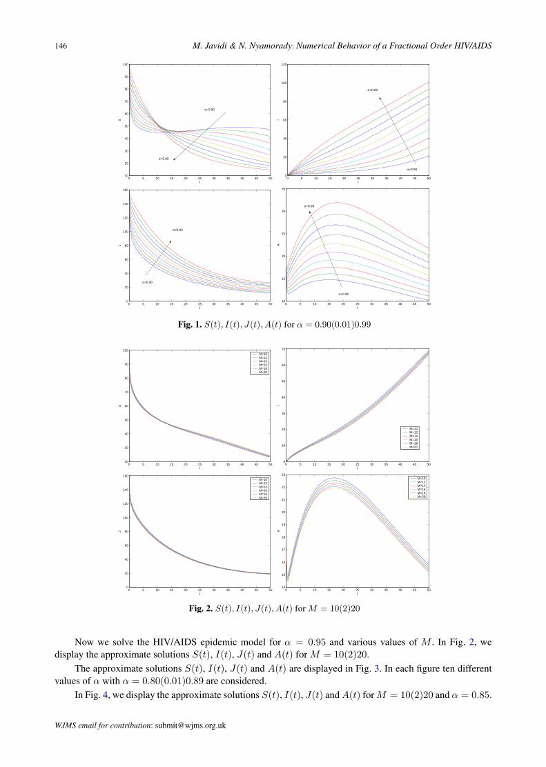
The approximate solutions S(t), I(t), J(t) and A(t) are displayed in Fig. 1. In each figure ten different valuesof α with α = 0.90(0.01)0.99 are considered.

WJMS email for subscription: info@wjms.org.uk

146 M. Javidi & N. Nyamorady: Numerical Behavior of a Fractional Order HIV/AIDSM. Javidi, N. Nyamorady 13

0 5 10 15 20 25 30 35 40 45 5010

20

30

40

50

60

70

80

90

100

t

S

α=0.90

α=0.99

0 5 10 15 20 25 30 35 40 45 500

20

40

60

80

100

120

t

I

α=0.90

α=0.99

0 5 10 15 20 25 30 35 40 45 500

20

40

60

80

100

120

140

160

t

J

α=0.90

α=0.99

0 5 10 15 20 25 30 35 40 45 5010

15

20

25

30

35

t

A

α=0.90

α=0.99

Figure 1: S(t), I(t), J(t), A(t) for α = 0.90(0.01)0.99

The approximate solutions S(t), I(t), J(t) and A(t) are displayed in Fig. 1. In each figure ten different values of α with

α = 0.90(0.01)0.99 are considered. Now we solve the HIV/AIDS epidemic model for α = 0.95 and various values of M .

In Fig. 2, we display the approximate solutions S(t), I(t), J(t) and A(t) for M = 10(2)20. The approximate solutions

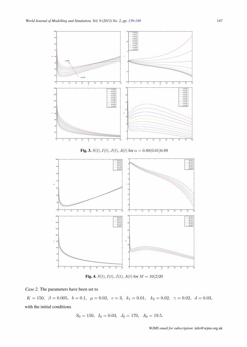
S(t), I(t), J(t) and A(t) are displayed in Fig. 3. In each figure ten different values of α with α = 0.80(0.01)0.89 are

considered. In Fig. 4, we display the approximate solutions S(t), I(t), J(t) and A(t) for M = 10(2)20 and α = 0.85.

Case II: The parameters have been set to

K = 150, β = 0.005, b = 0.1, µ = 0.02, c = 3, k1 = 0.01, k2 = 0.02, γ = 0.02, d = 0.03,

with the initial conditions

S0 = 150, I0 = 0.03, J0 = 170, A0 = 19.5.

and

M = 10, ∆t = 0.005.

WJMS homepage: http://www.wjms.org.uk/

Fig. 1. S(t), I(t), J(t), A(t) for α = 0.90(0.01)0.9914 World Journal of Modelling and Simulation,Vol.xx(20xx),No.xx,pp. 1-19

0 5 10 15 20 25 30 35 40 45 5020

30

40

50

60

70

80

90

100

t

S

M=10M=12M=14M=16M=18M=20

0 5 10 15 20 25 30 35 40 45 500

10

20

30

40

50

60

70

t

I

M=10M=12M=14M=16M=18M=20

0 5 10 15 20 25 30 35 40 45 500

20

40

60

80

100

120

140

160

t

J

M=10M=12M=14M=16M=18M=20

0 5 10 15 20 25 30 35 40 45 5014

15

16

17

18

19

20

21

22

23

t

A

M=10M=12M=14M=16M=18M=20

Figure 2: S(t), I(t), J(t), A(t) for M = 10(2)20

0 5 10 15 20 25 30 35 40 45 5020

30

40

50

60

70

80

90

100

t

S

α=0.80

α=0/89

0 5 10 15 20 25 30 35 40 45 50−10

−5

0

5

10

15

t

I

α=0.80α=0.81α=0.82α=0.83α=0.84α=0.85α=0.86α=0.87α=0.88α=0.89

0 5 10 15 20 25 30 35 40 45 500

20

40

60

80

100

120

140

160

t

J

α=0.80α=0.81α=0.82α=0.83α=0.84α=0.85α=0.86α=0.87α=0.88α=0.89

0 5 10 15 20 25 30 35 40 45 504

6

8

10

12

14

16

18

t

A

α=0.80α=0.81α=0.82α=0.83α=0.84α=0.85α=0.86α=0.87α=0.88α=0.89

Figure 3: S(t), I(t), J(t), A(t) for α = 0.80(0.01)0.89

WJMS email for contribution: editor@wjms.org.uk

Fig. 2. S(t), I(t), J(t), A(t) for M = 10(2)20

Now we solve the HIV/AIDS epidemic model for α = 0.95 and various values of M . In Fig. 2, wedisplay the approximate solutions S(t), I(t), J(t) and A(t) for M = 10(2)20.

The approximate solutions S(t), I(t), J(t) and A(t) are displayed in Fig. 3. In each figure ten differentvalues of α with α = 0.80(0.01)0.89 are considered.

In Fig. 4, we display the approximate solutions S(t), I(t), J(t) andA(t) forM = 10(2)20 and α = 0.85.

WJMS email for contribution: submit@wjms.org.uk

World Journal of Modelling and Simulation, Vol. 9 (2013) No. 2, pp. 139-149 147

14 World Journal of Modelling and Simulation,Vol.xx(20xx),No.xx,pp. 1-19

0 5 10 15 20 25 30 35 40 45 5020

30

40

50

60

70

80

90

100

t

S

M=10M=12M=14M=16M=18M=20

0 5 10 15 20 25 30 35 40 45 500

10

20

30

40

50

60

70

t

I

M=10M=12M=14M=16M=18M=20

0 5 10 15 20 25 30 35 40 45 500

20

40

60

80

100

120

140

160

t

J

M=10M=12M=14M=16M=18M=20

0 5 10 15 20 25 30 35 40 45 5014

15

16

17

18

19

20

21

22

23

t

A

M=10M=12M=14M=16M=18M=20

Figure 2: S(t), I(t), J(t), A(t) for M = 10(2)20

0 5 10 15 20 25 30 35 40 45 5020

30

40

50

60

70

80

90

100

t

S

α=0.80

α=0/89

0 5 10 15 20 25 30 35 40 45 50−10

−5

0

5

10

15

t

I

α=0.80α=0.81α=0.82α=0.83α=0.84α=0.85α=0.86α=0.87α=0.88α=0.89

0 5 10 15 20 25 30 35 40 45 500

20

40

60

80

100

120

140

160

t

J

α=0.80α=0.81α=0.82α=0.83α=0.84α=0.85α=0.86α=0.87α=0.88α=0.89

0 5 10 15 20 25 30 35 40 45 504

6

8

10

12

14

16

18

t

A

α=0.80α=0.81α=0.82α=0.83α=0.84α=0.85α=0.86α=0.87α=0.88α=0.89

Figure 3: S(t), I(t), J(t), A(t) for α = 0.80(0.01)0.89

WJMS email for contribution: editor@wjms.org.uk

Fig. 3. S(t), I(t), J(t), A(t) for α = 0.80(0.01)0.89M. Javidi, N. Nyamorady 15

0 5 10 15 20 25 30 35 40 45 5030

40

50

60

70

80

90

100

t

S

M=10M=12M=14M=16M=18M=20

0 5 10 15 20 25 30 35 40 45 50−9

−8

−7

−6

−5

−4

−3

−2

−1

0

1

t

I

M=10M=12M=14M=16M=18M=20

0 5 10 15 20 25 30 35 40 45 500

20

40

60

80

100

120

140

160

t

J

M=10M=12M=14M=16M=18M=20

0 5 10 15 20 25 30 35 40 45 504

6

8

10

12

14

16

18

t

A

M=10M=12M=14M=16M=18M=20

Figure 4: S(t), I(t), J(t), A(t) for M = 10(2)20

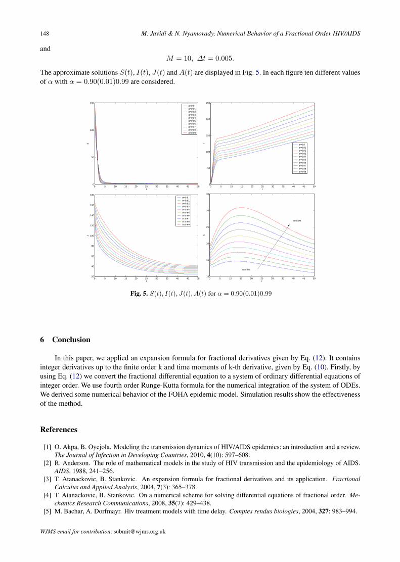
The approximate solutions S(t), I(t), J(t) and A(t) are displayed in Fig. 5. In each figure ten different values of α with

α = 0.90(0.01)0.99 are considered.

6 Conclusion

In this paper, we applied an expansion formula for fractional derivatives given by (12). It contains integer derivatives

up to the finite order k and time moments of k-th derivative, given by (10). Firstly, by using Eq. (12) we convert the

fractional differential equation to a system of ordinary differential equations of integer order. We use fourth order Runge-

Kutta formula for the numerical integration of the system of ODEs. We derived some numerical behavior of the FOHA

epidemic model. Simulation results show the effectiveness of the method.

WJMS homepage: http://www.wjms.org.uk/

Fig. 4. S(t), I(t), J(t), A(t) for M = 10(2)20

Case 2. The parameters have been set to

K = 150, β = 0.005, b = 0.1, µ = 0.02, c = 3, k1 = 0.01, k2 = 0.02, γ = 0.02, d = 0.03,

with the initial conditions

S0 = 150, I0 = 0.03, J0 = 170, A0 = 19.5.

WJMS email for subscription: info@wjms.org.uk

148 M. Javidi & N. Nyamorady: Numerical Behavior of a Fractional Order HIV/AIDS

andM = 10, ∆t = 0.005.

The approximate solutions S(t), I(t), J(t) and A(t) are displayed in Fig. 5. In each figure ten different valuesof α with α = 0.90(0.01)0.99 are considered.16 World Journal of Modelling and Simulation,Vol.xx(20xx),No.xx,pp. 1-19

0 5 10 15 20 25 30 35 40 45 500

50

100

150

t

S

α=0.9α=0.91α=0.92α=0.93α=0.94α=0.95α=0.96α=0.97α=0.98α=0.99

0 5 10 15 20 25 30 35 40 45 500

50

100

150

200

250

t

I α=0.9α=0.91α=0.92α=0.93α=0.94α=0.95α=0.96α=0.97α=0.98α=0.99

0 5 10 15 20 25 30 35 40 45 5020

40

60

80

100

120

140

160

180

t

J

α=0.9α=0.91α=0.92α=0.93α=0.94α=0.95α=0.96α=0.97α=0.98α=0.99

0 5 10 15 20 25 30 35 40 45 5010

15

20

25

30

35

t

A

α=0.90

α=0.99

Figure 5: S(t), I(t), J(t), A(t) for α = 0.90(0.01)0.99

References

[1] F. Nyabadza, Z. Mukandavire, S. D. Hove-Musekwa, Modelling the HIV/AIDS epidemic trends in South Africa:

Insights from a simple mathematical model, Nonlinear Analysis: Real World Applications, 12 (2011) 2091–2104.

[2] G. P. Samanta Permanence and extinction of a nonautonomous HIV/AIDS epidemic model with distributed time

delay, Nonlinear Analysis: Real World Applications, 12 (2011) 1163–1177.

[3] M. A. Yau and N. NO, An SIR mathematical model of HIV transmission dynamics , Applied Science Segment, 2(2)

APS/1551, 2011.

[4] M. A. Yau and N. NO, Epidemic mathematical model incorporating complacency as a measure of control, Applied

Science Segment, 2(2) APS/1556, 2011.

[5] W. Zunyou, R. Keming, C. Haixia The HIV/AIDS Epidemic in China: History, Current Strategies and Future

Challenges, AIDS Education and Prevention, 16 (2004) 7–17. (2004).

[6] H. W. Hethcote and A. J. Van Modeling HIV Transmission and AIDS in the United States, Lecture notes in Biomath-

ematics 95. Springer-Verlag, New York, 234 p. (1992).

WJMS email for contribution: editor@wjms.org.uk

Fig. 5. S(t), I(t), J(t), A(t) for α = 0.90(0.01)0.99

6 Conclusion

In this paper, we applied an expansion formula for fractional derivatives given by Eq. (12). It containsinteger derivatives up to the finite order k and time moments of k-th derivative, given by Eq. (10). Firstly, byusing Eq. (12) we convert the fractional differential equation to a system of ordinary differential equations ofinteger order. We use fourth order Runge-Kutta formula for the numerical integration of the system of ODEs.We derived some numerical behavior of the FOHA epidemic model. Simulation results show the effectivenessof the method.

References

[1] O. Akpa, B. Oyejola. Modeling the transmission dynamics of HIV/AIDS epidemics: an introduction and a review.The Journal of Infection in Developing Countries, 2010, 4(10): 597–608.

[2] R. Anderson. The role of mathematical models in the study of HIV transmission and the epidemiology of AIDS.AIDS, 1988, 241–256.

[3] T. Atanackovic, B. Stankovic. An expansion formula for fractional derivatives and its application. FractionalCalculus and Applied Analysis, 2004, 7(3): 365–378.

[4] T. Atanackovic, B. Stankovic. On a numerical scheme for solving differential equations of fractional order. Me-chanics Research Communications, 2008, 35(7): 429–438.

[5] M. Bachar, A. Dorfmayr. Hiv treatment models with time delay. Comptes rendus biologies, 2004, 327: 983–994.

WJMS email for contribution: submit@wjms.org.uk

World Journal of Modelling and Simulation, Vol. 9 (2013) No. 2, pp. 139-149 149

[6] R. Bagley, R. Calico. Fractional order state equations for the control of viscoelastically damped structures. Journalof Guidance, Control, and Dynamics, 1991, 14: 304–311.

[7] S. Blower. Calculating the consequences: Haart and risky sex. AIDS, 2001, 15: 1309–1310.[8] D. Kusnezov, A. Bulgac, G. Dang. Quantum levy processes and fractional kinetics. Physical review letters, 1999,

2: 1136–1139.[9] K. Diethelm, N. Ford. Analysis of fractional differential equations. Journal of Mathematical Analysis and Appli-

cations, 2002, 265: 229–248.[10] K. Diethelm, N. Ford. Multi-order fractional differential equations and their numerical solution. Applied Mathe-

matics and Computation, 2004, 154: 621–640.[11] P. Driessche, J. Watmough. Reproduction numbers and sub-threshold endemic equilibria for compartmental models

of disease transmission. Mathematical biosciences, 2002, 180: 29–48.[12] E. Ahmed, A. El-Sayed, H. El-Saka. On some routh-hurwitz conditions for fractional order differential equations

and their applications in lorenz, rossler, chua and chen systems. Physics Letters A, 2006, 258: 1–4.[13] F. Nyabadza, Z. Mukandavire, S. Hove-Musekwa. Modelling the HIV/AIDS epidemic trends in south africa:

Insights from a simple mathematical model. Nonlinear Analysis: Real World Applications, 2011, 12: 2091–2104.[14] S. Samko, A. Kilbas, O. Marichev. Fractional integrals and derivatives: Theory and applications. Gordon and

Breach, Amsterdam, 1993.[15] H. Hethcote, J. Van Ark. Modelling HIV Transmission and AIDS in the United States. Springer, Berlin, 1992.[16] H. Hethcote, A. Van. Modeling HIV Transmission and AIDS in the United States. Springer-Verlag, New York,

1992. Lecture notes in Biomathematics 95.[17] R. Hilfer. Applications of fractional calculus in physics. New Jersey: World Scientific, 2001.[18] K. Diethelm, N. Ford, A. Freed. Detailed error analysis for a fractional adams method. Numerical algorithms,

2004, 36: 31–52.[19] V. Lakshmikantham, A. Vatsala. Basic theory of fractional differential equations. Nonlinear Analysis: Theory,

Methods & Applications, 2008, 69(8): 2677–2682.[20] N. Laskin. Fractals and quantum mechanics. Chaos: An Interdisciplinary Journal of Nonlinear Science, 2000, 10:

780–790.[21] N. Laskin. Fractional market dynamics. Physica A: Statistical Mechanics and its Applications, 2000, 287: 482–492.[22] N. Laskin. Fractional quantum mechanics. Physical Review E, 2000, 62: 3135–3145.[23] N. Laskin. Fractional quantum mechanics and levy path integrals. Physics Letters A, 2000, 298: 298–305.[24] N. Laskin. Fractional schrdinger equation. Physical Review E, 2002, 66: 56–108.[25] W. Lin. Global existence theory and chaos control of fractional differential equations. Journal of Mathematical

Analysis and Appications, 2007, 332: 709–726.[26] M. Ichise, Y. Nagayanagi, T. Kojima. An analog simulation of non-integer order transfer functions for analysis of

electrode process. Journal of Electroanalytical Chemistry, 1971, 33: 253–265.[27] D. Matignon. Stability result on fractional differential equations with applications to control processing. Compu-

tational engineering in systems applications, 1996, 963–968.[28] C. McCluskey. A model of HIV/AIDS with staged progression and amelioration. Mathematical biosciences, 2003,

181: 1–16.[29] N. Nyamorady, M. Javidi. A fractional order HIV/AIDS epidemic model with treatment. SIAM review.[30] A. Perelson, P. Nelson. Mathematical analysis of HIV-1 dynamics in vivo. SIAM review, 1999, 41: 3–44.[31] I. Podlubny. Fractional Differential Equations. Academic Press, New York, 1999.[32] R. Agarwal, M. Benchohra, S. Hamani. A survey on existence results for boundary value problems of nonlinear

fractional differential equations and inclusions. Acta Applicandae Mathematicae, 2010, 109: 973–1033.[33] R. Anderson, C. Medley, et al. A preliminary study of the transmission dynamics of the human immunodeficiency

virus (HIV), the causative agent of AIDS. Mathematical Medicine and Biology, 1986, 3: 229–263.[34] G. Samanta. Permanence and extinction of a nonautonomous HIV/AIDS epidemic model with distributed time

delay. Nonlinear Analysis: Real World Applications, 2011, 12: 1163–1177.[35] C. Stoddart, R. Reyes. Models of HIV-1 disease: A review of current status, drug discovery today. Disease, 2006,

3(1): 113–119.[36] Z. Wu, K. Rou, H. Cui. The HIV/AIDS epidemic in China: History, current strategies and future challenges. AIDS

Education and Prevention, 2004, 16: 7–17.[37] T. Wan-Yuan. Stochastic Modeling of AIDS Epidemiology and HIV Pathogenesis. World Scientific Publishing,

Singapore, 2000.[38] M. Yau, N. NO. Epidemic mathematical model incorporating complacency as a measure of control. Applied

Science Segment, 2011, 2(2): APS/1556.[39] M. Yau, N. NO. An sir mathematical model of HIV transmission dynamics. Applied Science Segment, 2011, 2(2):

APS/1551.

WJMS email for subscription: info@wjms.org.uk