Modelling of aqueous electrolyte solutions with theSAFT γ−Mie framework

Ana Patrıcia Cardoso Cotrim

Thesis to obtain the Master of Science Degree in

Chemical Engineering

Advisor(s)/Supervisor(s): Dr. Thomas LafitteDr. Pedro Jorge Rodrigues Morgado

Examination CommitteeChairperson:

Advisor:Members of the Committee:

Prof./Dr. Carlos HenriquesProf./Dr. Pedro MorgadoProf./Dr. Eduardo Filipe

November 2018

Acknowledgements

This thesis is not the result of merely a single person’s effort. In the first place, I would like to extendmy sincere gratitude to Professor Costas Pantelides for the opportunity to work at Process SystemsEnterprise. A special acknowledgement goes to Professor Eduardo Filipe, for all his invaluable supportand, again, for the opportunity to make this internship possible. I would especially like to thank mysupervisor, Dr. Pedro Morgado, for all his help at every stage.

To all the gSAFT team, who were always willing to help whenever necessary. To my supervisor, Dr.Thomas Laffite, it was a pleasure to work with you and learn from you. Furthermore, I cannot find thewords to express my gratitude to Dr. Simon Dufal and Dr. Vasileios Papaioannou who followed thisproject from the beginning, advising and supporting me during all this experience. Without them, thisthesis would have been much more difficult to accomplish.

To my friends and my housemates: Alexandre, Diogo and Mauro, who were my family here. Theexperiences and moments we shared will always be remembered with affection. To Renato, Artur, Tomand Andre for hosting us in our first days in London, and to all the other Portuguese people present inLondon: Mariana, Francisco, Joao, Beatriz and Joao Barras. We were extremely fortunate to have suchnice people here with us.

To my family and to Jose, for always believing in me as well as advising and supporting me in everymoment of my life. I will be forever in great debt to you and I will always remember your endless loveand encouragement.

i

Abstract

This thesis is based on a study of the thermodynamic properties of electrolyte solutions. The purposeof this work is to understand which combination of experimental data should be used to develop theSAFT γ-Mie model parameters for electrolytes. In order to carry out this study, the approach that is usedis based on studying first four different salts (NaCl, NaBr, KCl and KBr) and then applying what isbelieved to be the best estimation strategy to other salts such as NaI, KI, RbCl, RbBr, CsCl, CsBr,NaNO3, KNO3, NH4Cl and NH4Br.

The obtained results are based on the computation of a broad set of properties such as solubilities,liquid phase densities, liquid phase heat capacities and heats of dilution. One of the important conclu-sions taken from this work is the importance of including calorific properties (heat capacities and heatsof dilution) when developing model parameters for electrolytes.

Keywords: SAFT, gSAFT, Modelling, Electrolyte Solutions, Salt Based Solutions, Solubility, LiquidPhase Density, Liquid phase Heat Capacities, Dilution Enthalpy, Mean Activity Coefficients, OsmoticCoefficients

iii

Resumo

Esta tese baseia-se num estudo das propriedades termodinamicas de solucoes de eletrolitos. Oobjetivo deste trabalho e perceber qual a combinacao de dados experimentais que deve ser utilizadapara desenvolver os parametros do modelo de SAFT γ-Mie para eletrolitos. De modo a prosseguircom este estudo a estrategia que e usada e baseada em estudar primeiro quatro sais distintos (NaCl,NaBr, KCl and KBr) e depois em aplicar aquela que se cre ser a melhor estrategia de estimativas aoutros sais, tais como NaI, KI, RbCl, RbBr, CsCl, CsBr, NaNO3, KNO3, NH4Cl and NH4Br.

Os resultados obtidos sao baseados na computacao de um conjunto amplo de propriedades taiscomo solubilidades, densidades da fase lıquida, capacidades calorıficas e entalpias de dissolucao. Umadas conclusoes importantes que se reteve deste trabalho e a importancia de se incluirem propriedadescalorıficas (capacidades calorıficas e entalpias de diluicao) aquando o desenvolvimento de parametrosdo modelo para eletrolitos.

Keywords: SAFT, gSAFT, Modelacao, Solucoes de eletrolitos, Solucoes de sais, Solubilidade,Densidade da fase lıquida, Capacidades calorıficas da fase lıquida, Entalpia de diluicao, Coeficientesde Atividade, Coeficientes Osmoticos.

v

Contents

List of Tables viii

List of Figures x

Nomenclature xv

1 Introduction 1

2 State of the Art 32.1 Thermodynamic modelling of electrolyte-containing systems . . . . . . . . . . . . . . . . . 3

2.1.1 Primitive and non-primitive models . . . . . . . . . . . . . . . . . . . . . . . . . . . 32.2 Published works . . . . . . . . . . . . . . . . . . . . . . . . . . . . . . . . . . . . . . . . . 4

3 Thermodynamic fundamentals for solubility calculation 53.1 Liquid Phase Chemical Potential . . . . . . . . . . . . . . . . . . . . . . . . . . . . . . . . 63.2 Solid Phase Chemical Potential . . . . . . . . . . . . . . . . . . . . . . . . . . . . . . . . . 7

4 SAFT γ - Mie Equation of State 94.1 Evolution of Equations of State . . . . . . . . . . . . . . . . . . . . . . . . . . . . . . . . . 94.2 Molecular model and intermolecular potential . . . . . . . . . . . . . . . . . . . . . . . . . 94.3 SAFT γ - Mie: free energy contributions . . . . . . . . . . . . . . . . . . . . . . . . . . . . 11

4.3.1 Ideal term . . . . . . . . . . . . . . . . . . . . . . . . . . . . . . . . . . . . . . . . . 124.3.2 Monomer term . . . . . . . . . . . . . . . . . . . . . . . . . . . . . . . . . . . . . . 134.3.3 Chain term . . . . . . . . . . . . . . . . . . . . . . . . . . . . . . . . . . . . . . . . 144.3.4 Association term . . . . . . . . . . . . . . . . . . . . . . . . . . . . . . . . . . . . . 144.3.5 Born Contribution . . . . . . . . . . . . . . . . . . . . . . . . . . . . . . . . . . . . 144.3.6 MSA Contribution . . . . . . . . . . . . . . . . . . . . . . . . . . . . . . . . . . . . 15

5 Development of model parameters and analyses of the systems of interest 175.1 Description of parameters . . . . . . . . . . . . . . . . . . . . . . . . . . . . . . . . . . . . 175.2 Experimental Data . . . . . . . . . . . . . . . . . . . . . . . . . . . . . . . . . . . . . . . . 185.3 Systems of interest . . . . . . . . . . . . . . . . . . . . . . . . . . . . . . . . . . . . . . . . 19

6 Parameter Estimation Strategy and Results 216.1 Estimation using solubility . . . . . . . . . . . . . . . . . . . . . . . . . . . . . . . . . . . . 216.2 Estimation using solubility and liquid phase density . . . . . . . . . . . . . . . . . . . . . . 226.3 Estimation using solubility, liquid phase density and heat capacity . . . . . . . . . . . . . . 256.4 Estimation using solubility, liquid phase density and heat capacity and Dilution enthalpy . 296.5 Remarks . . . . . . . . . . . . . . . . . . . . . . . . . . . . . . . . . . . . . . . . . . . . . 33

vii

6.6 Extension to other salts . . . . . . . . . . . . . . . . . . . . . . . . . . . . . . . . . . . . . 35

7 Conclusions 41

Bibliography 42

A Fitting solid phase properties 45A.1 Predicting Solid Heat Capacities with solubility data . . . . . . . . . . . . . . . . . . . . . 45

B Gibbs Energy of Solvation 47

C Parameter Estimation Results 49C.1 Estimation using solubility . . . . . . . . . . . . . . . . . . . . . . . . . . . . . . . . . . . . 49

C.1.1 Liquid Phase Density results . . . . . . . . . . . . . . . . . . . . . . . . . . . . . . 49C.1.2 Liquid Phase Heat Capacity results . . . . . . . . . . . . . . . . . . . . . . . . . . 50C.1.3 Dilution Enthalpy results . . . . . . . . . . . . . . . . . . . . . . . . . . . . . . . . . 51C.1.4 Mean activity coefficient results . . . . . . . . . . . . . . . . . . . . . . . . . . . . . 52C.1.5 Osmotic Coefficient results . . . . . . . . . . . . . . . . . . . . . . . . . . . . . . . 53

C.2 Estimation using Solubility and Liquid Phase Density . . . . . . . . . . . . . . . . . . . . . 55C.2.1 First Attempt . . . . . . . . . . . . . . . . . . . . . . . . . . . . . . . . . . . . . . . 55

Liquid Phase Density results . . . . . . . . . . . . . . . . . . . . . . . . . . . . . . 56Mean Activity Coefficient results . . . . . . . . . . . . . . . . . . . . . . . . . . . . 59Osmotic Coefficients results . . . . . . . . . . . . . . . . . . . . . . . . . . . . . . . 60

C.2.2 Second Attempt . . . . . . . . . . . . . . . . . . . . . . . . . . . . . . . . . . . . . 61Liquid Phase Heat Capacity results . . . . . . . . . . . . . . . . . . . . . . . . . . 61Dilution Enthalpy results . . . . . . . . . . . . . . . . . . . . . . . . . . . . . . . . . 62Osmotic Coefficients results . . . . . . . . . . . . . . . . . . . . . . . . . . . . . . . 64

C.3 Estimation using solubility, liquid phase density and heat capacity . . . . . . . . . . . . . . 66C.3.1 First Attempt . . . . . . . . . . . . . . . . . . . . . . . . . . . . . . . . . . . . . . . 66

Liquid Phase Density results . . . . . . . . . . . . . . . . . . . . . . . . . . . . . . 67Dilution Enthalpy results . . . . . . . . . . . . . . . . . . . . . . . . . . . . . . . . . 69Mean Activity Coefficient results . . . . . . . . . . . . . . . . . . . . . . . . . . . . 70Osmotic Coefficient results . . . . . . . . . . . . . . . . . . . . . . . . . . . . . . . 71

C.3.2 Second Attempt . . . . . . . . . . . . . . . . . . . . . . . . . . . . . . . . . . . . . 72Dilution enthalpy results . . . . . . . . . . . . . . . . . . . . . . . . . . . . . . . . . 72Mean Activity Coefficients . . . . . . . . . . . . . . . . . . . . . . . . . . . . . . . . 73Osmotic Coefficient results . . . . . . . . . . . . . . . . . . . . . . . . . . . . . . . 74

C.4 Estimation using solubility, liquid phase density, liquid phase heat capacity and dilutionenthalpy . . . . . . . . . . . . . . . . . . . . . . . . . . . . . . . . . . . . . . . . . . . . . . 76C.4.1 Mean Activity Coefficients results . . . . . . . . . . . . . . . . . . . . . . . . . . . . 76C.4.2 Osmotic Coefficient results . . . . . . . . . . . . . . . . . . . . . . . . . . . . . . . 77

C.5 Model Extension . . . . . . . . . . . . . . . . . . . . . . . . . . . . . . . . . . . . . . . . . 78C.5.1 Mean Activity Coefficients results . . . . . . . . . . . . . . . . . . . . . . . . . . . . 78C.5.2 Osmotic Coefficients results . . . . . . . . . . . . . . . . . . . . . . . . . . . . . . . 79

viii

List of Tables

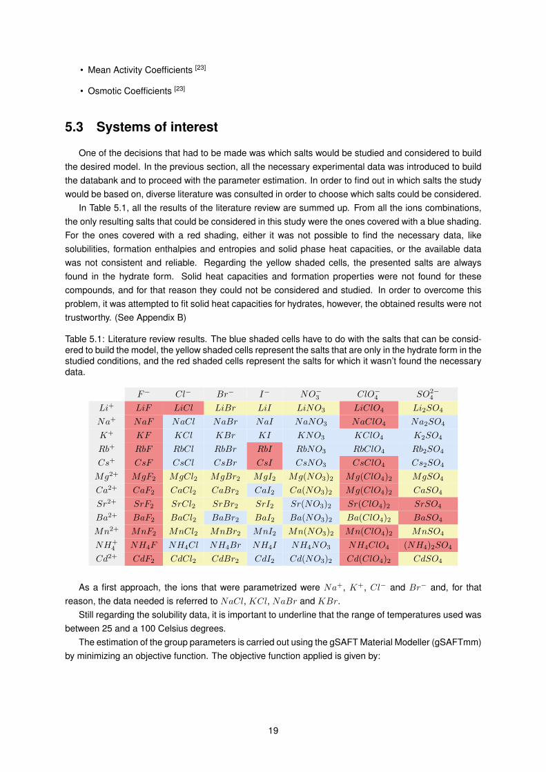
5.1 Literature review results. The blue shaded cells have to do with the salts that can beconsidered to build the model, the yellow shaded cells represent the salts that are only inthe hydrate form in the studied conditions, and the red shaded cells represent the saltsfor which it wasn’t found the necessary data. . . . . . . . . . . . . . . . . . . . . . . . . . 19

6.1 Comparison of solubility results for NaCl and corresponding %∆. . . . . . . . . . . . . . 23

6.2 Sigma values for the model with solubilities, liquid phase densities, liquid phase heatcapacities and dilution enthalpies. Values of ionic σ for the different ions. . . . . . . . . . . 33

6.3 Parameter Estimation Values for the model with solubilities, liquid phase densities, liquidphase heat capacities and dilution enthalpies. Values of ε for the different ions interactions. 34

6.4 Fitted properties and obtained results for Solubilities, Liquid phase densities, Mean Activ-ity Coefficients, Liquid phase heat capacities, dilution enthalpies and osmotic coefficients.The X is for the correct values, the × for incorrect values and the ± for results that arenot completely correct. . . . . . . . . . . . . . . . . . . . . . . . . . . . . . . . . . . . . . . 34

6.5 Adjustable parameters that were fitted in each approach. . . . . . . . . . . . . . . . . . . 34

6.6 Summary and the order in which the salts were studied. . . . . . . . . . . . . . . . . . . . 35

B.1 Gibbs energy of solvation ∆Gs of the ions studied: experimental values of Fawcett[25] andSAFT calculations. . . . . . . . . . . . . . . . . . . . . . . . . . . . . . . . . . . . . . . . . 47

C.1 Obtained parameters when only fitting to solubilities. Values of ionic σ for the different ions. 53

C.2 Obtained parameters when only fitting to solubilities. Values of ε for the different ionsinteractions. . . . . . . . . . . . . . . . . . . . . . . . . . . . . . . . . . . . . . . . . . . . . 54

C.3 Obtained parameters when fitting to solubilities and liquid phase densities. Values of ionicσ for the different ions. . . . . . . . . . . . . . . . . . . . . . . . . . . . . . . . . . . . . . . 64

C.4 Obtained parameters when fitting to solubilities and liquid phase densities. Values of ε forthe different ions interactions. . . . . . . . . . . . . . . . . . . . . . . . . . . . . . . . . . . 65

C.5 Obtained parameters when fitting to solubilities, liquid phase densities and liquid phaseheat capacities. Values of ionic σ for the different ions. . . . . . . . . . . . . . . . . . . . . 74

C.6 Obtained parameters when fitting to solubilities, liquid phase densities and liquid phaseheat capacities. Values of ε for the different ions interactions. . . . . . . . . . . . . . . . . 75

C.7 Obtained parameters for the final models. Values of ionic σ for the different ions. . . . . . 79

C.8 Obtained parameters for the RbCl and RbBr final model. Values of ε for the different ionsinteractions. . . . . . . . . . . . . . . . . . . . . . . . . . . . . . . . . . . . . . . . . . . . . 80

C.9 Obtained parameters for the CsCl and CsBr final model. Values of ε for the different ionsinteractions. . . . . . . . . . . . . . . . . . . . . . . . . . . . . . . . . . . . . . . . . . . . . 80

C.10 Obtained parameters for the NH4Cl and NH4Br final model. Values of ε for the differentions interactions. . . . . . . . . . . . . . . . . . . . . . . . . . . . . . . . . . . . . . . . . . 80

ix

C.11 Obtained parameters for the NaI and KI final model. Values of ε for the different ionsinteractions. . . . . . . . . . . . . . . . . . . . . . . . . . . . . . . . . . . . . . . . . . . . . 80

C.12 Obtained parameters for the NaNO3 and KNO3 final model. Values of ε for the differentions interactions. . . . . . . . . . . . . . . . . . . . . . . . . . . . . . . . . . . . . . . . . . 80

x

List of Figures

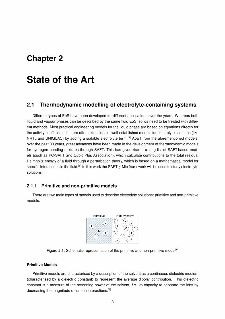
2.1 Schematic representation of the primitive and non-primitive model[6] . . . . . . . . . . . . 3

3.1 Summary of the various possible thermodynamic paths for the computation of chemi-cal potential of compound i in liquid phases µli(T, P, n) from the various standard stateformation properties, ideal gas, pure liquid, and “infinite dilution”. The thermodynamic in-tegration path depends on whether an equation of state (EoS) or activity coefficient model(ACM) is used to model the mixture non-idealities.[9] . . . . . . . . . . . . . . . . . . . . . 7

4.1 SAFT γ - Mie group contribution representation[11] . . . . . . . . . . . . . . . . . . . . . . 10

4.2 Mie potential representation in function of the distance between two particles . . . . . . . 11

4.3 Schematic representation of the different free energy contributions. The darker back-ground represents the dielectric medium.[4] . . . . . . . . . . . . . . . . . . . . . . . . . . 12

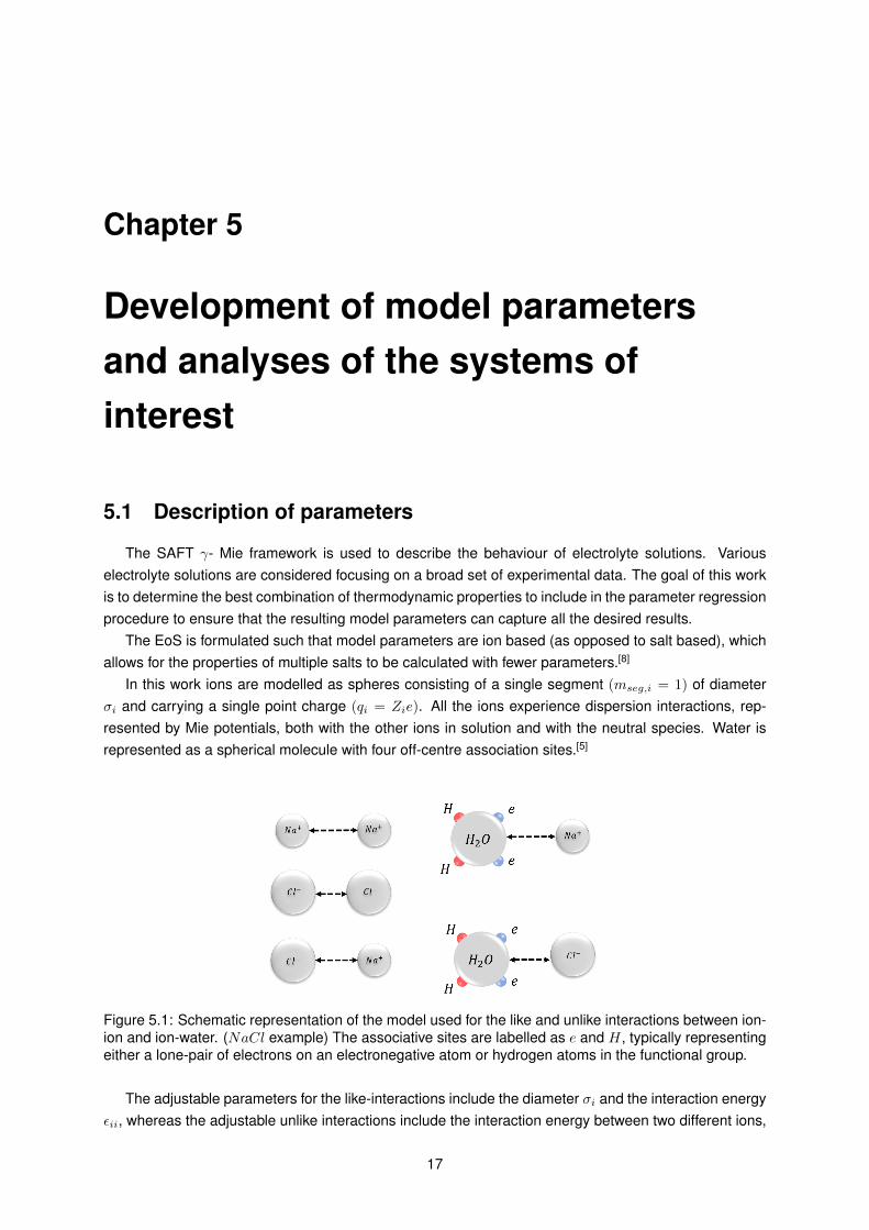
5.1 Schematic representation of the model used for the like and unlike interactions betweenion-ion and ion-water. (NaCl example) The associative sites are labelled as e and H, typ-ically representing either a lone-pair of electrons on an electronegative atom or hydrogenatoms in the functional group. . . . . . . . . . . . . . . . . . . . . . . . . . . . . . . . . . . 17

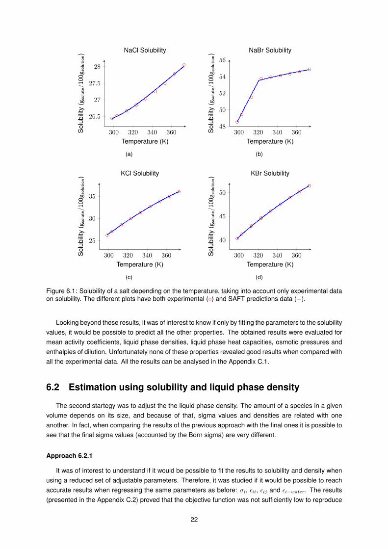
6.1 Solubility of a salt depending on the temperature, taking into account only experimentaldata on solubility. The different plots have both experimental () and SAFT predictionsdata (−). . . . . . . . . . . . . . . . . . . . . . . . . . . . . . . . . . . . . . . . . . . . . . . 22

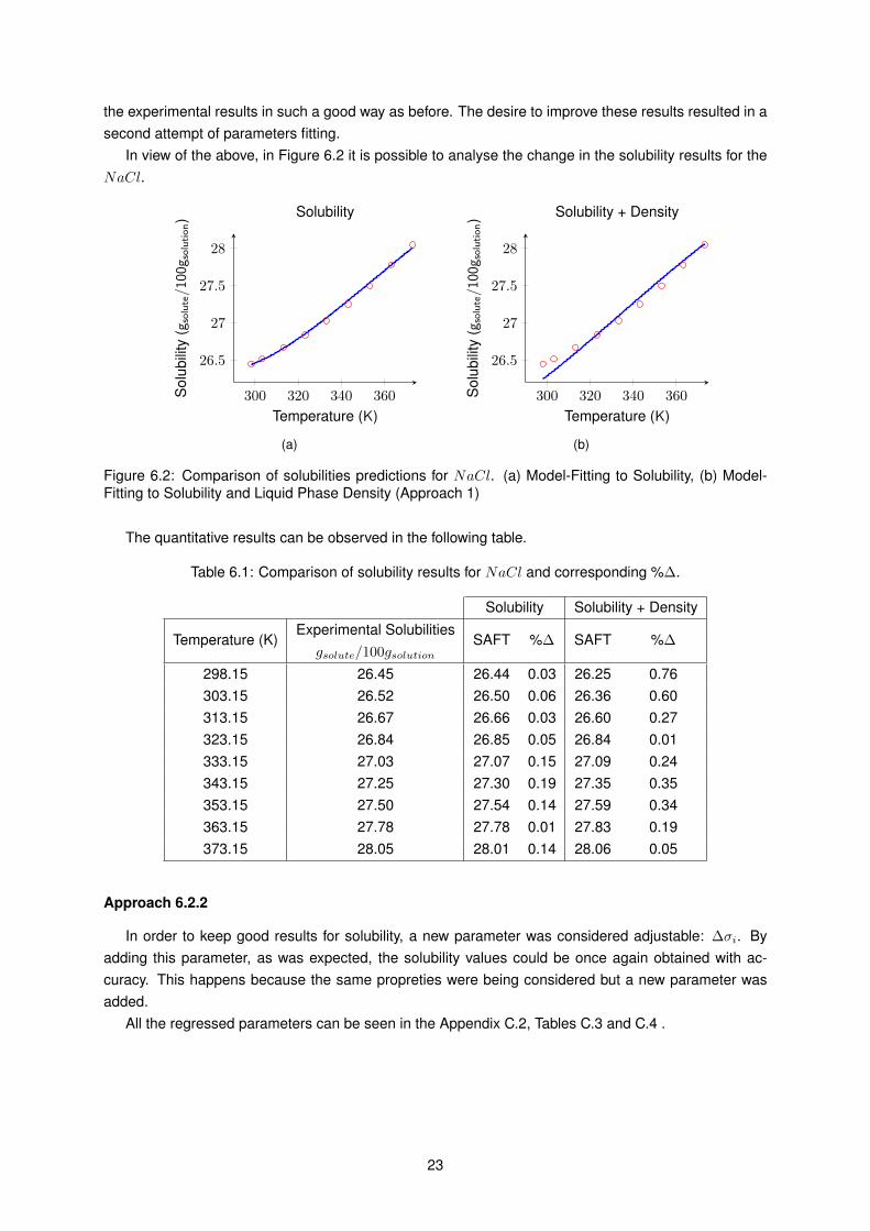
6.2 Comparison of solubilities predictions for NaCl. (a) Model-Fitting to Solubility, (b) Model-Fitting to Solubility and Liquid Phase Density (Approach 1) . . . . . . . . . . . . . . . . . 23

6.3 Solubility of a salt depending on the temperature, taking into account experimental dataon solubility and liquid phase densities. The different plots have both experimental () andSAFT predictions data (−). . . . . . . . . . . . . . . . . . . . . . . . . . . . . . . . . . . . 24

6.4 Liquid phase densities results, taking into account experimental data on solubility and liq-uid phase densities. The different plots have both experimental () and SAFT predictionsdata (−). . . . . . . . . . . . . . . . . . . . . . . . . . . . . . . . . . . . . . . . . . . . . . . 25

6.5 Comparison of solubilities results for NaCl. (a) Model-Fitting to Solubility + Liquid PhaseDensity, (b) Model-Fitting to Solubility + Liquid Phase Density + Liquid phase heat capac-ities(First Attempt) . . . . . . . . . . . . . . . . . . . . . . . . . . . . . . . . . . . . . . . . 26

6.6 Solubility of a salt depending on the temperature, taking into account experimental dataon solubility, liquid phase densities and liquid phase heat capacities. The different plotshave both experimental () and SAFT predictions data (−). . . . . . . . . . . . . . . . . . 27

6.7 Liquid phase density depending on the molality, taking into account experimental data onsolubility, liquid phase densities and liquid phase heat capacities. The different plots haveboth experimental () and SAFT predictions data (−). . . . . . . . . . . . . . . . . . . . . 28

xi

6.8 Liquid phase heat capacity of a salt depending on the molality, taking into account ex-perimental data on solubility, liquid phase density and liquid phase heat capacities. Thedifferent plots have both experimental () and SAFT predictions data (−). . . . . . . . . . 29

6.9 Solubility of a salt depending on the temperature, taking into account experimental dataon solubility, liquid phase densities, liquid phase heat capacities and dilution enthalpies.The different plots have both experimental () and SAFT predictions data (−). . . . . . . . 30

6.10 Liquid Phase Densities depending on molality, taking into account experimental data onsolubility, liquid phase densities, liquid phase heat capacities and dilution enthalpies. Thedifferent plots have both experimental () and SAFT predictions data (−). . . . . . . . . . 31

6.11 Liquid phase heat capacity of a salt depending on the molality, taking into account exper-imental data on solubility, liquid phase density, liquid phase heat capacities and dilutionenthalpy. The different plots have both experimental () and SAFT predictions data (−). . 32

6.12 Dilution enthalpy of a salt depending on the molality, taking into account experimental dataon solubility, liquid phase density, liquid phase heat capacity and dilution enthalpy. Thedifferent plots have both experimental () and SAFT predictions data (−). . . . . . . . . . 33

6.13 Solubility predictions for other compounds with an extension of the previous model. Themodel results are represented by the continuous line and the experimental points by thecircular marks. . . . . . . . . . . . . . . . . . . . . . . . . . . . . . . . . . . . . . . . . . . 36

6.14 Liquid phase densities predictions for other compounds with an extension of the previousmodel. The model results are represented by the continuous line and the experimentalpoints by the circular marks. . . . . . . . . . . . . . . . . . . . . . . . . . . . . . . . . . . . 37

6.15 Liquid phase heat capacities predictions for other compounds with an extension of theprevious model. The model results are represented by the continuous line and the exper-imental points by the circular marks. . . . . . . . . . . . . . . . . . . . . . . . . . . . . . . 38

6.16 Dilution Enthalpies predictions for other compounds with an extension of the previousmodel. The model results are represented by the continuous line and the experimentalpoints by the circular marks. . . . . . . . . . . . . . . . . . . . . . . . . . . . . . . . . . . . 39

A.1 Solubility predictions for MgCl2 · 6 H2O when fitting the solid heat capacity coefficients.The experimental data is represented by () and SAFT predictions by (−) . . . . . . . . . 46

A.2 Solid phase heat capacity predictions for MgCl2 · 6 H2O when fitting the solid heat capacitycoefficients to solubility values. The experimental data is represented by () and SAFTpredictions by (−) . . . . . . . . . . . . . . . . . . . . . . . . . . . . . . . . . . . . . . . . 46

C.1 Liquid phase density depending on the molality, taking into account only experimentaldata on solubility. The different plots have both experimental () and SAFT predictionsdata (−). . . . . . . . . . . . . . . . . . . . . . . . . . . . . . . . . . . . . . . . . . . . . . . 49

C.2 Liquid phase heat capacity of a salt depending on the molality, taking into account onlyexperimental data on solubility. The different plots have both experimental () and SAFTpredictions data (−). . . . . . . . . . . . . . . . . . . . . . . . . . . . . . . . . . . . . . . . 50

C.3 Dilution enthalpy of a salt depending on the molality, taking into account only experimentaldata on solubility. The different plots have both experimental () and SAFT predictionsdata (−). . . . . . . . . . . . . . . . . . . . . . . . . . . . . . . . . . . . . . . . . . . . . . . 51

C.4 Mean activity coefficient of a salt depending on the molality, taking into account onlyexperimental data on solubility. The different plots have both experimental () and SAFTpredictions data (−). . . . . . . . . . . . . . . . . . . . . . . . . . . . . . . . . . . . . . . . 52

xii

C.5 Osmotic coefficients of a salt depending on the molality, taking into account only experi-mental data on solubility. The different plots have both experimental () and SAFT predic-tions data (−). . . . . . . . . . . . . . . . . . . . . . . . . . . . . . . . . . . . . . . . . . . 53

C.6 Solubility of a salt depending on the temperature, taking into account only experimentaldata on solubility and liquid phase densities. The different plots have both experimental() and SAFT predictions data (−). . . . . . . . . . . . . . . . . . . . . . . . . . . . . . . . 55

C.7 Liquid phase density depending on the molality, taking into account only experimentaldata on solubility and liquid phase densities. The different plots have both experimental() and SAFT predictions data (−). . . . . . . . . . . . . . . . . . . . . . . . . . . . . . . . 56

C.8 Liquid phase heat capacity of a salt depending on the molality, taking into account exper-imental data on solubility and liquid phase density. The different plots have both experi-mental () and SAFT predictions data (−). . . . . . . . . . . . . . . . . . . . . . . . . . . . 57

C.9 Dilution enthalpy of a salt depending on the molality, taking into account experimental dataon solubility and liquid phase density. The different plots have both experimental () andSAFT predictions data (−). . . . . . . . . . . . . . . . . . . . . . . . . . . . . . . . . . . . 58

C.10 Mean activity coefficient of a salt depending on the molality, taking only into accountexperimental data on solubility and liquid phase densities. The different plots have bothexperimental () and SAFT predictions data (−). . . . . . . . . . . . . . . . . . . . . . . . 59

C.11 Osmotic coefficients of a salt depending on the molality, taking only into account experi-mental data on solubility and liquid phase densities. The different plots have both experi-mental () and SAFT predictions data (−). . . . . . . . . . . . . . . . . . . . . . . . . . . . 60

C.12 Liquid phase heat capacity of a salt depending on the molality, taking into account onlyexperimental data on solubility and liquid phase density. The different plots have bothexperimental () and SAFT predictions data (−). . . . . . . . . . . . . . . . . . . . . . . . 61

C.13 Dilution enthalpy of a salt depending on the molality, taking into account experimental dataon solubility and liquid phase density. The different plots have both experimental () andSAFT predictions data (−). . . . . . . . . . . . . . . . . . . . . . . . . . . . . . . . . . . . 62

C.14 Mean activity coefficient of a salt depending on the molality, taking into account onlyexperimental data on solubility and liquid phase densities. The different plots have bothexperimental () and SAFT predictions data (−). . . . . . . . . . . . . . . . . . . . . . . . 63

C.15 Osmotic coefficients of a salt depending on the molality, taking into account only experi-mental data on solubility and liquid phase densities. The different plots have both experi-mental () and SAFT predictions data (−). . . . . . . . . . . . . . . . . . . . . . . . . . . . 64

C.16 Solubility of a salt depending on the molality, taking into account experimental data onsolubility, liquid phase densities and liquid phase heat capacities. The different plots haveboth experimental () and SAFT predictions data (−). . . . . . . . . . . . . . . . . . . . . 66

C.17 Liquid phase density depending on the molality, taking into account experimental data onsolubility, liquid phase densities and liquid phase heat capacities. The different plots haveboth experimental () and SAFT predictions data (−). . . . . . . . . . . . . . . . . . . . . 67

C.18 Liquid phase heat capacity depending on the molality, taking into account experimentaldata on solubility, liquid phase densities and liquid phase heat capacities. The differentplots have both experimental () and SAFT predictions data (−). . . . . . . . . . . . . . . 68

C.19 Dilution enthalpy depending on the molality, taking into account experimental data onsolubility, liquid phase densities and liquid phase heat capacities. The different plots haveboth experimental () and SAFT predictions data (−). . . . . . . . . . . . . . . . . . . . . 69

xiii

C.20 Mean activity coefficients depending on the molality, taking into account experimental dataon solubility, liquid phase densities and liquid phase heat capacities. The different plotshave both experimental () and SAFT predictions data (−). . . . . . . . . . . . . . . . . . 70

C.21 Osmotic coefficients depending on the molality, taking into account experimental data onsolubility, liquid phase densities and liquid phase heat capacities. The different plots haveboth experimental () and SAFT predictions data (−). . . . . . . . . . . . . . . . . . . . . 71

C.22 Dilution enthalpy depending on the molality, taking into account experimental data onsolubility, liquid phase densities and liquid phase heat capacities. The different plots haveboth experimental () and SAFT predictions data (−). . . . . . . . . . . . . . . . . . . . . 72

C.23 Mean activity coefficients depending on the molality, taking into account experimental dataon solubility, liquid phase densities and liquid phase heat capacities. The different plotshave both experimental () and SAFT predictions data (−). . . . . . . . . . . . . . . . . . 73

C.24 Osmotic coefficients depending on the molality, taking into account experimental data onsolubility, liquid phase densities and liquid phase heat capacities. The different plots haveboth experimental () and SAFT predictions data (−). . . . . . . . . . . . . . . . . . . . . 74

C.25 Mean activity coefficients depending on the molality, taking into account experimental dataon solubility, liquid phase densities, liquid phase heat capacities and dilution enthalpies.The different plots have both experimental () and SAFT predictions data (−). . . . . . . . 76

C.26 Osmotic coefficients depending on the molality, taking into account experimental data onsolubility, liquid phase densities, liquid phase heat capacities and dilution enthalpies. Thedifferent plots have both experimental () and SAFT predictions data (−). . . . . . . . . . 77

C.27 Mean activity coefficients for the final model extension . . . . . . . . . . . . . . . . . . . . 78C.28 Osmotic coefficients for the final model extension . . . . . . . . . . . . . . . . . . . . . . . 79

xiv

Nomenclature

Acronyms

EoS Equation of State

GC Group Contribution

MCA Macroscopic Compressibility Approximation

MSA Mean Spherical Approximation

NC Number of Compounds

NP Number of Phases

NR Number of Reactions

PSE Process Systems Enterprise

RDF Radial Distribution Function

SAFT Statistical Associating Fluid Theory

TPT1 First order thermodynamic perturbation theory

Greek Letters

∆HF,igi Enthalpy of formation of component i ideal gas

∆Hd,i Dilution enthalpy of compound i

∆SF,igi Entropy of formation of component i ideal gas

∆ Packing fraction of the ions as a function of their diameter

∆3i de Broglie volume

ε0 Vacuum permittivity (8.854 ∗ 10−12C2Jm−1)

εkl Depth of the potential well

Γ Screening length of electrostatic forces

λakl Attractive exponent in SAFT γ-Mie

λrkl Repulsive exponent in SAFT γ-Mie

µ[k]i Chemical Potential of compound i in phase k

µBorni Chemical potential of an ion i in solution

xv

µigi Chemical Potential of the Ideal Gas

ν∗k Number of identical segments that form group k

νij Stoichiometric coefficient of compound i in reaction j

νk,i Number of occurrences of group k

Ω Coupling parameter to the packing factor of the ions

ΦLJkl Lennard-Jones Potential

ΦMiekl Mie Potential

ρi Density of compound i

σkl Segment Diameter

Symbols

AAssociation Association term of Helmholtz free energy

ABorn Born term of Helmholtz free energy

AChain Chain term of Helmholtz free energy

AHS Hard sphere Helmholtz free energy

aHS Dimensionless contribution to the hard sphere free energy per segment

AIdeal Ideal term of Helmholtz free energy

Aion Ion term of Helmholtz free energy

AMono Monomer term of Helmholtz free energy

Cigp,i Heat Capacity of compound i in the ideal gas state

Csp,i Heat Capacity of compound i in the solid state

D Relative permittivity of an uniform dielectric medium

e Elementary charge (1.602× 10−19C)

G Gibbs free energy

kb Boltzmann constant

mseg,i Number of segments per chain

N Total number of molecules

Ni Number of molecules of component i

ni,k Amount of compound i in phase k

P Pressure

Pn Coupling parameter to the charge of the ions

Pref Reference Pressure

xvi

Qi Effective charge of the ions

qi charge of compound i

rij Centre-centre distance between charges i and j

si Solubility of salt i

Sk Shape factor

T Absolute Temperature

T Temperature

Tref Reference Temperature

UMSA MSA contribution to the internal energy U

V Volume of the system

xi Mole fraction of compound i in a mixture

Xa,i Fraction of molecules not bonded at a given site type a on species i

xs,k Fraction of segments of a group of type k in a mixture

zi Bearing charge

xvii

Chapter 1

Introduction

Physical property data is the raw material of chemical process design, and consequently, thermo-dynamic models are constantly being developed and improved in order to meet the need of accurateproperties predictions. Since process simulation has become such an important tool for the develop-ment, design and optimization of several chemical processes, it has become clear that thermodynamicproperties are key inputs for the development of diverse process models. Taking into account what waspreviously mentioned, it becomes well known that thermodynamic methodologies are applied exten-sively in broad sectors of the chemical industry regarding the prediction of diverse properties of highlycomplex fluids and mixtures.[1, 2]

To date, most of the applications of different Equations of State have been applied in organic systems.However, inorganic systems, particularly electrolyte systems, are also of interest in an ever-expandingnumber of applications. Electrolyte solutions find numerous applications in physical sciences includingchemistry, material science, medicine, biochemistry as well as in many engineering fields.[3] In all theseapplications thermodynamics plays a crucial role over a wide range of temperatures, pressures andconcentrations. Considering what was previously stated, accurate knowledge of salt containing solutionsmay be crucial in the design and understanding of a process and, for this reason, an ability to modelelectrolytes is of great importance. Nonetheless, modelling electrolyte solutions presents a considerablechallenge as both short range repulsive and attractive contributions, and long range polar and Coulombicinteractions need to be taken into account.[4] In this context, much of the difficulty can be ascribed to therange of the electrostatic forces, and the corresponding paucity of analytical theories that can be usedto describe the relevant many-body effects.[5]

Group Contribution (GC) approaches are a specific class of predictive methodologies which havebeen developed based on the assumption that the molecule properties can be calculated as an appropri-ate sum of contributions that are attributed to different functional groups. In this methodology moleculesare divided into chemical functional groups, instead of being described in a molecule representation.[2]

In a simple way, an Equation of State (EoS) can be defined as an equation capable of giving theresidual Helmholtz free energy of a system (given by the difference of the total Helmholtz free energyof the system and the Helmholtz energy of an ideal gas). Once the residual Helmholtz free energy hasbeen obtained it is possible to obtain all the properties of the system using derivatives in temperature,volume and composition. The Statistical Associating Fluid Theory (SAFT) is a general framework forthe development of equations of state based on the statistical thermodynamics of associating chainmolecules. This EoS allows for the calculation of phase equilibrium data and bulk properties of a givenmixture assuming that molecules are modelled as chains of bonded spherical segments interacting viaa dispersive potential with short-range sites placed on the segments.[2]

The mathematical complexity associated with the SAFT EoS is probably one of the main reasons

1

why it has not been widely applied yet in process modelling softwares. However, the gSAFT softwaredeveloped by the Process Systems Enterprise (PSE) company has overcome this adversity and allowsits users to compute different parameters, and use SAFT as a basis for process modelling, and obtainthe requested properties for different types of mixtures.

Motivation and Purpose

Considering the rising interest in the prediction of properties for electrolyte solutions, some recentworks on this topic have been published and new models capable of predicting properties are beingtested and developed. The main purpose of this work is to achieve a model capable of predictingsolubilities and energetic features of electrolyte solutions by using the SAFT γ-Mie EoS. Along withsolubility it is intended to get a model robust enough to predict heat capacities and heats of dilution whileensuring reliable results for mean activity coefficients and osmotic coefficients. The goal is to obtain amodel for diverse salts, such as NaCl, NaBr, KCl, KBr, NaI, KI, RbCl, RbBr, CsCl, CsBr, NH4Cl

and NH4Br using the SAFT γ-Mie framework.

2

Chapter 2

State of the Art

2.1 Thermodynamic modelling of electrolyte-containing systems

Different types of EoS have been developed for different applications over the years. Whereas bothliquid and vapour phases can be described by the same fluid EoS, solids need to be treated with differ-ent methods. Most practical engineering models for the liquid phase are based on equations directly forthe activity coefficients that are often extensions of well-established models for electrolyte solutions (likeNRTL and UNIQUAC) by adding a suitable electrolyte term.[3] Apart from the aforementioned models,over the past 30 years, great advances have been made in the development of thermodynamic modelsfor hydrogen bonding mixtures through SAFT. This has given rise to a long list of SAFT-based mod-els (such as PC-SAFT and Cubic Plus Association), which calculate contributions to the total residualHelmholtz energy of a fluid through a perturbation theory, which is based on a mathematical model forspecific interactions in the fluid.[6] In this work the SAFT γ-Mie framework will be used to study electrolytesolutions.

2.1.1 Primitive and non-primitive models

There are two main types of models used to describe electrolyte solutions: primitive and non-primitivemodels.

Figure 2.1: Schematic representation of the primitive and non-primitive model[6]

Primitive Models

Primitive models are characterised by a description of the solvent as a continuous dielectric medium(characterised by a dielectric constant) to represent the average dipolar contribution. This dielectricconstant is a measure of the screening power of the solvent, i.e. its capacity to separate the ions bydecreasing the magnitude of ion-ion interactions.[7]

3

Most of the thermodynamic modelling of electrolyte solutions is carried out with primitive models.However, these models are still limited by the approximation of the solvent as a continuous dielectric.

Two main routes[7] have been employed over the years to study primitive models of electrolyte so-lutions. The first one is due to Debye and Huckel and the second, more recent, is the Mean SphericalApproximation (MSA), in which the ions are treated as charged hard spheres.

Non-primitive Models

Non-primitive models use the coupling of all the electrostatic interactions (ion-ion, ion-dipole, dipole-dipole) and do not need to include models for the static permittivity. Nevertheless, accurate contributionsare not easy to obtain, and thus primitive models are preferred despite the less realistic representationof the system.

In this work the primitive model was used with the MSA approach.

2.2 Published works

The application of SAFT to electrolyte solutions started 20 years ago, and since then several articlesand papers have been published. Some of the latest works are presented below.

In 2013, the Department of Chemical Engineering of the Imperial College of London proposed themodelling of the thermodynamic and solvation properties of electrolyte solutions with the statistical as-sociating fluid theory for potentials of variable range (SAFT-VR).[4] In this work they adjusted severalparameters, such as the ion-ion σ and the ion-solvent and ion-ion ε in order to obtain models capable ofpredicting vapour pressures, liquid phase densities and mean activity coefficients for diverse salts. Theyalso studied the free energy of solvation.

Later, in 2015, the same research group developed intermolecular potential models for electrolytesolutions using an electrolyte SAFT-VR Mie EoS.[5] Here, they used the assumption of complete saltdissociation and they only adjusted the εwater−ion, using literature data for the remaining necessaryparameters. With these adjustments they have managed to get models capable of predicting vapourpressures, liquid densities and osmotic coefficients as well as guaranteeing that the values of the meanactivity coefficients were also reliable.

The latest work was published this year by the Texas A&M University at Qatar.[8] They also presenta model that can predict mean activity coefficients, osmotic coefficients, vapour pressures and liquidphase densities. In order to obtain these results, two parameters are adjusted: the ion-water cross dis-persion energy parameter and the ion segment diameter, which are optimized against experimental datafor electrolyte solution densities and mean activity coefficients. In this work a temperature-dependentexpression is presented for cross interaction parameters.[8]

All the studies published so far are related to vapour pressures, mean activity coefficients, liquidphase densities and osmotic coefficients. However, other properties such as solubilities and energeticproperties (e.g. enthalpy of dilution) are also crucially important for process models, but have not beenstudied yet with SAFT approaches. The goal of this work is to assess the capacity of SAFT γ-Mie tocapture this broader set of properties.

4

Chapter 3

Thermodynamic fundamentals forsolubility calculation

Phase equilibrium occurs when two or more phases are presented in equilibrium. The conditionswhich enforce phase equilibrium of electrolyte solutions are similar to those of non-electrolyte systems,with additional constraints related to the charge balances and the necessary charge neutrality of a givenphase. In order to have a thermodynamic equilibrium there is the need to verify chemical, thermal andmechanical equilibrium all at the same time. The chemical equilibrium is expressed through the equalityof chemical potentials, µi, of each component i of the system, defined as:

µi =

(dU

dni

)S,V,nj 6=ni

=

(dH

dni

)S,P,nj 6=ni

=

(dG

dni

)P,T,nj 6=ni

=

(dA

dni

)T,V,nj 6=ni

(3.1)

in all of the phases. Regarding the thermal and mechanical equilibrium conditions, these must besatisfied for pressures and temperatures in all phases:

Tα = T β = ... = TNP (3.2)

pα = pβ = ... = pNP (3.3)

In phase and reaction equilibrium the main goal is to minimize the Gibbs free energy of a givensystem. This energy is related to the chemical potential of each phase and can be calculated anddescribed by Equation 3.4.

G =

NP∑k=1

NC∑i=1

nik(µ[k]i + Fψkqi) (3.4)

where NC stands for the number of compounds, NP for the number of phases, nik for the amount ofcompound i in each phase k at a given temperature and pressure, qi for the charge of a given compoundand µ[k]

i for the chemical potential of compound i in phase k. This last parameter is generally a functionof temperature, pressure and the molar amount of compounds in phase k. (nk)

Once one can get the Gibbs free energy equation minimized it is possible to obtain:

• Reaction equilibrium equation

NC∑i=1

νijµ[NP ]i = 0, ∀j = 1, ..., NR (3.5)

5

where νij represents the stoichiometric coefficient of compound i in reaction j, and NR representsthe number of equations.

• Phase equilibrium equation

µ[k]i (T, P, nk)− µ[NP ]

i (T, P, nk) + F (ψk − ψNP )qi = 0, ∀i∀k = 1, ..., NP − 1 (3.6)

• Electroneutrality equation

NC∑i=1

qini,k = 0, ∀i∀k = 1, ..., NP − 1 (3.7)

3.1 Liquid Phase Chemical Potential

The only thermodynamic property required for solubility calculations is the chemical potential of eachcompound present in the system.[9] Regarding the liquid phase potential we know that:

µli(T, P, n) = µigi (T, P, n) + µresi (T, P, n) (3.8)

where

µigi (T, P, n) = ∆HF,igi + ∆SF,igi +

[ T∫Tref

Cigp,i(T′) dT ′ − T

T∫Tref

Cigp,iT ′

dT ′]

(3.9)

+RTln

(P

Pref

)+RTln(xi)

and µresi (T, P, n) is calculated through the SAFT EoS. The chemical potential µli can also be ex-pressed in terms of reference states other than the ideal gas such as, the pure liquid state or the infinitedilution state.

6

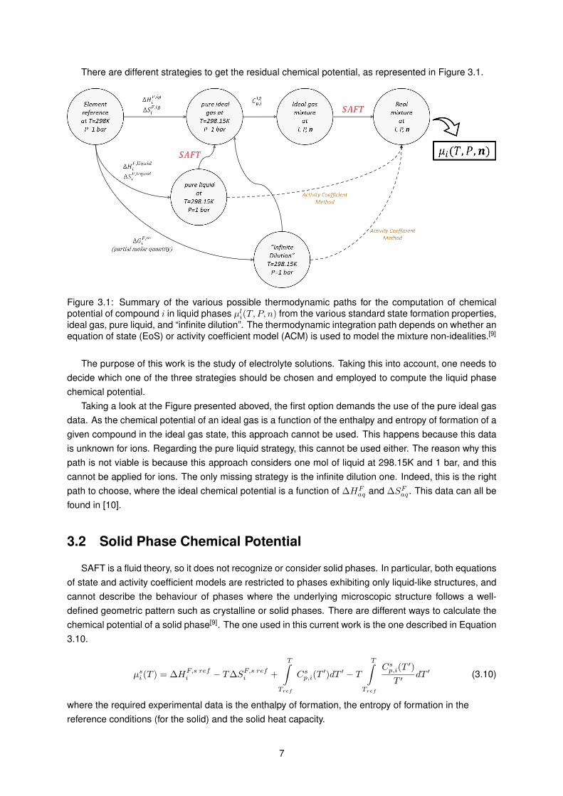
There are different strategies to get the residual chemical potential, as represented in Figure 3.1.

Figure 3.1: Summary of the various possible thermodynamic paths for the computation of chemicalpotential of compound i in liquid phases µli(T, P, n) from the various standard state formation properties,ideal gas, pure liquid, and “infinite dilution”. The thermodynamic integration path depends on whether anequation of state (EoS) or activity coefficient model (ACM) is used to model the mixture non-idealities.[9]

The purpose of this work is the study of electrolyte solutions. Taking this into account, one needs todecide which one of the three strategies should be chosen and employed to compute the liquid phasechemical potential.

Taking a look at the Figure presented aboved, the first option demands the use of the pure ideal gasdata. As the chemical potential of an ideal gas is a function of the enthalpy and entropy of formation of agiven compound in the ideal gas state, this approach cannot be used. This happens because this datais unknown for ions. Regarding the pure liquid strategy, this cannot be used either. The reason why thispath is not viable is because this approach considers one mol of liquid at 298.15K and 1 bar, and thiscannot be applied for ions. The only missing strategy is the infinite dilution one. Indeed, this is the rightpath to choose, where the ideal chemical potential is a function of ∆HF

aq and ∆SFaq. This data can all befound in [10].

3.2 Solid Phase Chemical Potential

SAFT is a fluid theory, so it does not recognize or consider solid phases. In particular, both equationsof state and activity coefficient models are restricted to phases exhibiting only liquid-like structures, andcannot describe the behaviour of phases where the underlying microscopic structure follows a well-defined geometric pattern such as crystalline or solid phases. There are different ways to calculate thechemical potential of a solid phase[9]. The one used in this current work is the one described in Equation3.10.

µsi (T ) = ∆HF,s refi − T∆SF,s refi +

T∫Tref

Csp,i(T′)dT ′ − T

T∫Tref

Csp,i(T′)

T ′dT ′ (3.10)

where the required experimental data is the enthalpy of formation, the entropy of formation in thereference conditions (for the solid) and the solid heat capacity.

7

8

Chapter 4

SAFT γ - Mie Equation of State

4.1 Evolution of Equations of State

Since the formulation of the ideal gas law and the Van der Waals conception for real gases, manyother equations of state have been developed in order to obtain rigorous predictions for phase equilibria,single phase properties and activity coefficients. Many followed the Van der Waals framework andthose developed thermodynamic models known as cubic equations of state. However, this type ofequations has some limitations and does not predict properly the properties of associating and non-spherical molecules. The main reason for this deficiency is that the cubic equations of state do nottake into account the shape of the molecules and assume that all the molecules can be representedas spheres, especially when dealing with large molecules. Moreover, they are a good approximationfor simple molecules that interact through London dispersion, but, with more complex molecules andinteractions the model breaks down. Apart from that, it is also known that they do not provide accurateresults when trying to obtain second derivative properties.

The main difference between the previous models and Statistical Associating Fluid Theory (SAFT)is that this last equation is underpinned by a physically realistic representation of the molecule thatincludes not only their shape but also their sizes and interactions between molecules (Including hydrogenbonding). The SAFT Equation of State (EoS) is a perturbation theory and has its roots in the First orderthermodynamic perturbation theory (TPT1) of Wertheim for associating and chain fluids. It provides aframework that allows the calculation of different properties of a system based on the knowledge of amonomeric reference fluid. This means that to obtain a given property, this EoS evaluates the propertyfor the reference fluid and then ”estimates” perturbations.

In SAFT, molecules are modelled as chains of bonded spherical segments interacting via an attrac-tive potential with short-range sites placed on the segments.[2]. Each group is then characterized bydifferent parameters as will be explained in the following topic.

There are different versions of SAFT and their main difference is in the choice of their intermolecularpotential for the sphere-sphere interactions. These interactions can be, for example, Lennard-Jones,Square-Well and Mie Potential. The SAFT γ - Mie framework was the approach used in this work, andso, its terms will be explained below.

4.2 Molecular model and intermolecular potential

The interactions between molecules need to be modelled as accurately as possible and differentcontributions based on the electrostatics, such as dispersion interactions and those arising from the

9

different multipole moments, need to be taken into account to describe the behaviour of molecules.[7]

As long as we have matter, we have two main types of forces: attractive and repulsive. Many potentialmodels have been developed, by combining different repulsive and attractive parts, with some commonfeatures: most repulsive terms tend to infinity at short separations, preventing a complete overlap of twomolecules, and the attractive terms tend to zero at infinity, so that the energy is not infinite.[7]

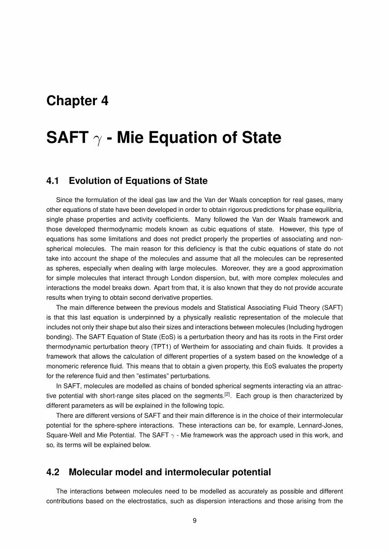
As was previously stated, SAFT γ - Mie is a variant of the general SAFT framework. This formulationis based on a generalised Lennard-Jones potential, or so called Mie-Potential, and takes into accounta group contribution approach. With this, molecules are described in terms of the functional groups,whereby the functional groups are assumed to behave independently of the molecule structure on whichthey are found.[9]

Overall, Group Contribution (GC) approaches consider that molecules are divided into different func-tional groups. This theory is underlined by the fact that all the molecular properties can be calculatedas a sum of the different contributions of the different functional groups, and that these group proper-ties remain the same even if they appear in a different host molecule. There are a set of parametersthat characterize these functional groups, namely the shape factor, Sk that describes the group non-sphericity, and some parameters related with the intermolecular potentials.

Figure 4.1: SAFT γ - Mie group contribution representation[11]

The Lennard-Jones potential describes the interaction of two neutral particles in terms of energy.These particles are subject to two opposing forces: attractive and repulsive. Although this model hassometimes been found too poor to describe the repulsive potential, it is widely used as a building blockof many force fields due to its computational expediency. The equation that describes this model is givenin 4.1

ΦLJkl (rkl) = Cklεkl

[ (σklr

)12

−(σklr

)6 ](4.1)

where σkl is the segment diameter (at which the potential is zero) and εkl is the depth of the potentialwell and it is a measure of the attraction that two particles have for each other. The term with the powerof 12 represents the repulsive forces, whereas the term with the power of 6 represents the attractiveforces.

A more versatile option is the Mie intermolecular potential, ΦMie, with adjustable attractive and repul-sive exponents. The advantage of the Mie potential lies in its soft-core variable range. The Mie potentialcan be described as:

ΦMiekl (rkl) = Cklεkl

[ (σklr

)λrkl−(σklr

)λakl ](4.2)

10

with:

C =λrkl

λrkl − λakl

(λrklλakl

) λaklλrkl−λa

kl

(4.3)

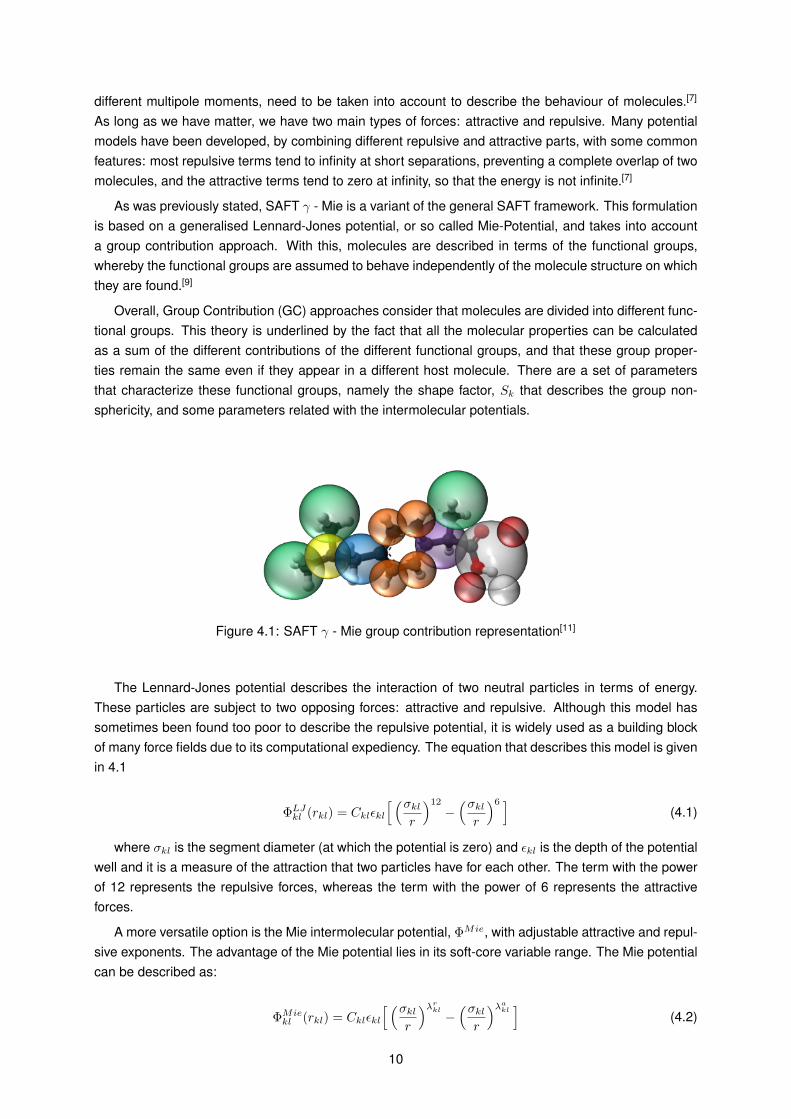
where λrkl and λakl are the repulsive and attractive exponents of the unlike interactions. The pre-factorCkl is a function of the exponents of the potential and ensures that the minimum interaction is given by−εkl. A graphical representation of the Mie Potential is given in figure 4.2:

Figure 4.2: Mie potential representation in function of the distance between two particles

In case of the existence of different groups in the same mixture we also need to consider the crossinteractions, like the cross εkl. In general, when dealing with mixtures with different groups, the exis-tent interactions are divided into two groups: self-interactions (for groups of the same type) and cross-interactions (for groups of different types).

4.3 SAFT γ - Mie: free energy contributions

The total Helmholtz free energy A of a mixture of heteronuclear associating molecules from differentMie segments can be written as a sum of different contributions. The original SAFT equation just takesinto account the first four terms of equation 4.4 . However, when dealing with electrolyte mixtures twomore terms need to be added, namely the ion term (that considers the ion-ion interactions) and the Bornterm (related to the process of charging the ionic species). As a result, a ”new” formulation of the SAFTEoS is presented below.

A

NkbT=Aideal

NkbT+Amono

NkbT+Achain

NkbT+Aassoc.

NkbT+ABorn

NkbT+

AIon

NkbT(4.4)

where Aideal stands for the free energy of an ideal gas, Amono. is the term accounting for interactionsbetween monomer segments, Achain is the contribution to the free energy for the formation of molecules,Aassoc. is the term accounting for the association interactions, ABorn is the Helmholtz free energy associ-ated with the process of charging the ions incorporated in the solvent, AIon is the Helmholtz free energyrelated with electrostatic interactions between charged species, N is the total number of molecules, kBis the Boltzmann constant and T is the absolute temperature.

As was stated above, the monomer fluid consists of spherical hard segments to which dispersionforces are added and chains can be formed through covalent bonds. A perturbation scheme is presentedin 4.3.

11

ADielectric = 0

ADisch.

ACharge

ADisp

AIon

AAssocAChain

AIdeal

9)

4)

3)

7)

6)

1)

8)

5)

2)

AHS

Born cycle

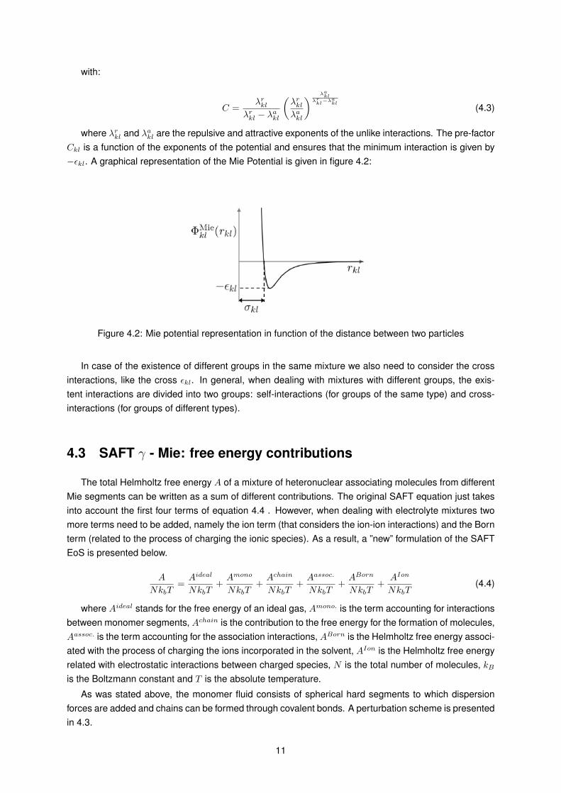
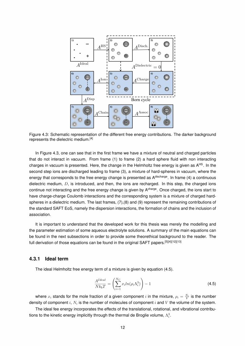
Figure 4.3: Schematic representation of the different free energy contributions. The darker backgroundrepresents the dielectric medium.[4]

In Figure 4.3, one can see that in the first frame we have a mixture of neutral and charged particlesthat do not interact in vacuum. From frame (1) to frame (2) a hard sphere fluid with non interactingcharges in vacuum is presented. Here, the change in the Helmholtz free energy is given as AHS. In thesecond step ions are discharged leading to frame (3), a mixture of hard-spheres in vacuum, where theenergy that corresponds to the free energy change is presented as Adischarge. In frame (4) a continuousdielectric medium, D, is introduced, and then, the ions are recharged. In this step, the charged ionscontinue not interacting and the free energy change is given by Acharge. Once charged, the ions start tohave charge-charge Coulomb interactions and the corresponding system is a mixture of charged hard-spheres in a dielectric medium. The last frames, (7),(8) and (9) represent the remaining contributions ofthe standard SAFT EoS, namely the dispersion interactions, the formation of chains and the inclusion ofassociation.

It is important to understand that the developed work for this thesis was merely the modelling andthe parameter estimation of some aqueous electrolyte solutions. A summary of the main equations canbe found in the next subsections in order to provide some theorethical background to the reader. Thefull derivation of those equations can be found in the original SAFT papers.[5][4][12][13]

4.3.1 Ideal term

The ideal Helmholtz free energy term of a mixture is given by equation (4.5).

AIdeal

NkbT=

(NC∑i=1

xiln(ρiΛ3i )

)− 1 (4.5)

where xi stands for the mole fraction of a given component i in the mixture, ρi = NiV is the number

density of component i, Ni is the number of molecules of component i and V the volume of the system.

The ideal fee energy incorporates the effects of the translational, rotational, and vibrational contribu-tions to the kinetic energy implicitly through the thermal de Broglie volume, Λ3

i .

12

4.3.2 Monomer term

The monomer term accounts for the interactions between each segment, or monomer (whether it isan atom, a molecule or a GC) and for that reason requires that an intermolecular potential is defined. Inthe SAFT γ - Mie framework, the monomer contribution of the Helmholtz free energy is obtained as athird-order perturbation expansion. [12]

AMono

NkbT=

AHS

NkbT+

A1

NkbT+

A2

NkbT+

A3

NkbT(4.6)

where AHS stands for the hard sphere Helmholtz free energy of the mixture and is given by:

AHS

NkBt=

(NC∑i=1

xi

NG∑k=1

νk,iν∗kSk

)aHS (4.7)

where NC is the number of components, NG is the number of group types, νk,i is the number ofoccurrences of group k, ν∗k is the number of identical segments that form group k and aHS is the dimen-sionless contribution to the hard-sphere free energy per segment. This last parameter can be obtainedusing the expression of Boublık and Mansoori. [12]

A1,A2 and A3 correspond to the attractive perturbation terms. The first order term A1 of the per-turbation expansion correlates to the mean attractive energy per molecule and, as for the hard-sphereterm, it is obtained as a summation of the contributions to the mean-attractive energy per segment a1:

A1

NkBT=

1

kBT

(NC∑i=1

xi

NG∑k=1

νk,iν∗kSk

)a1 (4.8)

where

a1 =

NG∑k=1

NG∑l=1

xs,kxs,la1,kl (4.9)

with xs,k standing for the fraction of segments of a group of type k in the mixture, and a1,kl for pairwiseinteractions between groups k and l over all types of functional groups present in the system.

The second order perturbation is calculated using the improved Macroscopic compressibility approx-imation (MCA) with the modification proposed by Paricaud. [5] This particular term accounts for the localfluctuation in the attractive interactions and is obtained as:

A2

NkBT=

(1

kBT

)2(NC∑i=1

xi

NG∑l=1

xs,kxs,la2,kl

)(4.10)

with,

a2 =

NG∑k=1

NG∑l=1

xs,kxs,la2,kl (4.11)

Last but not least, an empirical expression is used for the third order perturbation term, A3, withcoefficients obtained to reproduce the critical point and fluid-phase equilibrium of Mie fluids.[5] This termis obtained for the contribution per segment a3 as[12]:

A3

NkBT=

(1

kBT

)3(NC∑i=1

xi

NG∑l=1

νk,iν∗kSk

)a3 (4.12)

13

and,

a3 =

NG∑k=1

NG∑l=1

xs,kxs,la3,kl (4.13)

4.3.3 Chain term

The SAFT approach accounts for chain length by taking the limit of complete bonding in Wertheim’sTPT1. By including the chain term, the SAFT EoS considers the free energy contributions due to theformation of chains made of monomer segments. In the case of a mixture, the expression is given as [5]:

Achain

NkBT= −

Nc∑i=1

xi(mseg,i − 1)lngMieii (σi) (4.14)

where mseg,i stands for the number of segments per chain and lngMieii takes into account the Radial

Distribution Function (RDF) of the monomeric Mie fluid system at contact σi.

4.3.4 Association term

Associating fluids are able to form clusters of associated molecules. Therefore, the SAFT model forassociating fluids not only accounts for monomers but also for associated clusters.

The association contribution has its roots in the Weirtheim’s first order thermodynamic perturbationtheory (TPT1) and it is motivated because some molecules tend to ”stick together”. As a consequence,the AAssociation term accounts for the free energy due to the association between molecules through thebonding sites and can be calculated by:

AAssociation

NkBT=

NC∑i=1

xi

NG∑k=1

νk,i

NST,k∑a=1

nk,a

(lnXi,k,a +

1−Xi,k,a

2

)(4.15)

This fraction is obtained through a set of equations called mass-action equations, which essentiallyresult from a mass balance to association sites.

4.3.5 Born Contribution

The change in the free energy of a system, due to the insertion of all ions in the dielectric medium,is given by the free energy of solvation.[5] In other words, one can say that the Born solvation energycan be defined as the change in the free energy that results from the electrostatic interactions whenions are transferred from vacuum into a dielectric medium at infinite dilution.[4] Though simplistic, thetheory used to describe the process of solvation is the Born approach. Despite its simplicity, this methodcaptures the basic thermodynamic features and gives good estimates. Overall, in his original derivationa thermodynamic cycle is proposed in which the work of discharging the particle in vacuum and thework of recharging it in the medium are incorporated, while neglecting the work required to transfer theuncharged particle into the solvent.[4] The final result, at infinite dilution, leads to:

µBorni = − e2

4πε0

(1− 1

D

)(z2i

σBorni

)(4.16)

where µBorni is the chemical potential of a certain ion, i, in solution, e is the elementary charge(1.602× 10−19C), ε0 is the vacuum permittivity (8.854× 10−12C2Jm−1), D is the relative permittivity of a

14

uniform dielectric medium, zi is the bearing charge, and σBorni is the diameter of a non-polarized spherethat represents the ion.

In equations based on primitive model expressions, the accuracy of the Couloumbic free energycontributions (AIon and ABorn) is crucially dependent on the usage of accurate values for the dielectricconstant that is used in place of an explicit accounting of the solvent electric properties. There are anumber of rigorous models to obtain the dielectric constant, however they are not easy to implement,and generally, they require new added adjustable parameters. Instead, the relative static permittivityD iscalculated with a Harvey-Prausnitz model. This correlative model depends on the solvent composition,density, and temperature, and thereby exhibits an implicit dependence on the ion concentration. Thismodel suggests that there is a relationship between the dielectric constant and the density of many polarmedia.[4],[5]

D = 1 + ρsolvd (4.17)

where d is a solvent-dependent parameter (calculated through the following equation) and ρsolv isthe density of the solvent.

d = dV

(dTT− 1

)(4.18)

where dV is a volume parameter and dT a temperature parameter. Both of them are componentspecific parameters.

Considering a constant volume and temperature, and assuming the same change in free energy forthe insertion of each of the ions, the Helmholtz free energy change is given by:

ABorn = − e2

4πε0

(1− 1

D

) ∑ion,i=1

Niz2i

σBorni

(4.19)

4.3.6 MSA Contribution

The ionic contribution to the Helmholtz free energy illustrates the replacement of the solvent by adielectric medium in which Coulombic interactions are screened.[4] This means that ion-ion interactionsare expressed with a Coulomb potential in a dielectric medium, i.e.

uion(rij) =e2

4πε0D

ZiZjrij

(4.20)

where rij represents the centre centre distance between charges i and j. There is more than onetheory when considering electrolyte modelling: the primitive one and the non-primitive one. In the case ofthe primitive model either the Debye-Huckel theory or the Mean Spherical Approximation (MSA) is usedand leads to accurate and similar results. Applying the MSA approach, the change in the Helmholtzfree energy due to electrostatic interactions between charged species within the MSA formalism can beexpressed as:

Aion = UMSA +Γ3kBTV

3π(4.21)

where UMSA stands for the MSA contribution to the internal energy U , and Γ is the screening lengthof the electrostatic forces. The MSA internal energy can be obtained by:

UMSA = − e2V

4πε0D

[Γ

V

nion∑i=1

(NiZ

2i

1 + Γσi

)+

π

2∆ΩP 2

n

](4.22)

15

with ∆ representing the packing fraction of the ions as a function of their diameter, σ3i :

∆ = 1− π

6V

nion∑i=1

Niσ3i (4.23)

With regard to the Pn and Ω functions, they are coupling parameters, where Pn couples to the chargeof the ions, whereas Ω relates to the packing fraction of the ions.[5] They can both be obtained by thefollowing equations:

Pn =1

ΩV

nion∑i=1

NiσiZi1 + Γσi

(4.24)

Ω = 1 +π

2∆V

nion∑i=1

Niσ3i

1 + Γσi(4.25)

Ultimately, the screening length, given by Γ, is a function of the relative static permittivity and theeffective charge Qi(Γ) of the ions:

Γ2 =πe2

(4πε0)DkBTV

nion∑i=1

NiQ2i (4.26)

where the effective charge is related to the electric charge of the individual species and the Pn

coupling parameter:

Qi =Zi − σ2

i Pn( π2∆ )

1 + Γσi(4.27)

To establish Γ it is necessary to run an iterative procedure, in which the initial guess is given byΓ0. This initial guess is, on the other hand, obtained by the Debye-Huckel formulation, as seen in thefollowing equation:

Γ0 =κ

2= 0.5

√√√√ e2

4Dε0V kBT

nion∑i=1

NiZ2i (4.28)

where κ is the inverse Debye-Huckel length.

16

Chapter 5

Development of model parametersand analyses of the systems ofinterest

5.1 Description of parameters

The SAFT γ- Mie framework is used to describe the behaviour of electrolyte solutions. Variouselectrolyte solutions are considered focusing on a broad set of experimental data. The goal of this workis to determine the best combination of thermodynamic properties to include in the parameter regressionprocedure to ensure that the resulting model parameters can capture all the desired results.

The EoS is formulated such that model parameters are ion based (as opposed to salt based), whichallows for the properties of multiple salts to be calculated with fewer parameters.[8]

In this work ions are modelled as spheres consisting of a single segment (mseg,i = 1) of diameterσi and carrying a single point charge (qi = Zie). All the ions experience dispersion interactions, rep-resented by Mie potentials, both with the other ions in solution and with the neutral species. Water isrepresented as a spherical molecule with four off-centre association sites.[5]

Figure 5.1: Schematic representation of the model used for the like and unlike interactions between ion-ion and ion-water. (NaCl example) The associative sites are labelled as e and H, typically representingeither a lone-pair of electrons on an electronegative atom or hydrogen atoms in the functional group.

The adjustable parameters for the like-interactions include the diameter σi and the interaction energyεii, whereas the adjustable unlike interactions include the interaction energy between two different ions,

17

εij and between an ion with the solvent, εi−water. With regard to the repulsive and attractive exponentsthey were set with the value of 12 and 6, respectively, as described in the Lennard-Jones potential. Thisapproach allows the reduction of the number of parameters to be estimated and, as will be seen, leadsto good results.

In order to compensate for some of the shortcomings of the Born term, and hence capture the solva-tion effects more accurately, an extra adjustable parameter for ions called the ionic diameter increment∆σi was found to be necessary in some previous works[8], which is related to the ion group diameterthrough:

σBorni = σi + ∆σi (5.1)

Finally we have found that it is necessary to consider that cross interactions can be temperaturedependent. As a consequence, another adjustable parameter was considered: epsilon expansion coef-ficient, B. If we take the εi−water as an example, we can see in equation 5.2 how it can be calculated.

εi−waterk

=ε0,i−water

k+Bi−waterkT

(5.2)

where ε0,i−water accounts for the ion-water interaction parameter.

5.2 Experimental Data

Experimental data is not only necessary to the estimation of parameters for a thermodynamic modelbut also to validate the model. Before starting the parameter estimation several data had to be gatheredand diverse literature was used. For this work experimental data on solubilities, liquid phase densities,mean activity coefficients, osmotic coefficients, heat capacities of the solid and liquid phases and heatsof dilution was needed.

One important thing to understand is that some of these data, like the solid properties, had to beprovided to the model. This was found to be necessary because SAFT is a fluid theory, and so, thetheory cannot calculate these data by itself.

For the construction of the databank, it was necessary to have:

• Ions enthalpy and entropy of formation [10]

• Molecular weights of ions and salts [14]

• Solid enthalpy and entropy of formation [10]

• Solid heat capacities [14],[15]

On the other hand, it was also necessary to obtain some data to build the model and to fit the diverseparameters. Among that data we have:

• Salts solubilities in water [16],[17],[18],[19],[20]

• Solution liquid phase densities [21]

• Liquid phase heat capacities [22]

• Enthalpies of dilution [22]

Last but not least, there were properties that were not used in the modelling but were verified in orderto see if the predicted results were in line with the expected.

18

• Mean Activity Coefficients [23]

• Osmotic Coefficients [23]

5.3 Systems of interest

One of the decisions that had to be made was which salts would be studied and considered to buildthe desired model. In the previous section, all the necessary experimental data was introduced to buildthe databank and to proceed with the parameter estimation. In order to find out in which salts the studywould be based on, diverse literature was consulted in order to choose which salts could be considered.

In Table 5.1, all the results of the literature review are summed up. From all the ions combinations,the only resulting salts that could be considered in this study were the ones covered with a blue shading.For the ones covered with a red shading, either it was not possible to find the necessary data, likesolubilities, formation enthalpies and entropies and solid phase heat capacities, or the available datawas not consistent and reliable. Regarding the yellow shaded cells, the presented salts are alwaysfound in the hydrate form. Solid heat capacities and formation properties were not found for thesecompounds, and for that reason they could not be considered and studied. In order to overcome thisproblem, it was attempted to fit solid heat capacities for hydrates, however, the obtained results were nottrustworthy. (See Appendix B)

Table 5.1: Literature review results. The blue shaded cells have to do with the salts that can be consid-ered to build the model, the yellow shaded cells represent the salts that are only in the hydrate form in thestudied conditions, and the red shaded cells represent the salts for which it wasn’t found the necessarydata.

F− Cl− Br− I− NO−3 ClO−4 SO2−4

Li+ LiF LiCl LiBr LiI LiNO3 LiClO4 Li2SO4

Na+ NaF NaCl NaBr NaI NaNO3 NaClO4 Na2SO4

K+ KF KCl KBr KI KNO3 KClO4 K2SO4

Rb+ RbF RbCl RbBr RbI RbNO3 RbClO4 Rb2SO4

Cs+ CsF CsCl CsBr CsI CsNO3 CsClO4 Cs2SO4

Mg2+ MgF2 MgCl2 MgBr2 MgI2 Mg(NO3)2 Mg(ClO4)2 MgSO4

Ca2+ CaF2 CaCl2 CaBr2 CaI2 Ca(NO3)2 Mg(ClO4)2 CaSO4

Sr2+ SrF2 SrCl2 SrBr2 SrI2 Sr(NO3)2 Sr(ClO4)2 SrSO4

Ba2+ BaF2 BaCl2 BaBr2 BaI2 Ba(NO3)2 Ba(ClO4)2 BaSO4

Mn2+ MnF2 MnCl2 MnBr2 MnI2 Mn(NO3)2 Mn(ClO4)2 MnSO4

NH+4 NH4F NH4Cl NH4Br NH4I NH4NO3 NH4ClO4 (NH4)2SO4

Cd2+ CdF2 CdCl2 CdBr2 CdI2 Cd(NO3)2 Cd(ClO4)2 CdSO4

As a first approach, the ions that were parametrized were Na+, K+, Cl− and Br− and, for thatreason, the data needed is referred to NaCl, KCl, NaBr and KBr.

Still regarding the solubility data, it is important to underline that the range of temperatures used wasbetween 25 and a 100 Celsius degrees.

The estimation of the group parameters is carried out using the gSAFT Material Modeller (gSAFTmm)by minimizing an objective function. The objective function applied is given by:

19

fobj =

NP∑i=1

(scali − s

expi

scali

)2

+

NP∑i=1

(ρcali − ρ

expi

ρcali

)2

+

NP∑i=1

(Cpcali − Cp

expi

Cpcali

)2

(5.3)

+

NP∑i=1

(∆Hcal

d,i −∆Hexpd,i

∆Hcald,i

)2

where si stands for the solubility of a given salt, ρi for the density, Cpi for the heat capacity and ∆Hd,i

for the dilution enthalpy.

One interesting thing to say is that, when computing the different adjustable parameters, it is possibleto give different weights to the different properties that are being used. This means that properties withlower weights will have a lower impact in the results of the final model.

20

Chapter 6

Parameter Estimation Strategy andResults

To introduce this chapter it is important to say that not all of the obtained results and plots are shownin each step of the parameter estimation strategy. Those information is only available in the mentionedAppendixes. The reason why it was chosen to present the results in this way is due to the fact that, aswill be seen, we can only obtain all the desired results by combining data on every property (solubilities,liquid phase densities, liquid phase heat capacities and dilution enthalpies).

6.1 Estimation using solubility

During all the parameter estimation startegy it was considered that the solubility of inorganic com-pounds in water was crucial to be described.

In order to obtain these results, the parameters for all the ions were fitted at the same time and onlythe data on salts solubilities was used. The model proved to be able to accurately fit the results withoutit being necessary to include all the available experimental points.

Regarding the considered fitted parameters, in this particular case it was only needed to estimatethe values of:

• σi• εii• εij• εi−water

All the regressed parameters can be seen in Appendix C.1, Tables C.1 and C.2 .The obtained results are presented in Figure 6.1 and, as can be seen, SAFT γ-Mie could fit the

results properly. One interesting result is the NaBr solubility as a function of temperature. NaBr

for temperatures below 60°C is in a hydrate form (NaBr.2H2O).[19],[16] As was already stated, hydrateforms are difficult to study due to the lack of information on the solid form heat capacities as a functionof temperature. However, taking into account only the hydrate data at 25°C the problem is overcome(check Equation 3.10), and as can be seen, the model is able to predict the right solubility behaviour forthe other temperatures as well.

21

300 320 340 360

26.5

27

27.5

28

Temperature (K)

Sol

ubili

ty(g

solute/100g s

olution) NaCl Solubility

(a)

300 320 340 36048

50

52

54

56

Temperature (K)

Sol

ubili

ty(g

solute/100g s

olution) NaBr Solubility

(b)

300 320 340 360

25

30

35

Temperature (K)

Sol

ubili

ty(g

solute/100g s

olution) KCl Solubility

(c)

300 320 340 360

40

45

50

Temperature (K)

Sol

ubili

ty(g

solute/100g

solution) KBr Solubility

(d)

Figure 6.1: Solubility of a salt depending on the temperature, taking into account only experimental dataon solubility. The different plots have both experimental () and SAFT predictions data (−).

Looking beyond these results, it was of interest to know if only by fitting the parameters to the solubilityvalues, it would be possible to predict all the other properties. The obtained results were evaluated formean activity coefficients, liquid phase densities, liquid phase heat capacities, osmotic pressures andenthalpies of dilution. Unfortunately none of these properties revealed good results when compared withall the experimental data. All the results can be analysed in the Appendix C.1.

6.2 Estimation using solubility and liquid phase density

The second startegy was to adjust the the liquid phase density. The amount of a species in a givenvolume depends on its size, and because of that, sigma values and densities are related with oneanother. In fact, when comparing the results of the previous approach with the final ones it is possible tosee that the final sigma values (accounted by the Born sigma) are very different.

Approach 6.2.1

It was of interest to understand if it would be possible to fit the results to solubility and density whenusing a reduced set of adjustable parameters. Therefore, it was studied if it would be possible to reachaccurate results when regressing the same parameters as before: σi, εii, εij and εi−water. The results(presented in the Appendix C.2) proved that the objective function was not sufficiently low to reproduce

22

the experimental results in such a good way as before. The desire to improve these results resulted in asecond attempt of parameters fitting.

In view of the above, in Figure 6.2 it is possible to analyse the change in the solubility results for theNaCl.

300 320 340 360

26.5

27

27.5

28

Temperature (K)

Sol

ubili

ty(g

solute/100g s

olution) Solubility

(a)

300 320 340 360

26.5

27

27.5

28

Temperature (K)

Sol

ubili

ty(g

solute/100g s

olution) Solubility + Density

(b)

Figure 6.2: Comparison of solubilities predictions for NaCl. (a) Model-Fitting to Solubility, (b) Model-Fitting to Solubility and Liquid Phase Density (Approach 1)

The quantitative results can be observed in the following table.

Table 6.1: Comparison of solubility results for NaCl and corresponding %∆.

Solubility Solubility + Density

Temperature (K)Experimental Solubilities

gsolute/100gsolutionSAFT %∆ SAFT %∆

298.15 26.45 26.44 0.03 26.25 0.76303.15 26.52 26.50 0.06 26.36 0.60313.15 26.67 26.66 0.03 26.60 0.27323.15 26.84 26.85 0.05 26.84 0.01333.15 27.03 27.07 0.15 27.09 0.24343.15 27.25 27.30 0.19 27.35 0.35353.15 27.50 27.54 0.14 27.59 0.34363.15 27.78 27.78 0.01 27.83 0.19373.15 28.05 28.01 0.14 28.06 0.05

Approach 6.2.2

In order to keep good results for solubility, a new parameter was considered adjustable: ∆σi. Byadding this parameter, as was expected, the solubility values could be once again obtained with ac-curacy. This happens because the same propreties were being considered but a new parameter wasadded.

All the regressed parameters can be seen in the Appendix C.2, Tables C.3 and C.4 .

23

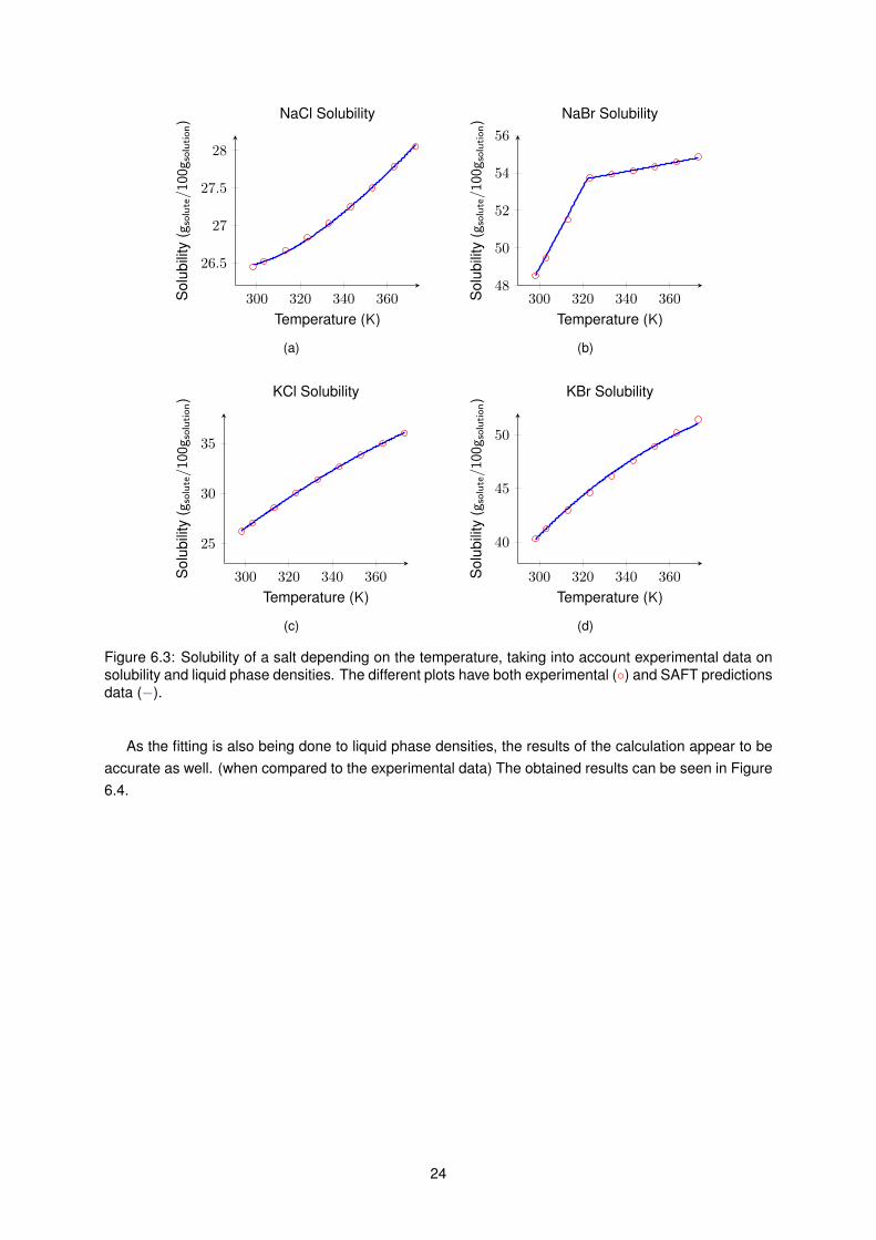
300 320 340 360

26.5

27

27.5

28

Temperature (K)

Sol

ubili

ty(g

solute/100g s

olution) NaCl Solubility

(a)

300 320 340 36048

50

52

54

56

Temperature (K)

Sol

ubili

ty(g

solute/100g s

olution) NaBr Solubility

(b)

300 320 340 360

25

30

35

Temperature (K)

Sol

ubili

ty(g

solute/100g s

olution) KCl Solubility

(c)

300 320 340 360

40

45

50

Temperature (K)

Sol

ubili

ty(g

solute/100g

solution) KBr Solubility

(d)

Figure 6.3: Solubility of a salt depending on the temperature, taking into account experimental data onsolubility and liquid phase densities. The different plots have both experimental () and SAFT predictionsdata (−).

As the fitting is also being done to liquid phase densities, the results of the calculation appear to beaccurate as well. (when compared to the experimental data) The obtained results can be seen in Figure6.4.

24

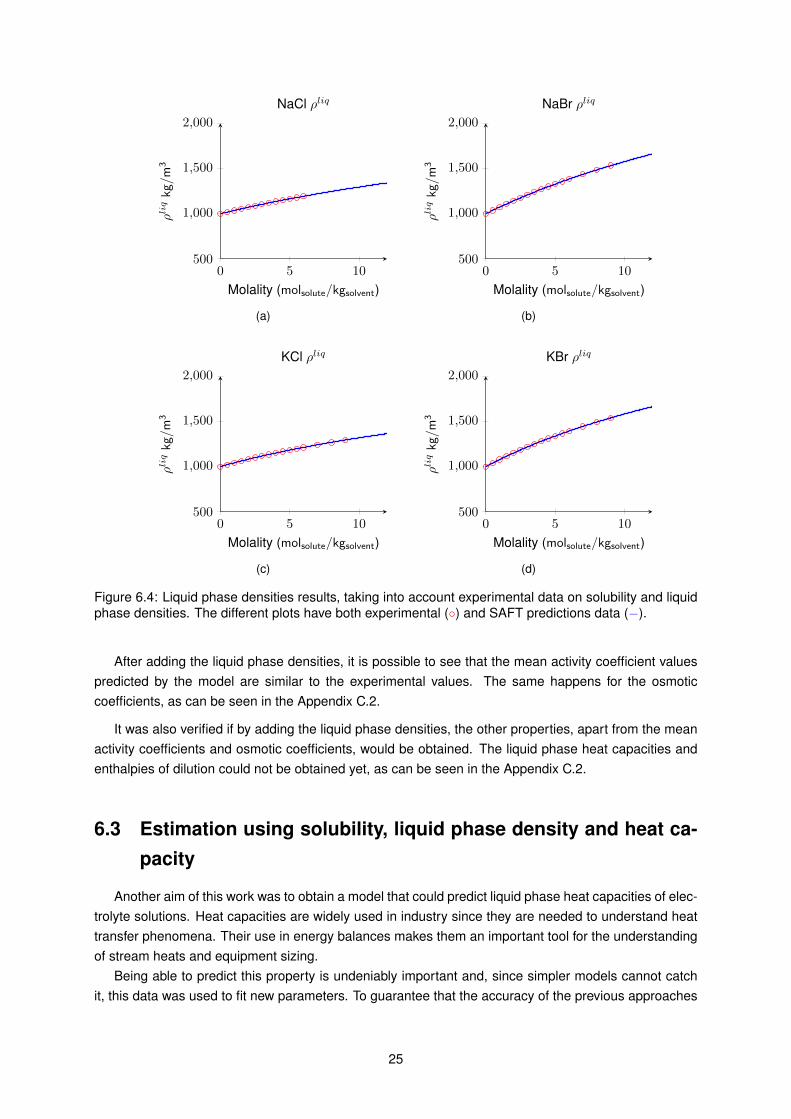
0 5 10500

1,000

1,500

2,000

Molality (molsolute/kgsolvent)

ρliqkg/m

3

NaCl ρliq

(a)

0 5 10500

1,000

1,500

2,000

Molality (molsolute/kgsolvent)

ρliqkg/m

3

NaBr ρliq

(b)

0 5 10500

1,000

1,500

2,000

Molality (molsolute/kgsolvent)

ρliqkg/m

3

KCl ρliq

(c)

0 5 10500

1,000

1,500

2,000

Molality (molsolute/kgsolvent)

ρliqkg/m

3

KBr ρliq

(d)

Figure 6.4: Liquid phase densities results, taking into account experimental data on solubility and liquidphase densities. The different plots have both experimental () and SAFT predictions data (−).

After adding the liquid phase densities, it is possible to see that the mean activity coefficient valuespredicted by the model are similar to the experimental values. The same happens for the osmoticcoefficients, as can be seen in the Appendix C.2.

It was also verified if by adding the liquid phase densities, the other properties, apart from the meanactivity coefficients and osmotic coefficients, would be obtained. The liquid phase heat capacities andenthalpies of dilution could not be obtained yet, as can be seen in the Appendix C.2.

6.3 Estimation using solubility, liquid phase density and heat ca-pacity

Another aim of this work was to obtain a model that could predict liquid phase heat capacities of elec-trolyte solutions. Heat capacities are widely used in industry since they are needed to understand heattransfer phenomena. Their use in energy balances makes them an important tool for the understandingof stream heats and equipment sizing.

Being able to predict this property is undeniably important and, since simpler models cannot catchit, this data was used to fit new parameters. To guarantee that the accuracy of the previous approaches

25

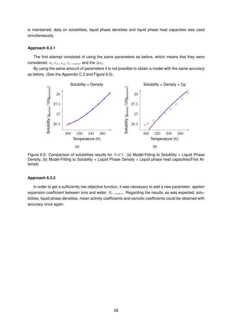
is maintained, data on solubilities, liquid phase densities and liquid phase heat capacities was usedsimultaneously.

Approach 6.3.1

The first attempt consisted of using the same parameters as before, which means that they wereconsidered: σi, εii, εij , εi−water and the ∆σi.

By using the same amount of parameters it is not possible to obtain a model with the same accuracyas before. (See the Appendix C.3 and Figure 6.5).

300 320 340 360

26.5

27

27.5

28

Temperature (K)

Sol

ubili

ty(g

solute/100g s

olution) Solubility + Density

(a)

300 320 340 360

26.5

27

27.5

28

Temperature (K)

Sol

ubili

ty(g

solute/100g s

olution) Solubility + Density + Cp

(b)

Figure 6.5: Comparison of solubilities results for NaCl. (a) Model-Fitting to Solubility + Liquid PhaseDensity, (b) Model-Fitting to Solubility + Liquid Phase Density + Liquid phase heat capacities(First At-tempt)

Approach 6.3.2

In order to get a sufficiently low objective function, it was necessary to add a new parameter: epsilonexpansion coefficient between ions and water, Bi−water. Regarding the results, as was expected, solu-bilities, liquid phase densities, mean activity coefficients and osmotic coefficients could be obtained withaccuracy once again.

26

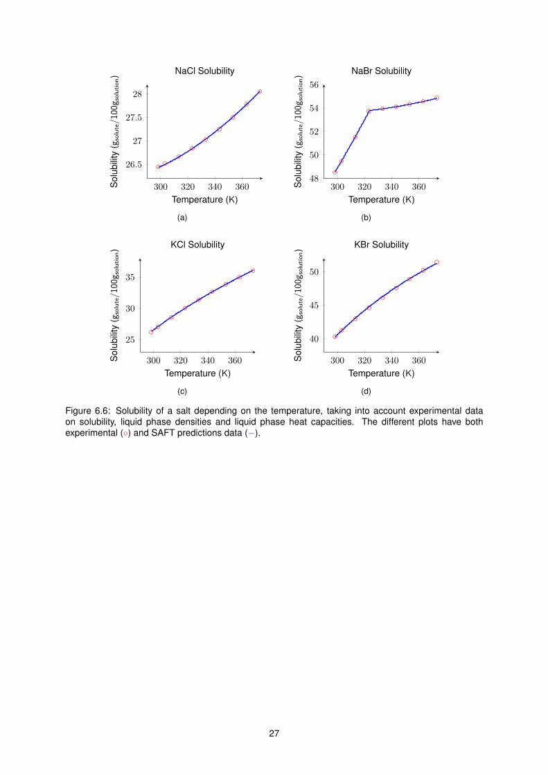
300 320 340 360

26.5

27

27.5

28

Temperature (K)

Sol

ubili

ty(g

solute/100g s

olution) NaCl Solubility

(a)

300 320 340 36048

50

52

54

56

Temperature (K)

Sol

ubili

ty(g

solute/100g s

olution) NaBr Solubility

(b)

300 320 340 360

25

30

35

Temperature (K)

Sol

ubili

ty(g

solute/100g s

olution) KCl Solubility

(c)

300 320 340 360

40

45

50

Temperature (K)

Sol

ubili

ty(g

solute/100g

solution) KBr Solubility

(d)

Figure 6.6: Solubility of a salt depending on the temperature, taking into account experimental dataon solubility, liquid phase densities and liquid phase heat capacities. The different plots have bothexperimental () and SAFT predictions data (−).

27

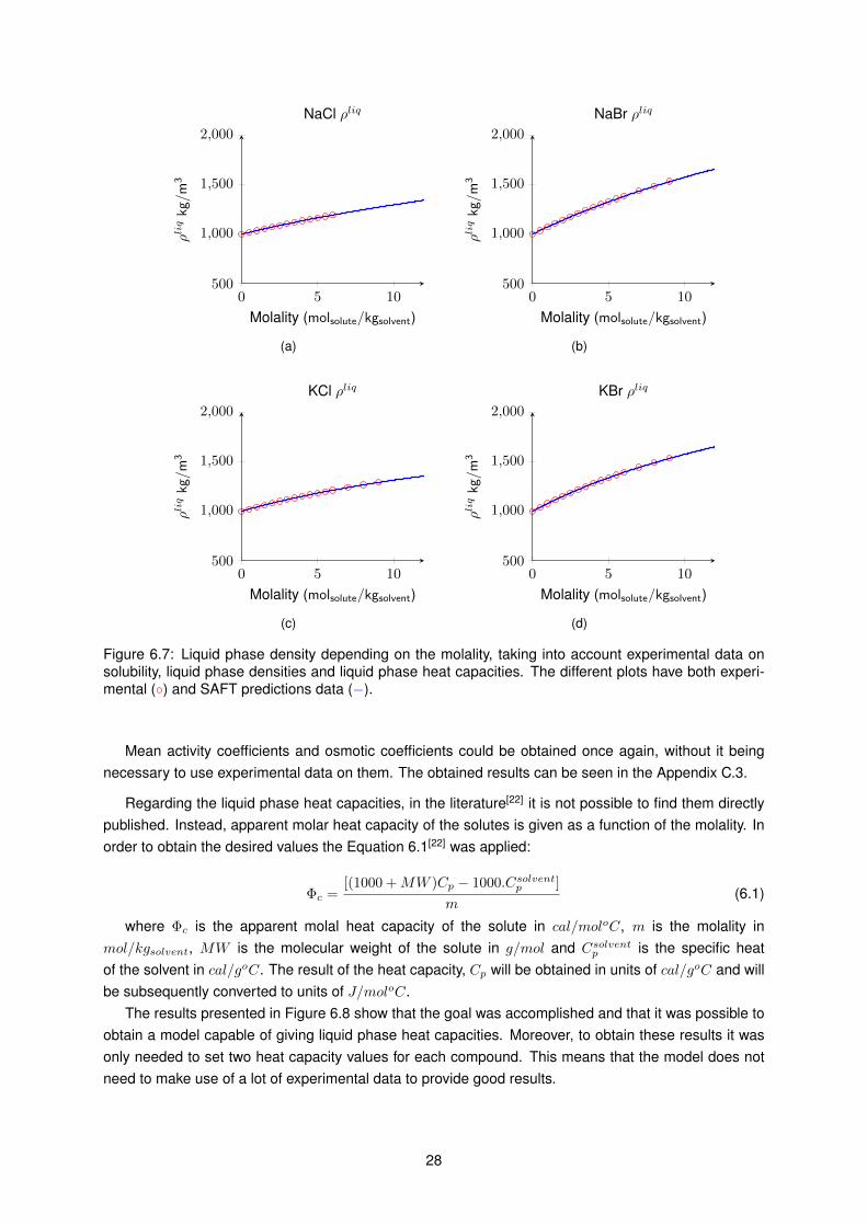
0 5 10500

1,000

1,500

2,000

Molality (molsolute/kgsolvent)

ρliqkg/m

3

NaCl ρliq

(a)

0 5 10500

1,000

1,500

2,000

Molality (molsolute/kgsolvent)

ρliqkg/m

3

NaBr ρliq

(b)

0 5 10500

1,000

1,500

2,000

Molality (molsolute/kgsolvent)

ρliqkg/m

3

KCl ρliq

(c)

0 5 10500

1,000

1,500

2,000

Molality (molsolute/kgsolvent)

ρliqkg/m

3

KBr ρliq

(d)

Figure 6.7: Liquid phase density depending on the molality, taking into account experimental data onsolubility, liquid phase densities and liquid phase heat capacities. The different plots have both experi-mental () and SAFT predictions data (−).

Mean activity coefficients and osmotic coefficients could be obtained once again, without it beingnecessary to use experimental data on them. The obtained results can be seen in the Appendix C.3.

Regarding the liquid phase heat capacities, in the literature[22] it is not possible to find them directlypublished. Instead, apparent molar heat capacity of the solutes is given as a function of the molality. Inorder to obtain the desired values the Equation 6.1[22] was applied:

Φc =[(1000 +MW )Cp − 1000.Csolventp ]

m(6.1)

where Φc is the apparent molal heat capacity of the solute in cal/moloC, m is the molality inmol/kgsolvent, MW is the molecular weight of the solute in g/mol and Csolventp is the specific heatof the solvent in cal/goC. The result of the heat capacity, Cp will be obtained in units of cal/goC and willbe subsequently converted to units of J/moloC.

The results presented in Figure 6.8 show that the goal was accomplished and that it was possible toobtain a model capable of giving liquid phase heat capacities. Moreover, to obtain these results it wasonly needed to set two heat capacity values for each compound. This means that the model does notneed to make use of a lot of experimental data to provide good results.

28

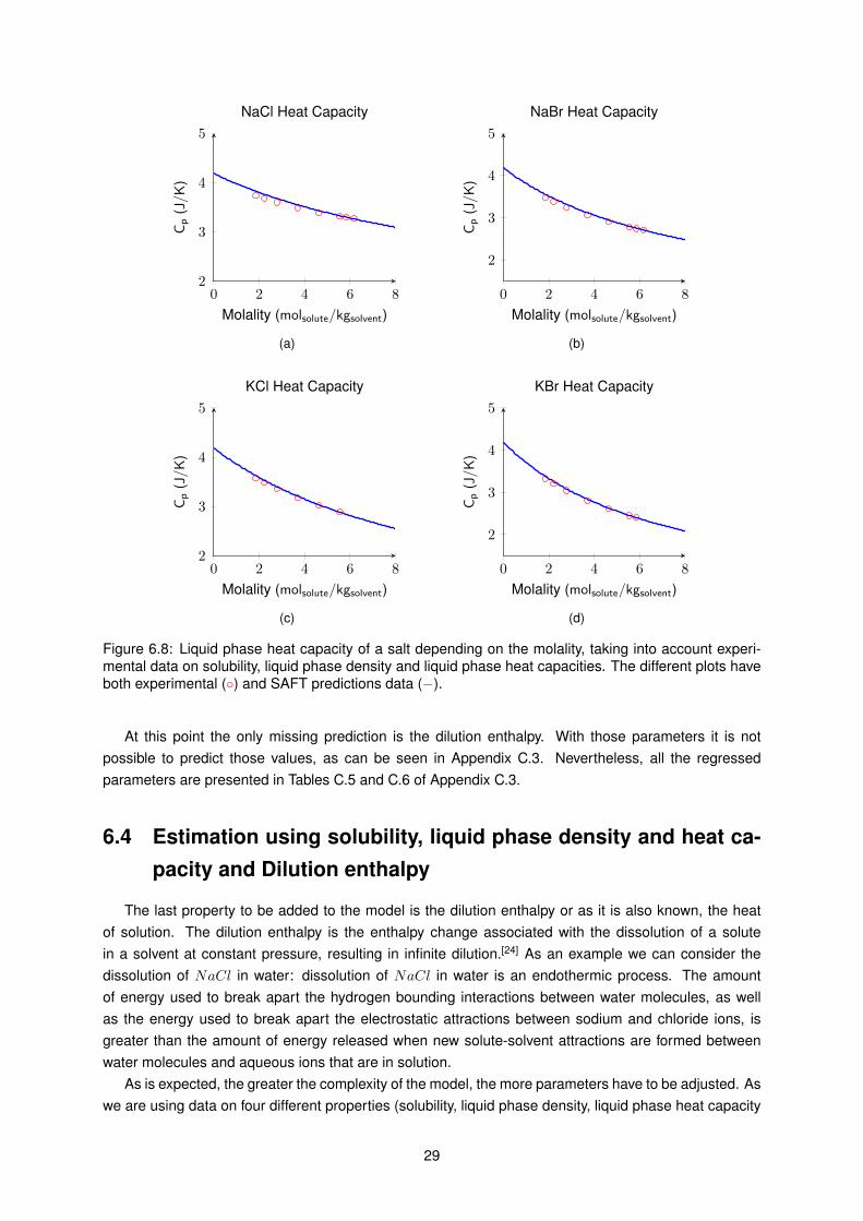
0 2 4 6 82

3

4

5

Molality (molsolute/kgsolvent)

Cp

(J/K

)

NaCl Heat Capacity

(a)

0 2 4 6 8

2

3

4

5

Molality (molsolute/kgsolvent)

Cp

(J/K

)

NaBr Heat Capacity

(b)

0 2 4 6 82

3

4

5

Molality (molsolute/kgsolvent)

Cp

(J/K

)

KCl Heat Capacity

(c)

0 2 4 6 8

2

3

4

5

Molality (molsolute/kgsolvent)

Cp

(J/K

)

KBr Heat Capacity

(d)

Figure 6.8: Liquid phase heat capacity of a salt depending on the molality, taking into account experi-mental data on solubility, liquid phase density and liquid phase heat capacities. The different plots haveboth experimental () and SAFT predictions data (−).

At this point the only missing prediction is the dilution enthalpy. With those parameters it is notpossible to predict those values, as can be seen in Appendix C.3. Nevertheless, all the regressedparameters are presented in Tables C.5 and C.6 of Appendix C.3.

6.4 Estimation using solubility, liquid phase density and heat ca-pacity and Dilution enthalpy

The last property to be added to the model is the dilution enthalpy or as it is also known, the heatof solution. The dilution enthalpy is the enthalpy change associated with the dissolution of a solutein a solvent at constant pressure, resulting in infinite dilution.[24] As an example we can consider thedissolution of NaCl in water: dissolution of NaCl in water is an endothermic process. The amountof energy used to break apart the hydrogen bounding interactions between water molecules, as wellas the energy used to break apart the electrostatic attractions between sodium and chloride ions, isgreater than the amount of energy released when new solute-solvent attractions are formed betweenwater molecules and aqueous ions that are in solution.

As is expected, the greater the complexity of the model, the more parameters have to be adjusted. Aswe are using data on four different properties (solubility, liquid phase density, liquid phase heat capacity

29

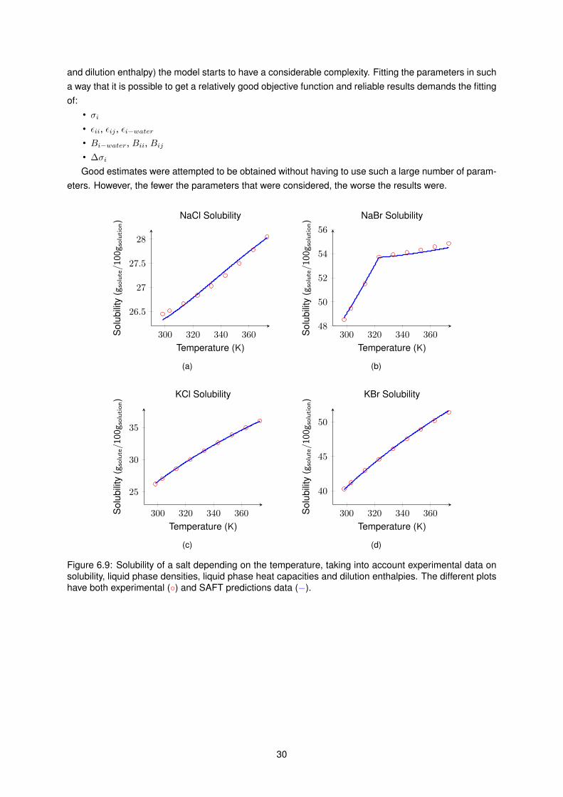
and dilution enthalpy) the model starts to have a considerable complexity. Fitting the parameters in sucha way that it is possible to get a relatively good objective function and reliable results demands the fittingof:

• σi• εii, εij , εi−water• Bi−water, Bii, Bij• ∆σi

Good estimates were attempted to be obtained without having to use such a large number of param-eters. However, the fewer the parameters that were considered, the worse the results were.

300 320 340 360

26.5

27

27.5

28

Temperature (K)

Sol

ubili

ty(g

solute/100g s

olution) NaCl Solubility

(a)

300 320 340 36048

50

52

54

56

Temperature (K)

Sol

ubili

ty(g

solute/100g s

olution) NaBr Solubility

(b)

300 320 340 360

25

30

35

Temperature (K)

Sol

ubili

ty(g

solute/100g s

olution) KCl Solubility

(c)

300 320 340 360

40

45

50

Temperature (K)

Sol

ubili

ty(g

solute/100g

solution) KBr Solubility

(d)

Figure 6.9: Solubility of a salt depending on the temperature, taking into account experimental data onsolubility, liquid phase densities, liquid phase heat capacities and dilution enthalpies. The different plotshave both experimental () and SAFT predictions data (−).

30

0 5 10500

1,000

1,500

2,000

Molality (molsolute/kgsolvent)

ρliqkg/m

3

NaCl ρliq

(a)

0 5 10500

1,000

1,500

2,000

Molality (molsolute/kgsolvent)

ρliqkg/m

3

NaBr ρliq

(b)

0 5 10500

1,000

1,500

2,000

Molality (molsolute/kgsolvent)

ρliqkg/m

3

KCl ρliq

(c)

0 5 10500

1,000

1,500

2,000

Molality (molsolute/kgsolvent)

ρliqkg/m

3

KBr ρliq

(d)

Figure 6.10: Liquid Phase Densities depending on molality, taking into account experimental data onsolubility, liquid phase densities, liquid phase heat capacities and dilution enthalpies. The different plotshave both experimental () and SAFT predictions data (−).

Both mean activity coefficients and osmotic coefficients can be predicted accurately (see AppendixC.4).

With respect to the liquid phase heat capacities, it was also possible to obtain the results in anaccurate way. As can be seen in Figure 6.11 all the experimental points are coincident with the onesprovided by the model. With only two values of liquid phase heat capacities, at two different molalities,the software is able to predict all the results for the remaining molality values.

31

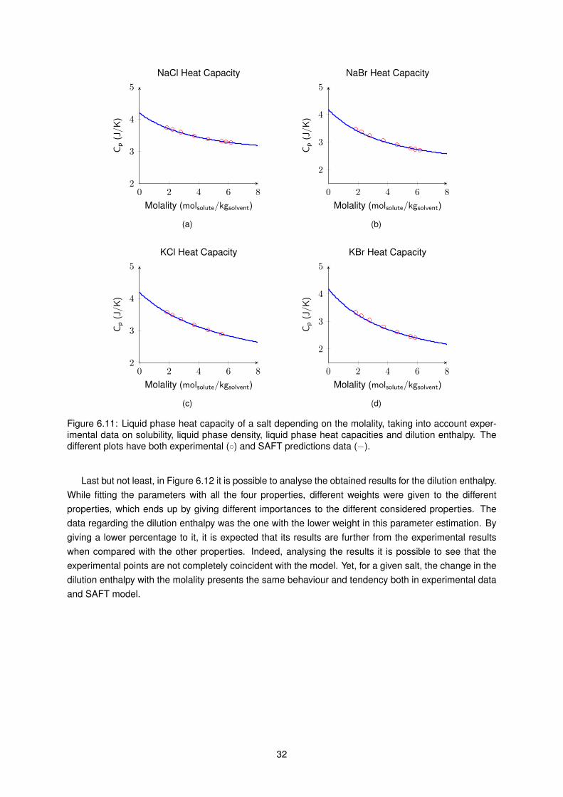
0 2 4 6 82

3

4

5

Molality (molsolute/kgsolvent)

Cp

(J/K

)

NaCl Heat Capacity

(a)

0 2 4 6 8

2

3

4

5

Molality (molsolute/kgsolvent)

Cp

(J/K

)

NaBr Heat Capacity

(b)

0 2 4 6 82

3

4

5

Molality (molsolute/kgsolvent)

Cp

(J/K

)

KCl Heat Capacity

(c)

0 2 4 6 8

2

3

4

5

Molality (molsolute/kgsolvent)

Cp

(J/K

)

KBr Heat Capacity

(d)

Figure 6.11: Liquid phase heat capacity of a salt depending on the molality, taking into account exper-imental data on solubility, liquid phase density, liquid phase heat capacities and dilution enthalpy. Thedifferent plots have both experimental () and SAFT predictions data (−).

Last but not least, in Figure 6.12 it is possible to analyse the obtained results for the dilution enthalpy.While fitting the parameters with all the four properties, different weights were given to the differentproperties, which ends up by giving different importances to the different considered properties. Thedata regarding the dilution enthalpy was the one with the lower weight in this parameter estimation. Bygiving a lower percentage to it, it is expected that its results are further from the experimental resultswhen compared with the other properties. Indeed, analysing the results it is possible to see that theexperimental points are not completely coincident with the model. Yet, for a given salt, the change in thedilution enthalpy with the molality presents the same behaviour and tendency both in experimental dataand SAFT model.

32

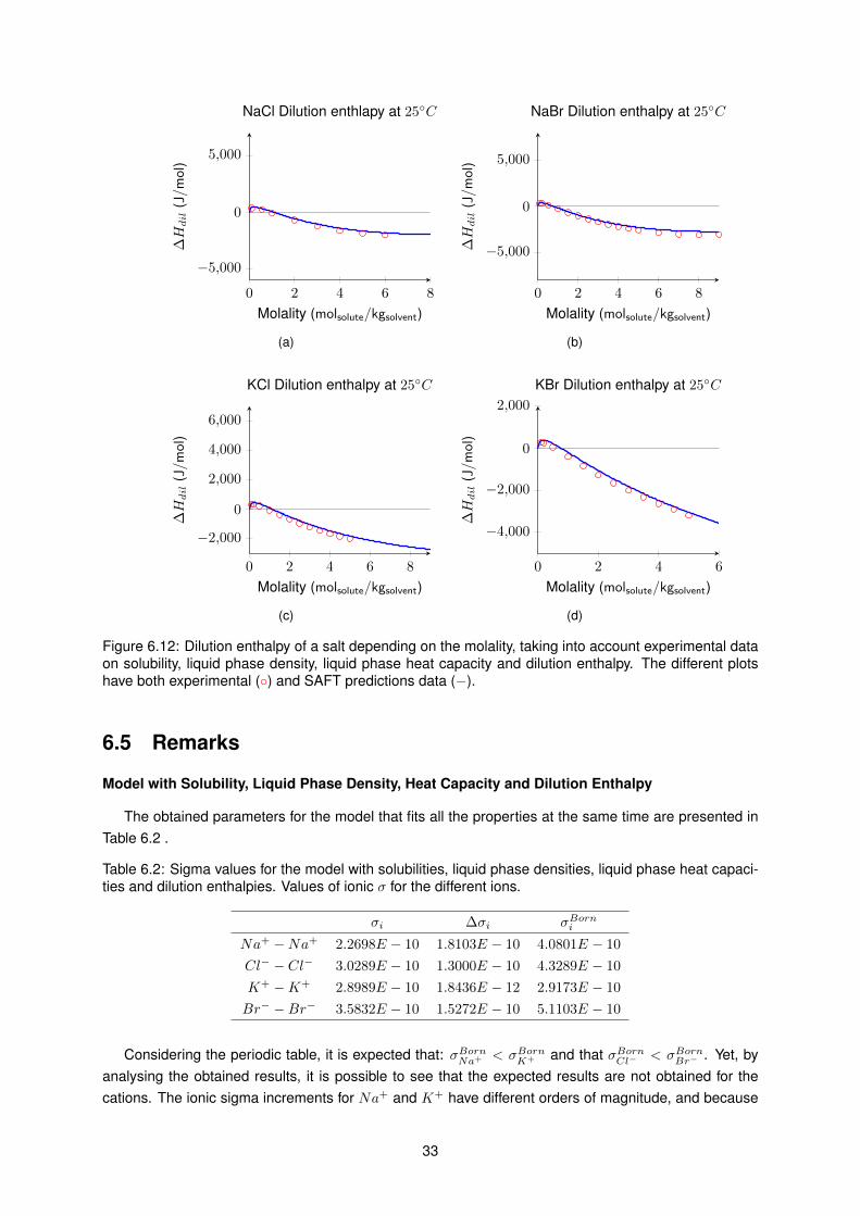
0 2 4 6 8

−5,000

0

5,000

Molality (molsolute/kgsolvent)

∆Hdil

(J/m

ol)

NaCl Dilution enthlapy at 25C

(a)

0 2 4 6 8

−5,000

0

5,000

Molality (molsolute/kgsolvent)

∆Hdil

(J/m

ol)

NaBr Dilution enthalpy at 25C

(b)

0 2 4 6 8

−2,000

0

2,000

4,000

6,000

Molality (molsolute/kgsolvent)

∆Hdil

(J/m

ol)

KCl Dilution enthalpy at 25C

(c)

0 2 4 6

−4,000

−2,000

0

2,000

Molality (molsolute/kgsolvent)

∆Hdil

(J/mol

)

KBr Dilution enthalpy at 25C

(d)

Figure 6.12: Dilution enthalpy of a salt depending on the molality, taking into account experimental dataon solubility, liquid phase density, liquid phase heat capacity and dilution enthalpy. The different plotshave both experimental () and SAFT predictions data (−).

6.5 Remarks

Model with Solubility, Liquid Phase Density, Heat Capacity and Dilution Enthalpy

The obtained parameters for the model that fits all the properties at the same time are presented inTable 6.2 .

Table 6.2: Sigma values for the model with solubilities, liquid phase densities, liquid phase heat capaci-ties and dilution enthalpies. Values of ionic σ for the different ions.

σi ∆σi σBorni

Na+ −Na+ 2.2698E − 10 1.8103E − 10 4.0801E − 10

Cl− − Cl− 3.0289E − 10 1.3000E − 10 4.3289E − 10

K+ −K+ 2.8989E − 10 1.8436E − 12 2.9173E − 10

Br− −Br− 3.5832E − 10 1.5272E − 10 5.1103E − 10

Considering the periodic table, it is expected that: σBornNa+ < σBornK+ and that σBornCl− < σBornBr− . Yet, byanalysing the obtained results, it is possible to see that the expected results are not obtained for thecations. The ionic sigma increments for Na+ and K+ have different orders of magnitude, and because

33

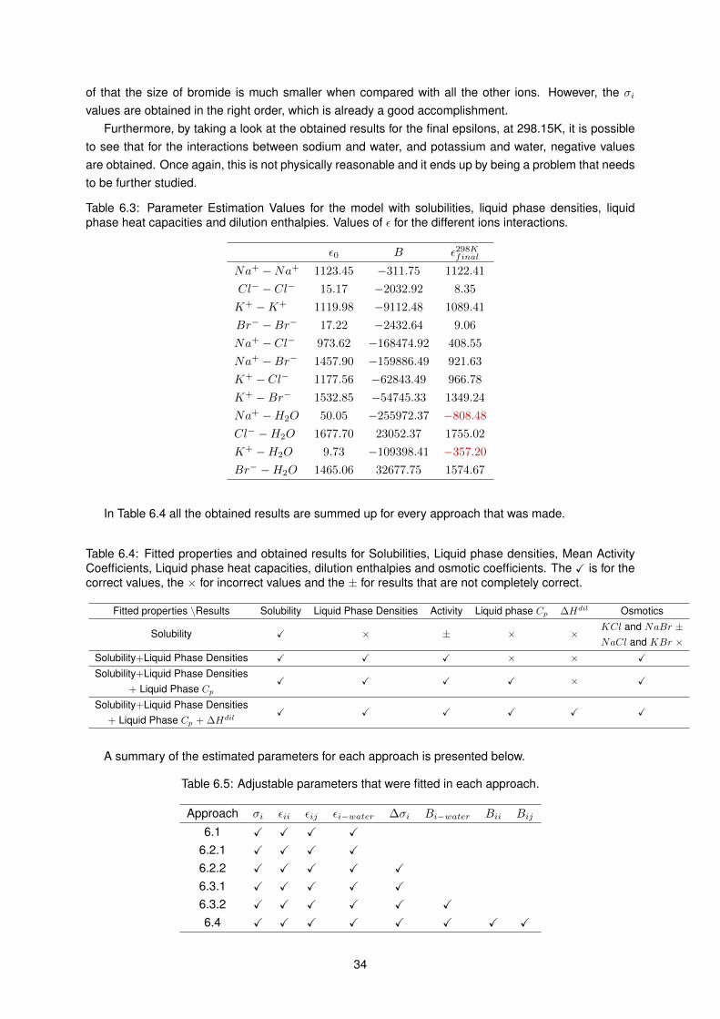
of that the size of bromide is much smaller when compared with all the other ions. However, the σi

values are obtained in the right order, which is already a good accomplishment.Furthermore, by taking a look at the obtained results for the final epsilons, at 298.15K, it is possible

to see that for the interactions between sodium and water, and potassium and water, negative valuesare obtained. Once again, this is not physically reasonable and it ends up by being a problem that needsto be further studied.

Table 6.3: Parameter Estimation Values for the model with solubilities, liquid phase densities, liquidphase heat capacities and dilution enthalpies. Values of ε for the different ions interactions.

ε0 B ε298Kfinal

Na+ −Na+ 1123.45 −311.75 1122.41

Cl− − Cl− 15.17 −2032.92 8.35

K+ −K+ 1119.98 −9112.48 1089.41

Br− −Br− 17.22 −2432.64 9.06

Na+ − Cl− 973.62 −168474.92 408.55

Na+ −Br− 1457.90 −159886.49 921.63

K+ − Cl− 1177.56 −62843.49 966.78

K+ −Br− 1532.85 −54745.33 1349.24

Na+ −H2O 50.05 −255972.37 −808.48

Cl− −H2O 1677.70 23052.37 1755.02

K+ −H2O 9.73 −109398.41 −357.20

Br− −H2O 1465.06 32677.75 1574.67

In Table 6.4 all the obtained results are summed up for every approach that was made.

Table 6.4: Fitted properties and obtained results for Solubilities, Liquid phase densities, Mean ActivityCoefficients, Liquid phase heat capacities, dilution enthalpies and osmotic coefficients. The X is for thecorrect values, the × for incorrect values and the ± for results that are not completely correct.

Fitted properties \Results Solubility Liquid Phase Densities Activity Liquid phase Cp ∆Hdil Osmotics

Solubility X × ± × ×KCl and NaBr ±NaCl and KBr ×

Solubility+Liquid Phase Densities X X X × × X

Solubility+Liquid Phase Densities+ Liquid Phase Cp

X X X X × X

Solubility+Liquid Phase Densities+ Liquid Phase Cp + ∆Hdil

X X X X X X

A summary of the estimated parameters for each approach is presented below.

Table 6.5: Adjustable parameters that were fitted in each approach.

Approach σi εii εij εi−water ∆σi Bi−water Bii Bij

6.1 X X X X

6.2.1 X X X X

6.2.2 X X X X X

6.3.1 X X X X X

6.3.2 X X X X X X

6.4 X X X X X X X X

34

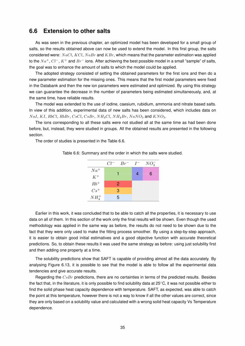
6.6 Extension to other salts

As was seen in the previous chapter, an optimized model has been developed for a small group ofsalts, so the results obtained above can now be used to extend the model. In this first group, the saltsconsidered were: NaCl, KCl, NaBr and KBr, which means that the parameter estimation was appliedto the Na+, Cl−, K+ and Br− ions. After achieving the best possible model in a small ”sample” of salts,the goal was to enhance the amount of salts to which the model could be applied.

The adopted strategy consisted of setting the obtained parameters for the first ions and then do anew parameter estimation for the missing ones. This means that the first model parameters were fixedin the Databank and then the new ion parameters were estimated and optimized. By using this strategywe can guarantee the decrease in the number of parameters being estimated simultaneously, and, atthe same time, have reliable results.

The model was extended to the use of iodine, caesium, rubidium, ammonia and nitrate based salts.In view of this addition, experimental data of new salts has been considered, which includes data onNaI, KI, RbCl, RbBr, CsCl, CsBr, NH4Cl, NH4Br, NaNO3 and KNO3.

The ions corresponding to all these salts were not studied all at the same time as had been donebefore, but, instead, they were studied in groups. All the obtained results are presented in the followingsection.

The order of studies is presented in the Table 6.6.

Table 6.6: Summary and the order in which the salts were studied.

Cl− Br− I− NO−3

Na+

K+1 4 6

Rb+ 2Cs+ 3NH+

4 5

Earlier in this work, it was concluded that to be able to catch all the properties, it is necessary to usedata on all of them. In this section of the work only the final results will be shown. Even though the usedmethodology was applied in the same way as before, the results do not need to be shown due to thefact that they were only used to make the fitting process smoother. By using a step-by-step approach,it is easier to obtain good initial estimatives and a good objective function with accurate theoreticalpredictions. So, to obtain these results it was used the same strategy as before: using just solubility firstand then adding one property at a time.

The solubility predictions show that SAFT is capable of providing almost all the data accurately. Byanalysing Figure 6.13, it is possible to see that the model is able to follow all the experimental datatendencies and give accurate results.

Regarding the CsBr predictions, there are no certainties in terms of the predicted results. Besidesthe fact that, in the literature, it is only possible to find solubility data at 25C, it was not possible either tofind the solid phase heat capacity dependence with temperature. SAFT, as expected, was able to catchthe point at this temperature, however there is not a way to know if all the other values are correct, sincethey are only based on a solubility value and calculated with a wrong solid heat capacity Vs Temperaturedependence.

35

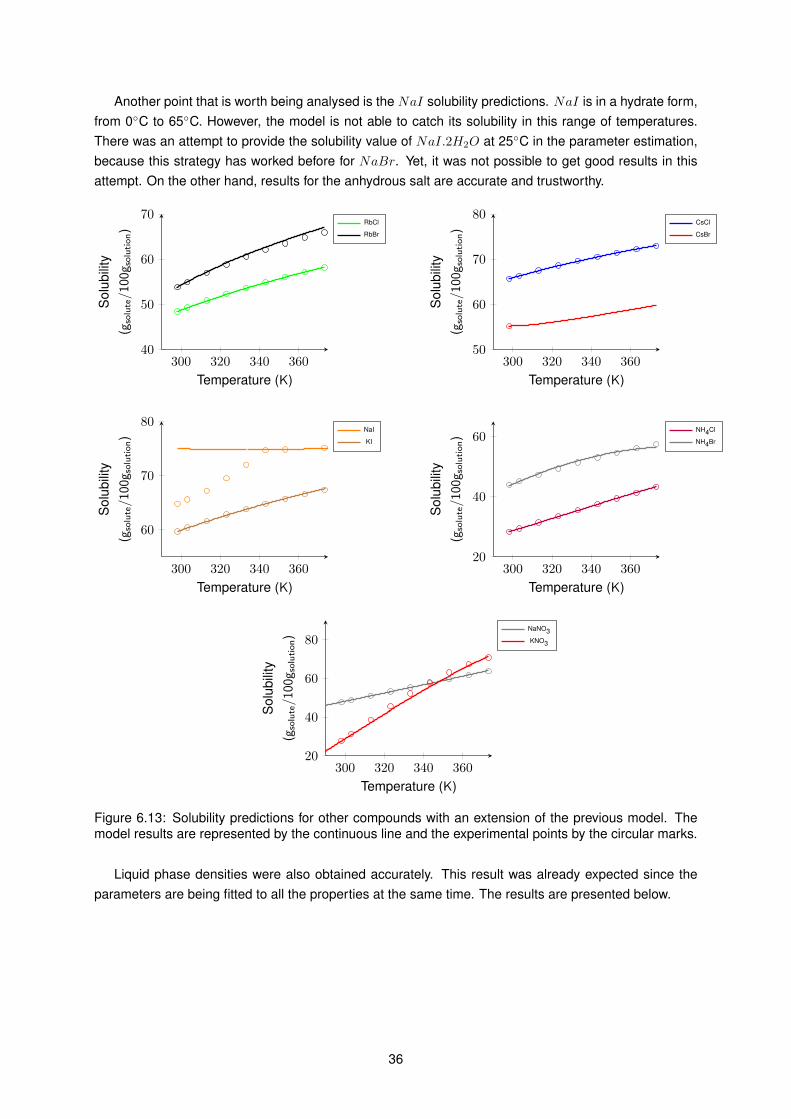
Another point that is worth being analysed is the NaI solubility predictions. NaI is in a hydrate form,from 0C to 65C. However, the model is not able to catch its solubility in this range of temperatures.There was an attempt to provide the solubility value of NaI.2H2O at 25C in the parameter estimation,because this strategy has worked before for NaBr. Yet, it was not possible to get good results in thisattempt. On the other hand, results for the anhydrous salt are accurate and trustworthy.

300 320 340 36040

50

60

70

Temperature (K)

Sol

ubili

ty(g

solute/100g s

olution)

RbCl

RbBr

300 320 340 36050

60

70

80

Temperature (K)

Sol

ubili

ty(g

solute/100g s

olution)

CsCl

CsBr

300 320 340 360

60

70

80

Temperature (K)

Sol

ubili

ty(g

solute/100g s

olution)

NaI

KI

300 320 340 36020

40

60

Temperature (K)

Sol

ubili

ty(g

solute/100g s

olution)

NH4Cl

NH4Br

300 320 340 36020

40

60

80

Temperature (K)

Sol

ubili

ty(g

solute/100g s

olution)

NaNO3KNO3

Figure 6.13: Solubility predictions for other compounds with an extension of the previous model. Themodel results are represented by the continuous line and the experimental points by the circular marks.

Liquid phase densities were also obtained accurately. This result was already expected since theparameters are being fitted to all the properties at the same time. The results are presented below.

36

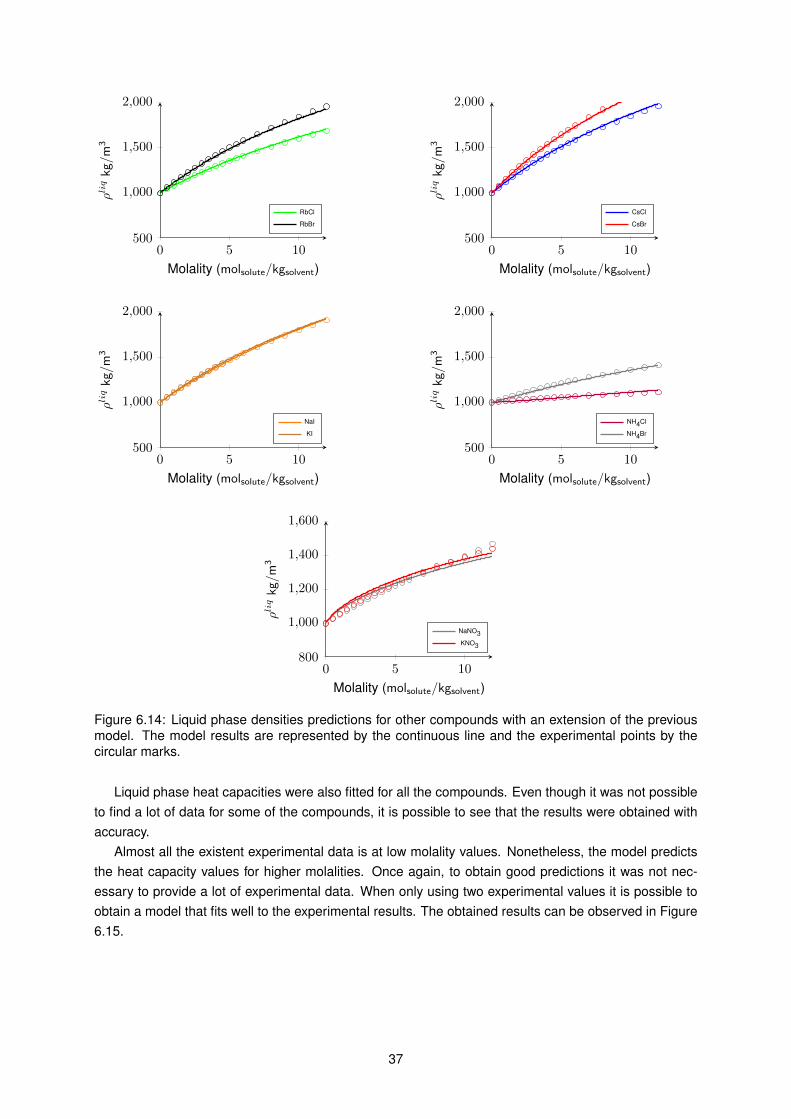
0 5 10500

1,000

1,500

2,000

Molality (molsolute/kgsolvent)

ρliqkg/m

3

RbCl

RbBr

0 5 10500

1,000

1,500

2,000

Molality (molsolute/kgsolvent)

ρliqkg/m

3

CsCl

CsBr

0 5 10500

1,000

1,500

2,000

Molality (molsolute/kgsolvent)

ρliqkg/m

3

NaI

KI

0 5 10500

1,000

1,500

2,000

Molality (molsolute/kgsolvent)

ρliqkg/m

3NH4Cl

NH4Br

0 5 10800

1,000

1,200

1,400

1,600

Molality (molsolute/kgsolvent)

ρliqkg/m

3

NaNO3KNO3

Figure 6.14: Liquid phase densities predictions for other compounds with an extension of the previousmodel. The model results are represented by the continuous line and the experimental points by thecircular marks.

Liquid phase heat capacities were also fitted for all the compounds. Even though it was not possibleto find a lot of data for some of the compounds, it is possible to see that the results were obtained withaccuracy.

Almost all the existent experimental data is at low molality values. Nonetheless, the model predictsthe heat capacity values for higher molalities. Once again, to obtain good predictions it was not nec-essary to provide a lot of experimental data. When only using two experimental values it is possible toobtain a model that fits well to the experimental results. The obtained results can be observed in Figure6.15.

37

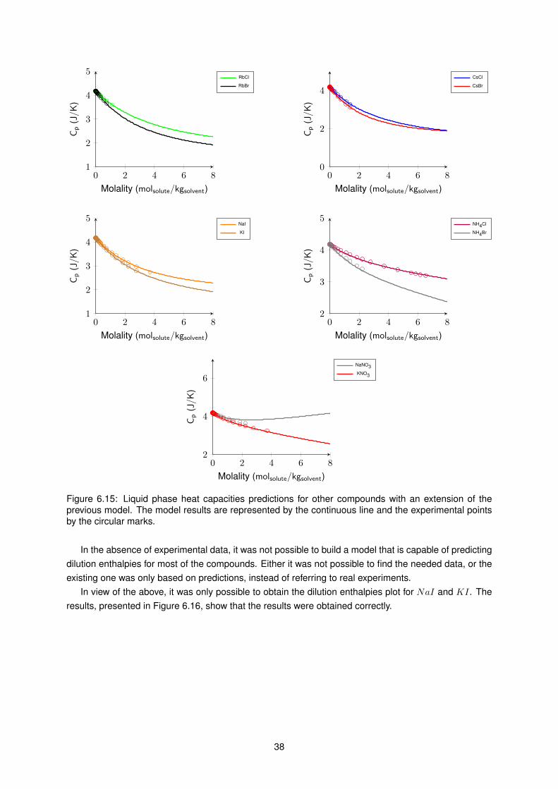
0 2 4 6 81

2

3

4

5

Molality (molsolute/kgsolvent)

Cp

(J/K

)RbCl

RbBr

0 2 4 6 80

2

4

Molality (molsolute/kgsolvent)

Cp

(J/K

)

CsCl

CsBr

0 2 4 6 81

2

3

4

5

Molality (molsolute/kgsolvent)

Cp

(J/K

)

NaI

KI

0 2 4 6 82

3

4

5

Molality (molsolute/kgsolvent)

Cp

(J/K

)

NH4Cl

NH4Br

0 2 4 6 82

4

6

Molality (molsolute/kgsolvent)

Cp

(J/K

)

NaNO3KNO3

Figure 6.15: Liquid phase heat capacities predictions for other compounds with an extension of theprevious model. The model results are represented by the continuous line and the experimental pointsby the circular marks.

In the absence of experimental data, it was not possible to build a model that is capable of predictingdilution enthalpies for most of the compounds. Either it was not possible to find the needed data, or theexisting one was only based on predictions, instead of referring to real experiments.

In view of the above, it was only possible to obtain the dilution enthalpies plot for NaI and KI. Theresults, presented in Figure 6.16, show that the results were obtained correctly.

38

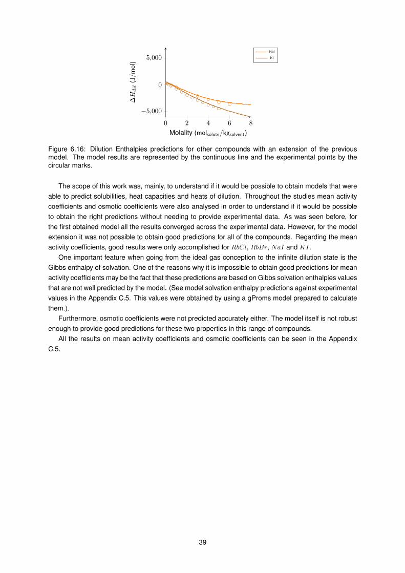
0 2 4 6 8

−5,000

0

5,000

Molality (molsolute/kgsolvent)∆Hdil

(J/m

ol)

NaI

KI

Figure 6.16: Dilution Enthalpies predictions for other compounds with an extension of the previousmodel. The model results are represented by the continuous line and the experimental points by thecircular marks.

The scope of this work was, mainly, to understand if it would be possible to obtain models that wereable to predict solubilities, heat capacities and heats of dilution. Throughout the studies mean activitycoefficients and osmotic coefficients were also analysed in order to understand if it would be possibleto obtain the right predictions without needing to provide experimental data. As was seen before, forthe first obtained model all the results converged across the experimental data. However, for the modelextension it was not possible to obtain good predictions for all of the compounds. Regarding the meanactivity coefficients, good results were only accomplished for RbCl, RbBr, NaI and KI.

One important feature when going from the ideal gas conception to the infinite dilution state is theGibbs enthalpy of solvation. One of the reasons why it is impossible to obtain good predictions for meanactivity coefficients may be the fact that these predictions are based on Gibbs solvation enthalpies valuesthat are not well predicted by the model. (See model solvation enthalpy predictions against experimentalvalues in the Appendix C.5. This values were obtained by using a gProms model prepared to calculatethem.).

Furthermore, osmotic coefficients were not predicted accurately either. The model itself is not robustenough to provide good predictions for these two properties in this range of compounds.

All the results on mean activity coefficients and osmotic coefficients can be seen in the AppendixC.5.

39

40

Chapter 7

Conclusions

The conventional strategy to determine SAFT parameters for electrolyte systems is usually basedon regressing a combination of properties including activity coefficients, osmotic coefficients, vapourpressures and liquid phase densities. This study demonstrates that this methodology does not guaranteethat the obtained parameters can be used to predict calorific properties, such as heat capacities andheats of dilution. We propose that calorific properties should always be included in the regression ofparameters when they are available. The main conclusions of this study are:

• It is possible to fit the parameters to solubilities and to obtain accurate theoretical predictions for it;

• If one wants to obtain accurate computations on solubilities, liquid phase heat capacities anddilution enthalpies it is necessary to fit to every property;

• In order to obtain accurate predictions, it is not necessary to use a lot of experimental data. Withonly two points at different molalities, it is possible to obtain good results for liquid phase heatcapacities, liquid phase densities and dilution enthalpies;

• The first developed model for NaCl, NaBr, KCl and KBr is able to provide accurate results formean activity coefficients and osmotic coefficients without them being included in the fit;

• The negative values of the cross ion-water dispersion energy might be due to some shortcomingsof the Born contribution which need to be compensated ;

• A sequential fit of different salts is a suitable approach to develop parameters from ionic groups;

• NO –3 and NH +

4 are not easy to model, mainly for two reasons:

- Both ions are not spherical, especially the nitrate. Their shape factor was considered andset as 1 and this may lead to difficulties with its fitting;

- One of the data needed for the parameters fitting is the ideal gas heat capacity. Formonoatomic species this value is known and set as 20.8. However, neither of these two species ismonoatomic, and, because of that, their ideal gas heat capacity has a different value (which wasnot considered in the fitting.);

41

42

Bibliography

[1] J. Pamies Corominas, “Bulk and interfacial properties of chain fluids: a molecular modelling ap-proach,” Ph.D. dissertation, 2004.

[2] V. Papaioannou, “A molecular-based group contribution equation of state for the description offluid phase behaviour and thermodynamic derivative properties of mixtures ( SAFT- γ Mie ),” no.December, 2012.

[3] G. M. Kontogeorgis, B. Maribo-Mogensen, and K. Thomsen, “The Debye-Huckel theory and itsimportance in modeling electrolyte solutions,” Fluid Phase Equilibria, 2018. [Online]. Available:http://linkinghub.elsevier.com/retrieve/pii/S0378381218300074

[4] J. M. Schreckenberg, S. Dufal, A. J. Haslam, C. S. Adjiman, G. Jackson, and A. Galindo, “Modellingof the thermodynamic and solvation properties of electrolyte solutions with the statistical associatingfluid theory for potentials of variable range,” Molecular Physics, vol. 112, 2014.

[5] D. K. Eriksen, G. Lazarou, A. Galindo, G. Jackson, C. S. Adjiman, and A. J. Haslam, “Develop-ment of intermolecular potential models for electrolyte solutions using an electrolyte SAFT-VR Mieequation of state,” Molecular Physics, vol. 114, no. 18, 2016.

[6] B. Maribo-mogensen, Development of an Electrolyte CPA Equation of state for Ap-plications in the Petroleum and Chemical Industries Equation of State for Ap-plications in the, 2014, no. June. [Online]. Available: http://orbit.dtu.dk/en/persons/bjoern-maribomogensen(597d1611-cf48-444c-a982-52766587bce5)/publications.html

[7] S. Dufal, “Development and application of advanced thermodynamic molecular description for com-plex reservoir fluids containing carbon dioxide and brines,” 2013.

[8] M. A. Selam, I. G. Economou, and M. Castier, “A thermodynamic model for strong aqueous elec-trolytes based on the eSAFT-VR Mie equation of state,” Fluid Phase Equilibria, vol. 464, pp. 47–63,2018.

[9] T. Lafitte, V. Papaioannou, S. Dufal, and C. C. Pantelides, “A general framework for solid-liquidequilibria in pharmaceutical systems.”

[10] D. D. Wagman, W. H. Evans, V. B. Parker, R. H. Schumm, I. Halow, S. M. Bailey, K. L. Churney, andR. L. Nuttall, “The NBS Tables of Chemical Thermodynamic Properties,” 1982.

[11] T. Lafitte, “Technical Training – gSAFT Session,” pp. 1–24, 2017.

[12] V. Papaioannou, T. Lafitte, C. Avendano, C. S. Adjiman, G. Jackson, E. A. Muller, and A. Galindo,“Group contribution methodology based on the statistical associating fluid theory for heteronuclearmolecules formed from Mie segments,” Journal of Chemical Physics, vol. 140, no. 5, 2014.

43

[13] T. Lafitte, A. Apostolakou, C. Avendano, A. Galindo, C. S. Adjiman, E. A. Muller, and G. Jack-son, “Accurate statistical associating fluid theory for chain molecules formed from Mie segments,”Journal of Chemical Physics, vol. 139, no. 15, 2013.

[14] “NIST Chemistry WebBook.” [Online]. Available: https://webbook.nist.gov/chemistry/

[15] R. H. Perry and D. W. Green, Perry’s Chemical Engineers’ Handbook, 2008, vol. 1.

[16] A. Seidell, Solubilities of Inorganic and Organic Compounds: A compilation of quantitative solubiltydata from the periodical literature, 2nd ed., New York, 1919.

[17] B. S. Krumgalz, “Temperature dependence of mineral solubility in water. Part I. Alkaline andAlkaline earth chlorides,” Journal of Physical and Chemical Reference Data, vol. 46, 2017.[Online]. Available: http://dx.doi.org/10.1063/1.5010290

[18] S. P. Pinho and E. A. Macedo, “Solubility of NaCl, NaBr, and KCl in water, methanol, ethanol, andtheir mixed solvents,” Journal of Chemical and Engineering Data, vol. 50, no. 1, pp. 29–32, 2005.

[19] D. Lide, “Aqueous Solubility of Inorganic Compounds at Various Temperatures,” CRCHandbook of Chemistry and Physics, 2005. [Online]. Available: papers2://publication/uuid/55E853FE-9E62-4EEC-97D7-AFAB12AA3361

[20] J. W. Lorimer, M. Salomon, and C. L. Young, Solubility data series: Alkali metal and ammoniumchlorides in water and heavy water (binary systems), 1991, vol. 47.

[21] B. S. Krumgalz, R. Pogorelsky, and K. S. Pitzer, “Volumetric Properties of Single Aqueous Elec-trolytes from Zero to Saturation Concentration at 298.15K Represented by Pitzer’s Ion-InteractionEquations,” J.Phys.Chem, vol. 25, no. 2, p. 663, 1995.

[22] V. B. Parker, “Thermal Properties of Aqueoues Uni-univalent Electrolytes,” pp. 1–66, 1965.

[23] W. J.Hammer and Y.-C. Wu, “Osmotic Coefficients and Mean Activity Coefficients of Uni-ValentElectrolytes in water at 25 Degrees,” J. Phys. Chem., vol. 1, no. 4, p. 1047, 1972.

[24] “Heat of Solution.” [Online]. Available: https://courses.lumenlearning.com/introchem/chapter/heat-of-solution/

[25] W. R. Fawcett, “Thermodynamic Parameters for the Solvation of Monatomic Ions in Water,” TheJournal of Physical Chemistry B, vol. 103, no. 50, pp. 11 181–11 185, 1999. [Online]. Available:http://dx.doi.org/10.1021/jp991802n%5Cnhttp://pubs.acs.org/doi/abs/10.1021/jp991802n

44

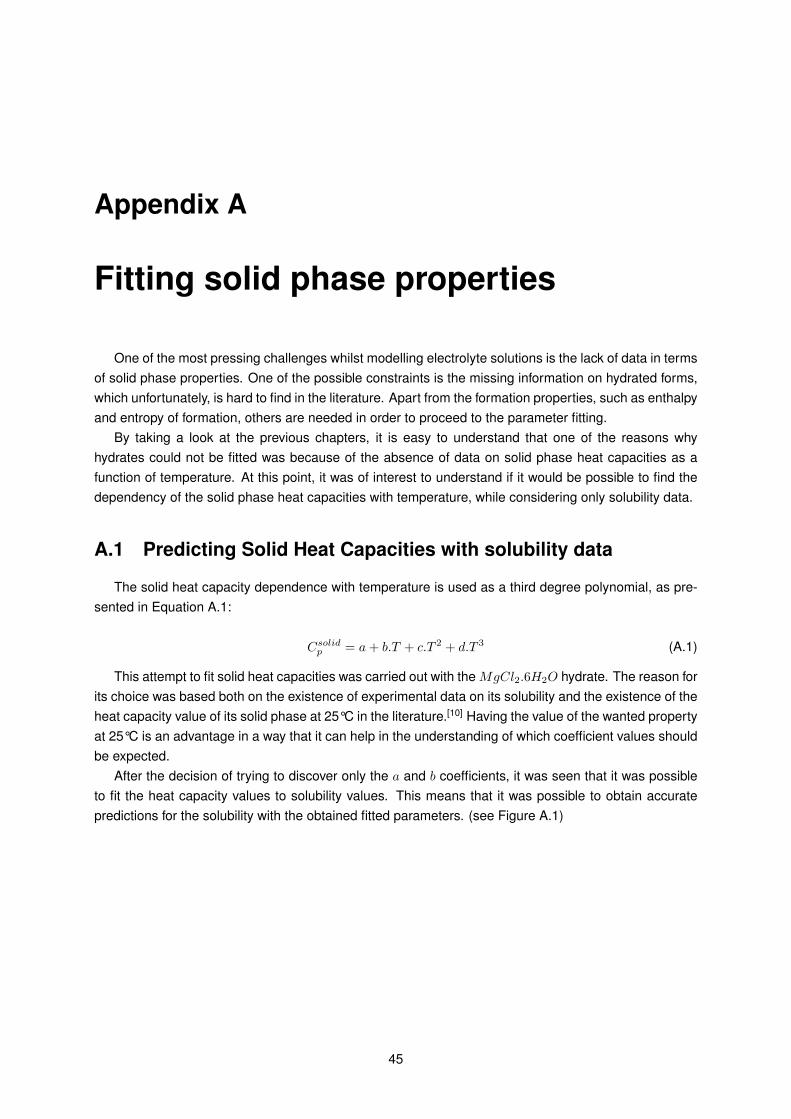
Appendix A

Fitting solid phase properties

One of the most pressing challenges whilst modelling electrolyte solutions is the lack of data in termsof solid phase properties. One of the possible constraints is the missing information on hydrated forms,which unfortunately, is hard to find in the literature. Apart from the formation properties, such as enthalpyand entropy of formation, others are needed in order to proceed to the parameter fitting.

By taking a look at the previous chapters, it is easy to understand that one of the reasons whyhydrates could not be fitted was because of the absence of data on solid phase heat capacities as afunction of temperature. At this point, it was of interest to understand if it would be possible to find thedependency of the solid phase heat capacities with temperature, while considering only solubility data.

A.1 Predicting Solid Heat Capacities with solubility data

The solid heat capacity dependence with temperature is used as a third degree polynomial, as pre-sented in Equation A.1:

Csolidp = a+ b.T + c.T 2 + d.T 3 (A.1)

This attempt to fit solid heat capacities was carried out with the MgCl2.6H2O hydrate. The reason forits choice was based both on the existence of experimental data on its solubility and the existence of theheat capacity value of its solid phase at 25°C in the literature.[10] Having the value of the wanted propertyat 25°C is an advantage in a way that it can help in the understanding of which coefficient values shouldbe expected.

After the decision of trying to discover only the a and b coefficients, it was seen that it was possibleto fit the heat capacity values to solubility values. This means that it was possible to obtain accuratepredictions for the solubility with the obtained fitted parameters. (see Figure A.1)

45

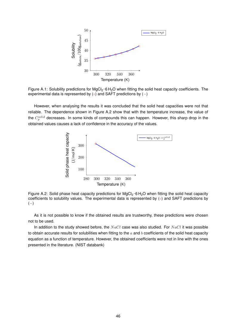
300 320 340 36030

35

40

45

50

Temperature (K)

Sol

ubili

ty(g

solute/100g s

olution)

MgCl2 · 6 H2O

Figure A.1: Solubility predictions for MgCl2 · 6 H2O when fitting the solid heat capacity coefficients. Theexperimental data is represented by () and SAFT predictions by (−)

However, when analysing the results it was concluded that the solid heat capacities were not thatreliable. The dependence shown in Figure A.2 show that with the temperature increase, the value ofthe Csolidp decreases. In some kinds of compounds this can happen. However, this sharp drop in theobtained values causes a lack of confidence in the accuracy of the values.

280 300 320 340 360

100

200

300

Temperature (K)

Sol

idph

ase

heat

capa

city

(J/m

olK

)

MgCl2 · 6 H2O :Csolidp

Figure A.2: Solid phase heat capacity predictions for MgCl2 · 6 H2O when fitting the solid heat capacitycoefficients to solubility values. The experimental data is represented by () and SAFT predictions by(−)

As it is not possible to know if the obtained results are trustworthy, these predictions were chosennot to be used.

In addition to the study showed before, the NaCl case was also studied. For NaCl it was possibleto obtain accurate results for solubilities when fitting to the a and b coefficients of the solid heat capacityequation as a function of temperature. However, the obtained coefficients were not in line with the onespresented in the literature. (NIST databank)

46

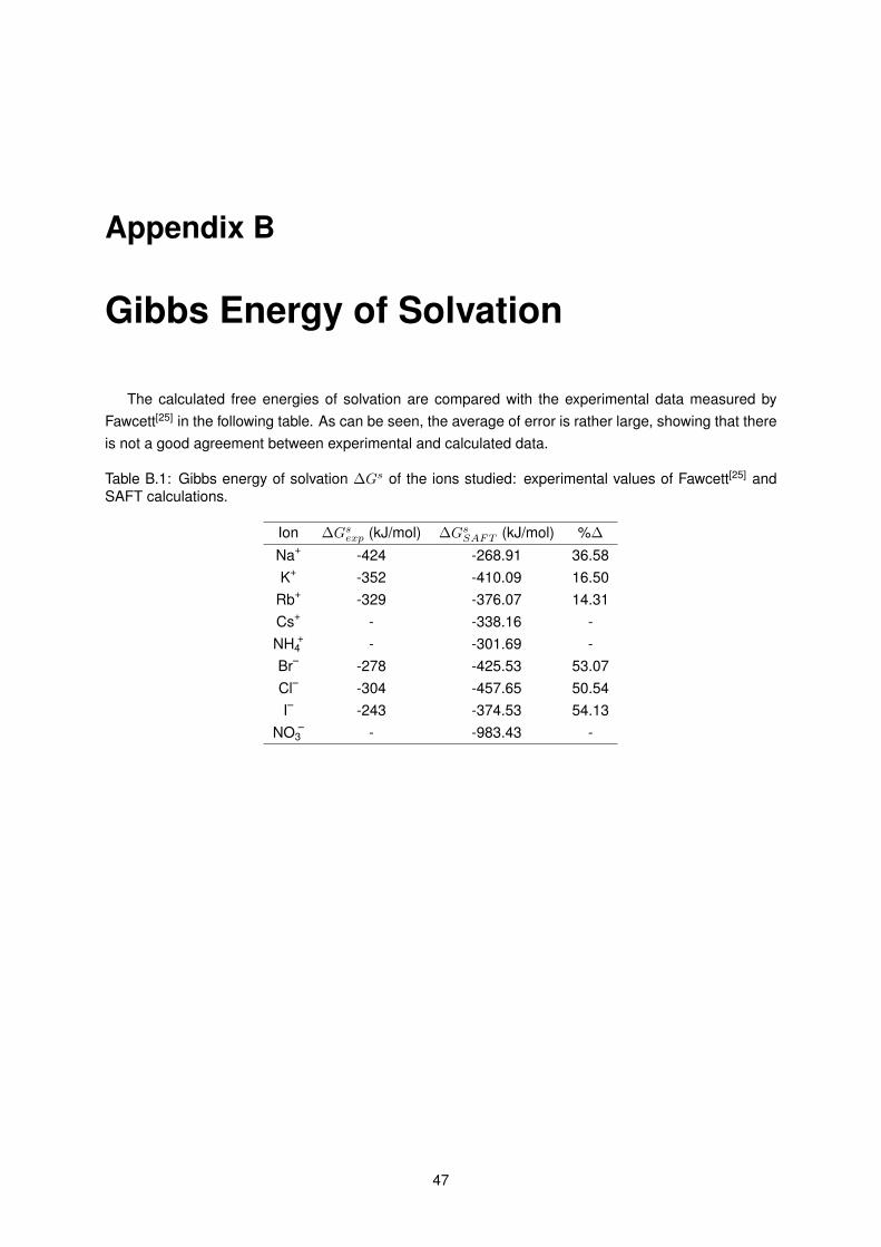
Appendix B

Gibbs Energy of Solvation

The calculated free energies of solvation are compared with the experimental data measured byFawcett[25] in the following table. As can be seen, the average of error is rather large, showing that thereis not a good agreement between experimental and calculated data.

Table B.1: Gibbs energy of solvation ∆Gs of the ions studied: experimental values of Fawcett[25] andSAFT calculations.

Ion ∆Gsexp (kJ/mol) ∆GsSAFT (kJ/mol) %∆

Na+ -424 -268.91 36.58K+ -352 -410.09 16.50

Rb+ -329 -376.07 14.31Cs+ - -338.16 -NH +

4 - -301.69 -Br– -278 -425.53 53.07Cl– -304 -457.65 50.54I– -243 -374.53 54.13

NO –3 - -983.43 -

47

48

Appendix C

Parameter Estimation Results

C.1 Estimation using solubility

C.1.1 Liquid Phase Density results

0 5 10500

1,000

1,500

2,000

Molality (molsolute/kgsolvent)

ρliqkg/m

3

NaCl ρliq

(a)

0 5 10500

1,000

1,500

2,000

Molality (molsolute/kgsolvent)

ρliqkg/m

3

NaBr ρliq

(b)

0 5 10500

1,000

1,500

2,000

Molality (molsolute/kgsolvent)

ρliqkg/m

3

KCl ρliq

(c)

0 5 10500

1,000

1,500

2,000

Molality (molsolute/kgsolvent)

ρliqkg/m

3

KBr ρliq

(d)

Figure C.1: Liquid phase density depending on the molality, taking into account only experimental dataon solubility. The different plots have both experimental () and SAFT predictions data (−).

49

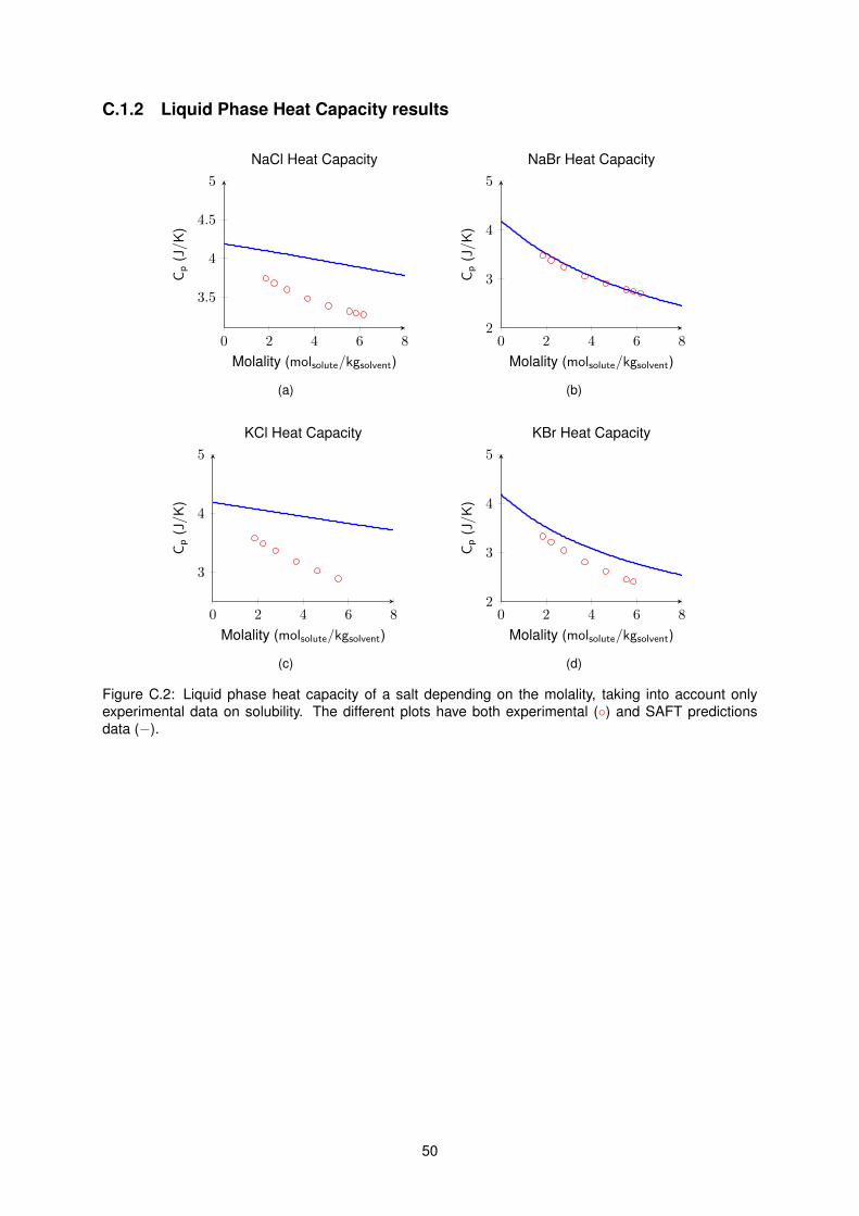
C.1.2 Liquid Phase Heat Capacity results

0 2 4 6 8

3.5

4

4.5

5

Molality (molsolute/kgsolvent)

Cp

(J/K

)NaCl Heat Capacity

(a)

0 2 4 6 82

3

4

5

Molality (molsolute/kgsolvent)

Cp

(J/K

)

NaBr Heat Capacity

(b)

0 2 4 6 8

3

4

5

Molality (molsolute/kgsolvent)

Cp

(J/K

)

KCl Heat Capacity

(c)

0 2 4 6 82

3

4

5

Molality (molsolute/kgsolvent)

Cp

(J/K

)

KBr Heat Capacity

(d)

Figure C.2: Liquid phase heat capacity of a salt depending on the molality, taking into account onlyexperimental data on solubility. The different plots have both experimental () and SAFT predictionsdata (−).

50

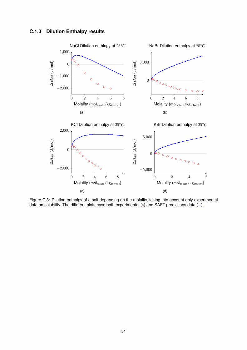
C.1.3 Dilution Enthalpy results

0 2 4 6 8

−2,000

−1,000

0

1,000

Molality (molsolute/kgsolvent)

∆Hdil

(J/m

ol)

NaCl Dilution enthlapy at 25C

(a)

0 2 4 6 8

0

5,000

Molality (molsolute/kgsolvent)

∆Hdil

(J/mol

)

NaBr Dilution enthalpy at 25C

(b)

0 2 4 6 8

−2,000

0

2,000

Molality (molsolute/kgsolvent)

∆Hdil

(J/m

ol)

KCl Dilution enthalpy at 25C

(c)

0 2 4 6

−5,000

0

5,000

Molality (molsolute/kgsolvent)

∆Hdil

(J/mol

)

KBr Dilution enthalpy at 25C

(d)

Figure C.3: Dilution enthalpy of a salt depending on the molality, taking into account only experimentaldata on solubility. The different plots have both experimental () and SAFT predictions data (−).

51

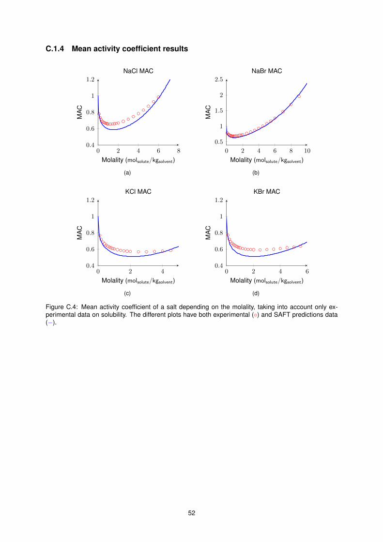
C.1.4 Mean activity coefficient results

0 2 4 6 80.4

0.6

0.8

1

1.2

Molality (molsolute/kgsolvent)

MA

CNaCl MAC

(a)

0 2 4 6 8 10

0.5

1

1.5

2

2.5

Molality (molsolute/kgsolvent)

MA

C

NaBr MAC

(b)

0 2 40.4

0.6

0.8

1

1.2

Molality (molsolute/kgsolvent)

MA

C

KCl MAC

(c)

0 2 4 60.4

0.6

0.8

1

1.2

Molality (molsolute/kgsolvent)

MA

C

KBr MAC

(d)

Figure C.4: Mean activity coefficient of a salt depending on the molality, taking into account only ex-perimental data on solubility. The different plots have both experimental () and SAFT predictions data(−).

52

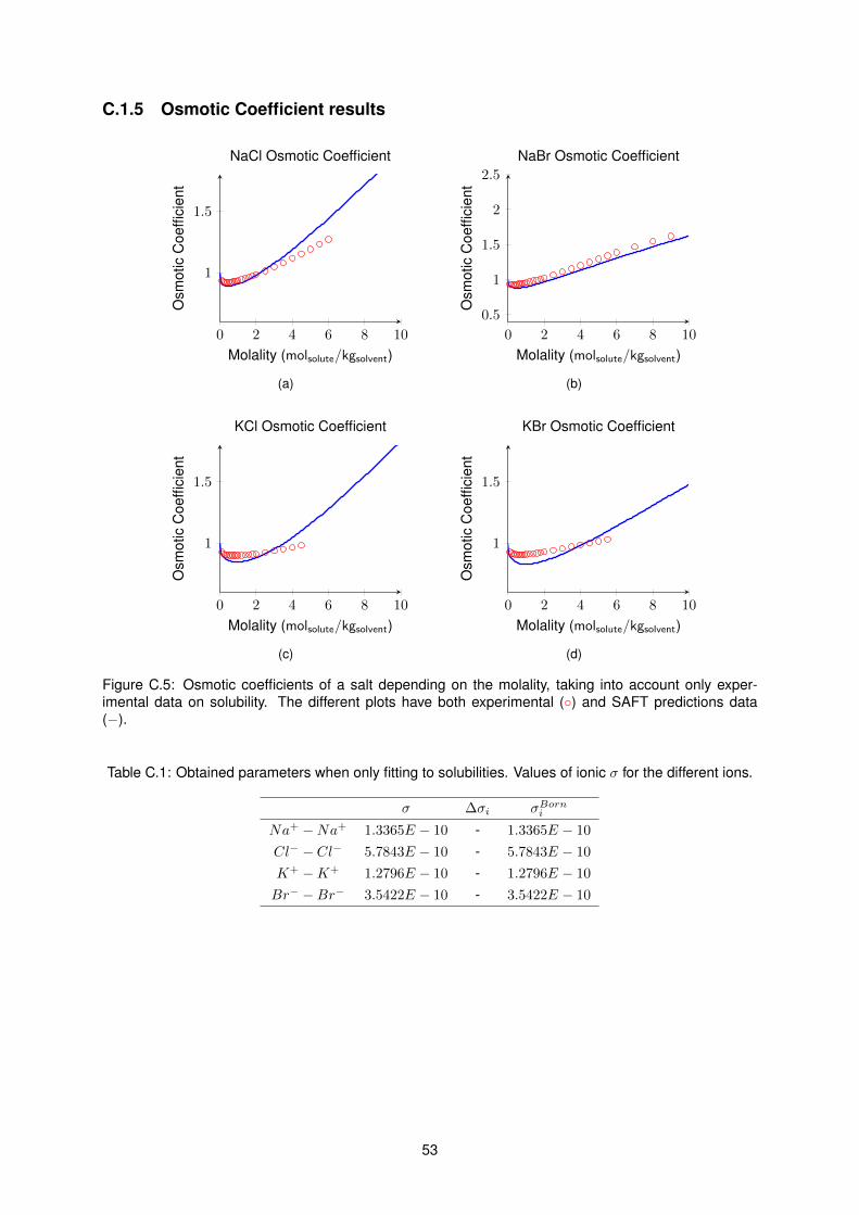
C.1.5 Osmotic Coefficient results

0 2 4 6 8 10

1

1.5

Molality (molsolute/kgsolvent)

Osm

otic

Coe

ffici

ent

NaCl Osmotic Coefficient

(a)

0 2 4 6 8 10

0.5

1

1.5

2

2.5

Molality (molsolute/kgsolvent)

Osm

otic

Coe

ffici

ent

NaBr Osmotic Coefficient

(b)

0 2 4 6 8 10

1

1.5

Molality (molsolute/kgsolvent)

Osm

otic

Coe

ffici

ent

KCl Osmotic Coefficient

(c)

0 2 4 6 8 10

1

1.5

Molality (molsolute/kgsolvent)

Osm

otic

Coe

ffici

ent

KBr Osmotic Coefficient

(d)

Figure C.5: Osmotic coefficients of a salt depending on the molality, taking into account only exper-imental data on solubility. The different plots have both experimental () and SAFT predictions data(−).

Table C.1: Obtained parameters when only fitting to solubilities. Values of ionic σ for the different ions.

σ ∆σi σBorni

Na+ −Na+ 1.3365E − 10 - 1.3365E − 10

Cl− − Cl− 5.7843E − 10 - 5.7843E − 10

K+ −K+ 1.2796E − 10 - 1.2796E − 10

Br− −Br− 3.5422E − 10 - 3.5422E − 10

53

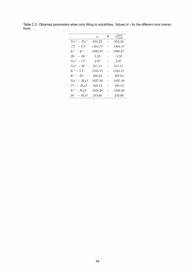
Table C.2: Obtained parameters when only fitting to solubilities. Values of ε for the different ions interac-tions.

ε0 B ε298Kfinal

Na+ −Na+ 653.23 - 653.23

Cl− − Cl− 1304.17 - 1304.17

K+ −K+ 1999.87 - 1999.87

Br− −Br− 3.59 - 3.59

Na+ − Cl− 2.97 - 2.97

Na+ −Br− 311.51 - 311.51

K+ − Cl− 1105.47 - 1105.47

K+ −Br− 495.64 - 495.64

Na+ −H2O 1037.49 - 1037.49

Cl− −H2O 428.13 - 428.13

K+ −H2O 1858.20 - 1858.20

Br− −H2O 243.66 - 243.66

54

C.2 Estimation using Solubility and Liquid Phase Density

C.2.1 First Attempt

Solubility

300 320 340 360

26.5

27

27.5

28

Temperature (K)

Sol

ubili

ty(g

solute/100g s

olution) NaCl Solubility

(a)

300 320 340 36048

50

52

54

56

Temperature (K)

Sol

ubili

ty(g

solute/100g s

olution) NaBr Solubility

(b)

300 320 340 360

25

30

35

Temperature (K)

Sol

ubili

ty(g

solute/100g s

olution) KCl Solubility

(c)

300 320 340 360

40

45

50

Temperature (K)

Sol

ubili

ty(g

solute/100g

solution) KBr Solubility

(d)

Figure C.6: Solubility of a salt depending on the temperature, taking into account only experimentaldata on solubility and liquid phase densities. The different plots have both experimental () and SAFTpredictions data (−).

55

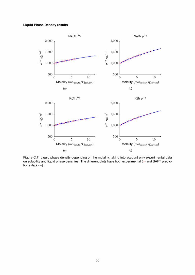
Liquid Phase Density results

0 5 10500

1,000

1,500

2,000

Molality (molsolute/kgsolvent)

ρliqkg/m

3

NaCl ρliq

(a)

0 5 10500

1,000

1,500

2,000

Molality (molsolute/kgsolvent)

ρliqkg/m

3

NaBr ρliq

(b)

0 5 10500

1,000

1,500

2,000

Molality (molsolute/kgsolvent)

ρliqkg/m

3

KCl ρliq

(c)

0 5 10500

1,000

1,500

2,000

Molality (molsolute/kgsolvent)

ρliqkg/m

3

KBr ρliq

(d)

Figure C.7: Liquid phase density depending on the molality, taking into account only experimental dataon solubility and liquid phase densities. The different plots have both experimental () and SAFT predic-tions data (−).

56

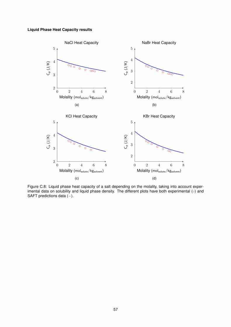
Liquid Phase Heat Capacity results

0 2 4 6 82

3

4

5

Molality (molsolute/kgsolvent)

Cp

(J/K

)NaCl Heat Capacity

(a)

0 2 4 6 8

2

3

4

5

Molality (molsolute/kgsolvent)

Cp

(J/K

)

NaBr Heat Capacity

(b)

0 2 4 6 82

3

4

5

Molality (molsolute/kgsolvent)

Cp

(J/K

)

KCl Heat Capacity

(c)

0 2 4 6 8

2

3

4

5

Molality (molsolute/kgsolvent)

Cp

(J/K

)

KBr Heat Capacity

(d)

Figure C.8: Liquid phase heat capacity of a salt depending on the molality, taking into account exper-imental data on solubility and liquid phase density. The different plots have both experimental () andSAFT predictions data (−).

57

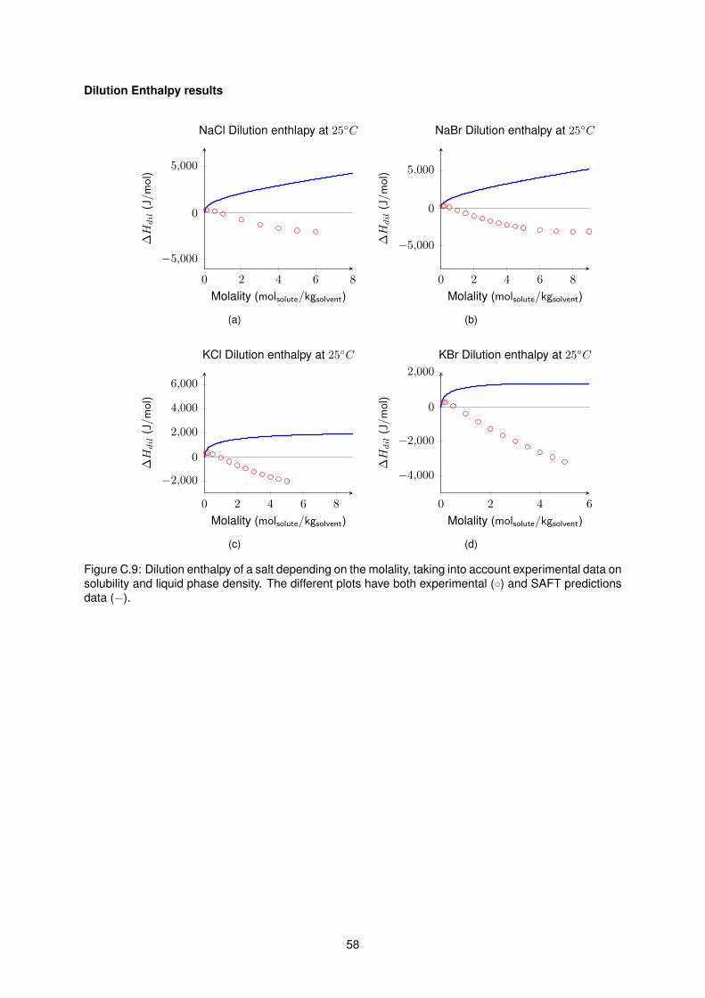
Dilution Enthalpy results

0 2 4 6 8

−5,000

0

5,000

Molality (molsolute/kgsolvent)

∆Hdil

(J/m

ol)

NaCl Dilution enthlapy at 25C

(a)

0 2 4 6 8

−5,000

0

5,000

Molality (molsolute/kgsolvent)

∆Hdil

(J/m

ol)

NaBr Dilution enthalpy at 25C

(b)

0 2 4 6 8

−2,000

0

2,000

4,000

6,000

Molality (molsolute/kgsolvent)

∆Hdil

(J/m

ol)

KCl Dilution enthalpy at 25C

(c)

0 2 4 6

−4,000

−2,000

0

2,000

Molality (molsolute/kgsolvent)

∆Hdil

(J/mol

)

KBr Dilution enthalpy at 25C

(d)

Figure C.9: Dilution enthalpy of a salt depending on the molality, taking into account experimental data onsolubility and liquid phase density. The different plots have both experimental () and SAFT predictionsdata (−).

58

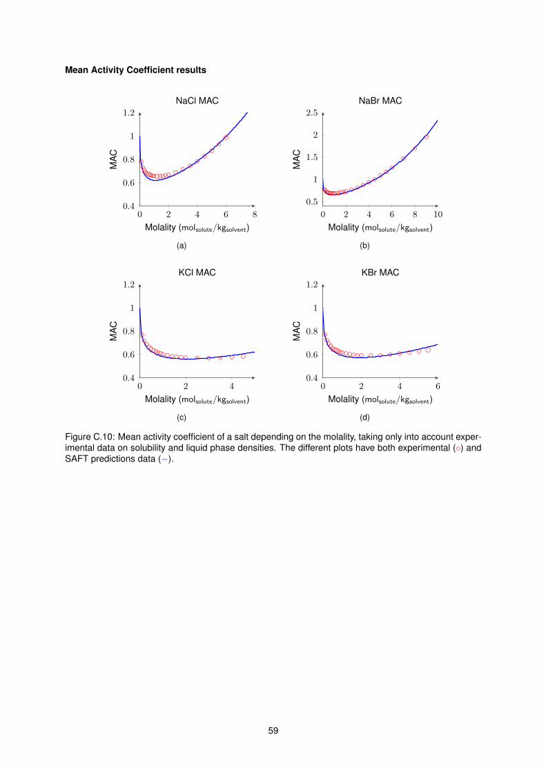
Mean Activity Coefficient results

0 2 4 6 80.4

0.6

0.8

1

1.2

Molality (molsolute/kgsolvent)

MA

CNaCl MAC

(a)

0 2 4 6 8 10

0.5

1

1.5

2

2.5

Molality (molsolute/kgsolvent)

MA

C

NaBr MAC

(b)

0 2 40.4

0.6

0.8

1

1.2

Molality (molsolute/kgsolvent)

MA

C

KCl MAC

(c)

0 2 4 60.4

0.6

0.8

1

1.2

Molality (molsolute/kgsolvent)

MA

C

KBr MAC

(d)

Figure C.10: Mean activity coefficient of a salt depending on the molality, taking only into account exper-imental data on solubility and liquid phase densities. The different plots have both experimental () andSAFT predictions data (−).

59

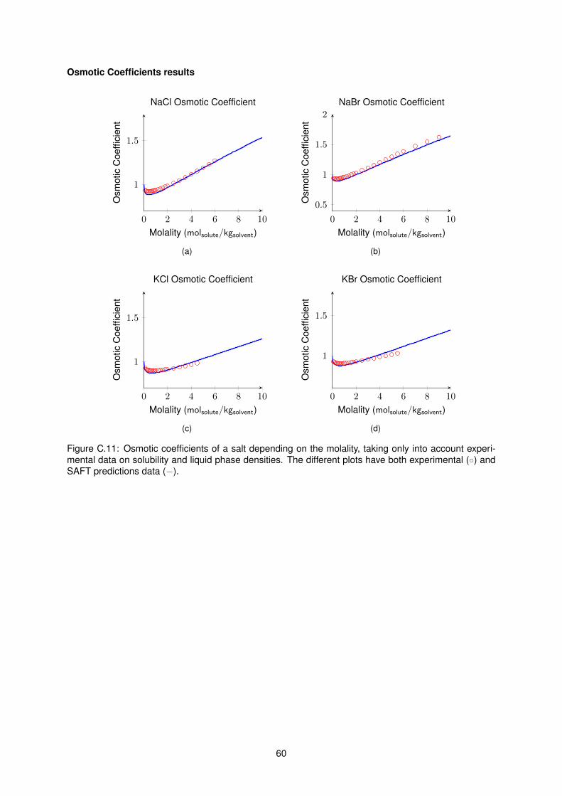
Osmotic Coefficients results

0 2 4 6 8 10

1

1.5

Molality (molsolute/kgsolvent)

Osm

otic

Coe

ffici

ent

NaCl Osmotic Coefficient

(a)

0 2 4 6 8 10

0.5

1

1.5

2

Molality (molsolute/kgsolvent)

Osm

otic

Coe

ffici

ent

NaBr Osmotic Coefficient

(b)

0 2 4 6 8 10

1

1.5

Molality (molsolute/kgsolvent)

Osm

otic

Coe

ffici

ent

KCl Osmotic Coefficient

(c)

0 2 4 6 8 10

1

1.5

Molality (molsolute/kgsolvent)

Osm

otic

Coe

ffici

ent

KBr Osmotic Coefficient

(d)

Figure C.11: Osmotic coefficients of a salt depending on the molality, taking only into account experi-mental data on solubility and liquid phase densities. The different plots have both experimental () andSAFT predictions data (−).

60

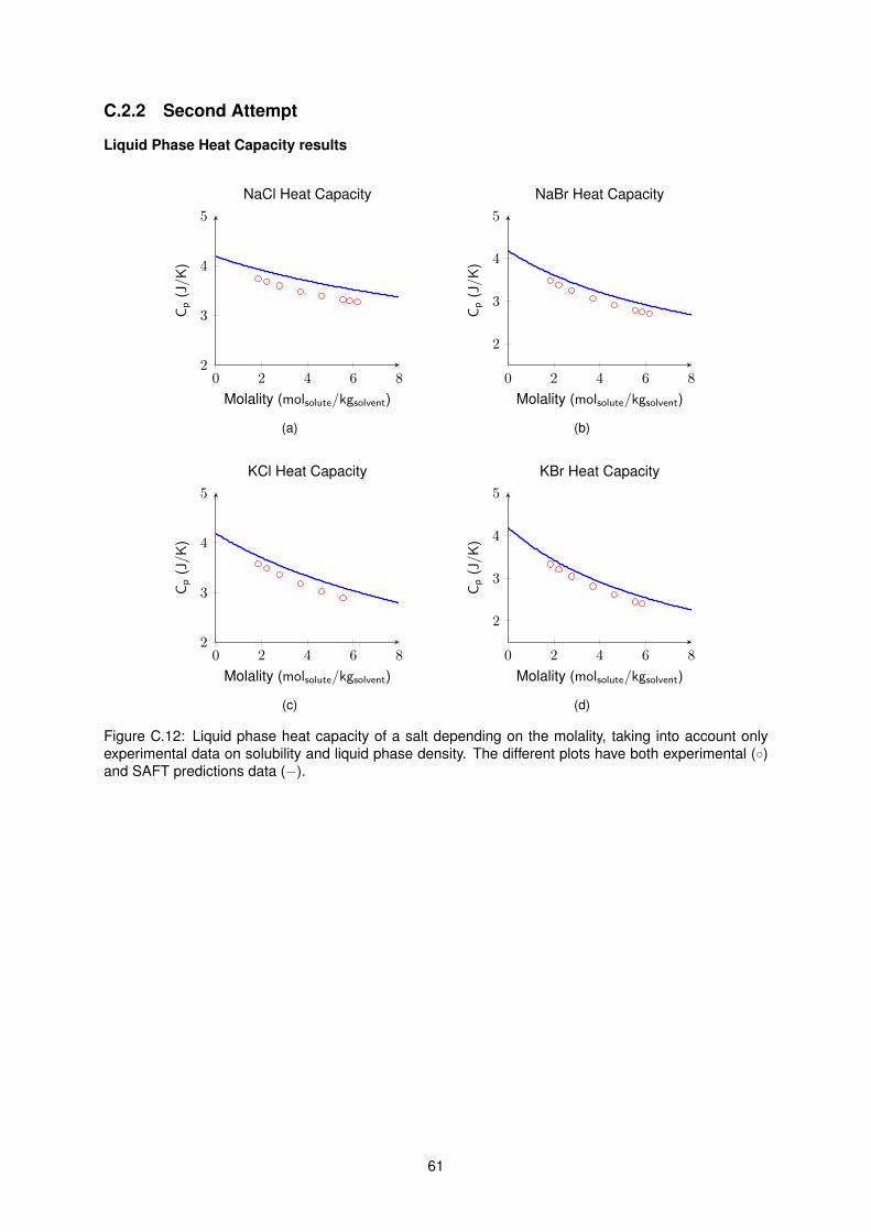
C.2.2 Second Attempt

Liquid Phase Heat Capacity results

0 2 4 6 82

3

4

5

Molality (molsolute/kgsolvent)

Cp

(J/K

)NaCl Heat Capacity

(a)

0 2 4 6 8

2

3

4

5

Molality (molsolute/kgsolvent)

Cp

(J/K

)

NaBr Heat Capacity

(b)

0 2 4 6 82

3

4

5

Molality (molsolute/kgsolvent)

Cp

(J/K

)

KCl Heat Capacity

(c)

0 2 4 6 8

2

3

4

5

Molality (molsolute/kgsolvent)

Cp

(J/K

)KBr Heat Capacity

(d)

Figure C.12: Liquid phase heat capacity of a salt depending on the molality, taking into account onlyexperimental data on solubility and liquid phase density. The different plots have both experimental ()and SAFT predictions data (−).

61

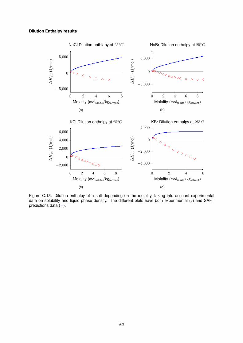
Dilution Enthalpy results

0 2 4 6 8

−5,000

0

5,000

Molality (molsolute/kgsolvent)

∆Hdil

(J/m

ol)

NaCl Dilution enthlapy at 25C

(a)

0 2 4 6 8

−5,000

0

5,000

Molality (molsolute/kgsolvent)

∆Hdil

(J/m

ol)

NaBr Dilution enthalpy at 25C

(b)

0 2 4 6 8

−2,000

0

2,000

4,000

6,000

Molality (molsolute/kgsolvent)

∆Hdil

(J/m

ol)

KCl Dilution enthalpy at 25C

(c)

0 2 4 6

−4,000

−2,000

0

2,000

Molality (molsolute/kgsolvent)

∆Hdil

(J/mol

)

KBr Dilution enthalpy at 25C

(d)

Figure C.13: Dilution enthalpy of a salt depending on the molality, taking into account experimentaldata on solubility and liquid phase density. The different plots have both experimental () and SAFTpredictions data (−).

62

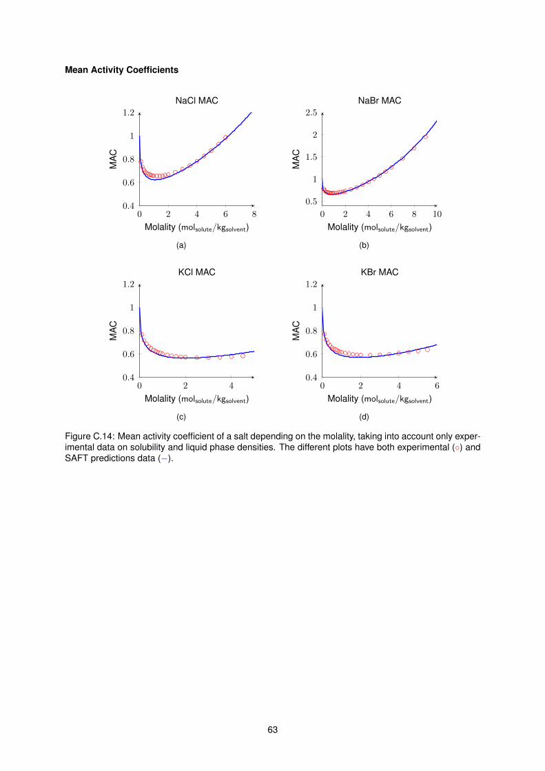
Mean Activity Coefficients

0 2 4 6 80.4

0.6

0.8

1

1.2

Molality (molsolute/kgsolvent)

MA

CNaCl MAC

(a)

0 2 4 6 8 10

0.5

1

1.5

2

2.5

Molality (molsolute/kgsolvent)

MA

C

NaBr MAC

(b)

0 2 40.4

0.6

0.8

1

1.2

Molality (molsolute/kgsolvent)

MA

C

KCl MAC

(c)

0 2 4 60.4

0.6

0.8

1

1.2

Molality (molsolute/kgsolvent)

MA

C

KBr MAC

(d)

Figure C.14: Mean activity coefficient of a salt depending on the molality, taking into account only exper-imental data on solubility and liquid phase densities. The different plots have both experimental () andSAFT predictions data (−).

63

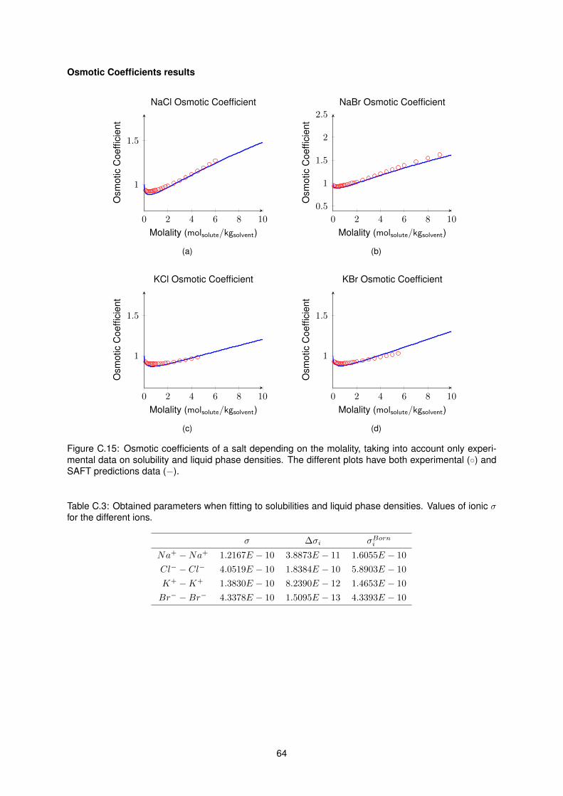
Osmotic Coefficients results

0 2 4 6 8 10

1

1.5

Molality (molsolute/kgsolvent)

Osm

otic

Coe

ffici

ent

NaCl Osmotic Coefficient

(a)

0 2 4 6 8 10

0.5

1

1.5

2

2.5

Molality (molsolute/kgsolvent)

Osm

otic

Coe

ffici

ent

NaBr Osmotic Coefficient

(b)

0 2 4 6 8 10

1

1.5

Molality (molsolute/kgsolvent)

Osm

otic

Coe

ffici

ent

KCl Osmotic Coefficient

(c)

0 2 4 6 8 10

1

1.5

Molality (molsolute/kgsolvent)

Osm

otic

Coe

ffici

ent

KBr Osmotic Coefficient

(d)

Figure C.15: Osmotic coefficients of a salt depending on the molality, taking into account only experi-mental data on solubility and liquid phase densities. The different plots have both experimental () andSAFT predictions data (−).

Table C.3: Obtained parameters when fitting to solubilities and liquid phase densities. Values of ionic σfor the different ions.

σ ∆σi σBorni

Na+ −Na+ 1.2167E − 10 3.8873E − 11 1.6055E − 10

Cl− − Cl− 4.0519E − 10 1.8384E − 10 5.8903E − 10

K+ −K+ 1.3830E − 10 8.2390E − 12 1.4653E − 10

Br− −Br− 4.3378E − 10 1.5095E − 13 4.3393E − 10

64

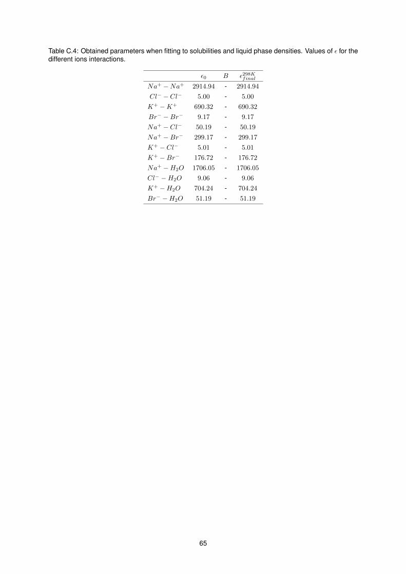
Table C.4: Obtained parameters when fitting to solubilities and liquid phase densities. Values of ε for thedifferent ions interactions.

ε0 B ε298Kfinal

Na+ −Na+ 2914.94 - 2914.94

Cl− − Cl− 5.00 - 5.00

K+ −K+ 690.32 - 690.32

Br− −Br− 9.17 - 9.17

Na+ − Cl− 50.19 - 50.19

Na+ −Br− 299.17 - 299.17

K+ − Cl− 5.01 - 5.01

K+ −Br− 176.72 - 176.72

Na+ −H2O 1706.05 - 1706.05

Cl− −H2O 9.06 - 9.06

K+ −H2O 704.24 - 704.24

Br− −H2O 51.19 - 51.19

65

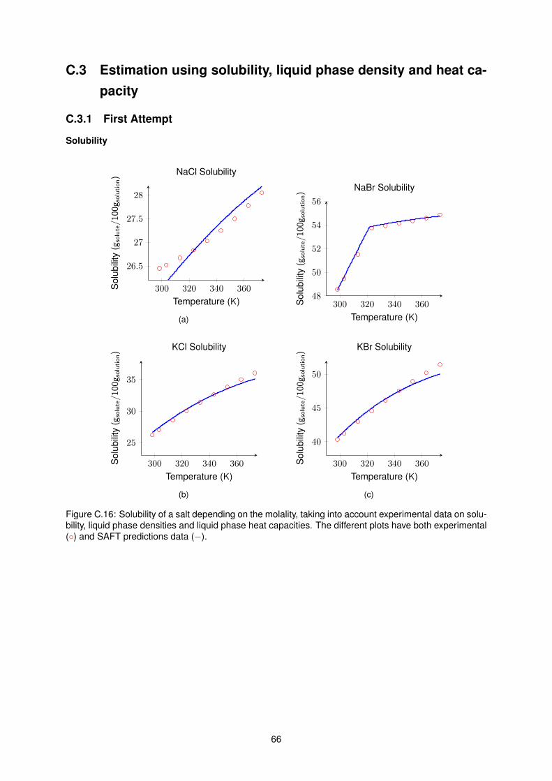
C.3 Estimation using solubility, liquid phase density and heat ca-pacity

C.3.1 First Attempt

Solubility

300 320 340 360

26.5

27

27.5

28

Temperature (K)

Sol

ubili

ty(g

solute/100g s

olution) NaCl Solubility

(a)

300 320 340 36048

50

52

54

56

Temperature (K)

Sol

ubili

ty(g

solute/100g s

olution) NaBr Solubility

300 320 340 360

25

30

35

Temperature (K)

Sol

ubili

ty(g

solute/100g s

olution) KCl Solubility

(b)

300 320 340 360

40

45

50

Temperature (K)

Sol

ubili

ty(g

solute/100g

solution) KBr Solubility

(c)

Figure C.16: Solubility of a salt depending on the molality, taking into account experimental data on solu-bility, liquid phase densities and liquid phase heat capacities. The different plots have both experimental() and SAFT predictions data (−).

66

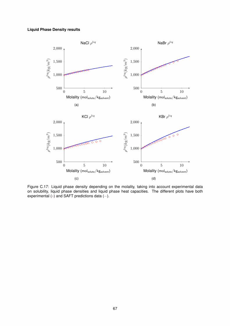
Liquid Phase Density results

0 5 10500

1,000

1,500

2,000

Molality (molsolute/kgsolvent)

ρliq(kg/m

3)

NaCl ρliq

(a)

0 5 10500

1,000

1,500

2,000

Molality (molsolute/kgsolvent)

ρliq(kg/m

3)

NaBr ρliq

(b)

0 5 10500

1,000

1,500

2,000

Molality (molsolute/kgsolvent)

ρliq(kg/m

3)

KCl ρliq

(c)

0 5 10500

1,000

1,500

2,000

Molality (molsolute/kgsolvent)

ρliq(kg/m

3)

KBr ρliq

(d)

Figure C.17: Liquid phase density depending on the molality, taking into account experimental dataon solubility, liquid phase densities and liquid phase heat capacities. The different plots have bothexperimental () and SAFT predictions data (−).

67

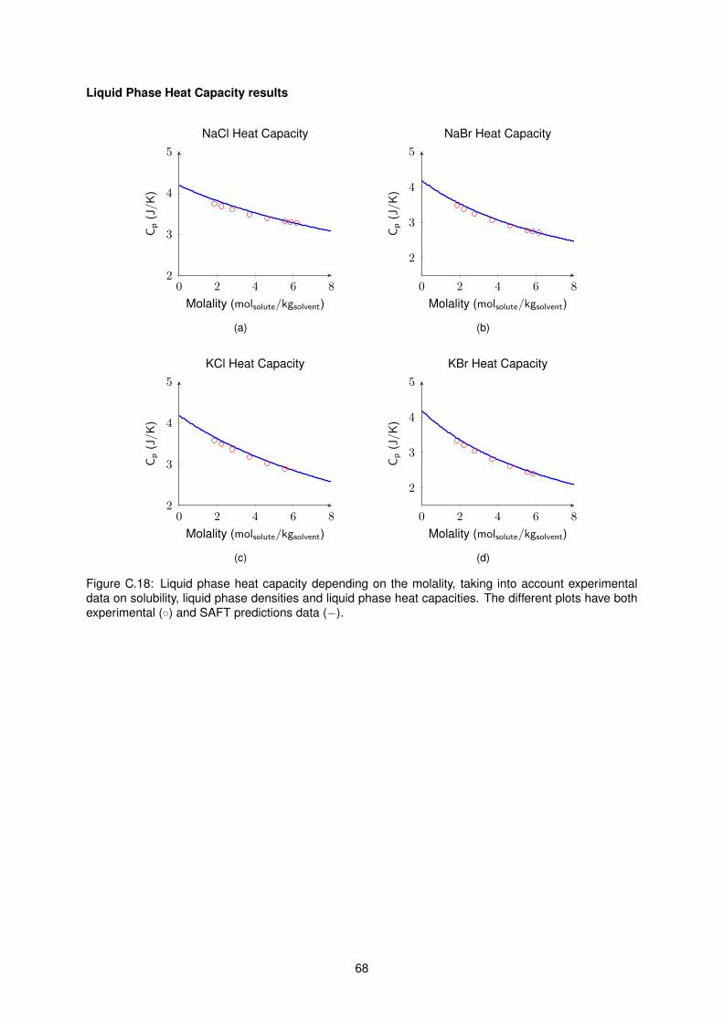
Liquid Phase Heat Capacity results

0 2 4 6 82

3

4

5

Molality (molsolute/kgsolvent)

Cp

(J/K

)NaCl Heat Capacity

(a)

0 2 4 6 8

2

3

4

5

Molality (molsolute/kgsolvent)

Cp

(J/K

)

NaBr Heat Capacity

(b)

0 2 4 6 82

3

4

5

Molality (molsolute/kgsolvent)

Cp

(J/K

)

KCl Heat Capacity

(c)

0 2 4 6 8

2

3

4

5

Molality (molsolute/kgsolvent)

Cp

(J/K

)

KBr Heat Capacity

(d)

Figure C.18: Liquid phase heat capacity depending on the molality, taking into account experimentaldata on solubility, liquid phase densities and liquid phase heat capacities. The different plots have bothexperimental () and SAFT predictions data (−).

68

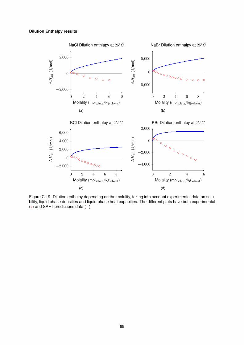
Dilution Enthalpy results

0 2 4 6 8

−5,000

0

5,000

Molality (molsolute/kgsolvent)

∆Hdil

(J/m

ol)

NaCl Dilution enthlapy at 25C

(a)

0 2 4 6 8

−5,000

0

5,000

Molality (molsolute/kgsolvent)

∆Hdil

(J/m

ol)

NaBr Dilution enthalpy at 25C

(b)

0 2 4 6 8

−2,000

0

2,000

4,000

6,000

Molality (molsolute/kgsolvent)

∆Hdil

(J/m

ol)

KCl Dilution enthalpy at 25C

(c)

0 2 4 6

−4,000

−2,000

0

2,000

Molality (molsolute/kgsolvent)

∆Hdil

(J/mol

)

KBr Dilution enthalpy at 25C

(d)

Figure C.19: Dilution enthalpy depending on the molality, taking into account experimental data on solu-bility, liquid phase densities and liquid phase heat capacities. The different plots have both experimental() and SAFT predictions data (−).

69

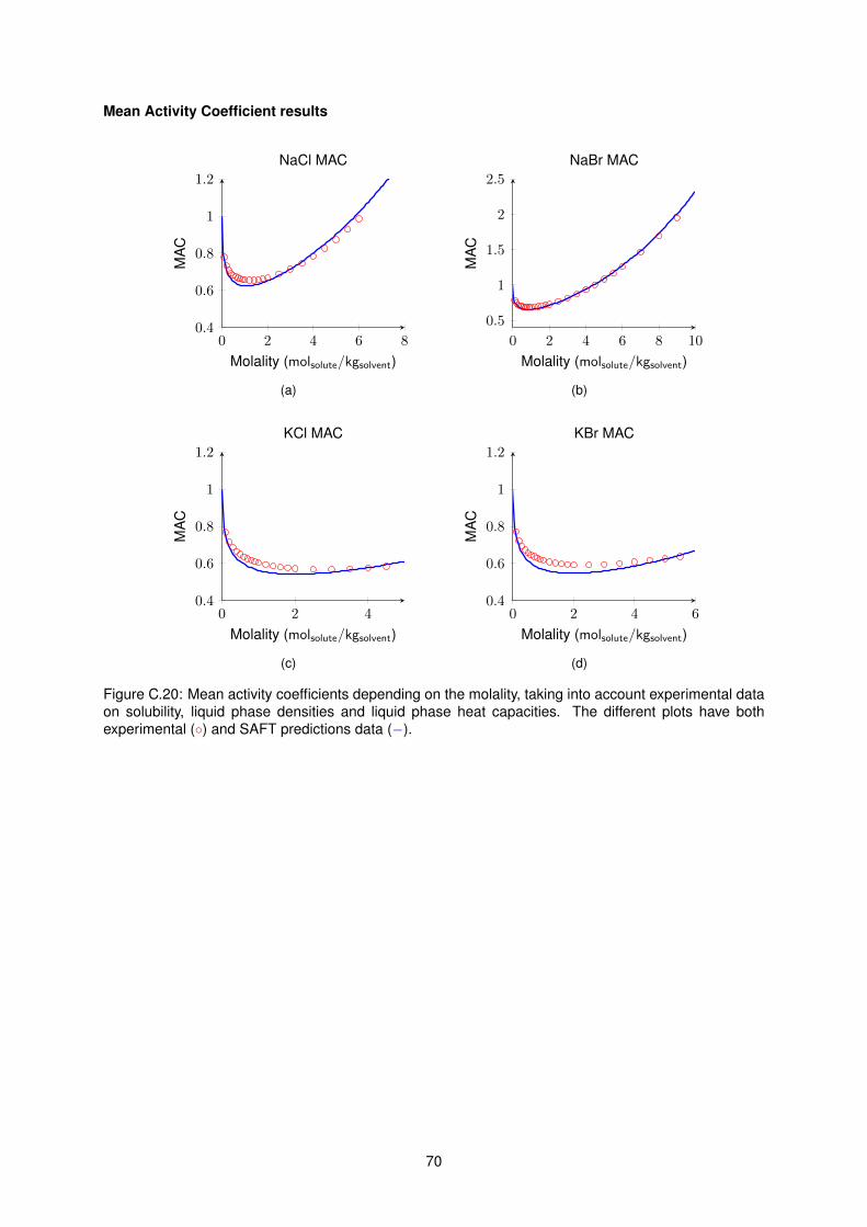
Mean Activity Coefficient results

0 2 4 6 80.4

0.6

0.8

1

1.2

Molality (molsolute/kgsolvent)

MA

CNaCl MAC

(a)

0 2 4 6 8 10

0.5

1

1.5

2

2.5

Molality (molsolute/kgsolvent)

MA

C

NaBr MAC

(b)

0 2 40.4

0.6

0.8

1

1.2

Molality (molsolute/kgsolvent)

MA

C

KCl MAC

(c)

0 2 4 60.4

0.6

0.8

1

1.2

Molality (molsolute/kgsolvent)

MA

C

KBr MAC

(d)

Figure C.20: Mean activity coefficients depending on the molality, taking into account experimental dataon solubility, liquid phase densities and liquid phase heat capacities. The different plots have bothexperimental () and SAFT predictions data (−).

70

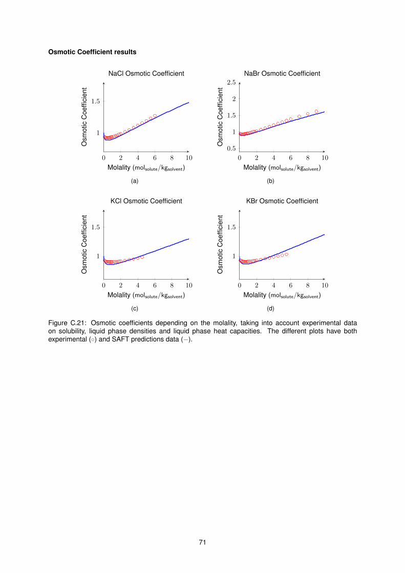
Osmotic Coefficient results

0 2 4 6 8 10

1

1.5

Molality (molsolute/kgsolvent)

Osm

otic

Coe

ffici

ent

NaCl Osmotic Coefficient

(a)

0 2 4 6 8 10

0.5

1

1.5

2

2.5

Molality (molsolute/kgsolvent)

Osm

otic

Coe

ffici

ent

NaBr Osmotic Coefficient

(b)

0 2 4 6 8 10

1

1.5

Molality (molsolute/kgsolvent)

Osm

otic

Coe

ffici

ent

KCl Osmotic Coefficient

(c)

0 2 4 6 8 10

1

1.5

Molality (molsolute/kgsolvent)

Osm

otic

Coe

ffici

ent

KBr Osmotic Coefficient

(d)

Figure C.21: Osmotic coefficients depending on the molality, taking into account experimental dataon solubility, liquid phase densities and liquid phase heat capacities. The different plots have bothexperimental () and SAFT predictions data (−).

71

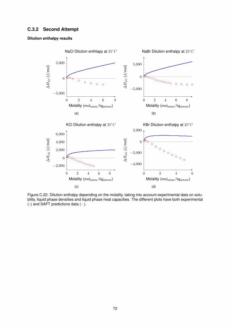
C.3.2 Second Attempt

Dilution enthalpy results

0 2 4 6 8

−5,000

0

5,000

Molality (molsolute/kgsolvent)

∆Hdil

(J/m

ol)

NaCl Dilution enthlapy at 25C

(a)

0 2 4 6 8

−5,000

0

5,000

Molality (molsolute/kgsolvent)

∆Hdil

(J/m

ol)

NaBr Dilution enthalpy at 25C

(b)

0 2 4 6 8

−2,000

0

2,000

4,000

6,000

Molality (molsolute/kgsolvent)

∆Hdil

(J/m

ol)

KCl Dilution enthalpy at 25C

(c)

0 2 4 6

−4,000

−2,000

0

2,000

Molality (molsolute/kgsolvent)

∆Hdil

(J/mol

)KBr Dilution enthalpy at 25C

(d)

Figure C.22: Dilution enthalpy depending on the molality, taking into account experimental data on solu-bility, liquid phase densities and liquid phase heat capacities. The different plots have both experimental() and SAFT predictions data (−).

72

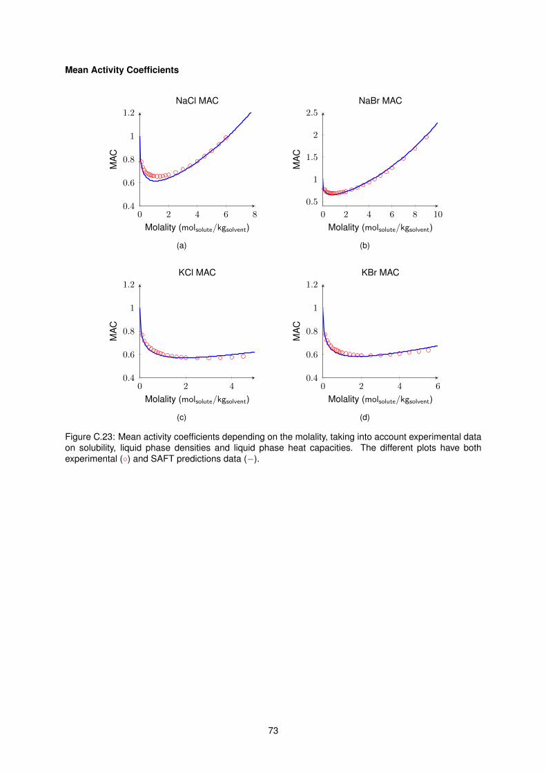
Mean Activity Coefficients

0 2 4 6 80.4

0.6

0.8

1

1.2

Molality (molsolute/kgsolvent)

MA

CNaCl MAC

(a)

0 2 4 6 8 10

0.5

1

1.5

2

2.5

Molality (molsolute/kgsolvent)

MA

C

NaBr MAC

(b)

0 2 40.4

0.6

0.8

1

1.2

Molality (molsolute/kgsolvent)

MA

C

KCl MAC

(c)

0 2 4 60.4

0.6

0.8

1

1.2

Molality (molsolute/kgsolvent)

MA

C

KBr MAC

(d)

Figure C.23: Mean activity coefficients depending on the molality, taking into account experimental dataon solubility, liquid phase densities and liquid phase heat capacities. The different plots have bothexperimental () and SAFT predictions data (−).

73

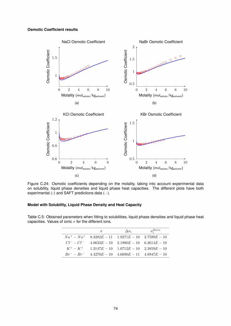
Osmotic Coefficient results

0 2 4 6 8 10

1

1.5

Molality (molsolute/kgsolvent)

Osm

otic

Coe

ffici

ent

NaCl Osmotic Coefficient

(a)

0 2 4 6 8 10

0.5

1

1.5

2

Molality (molsolute/kgsolvent)

Osm

otic

Coe

ffici

ent

NaBr Osmotic Coefficient

(b)

0 2 4 6 80.6

0.8

1

1.2

Molality (molsolute/kgsolvent)

Osm

otic

Coe

ffici

ent

KCl Osmotic Coefficient

(c)

0 2 4 6 8 100.5

1

1.5

Molality (molsolute/kgsolvent)

Osm

otic

Coe

ffici

ent

KBr Osmotic Coefficient

(d)

Figure C.24: Osmotic coefficients depending on the molality, taking into account experimental dataon solubility, liquid phase densities and liquid phase heat capacities. The different plots have bothexperimental () and SAFT predictions data (−).

Model with Solubility, Liquid Phase Density and Heat Capacity

Table C.5: Obtained parameters when fitting to solubilities, liquid phase densities and liquid phase heatcapacities. Values of ionic σ for the different ions.

σ ∆σi σBorni

Na+ −Na+ 8.3282E − 11 1.9271E − 10 2.7599E − 10

Cl− − Cl− 4.0633E − 10 2.1980E − 10 6.2614E − 10

K+ −K+ 1.3147E − 10 1.0712E − 10 2.3859E − 10

Br− −Br− 4.4278E − 10 4.6690E − 11 4.8947E − 10

74

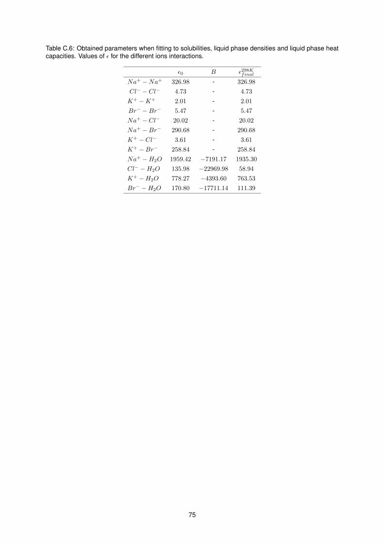
Table C.6: Obtained parameters when fitting to solubilities, liquid phase densities and liquid phase heatcapacities. Values of ε for the different ions interactions.

ε0 B ε298Kfinal

Na+ −Na+ 326.98 - 326.98

Cl− − Cl− 4.73 - 4.73

K+ −K+ 2.01 - 2.01

Br− −Br− 5.47 - 5.47

Na+ − Cl− 20.02 - 20.02

Na+ −Br− 290.68 - 290.68

K+ − Cl− 3.61 - 3.61

K+ −Br− 258.84 - 258.84

Na+ −H2O 1959.42 −7191.17 1935.30

Cl− −H2O 135.98 −22969.98 58.94

K+ −H2O 778.27 −4393.60 763.53

Br− −H2O 170.80 −17711.14 111.39

75

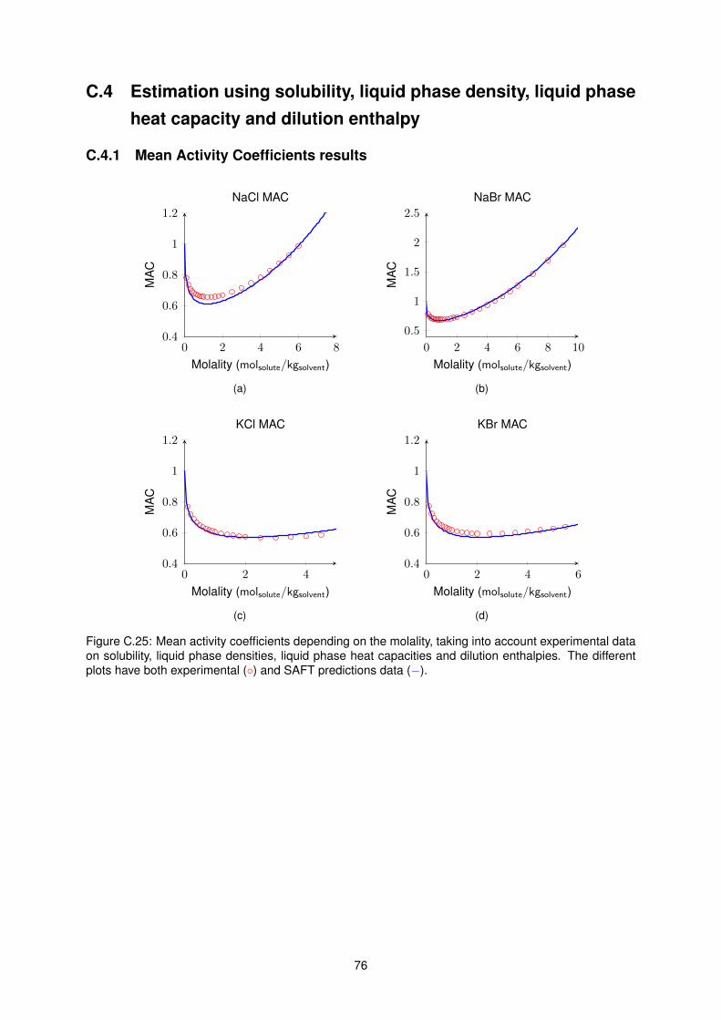
C.4 Estimation using solubility, liquid phase density, liquid phaseheat capacity and dilution enthalpy

C.4.1 Mean Activity Coefficients results

0 2 4 6 80.4

0.6

0.8

1

1.2

Molality (molsolute/kgsolvent)

MA

C

NaCl MAC

(a)

0 2 4 6 8 10

0.5

1

1.5

2

2.5

Molality (molsolute/kgsolvent)

MA

C

NaBr MAC

(b)

0 2 40.4

0.6

0.8

1

1.2

Molality (molsolute/kgsolvent)

MA

C

KCl MAC

(c)

0 2 4 60.4

0.6

0.8

1

1.2

Molality (molsolute/kgsolvent)

MA

C

KBr MAC

(d)

Figure C.25: Mean activity coefficients depending on the molality, taking into account experimental dataon solubility, liquid phase densities, liquid phase heat capacities and dilution enthalpies. The differentplots have both experimental () and SAFT predictions data (−).

76

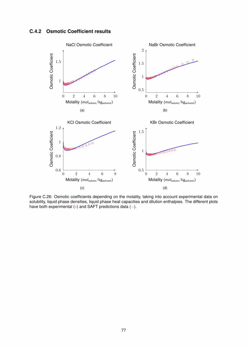
C.4.2 Osmotic Coefficient results

0 2 4 6 8 10

1

1.5

Molality (molsolute/kgsolvent)

Osm

otic

Coe

ffici

ent

NaCl Osmotic Coefficient

(a)

0 2 4 6 8 10

0.5

1

1.5

2

Molality (molsolute/kgsolvent)

Osm

otic

Coe

ffici

ent

NaBr Osmotic Coefficient

(b)

0 2 4 6 80.6

0.8

1

1.2

Molality (molsolute/kgsolvent)

Osm

otic

Coe

ffici

ent

KCl Osmotic Coefficient

(c)

0 2 4 6 8 100.5

1

1.5

Molality (molsolute/kgsolvent)

Osm

otic

Coe

ffici

ent

KBr Osmotic Coefficient

(d)

Figure C.26: Osmotic coefficients depending on the molality, taking into account experimental data onsolubility, liquid phase densities, liquid phase heat capacities and dilution enthalpies. The different plotshave both experimental () and SAFT predictions data (−).

77

C.5 Model Extension

C.5.1 Mean Activity Coefficients results

0 5 100

0.5

1

Molality (molsolute/kgsolvent)

MA

C

RbCl

RbBr

0 5 100

0.5

1

Molality (molsolute/kgsolvent)

MA

C

CsCl

CsBr

0 5 100

0.5

1

Molality (molsolute/kgsolvent)

MA

C

NH4Cl

NH4Br

0 5 100.5

1

1.5

2

Molality (molsolute/kgsolvent)

MA

C

NaI

KI

0 5 100

0.5

1

Molality (molsolute/kgsolvent)

MA

C

NaNO3KNO3

Figure C.27: Mean activity coefficients for the final model extension

78

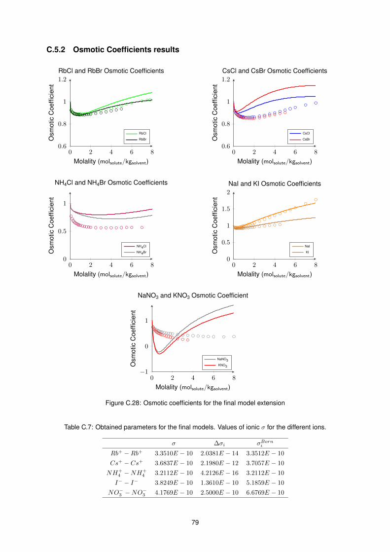
C.5.2 Osmotic Coefficients results

0 2 4 6 80.6

0.8

1

1.2

Molality (molsolute/kgsolvent)

Osm

otic

Coe

ffici

ent

RbCl and RbBr Osmotic Coefficients

RbCl

RbBr

0 2 4 6 80.6

0.8

1

1.2

Molality (molsolute/kgsolvent)

Osm

otic

Coe

ffici

ent

CsCl and CsBr Osmotic Coefficients

CsCl

CsBr

0 2 4 6 80

0.5

1

Molality (molsolute/kgsolvent)

Osm

otic

Coe

ffici

ent

NH4Cl and NH4Br Osmotic Coefficients

NH4Cl

NH4Br

0 2 4 6 80

0.5

1

1.5

2

Molality (molsolute/kgsolvent)

Osm

otic

Coe

ffici

ent

NaI and KI Osmotic Coefficients

NaI

KI

0 2 4 6 8−1

0

1

Molality (molsolute/kgsolvent)

Osm

otic

Coe

ffici

ent

NaNO3 and KNO3 Osmotic Coefficient

NaNO3KNO3

Figure C.28: Osmotic coefficients for the final model extension

Table C.7: Obtained parameters for the final models. Values of ionic σ for the different ions.

σ ∆σi σBorni

Rb+ −Rb+ 3.3510E − 10 2.0381E − 14 3.3512E − 10

Cs+ − Cs+ 3.6837E − 10 2.1980E − 12 3.7057E − 10

NH+4 −NH

+4 3.2112E − 10 4.2126E − 16 3.2112E − 10

I− − I− 3.8249E − 10 1.3610E − 10 5.1859E − 10

NO−3 −NO−3 4.1769E − 10 2.5000E − 10 6.6769E − 10

79

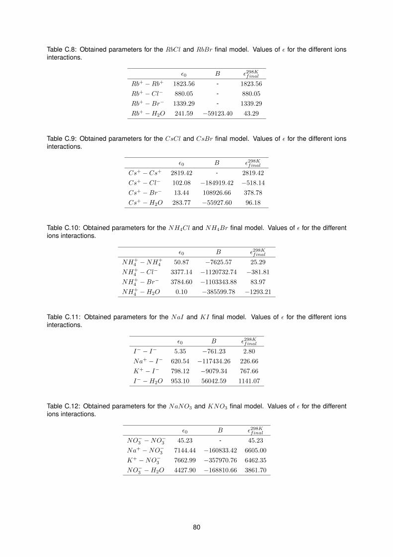
Table C.8: Obtained parameters for the RbCl and RbBr final model. Values of ε for the different ionsinteractions.

ε0 B ε298Kfinal

Rb+ −Rb+ 1823.56 - 1823.56

Rb+ − Cl− 880.05 - 880.05

Rb+ −Br− 1339.29 - 1339.29

Rb+ −H2O 241.59 −59123.40 43.29

Table C.9: Obtained parameters for the CsCl and CsBr final model. Values of ε for the different ionsinteractions.

ε0 B ε298Kfinal

Cs+ − Cs+ 2819.42 - 2819.42

Cs+ − Cl− 102.08 −184919.42 −518.14

Cs+ −Br− 13.44 108926.66 378.78

Cs+ −H2O 283.77 −55927.60 96.18

Table C.10: Obtained parameters for the NH4Cl and NH4Br final model. Values of ε for the differentions interactions.

ε0 B ε298Kfinal

NH+4 −NH

+4 50.87 −7625.57 25.29

NH+4 − Cl− 3377.14 −1120732.74 −381.81

NH+4 −Br− 3784.60 −1103343.88 83.97

NH+4 −H2O 0.10 −385599.78 −1293.21

Table C.11: Obtained parameters for the NaI and KI final model. Values of ε for the different ionsinteractions.

ε0 B ε298Kfinal

I− − I− 5.35 −761.23 2.80

Na+ − I− 620.54 −117434.26 226.66

K+ − I− 798.12 −9079.34 767.66

I− −H2O 953.10 56042.59 1141.07

Table C.12: Obtained parameters for the NaNO3 and KNO3 final model. Values of ε for the differentions interactions.

ε0 B ε298Kfinal

NO−3 −NO−3 45.23 - 45.23

Na+ −NO−3 7144.44 −160833.42 6605.00

K+ −NO−3 7662.99 −357970.76 6462.35

NO−3 −H2O 4427.90 −168810.66 3861.70

80