


γλώσσες
Σελίδες
Νομικός


HW4 has been posted.
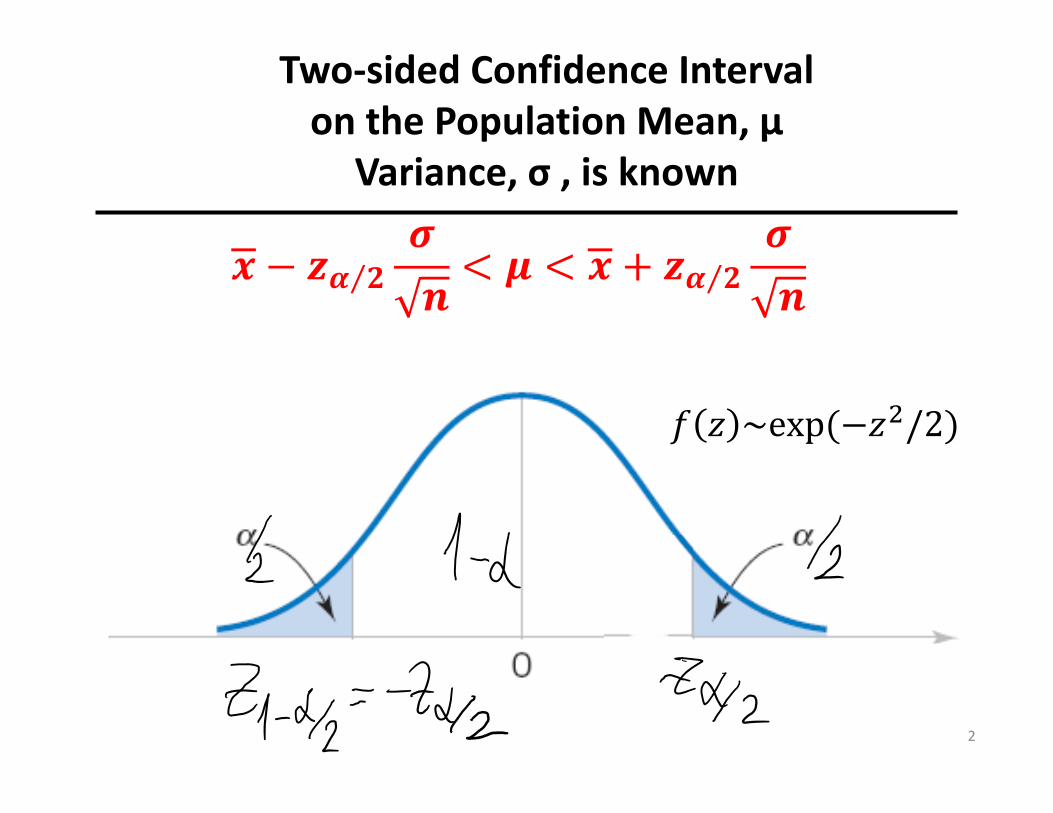
𝜶 𝟐⁄ 𝜶 𝟐⁄
Two‐sided Confidence Interval on the Population Mean, µ
Variance, σ , is known
2
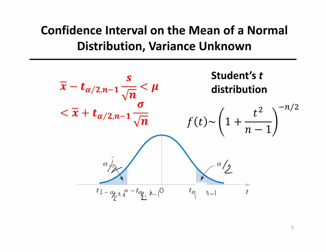
Student’s tdistribution
Confidence Interval on the Mean of a Normal Distribution, Variance Unknown
3
/
𝜶 𝟐,𝒏 𝟏⁄
𝜶 𝟐,𝒏 𝟏⁄
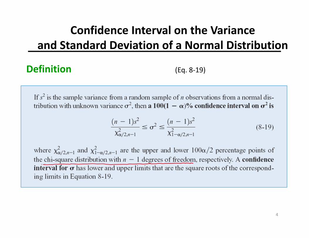
Definition (Eq. 8‐19)
Confidence Interval on the Variance and Standard Deviation of a Normal Distribution
4
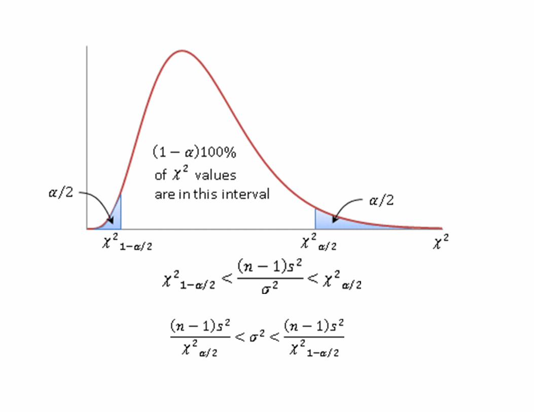
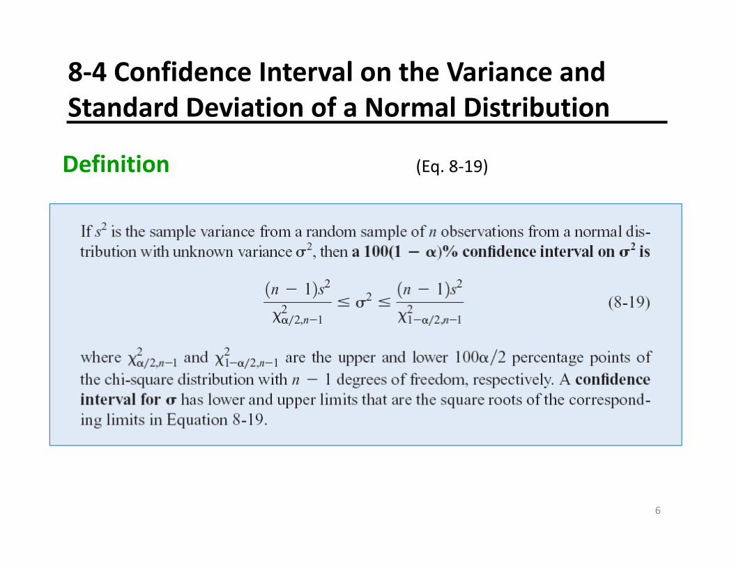
Definition (Eq. 8‐19)
8‐4 Confidence Interval on the Variance and Standard Deviation of a Normal Distribution
6
Confidence estimates of the population proportion
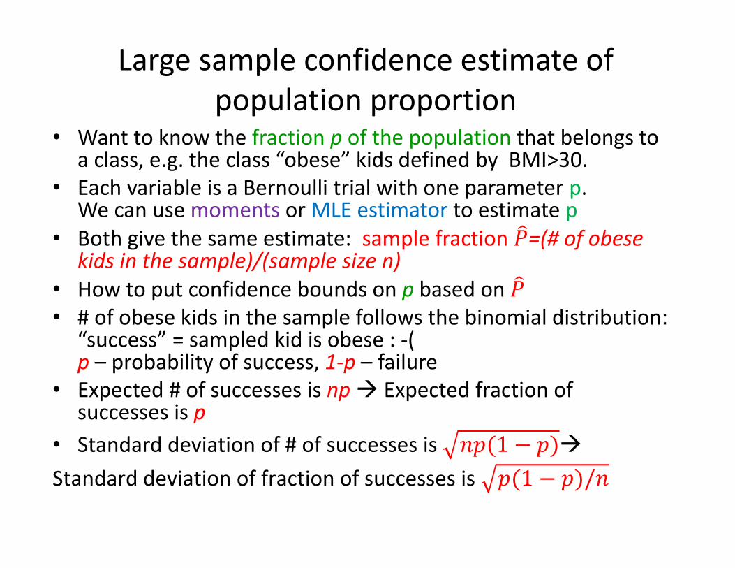
Large sample confidence estimate of population proportion
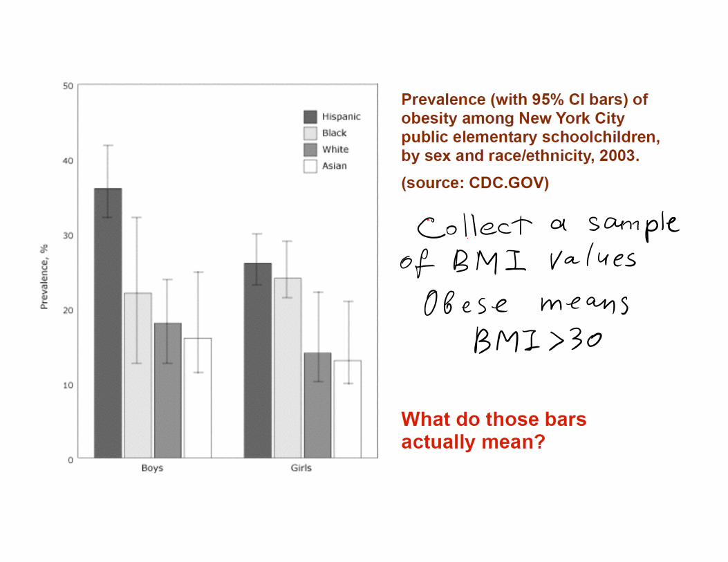
• Want to know the fraction p of the population that belongs to a class, e.g. the class “obese” kids defined by BMI>30.
• Each variable is a Bernoulli trial with one parameter p. We can use moments or MLE estimator to estimate p
• Both give the same estimate: sample fraction 𝑃=(# of obese kids in the sample)/(sample size n)
• How to put confidence bounds on p based on 𝑃• # of obese kids in the sample follows the binomial distribution:
“success” = sampled kid is obese : ‐(p – probability of success, 1‐p – failure
• Expected # of successes is np Expected fraction of successes is p
• Standard deviation of # of successes is 𝑛𝑝 1 𝑝 Standard deviation of fraction of successes is 𝑝 1 𝑝 /𝑛
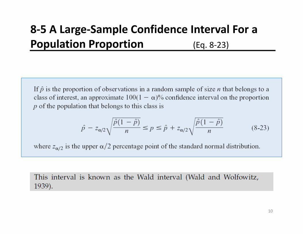
8‐5 A Large‐Sample Confidence Interval For a Population Proportion (Eq. 8‐23)
10
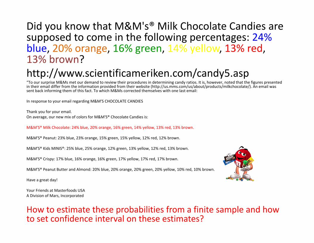
Did you know that M&M's® Milk Chocolate Candies are supposed to come in the following percentages: 24% blue, 20% orange, 16% green, 14% yellow, 13% red, 13% brown? http://www.scientificameriken.com/candy5.asp“To our surprise M&Ms met our demand to review their procedures in determining candy ratios. It is, however, noted that the figures presented in their email differ from the information provided from their website (http://us.mms.com/us/about/products/milkchocolate/). An email was sent back informing them of this fact. To which M&Ms corrected themselves with one last email:
In response to your email regarding M&M'S CHOCOLATE CANDIES
Thank you for your email.On average, our new mix of colors for M&M'S® Chocolate Candies is:
M&M'S® Milk Chocolate: 24% blue, 20% orange, 16% green, 14% yellow, 13% red, 13% brown.
M&M'S® Peanut: 23% blue, 23% orange, 15% green, 15% yellow, 12% red, 12% brown.
M&M'S® Kids MINIS®: 25% blue, 25% orange, 12% green, 13% yellow, 12% red, 13% brown.
M&M'S® Crispy: 17% blue, 16% orange, 16% green, 17% yellow, 17% red, 17% brown.
M&M'S® Peanut Butter and Almond: 20% blue, 20% orange, 20% green, 20% yellow, 10% red, 10% brown.
Have a great day!
Your Friends at Masterfoods USAA Division of Mars, Incorporated
How to estimate these probabilities from a finite sample and how to set confidence interval on these estimates?
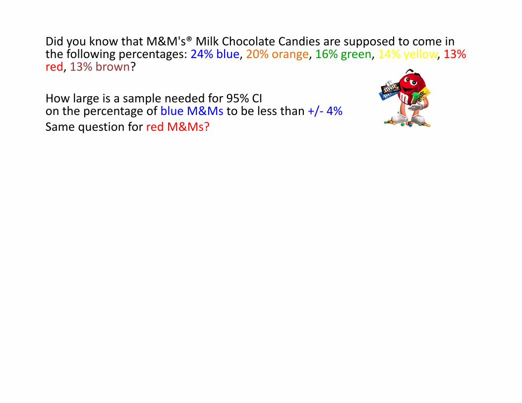
Did you know that M&M's® Milk Chocolate Candies are supposed to come in the following percentages: 24% blue, 20% orange, 16% green, 14% yellow, 13% red, 13% brown?
How large is a sample needed for 95% CI on the percentage of blue M&Ms to be less than +/‐ 4%Same question for red M&Ms?
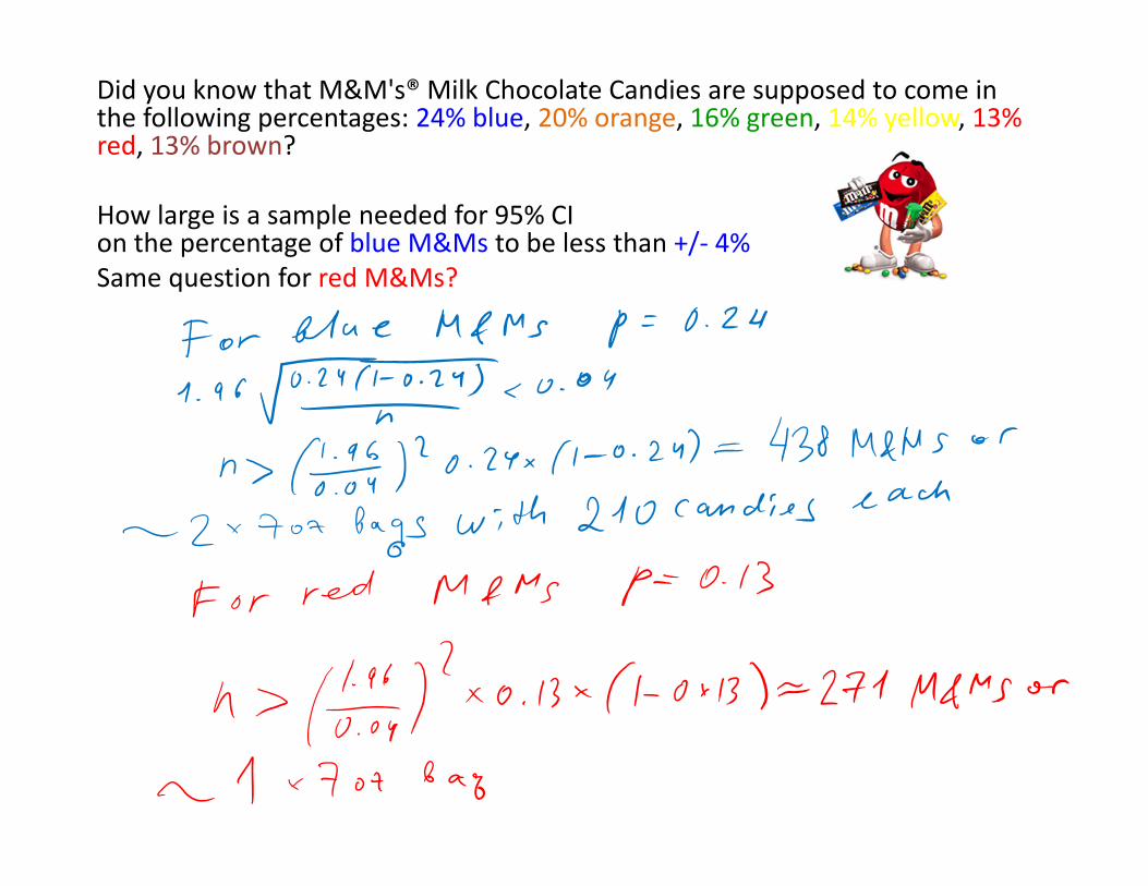
Did you know that M&M's® Milk Chocolate Candies are supposed to come in the following percentages: 24% blue, 20% orange, 16% green, 14% yellow, 13% red, 13% brown?
How large is a sample needed for 95% CI on the percentage of blue M&Ms to be less than +/‐ 4%Same question for red M&Ms?
Hypothesis testing:one sample
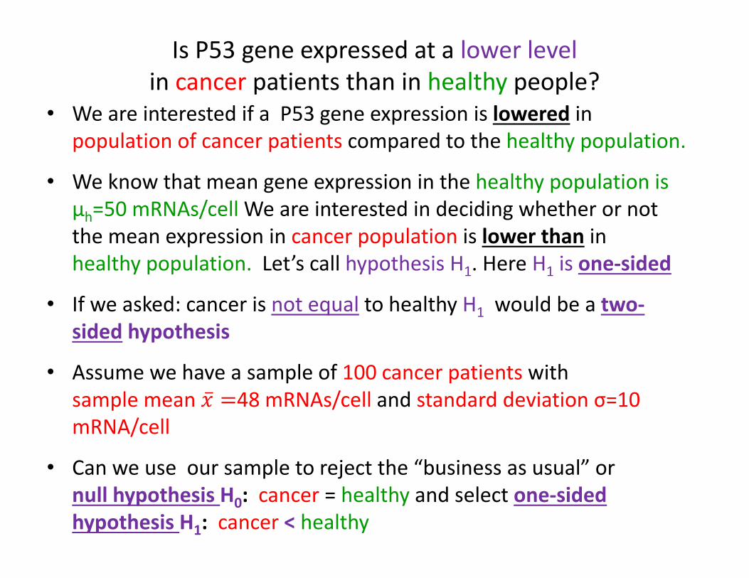
• We are interested if a P53 gene expression is lowered in population of cancer patients compared to the healthy population.
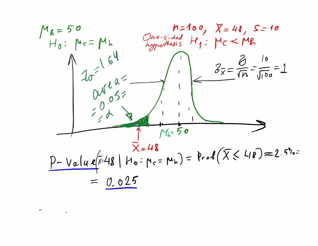
• We know that mean gene expression in the healthy population is μh=50 mRNAs/cell We are interested in deciding whether or notthe mean expression in cancer population is lower than in healthy population. Let’s call hypothesis H1. Here H1 is one‐sided
• If we asked: cancer is not equal to healthy H1 would be a two‐sided hypothesis
• Assume we have a sample of 100 cancer patients with sample mean 𝑥 48 mRNAs/cell and standard deviation σ=10 mRNA/cell
• Can we use our sample to reject the “business as usual” or null hypothesis H0: cancer = healthy and select one‐sided hypothesis H1: cancer < healthy
Is P53 gene expressed at a lower levelin cancer patients than in healthy people?
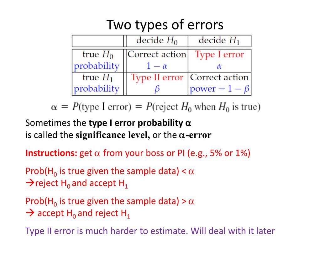
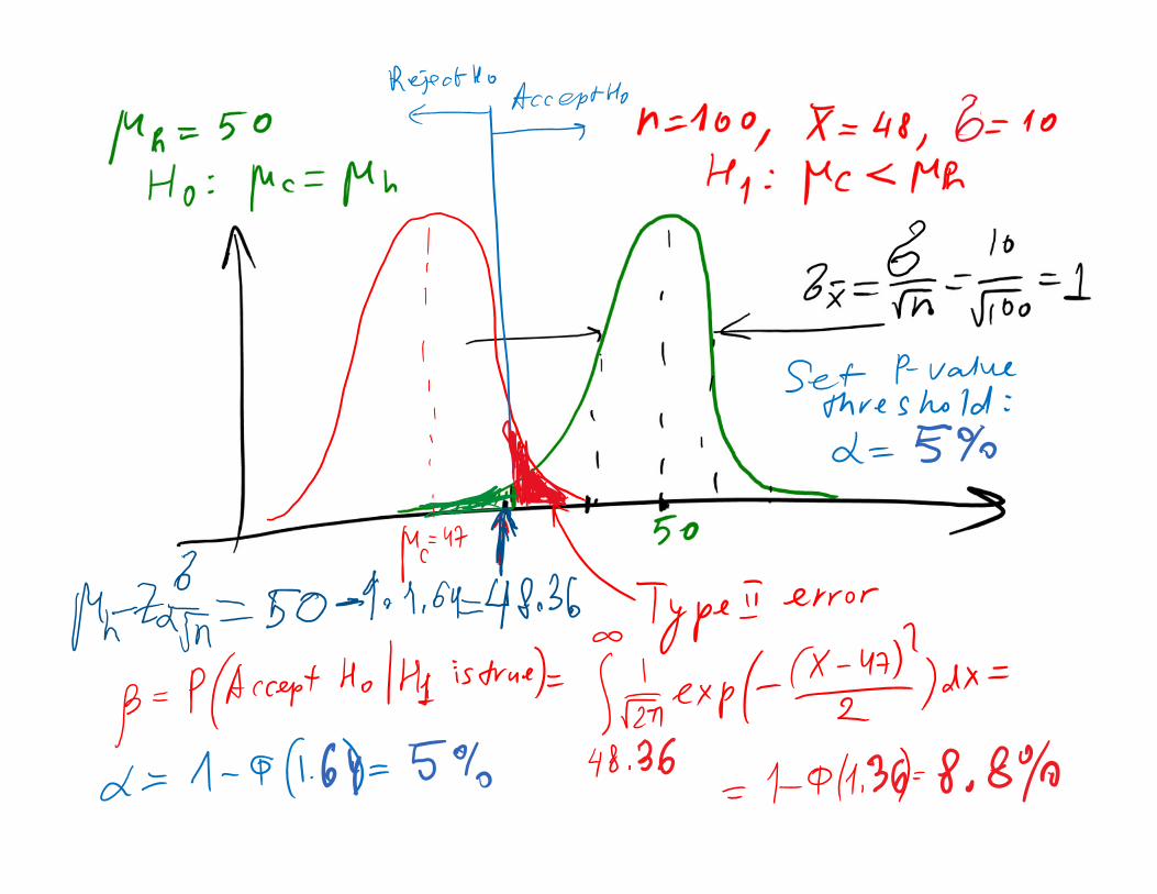
Two types of errors
Sometimes the type I error probability αis called the significance level, or the -error
Instructions: get from your boss or PI (e.g., 5% or 1%)
Prob(H0 is true given the sample data) < reject H0 and accept H1
Prob(H0 is true given the sample data) > accept H0 and reject H1
Type II error is much harder to estimate. Will deal with it later
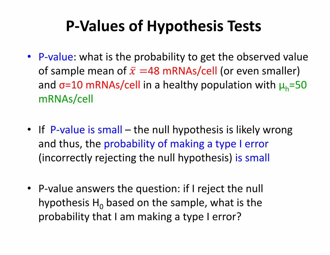
P‐Values of Hypothesis Tests
• P‐value: what is the probability to get the observed value of sample mean of 48 mRNAs/cell (or even smaller) and σ=10 mRNAs/cell in a healthy population with μh=50 mRNAs/cell
• If P‐value is small – the null hypothesis is likely wrong and thus, the probability of making a type I error (incorrectly rejecting the null hypothesis) is small
• P‐value answers the question: if I reject the null hypothesis H0 based on the sample, what is the probability that I am making a type I error?
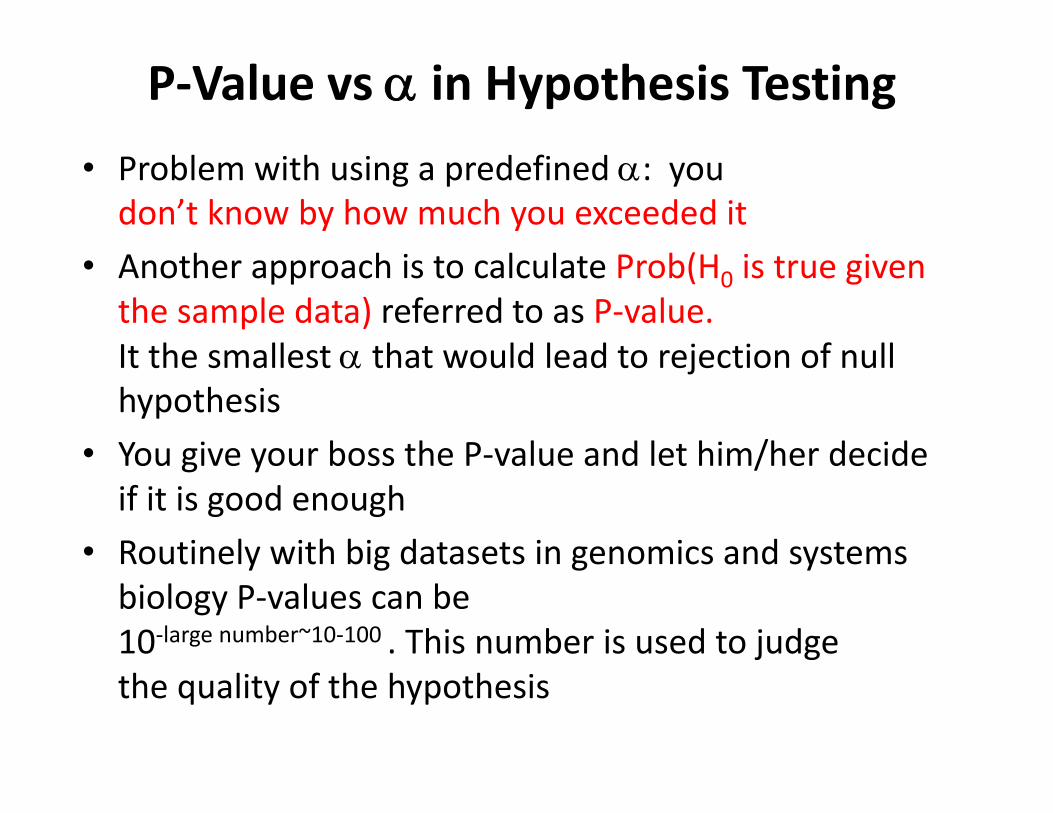
P‐Value vs in Hypothesis Testing• Problem with using a predefined : you don’t know by how much you exceeded it
• Another approach is to calculate Prob(H0 is true given the sample data) referred to as P‐value. It the smallest that would lead to rejection of null hypothesis
• You give your boss the P‐value and let him/her decide if it is good enough
• Routinely with big datasets in genomics and systems biology P‐values can be 10‐large number~10‐100 . This number is used to judge the quality of the hypothesis


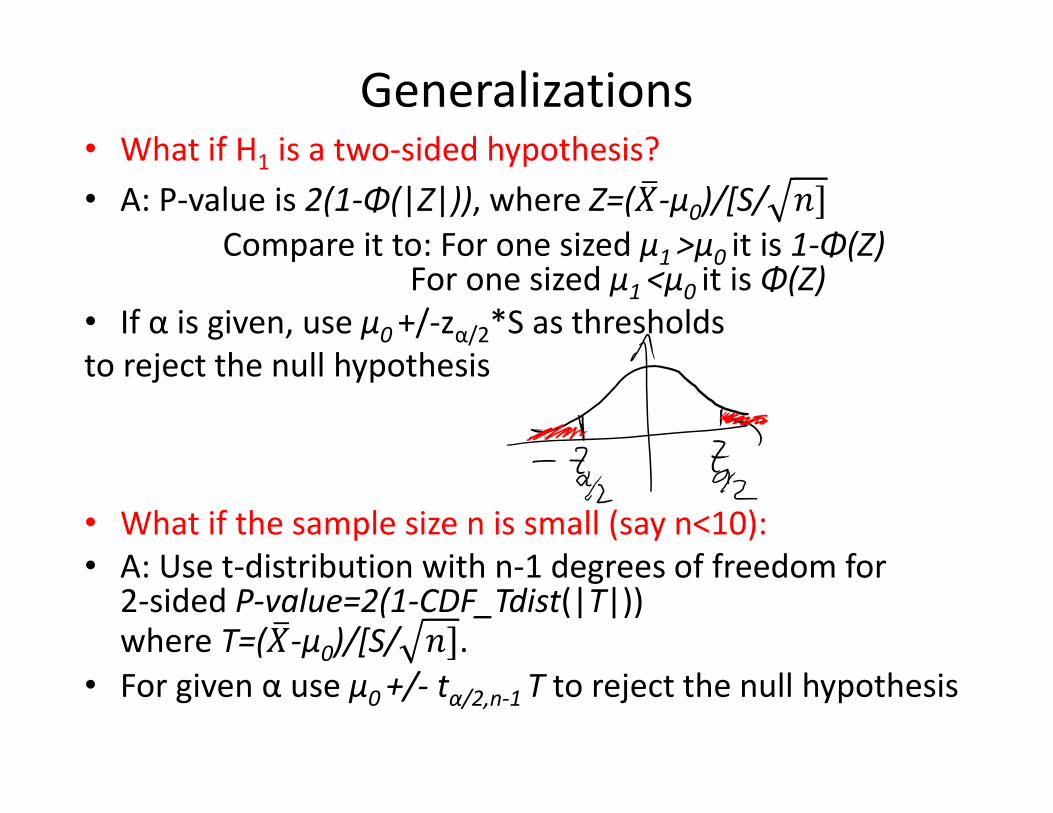
Generalizations• What if H1 is a two‐sided hypothesis? • A: P‐value is 2(1‐Φ(|Z|)), where Z=( ‐μ0)/[S/
Compare it to: For one sized μ1 >μ0 it is 1‐Φ(Z)For one sized μ1 <μ0 it is Φ(Z)
• If α is given, use μ0 +/‐zα/2*S as thresholdsto reject the null hypothesis
• What if the sample size n is small (say n<10):• A: Use t‐distribution with n‐1 degrees of freedom for2‐sided P‐value=2(1‐CDF_Tdist(|T|))where T=( ‐μ0)/[S/ .
• For given α use μ0 +/‐ tα/2,n‐1 T to reject the null hypothesis
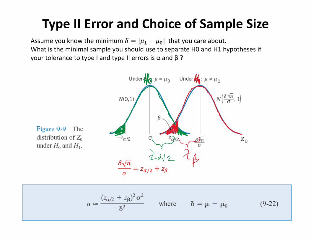
Type II Error and Choice of Sample SizeAssume you know the minimum 𝛿 |𝜇 𝜇 | that you care about. What is the minimal sample you should use to separate H0 and H1 hypotheses if your tolerance to type I and type II errors is α and β ?
𝛿 𝑛𝜎 𝑧 / 𝑧
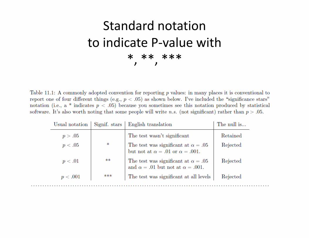
Standard notation to indicate P‐value with
*, **, ***
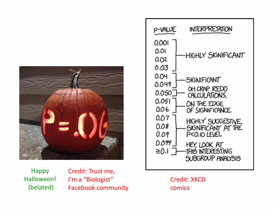
Credit: XKCD comics
Happy Halloween!(belated)
Credit: Trust me,I’m a “Biologist”Facebook community

Credit: XKCD comics
Hypothesis testing:two samples
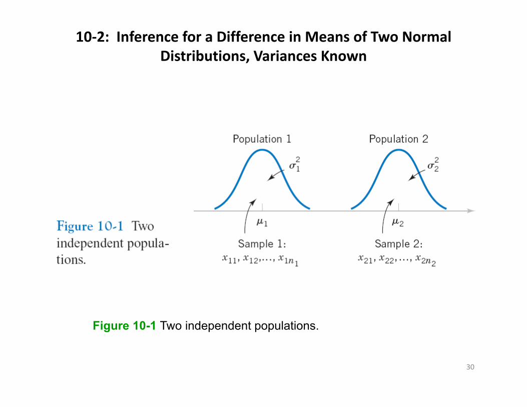
10‐2: Inference for a Difference in Means of Two Normal Distributions, Variances Known
Figure 10-1 Two independent populations.
30
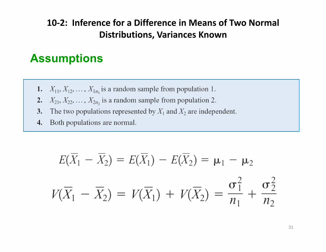
10‐2: Inference for a Difference in Means of Two Normal Distributions, Variances Known
Assumptions
31
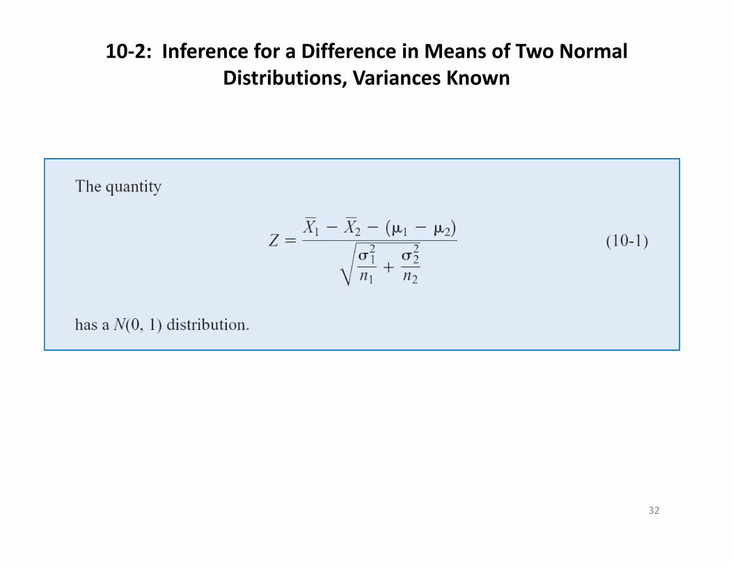
10‐2: Inference for a Difference in Means of Two Normal Distributions, Variances Known
32
10‐2: Inference for a Difference in Means of Two Normal Distributions, Variances Known
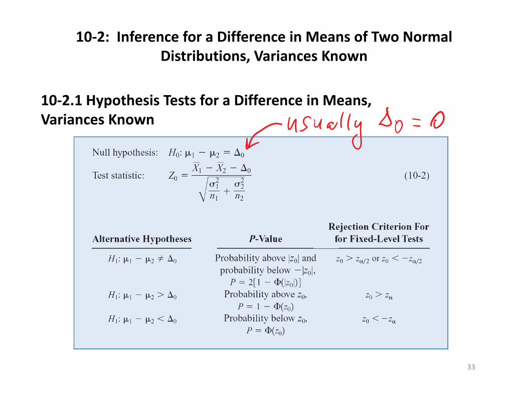
10‐2.1 Hypothesis Tests for a Difference in Means, Variances Known
33
22
21 Case 2:
34
2
22
1
21
021*0
nS
nS
XXT
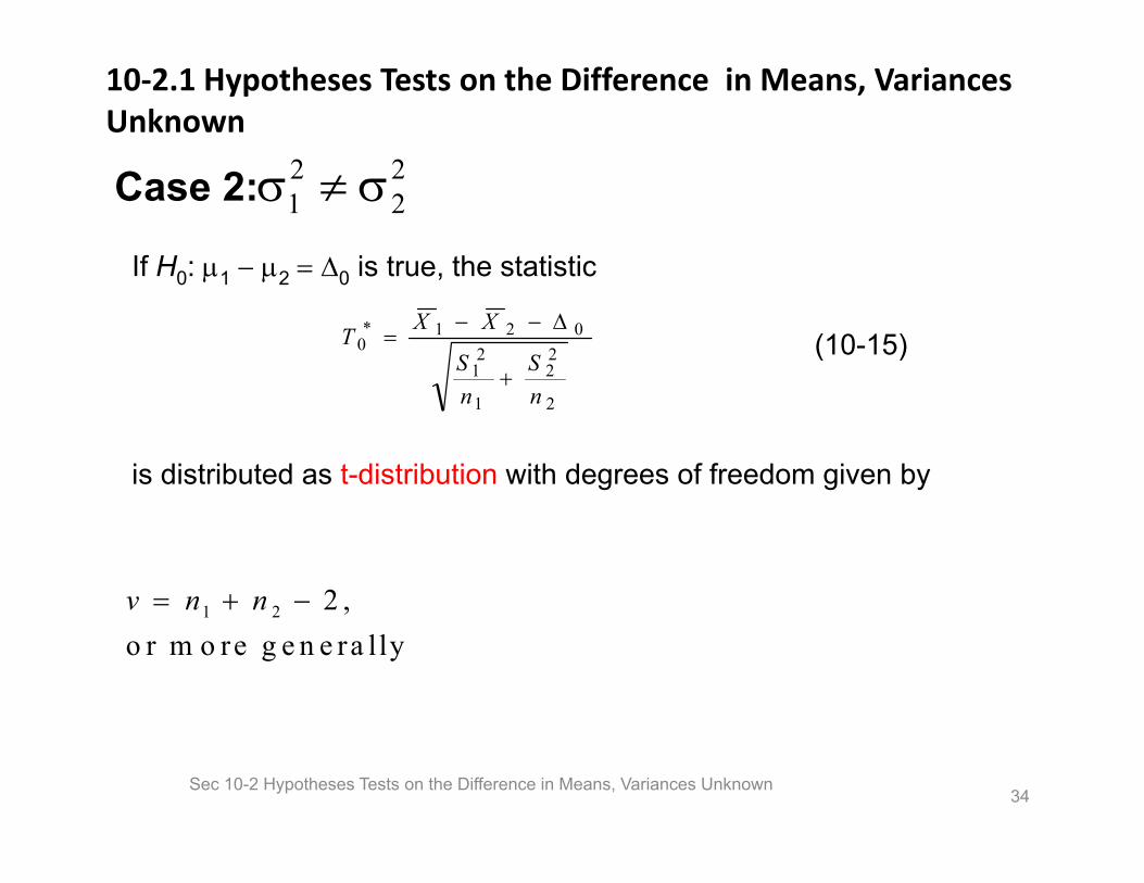
If H0: 1 2 0 is true, the statistic
is distributed as t-distribution with degrees of freedom given by
10‐2.1 Hypotheses Tests on the Difference in Means, Variances Unknown
(10-15)
Sec 10-2 Hypotheses Tests on the Difference in Means, Variances Unknown
1 2 2 , o r m o re g e n e ra llyv n n
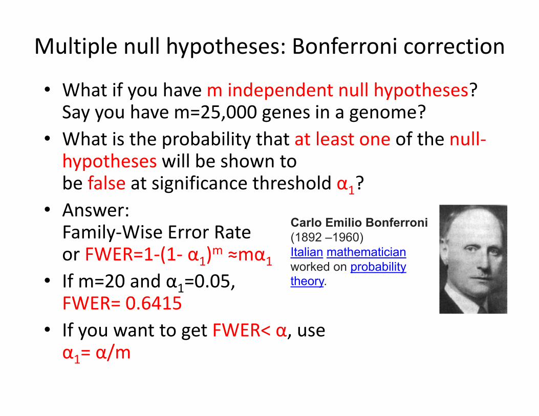
Multiple null hypotheses: Bonferroni correction
• What if you have m independent null hypotheses? Say you have m=25,000 genes in a genome?
• What is the probability that at least one of the null‐hypotheses will be shown to be false at significance threshold α1?
• Answer: Family‐Wise Error Rate or FWER=1‐(1‐ α1)m ≈mα1
• If m=20 and α1=0.05, FWER= 0.6415
• If you want to get FWER< α, use α1= α/m
Carlo Emilio Bonferroni(1892 –1960)Italian mathematicianworked on probability theory.
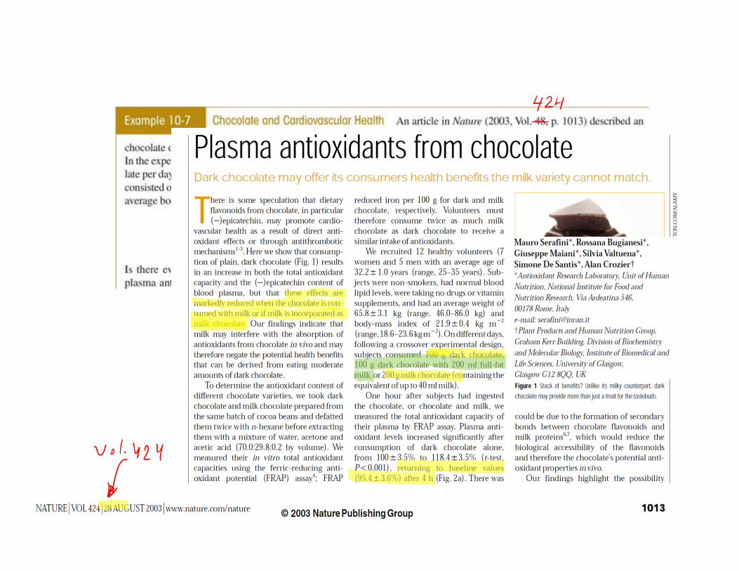
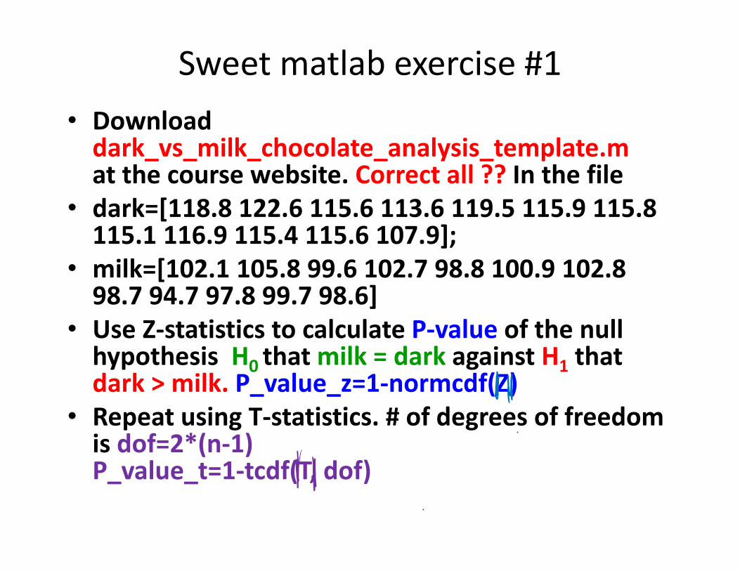
Sweet matlab exercise #1• Download dark_vs_milk_chocolate_analysis_template.mat the course website. Correct all ?? In the file
• dark=[118.8 122.6 115.6 113.6 119.5 115.9 115.8 115.1 116.9 115.4 115.6 107.9];
• milk=[102.1 105.8 99.6 102.7 98.8 100.9 102.8 98.7 94.7 97.8 99.7 98.6]
• Use Z‐statistics to calculate P‐value of the null hypothesis H0 that milk = dark against H1 that dark > milk. P_value_z=1‐normcdf(Z)
• Repeat using T‐statistics. # of degrees of freedom is dof=2*(n‐1)P_value_t=1‐tcdf(T, dof)
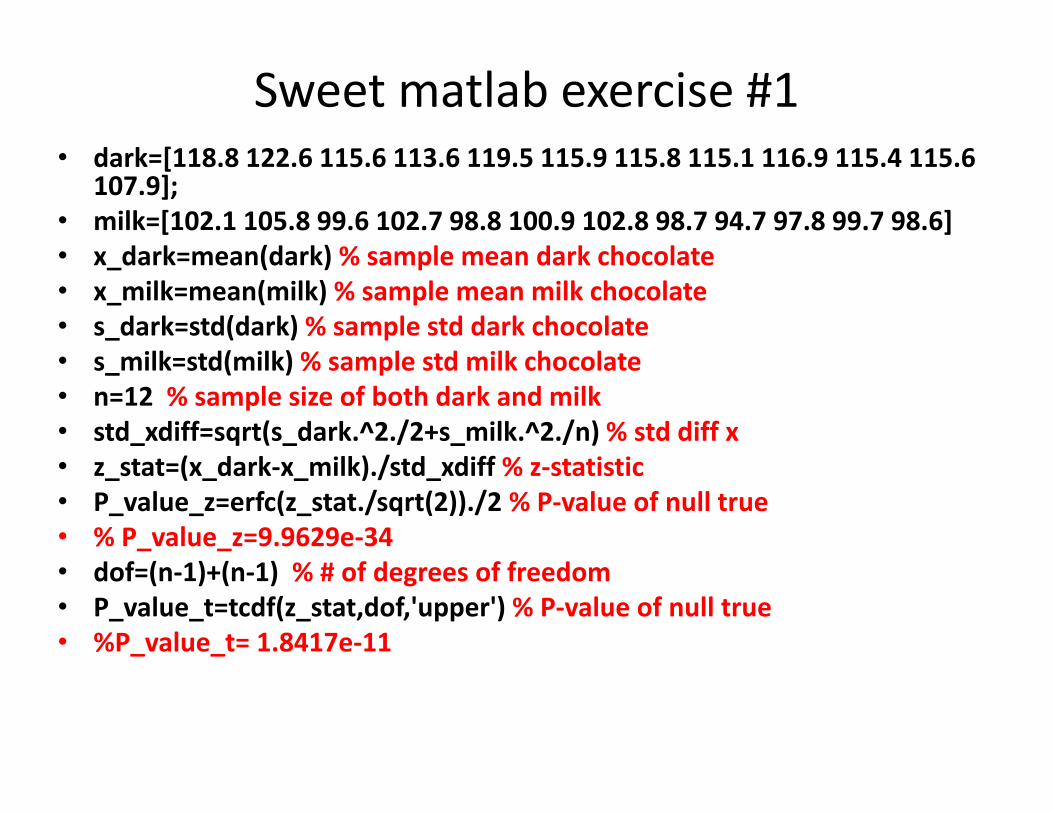
Sweet matlab exercise #1• dark=[118.8 122.6 115.6 113.6 119.5 115.9 115.8 115.1 116.9 115.4 115.6
107.9];• milk=[102.1 105.8 99.6 102.7 98.8 100.9 102.8 98.7 94.7 97.8 99.7 98.6]• x_dark=mean(dark) % sample mean dark chocolate• x_milk=mean(milk) % sample mean milk chocolate• s_dark=std(dark) % sample std dark chocolate• s_milk=std(milk) % sample std milk chocolate• n=12 % sample size of both dark and milk• std_xdiff=sqrt(s_dark.^2./2+s_milk.^2./n) % std diff x• z_stat=(x_dark‐x_milk)./std_xdiff % z‐statistic • P_value_z=erfc(z_stat./sqrt(2))./2 % P‐value of null true• % P_value_z=9.9629e‐34• dof=(n‐1)+(n‐1) % # of degrees of freedom• P_value_t=tcdf(z_stat,dof,'upper') % P‐value of null true• %P_value_t= 1.8417e‐11
Credit: XKCD comics
Top Related