


γλώσσες
Σελίδες
Νομικός

14th European Turbulence Conference, Sep. 1-4 2013, Lyon, France
Direct Numerical Simulation of Turbulent Wall Flows at Constant Power Input
Y. Hasegawa1, B. Frohnapfel2 & M. Quadrio3
1Institute of Industrial Science, The University of Tokyo2Institute of Fluid Mechanics, Karlsruhe Institute of Technology
3Dept. Aerospace. Eng., Polytechnic Institute of Milan
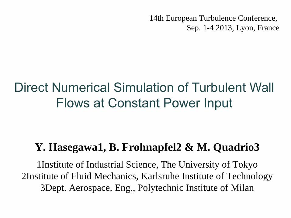
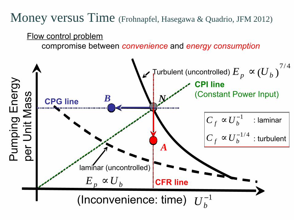
Flow Condition in Numerical Simulation
Length: L
XXPump
Depth:
€
2δ€
∆P = τwL /δPressure drop:
€
UBBulk velocity:
wall friction
Constant Flow Rate (CFR): pressure drop (wall friction) fluctuates in time
Successful Control Reduction of pressure drop
Constant Pressure Gradient (CPG): The flow rate fluctuates in time
Successful Control Increase of flow rate
Conventional approaches
Example: Channel flow
control,obstacles, roughness etc.
Are they the only available options ? No !
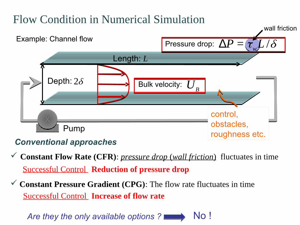
CPI line(Constant Power Input)
Money versus Time (Frohnapfel, Hasegawa & Quadrio, JFM 2012)
(Inconvenience: time)
€
U b−1
Pum
pin
g E
ner
gy
per
Un
it M
ass
€
C f ∝U b−1
C f ∝U b−1/ 4
: laminar
: turbulent
€
E p ∝ U b( )7/ 4
Turbulent (uncontrolled)
€
E p ∝U b
laminar (uncontrolled)
N
A
CFR line
BCPG line
Flow control problemcompromise between convenience and energy consumption
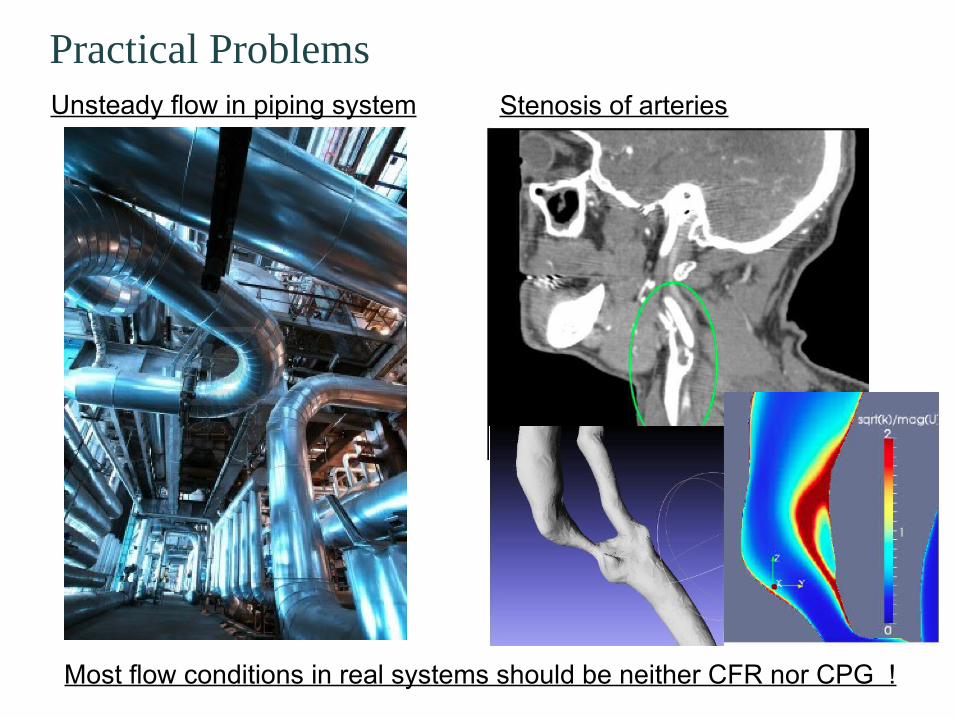
Practical ProblemsUnsteady flow in piping system Stenosis of arteries
Most flow conditions in real systems should be neither CFR nor CPG !
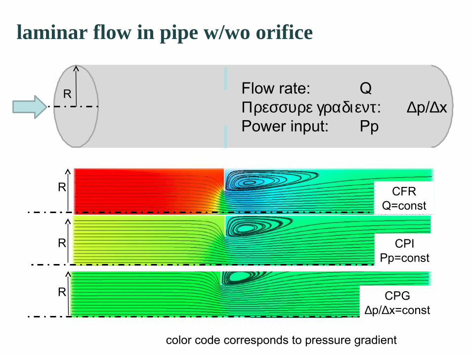
R Flow rate: QΠρεσσυρε γραδιεντ: ∆p/∆xPower input: Pp
color code corresponds to pressure gradient
R CFRQ=const
R CPIPp=const
R CPG∆p/∆x=const
laminar flow in pipe w/wo orifice
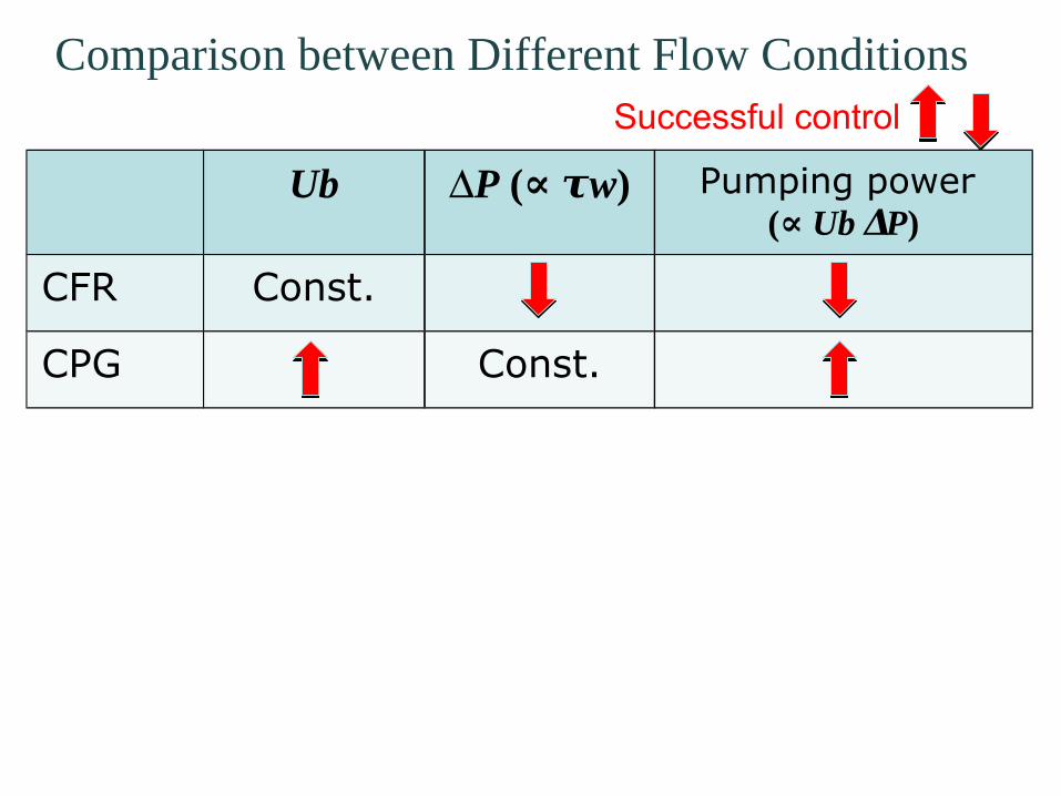
Comparison between Different Flow Conditions
Ub P Δ ( w∝ τ ) Pumping power ( Ub P∝ Δ )
CFR Const.
CPG Const.
Successful control
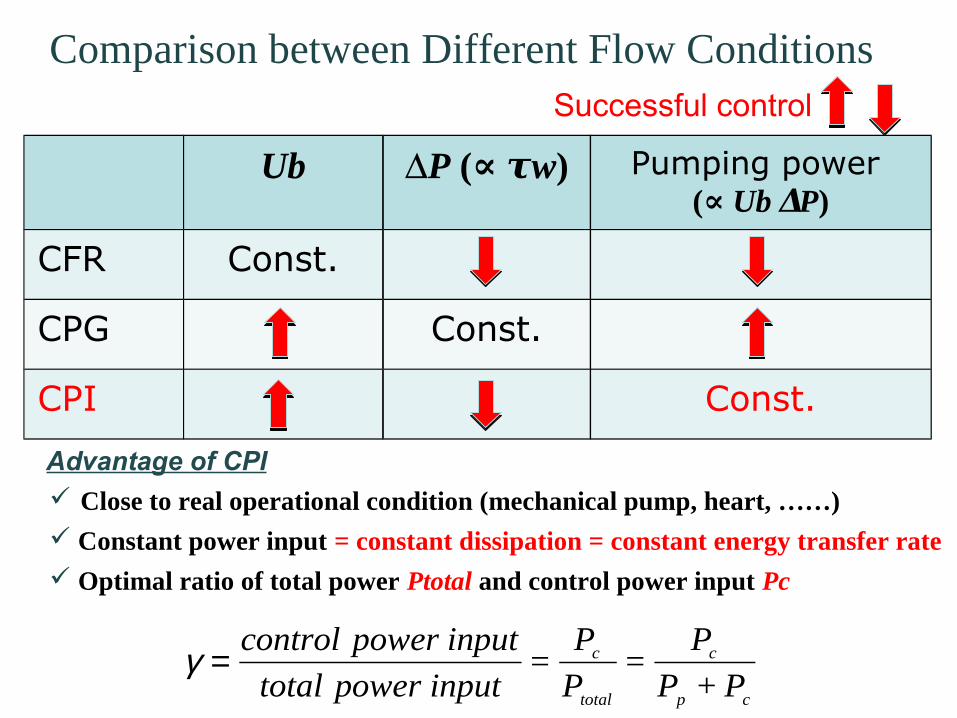
Comparison between Different Flow Conditions
Ub P Δ ( w∝ τ ) Pumping power ( Ub P∝ Δ )
CFR Const.
CPG Const.
CPI Const.
Successful control
Close to real operational condition (mechanical pump, heart, ……) Constant power input = constant dissipation = constant energy transfer rate Optimal ratio of total power Ptotal and control power input Pc
Advantage of CPI
€
γ =control power input
total power input=
Pc
Ptotal
=Pc
Pp + Pc

Introduction to CPI concept
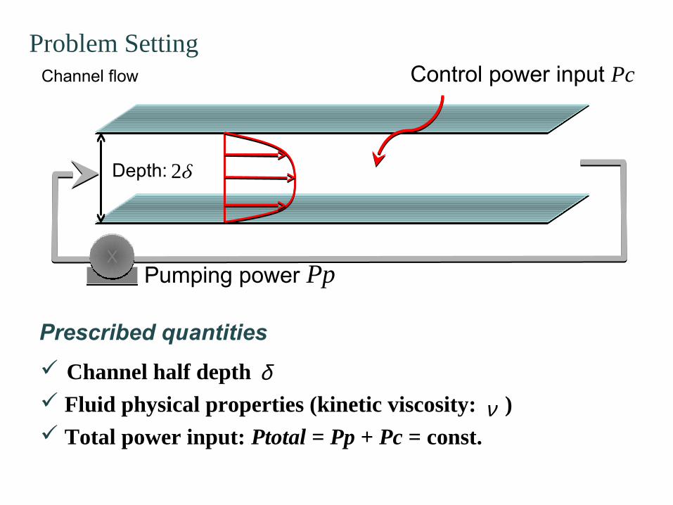
Problem Setting
XXPumping power Pp
Depth:
€
2δ
Channel flow Control power input Pc
Channel half depth Fluid physical properties (kinetic viscosity: ) Total power input: Ptotal = Pp + Pc = const.
Prescribed quantities
€
δ
€
ν
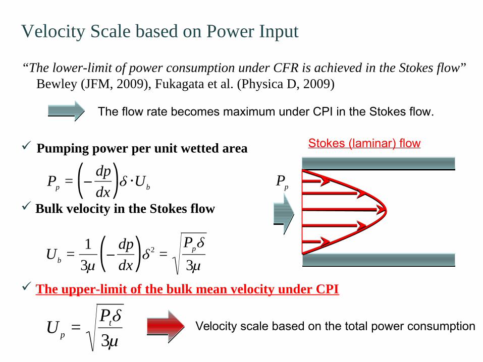
Velocity Scale based on Power Input
“The lower-limit of power consumption under CFR is achieved in the Stokes flow” Bewley (JFM, 2009), Fukagata et al. (Physica D, 2009)
The flow rate becomes maximum under CPI in the Stokes flow.
Pumping power per unit wetted area
Bulk velocity in the Stokes flow
€
Pp = −dp
dx ⎛ ⎝
⎞ ⎠δ ⋅Ub
€
Ub =1
3μ−
dp
dx ⎛ ⎝
⎞ ⎠δ 2 =
Ppδ3μ
€
U p =Ptδ3μ
The upper-limit of the bulk mean velocity under CPI
Velocity scale based on the total power consumption
€
Pp
Stokes (laminar) flow
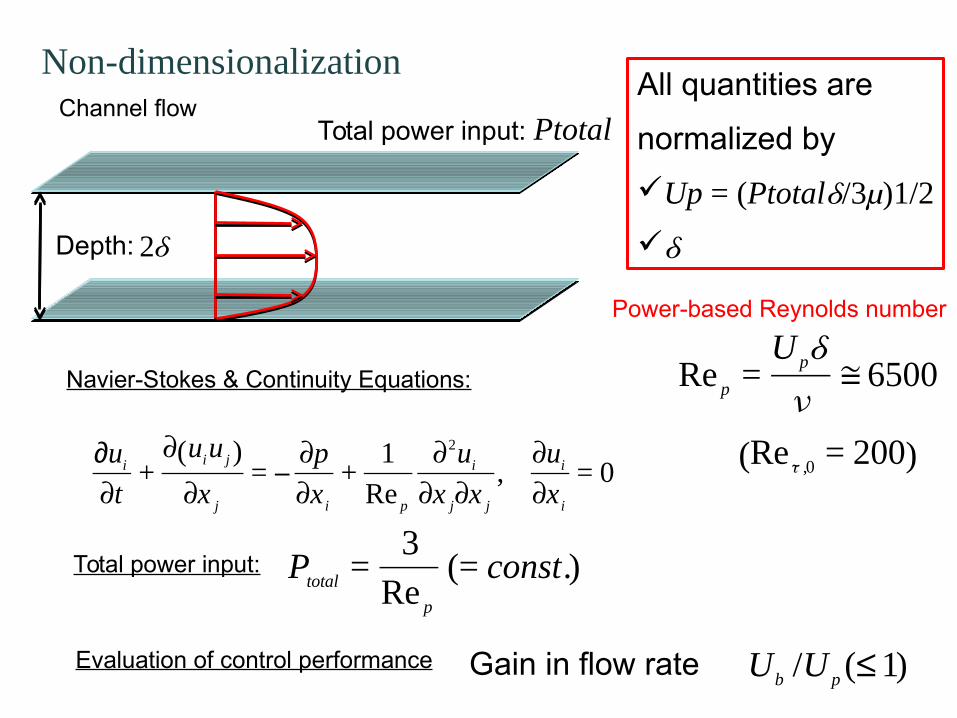
Non-dimensionalization
Depth:
€
2δ
Channel flowAll quantities are
normalized by
Up = (Ptotalδ/3μ)1/2
δ
Total power input: Ptotal
Navier-Stokes & Continuity Equations:
€
∂ui
∂t+
∂ uiu j( )
∂x j
= −∂p
∂x i
+1
Re p
∂2ui
∂x j∂x j
,∂ui
∂x i
= 0
€
Re p =U pδν
≅ 6500
Evaluation of control performance
€
Ub /U p ≤ 1( )Gain in flow rate
Power-based Reynolds number
Total power input:
€
Ptotal =3
Re p
= const.( )€
Reτ ,0 = 200( )
Uncontrolled flow under CPI
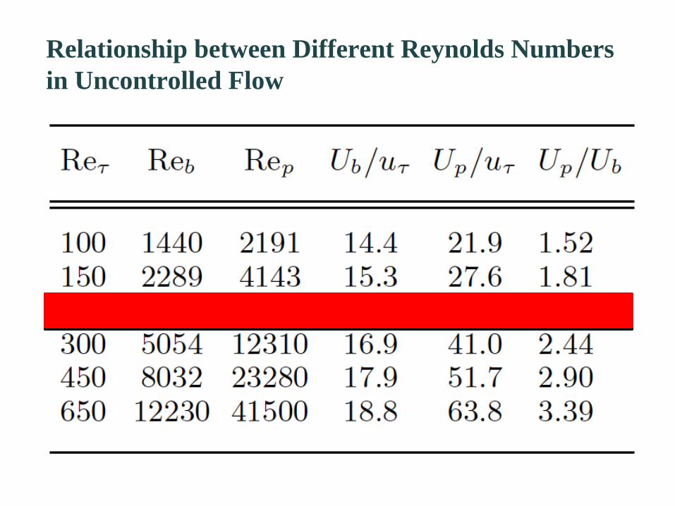
Relationship between Different Reynolds Numbers in Uncontrolled Flow
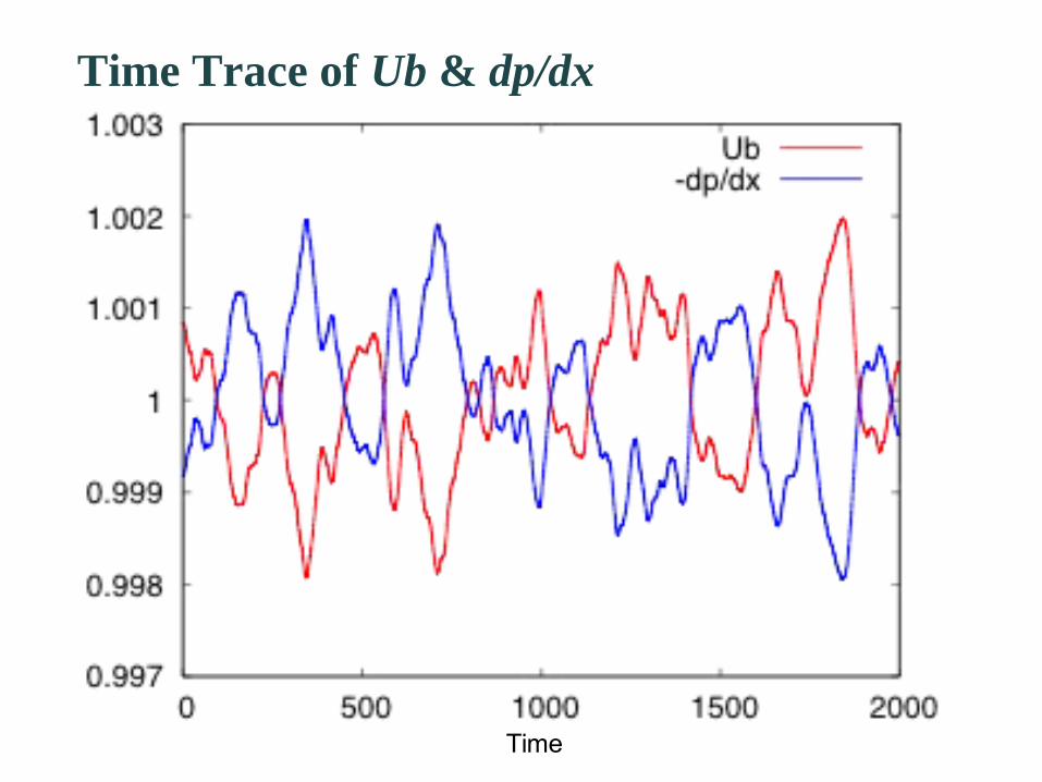
Time
Time Trace of Ub & dp/dx
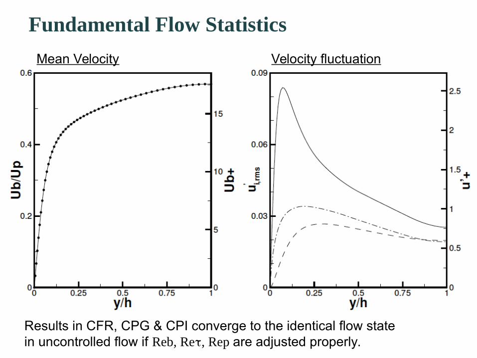
Fundamental Flow Statistics
Mean Velocity Velocity fluctuation
Results in CFR, CPG & CPI converge to the identical flow state in uncontrolled flow if Reb, Re , Rep τ are adjusted properly.
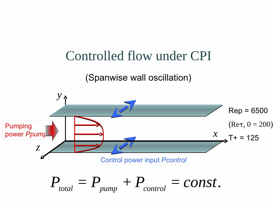
Controlled flow under CPI
Rep = 6500
(Re , 0 = 200τ )
T+ = 125
(Spanwise wall oscillation)
x
y
zControl power input Pcontrol
Pumping power Ppump
€
Ptotal = Ppump + Pcontrol = const.
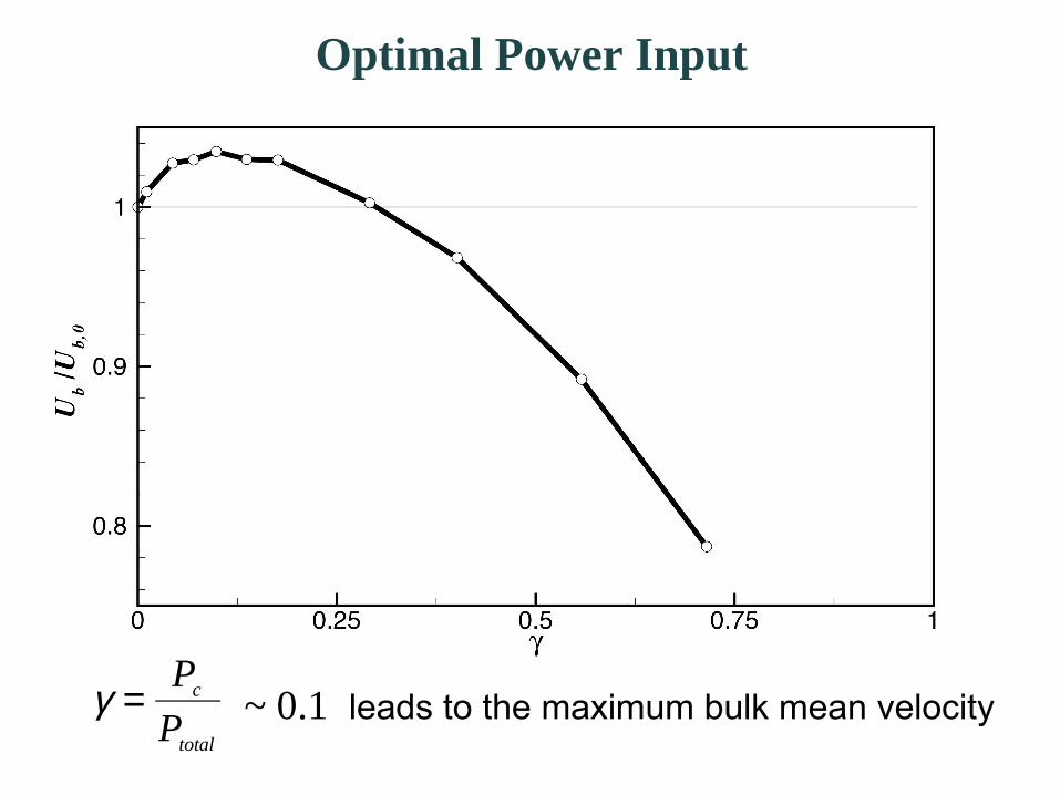
Optimal Power Input
€
γ =Pc
Ptotal
~ 0.1 leads to the maximum bulk mean velocity
Conclusions Constant power input (CPI) condition is proposed as a flow condition
alternative to conventional CFR and CPG close to real operational condition power input (= energy transfer rate = dissipation) is kept constant optimal ratio of total power input and control power input
CPI condition is first implemented in DNS of wall turbulence Power-based velocity scale: Up dimensionless total power input: 3/Rep
CPI simulation successfully run for the uncontrolled and controlled flows.
Uncontrolled flow under CPI is essentially same as those under CFR and CPG.
In the controlled flow, the maximum Ub is obtained when is γaround 10%.
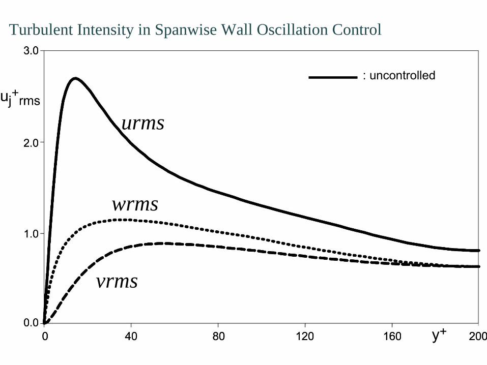
Turbulent Intensity in Spanwise Wall Oscillation Control
: uncontrolled
urms
wrms
vrms
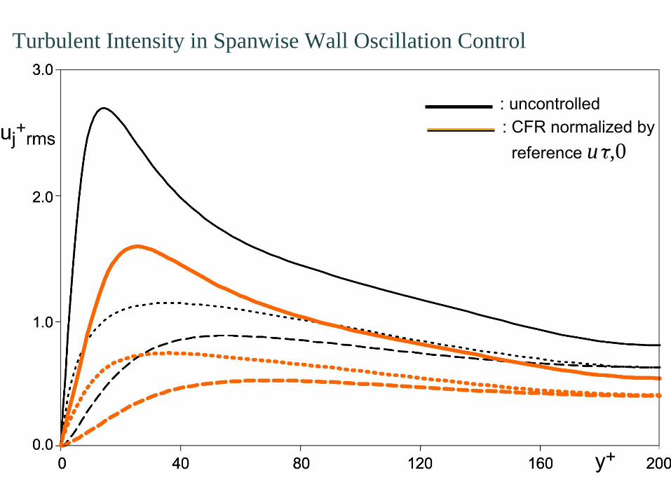
Turbulent Intensity in Spanwise Wall Oscillation Control
: uncontrolled: CFR normalized by
reference uτ,0
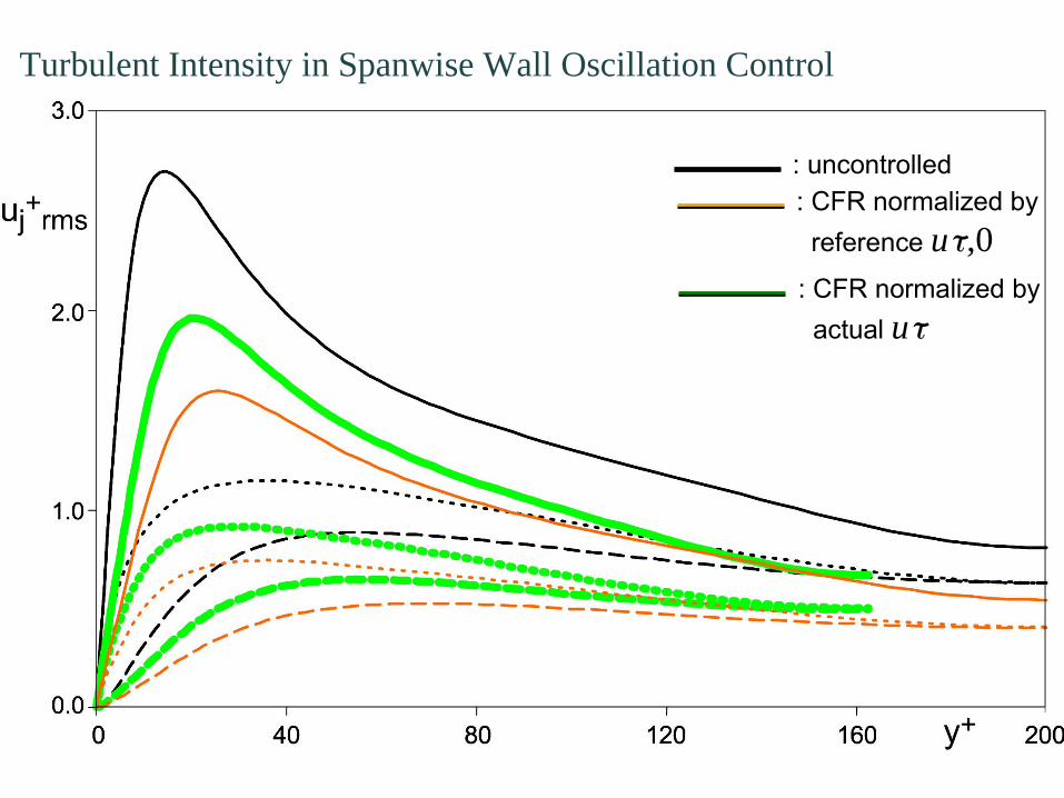
Turbulent Intensity in Spanwise Wall Oscillation Control
: uncontrolled: CFR normalized by
reference uτ,0 : CFR normalized by
actual uτ
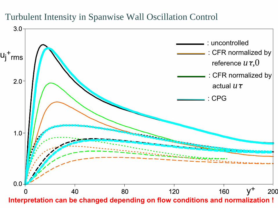
Turbulent Intensity in Spanwise Wall Oscillation Control
: uncontrolled: CFR normalized by
reference uτ,0 : CFR normalized by
actual uτ : CPG
Interpretation can be changed depending on flow conditions and normalization !
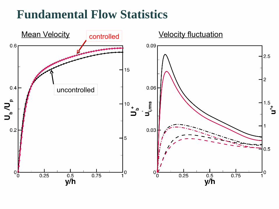
Fundamental Flow Statistics
Mean Velocity Velocity fluctuation
uncontrolled
controlled
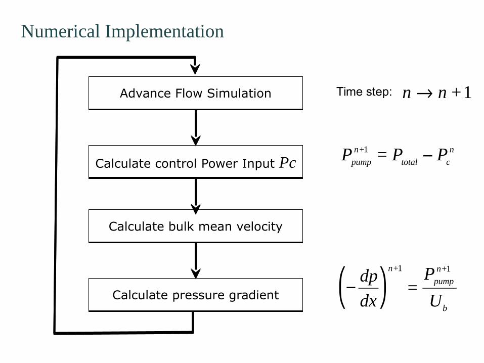
Numerical Implementation
Advance Flow SimulationAdvance Flow Simulation
Calculate control Power Input PcCalculate control Power Input Pc
Calculate bulk mean velocityCalculate bulk mean velocity
Calculate pressure gradientCalculate pressure gradient
€
Ppump
n+1 = Ptotal − Pc
n
€
−dp
dx ⎛ ⎝
⎞ ⎠
n+1
=Ppump
n+1
Ub
€
n→ n +1Time step:
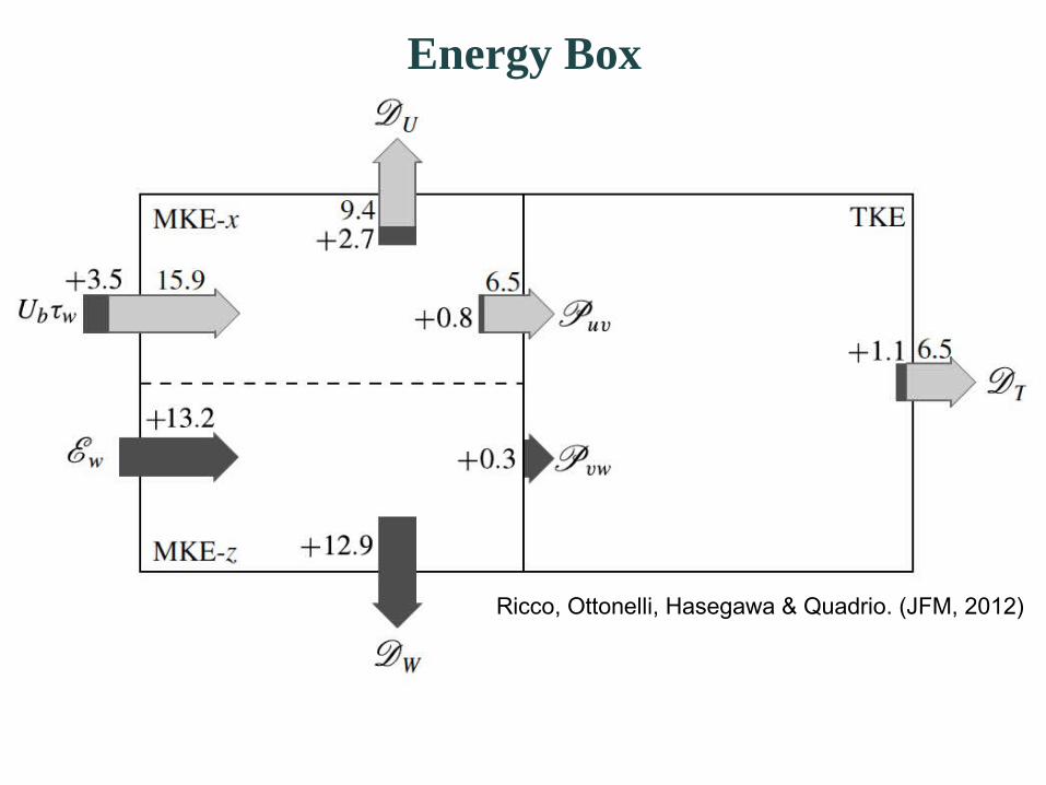
Energy Box
Ricco, Ottonelli, Hasegawa & Quadrio. (JFM, 2012)
Top Related