1

1

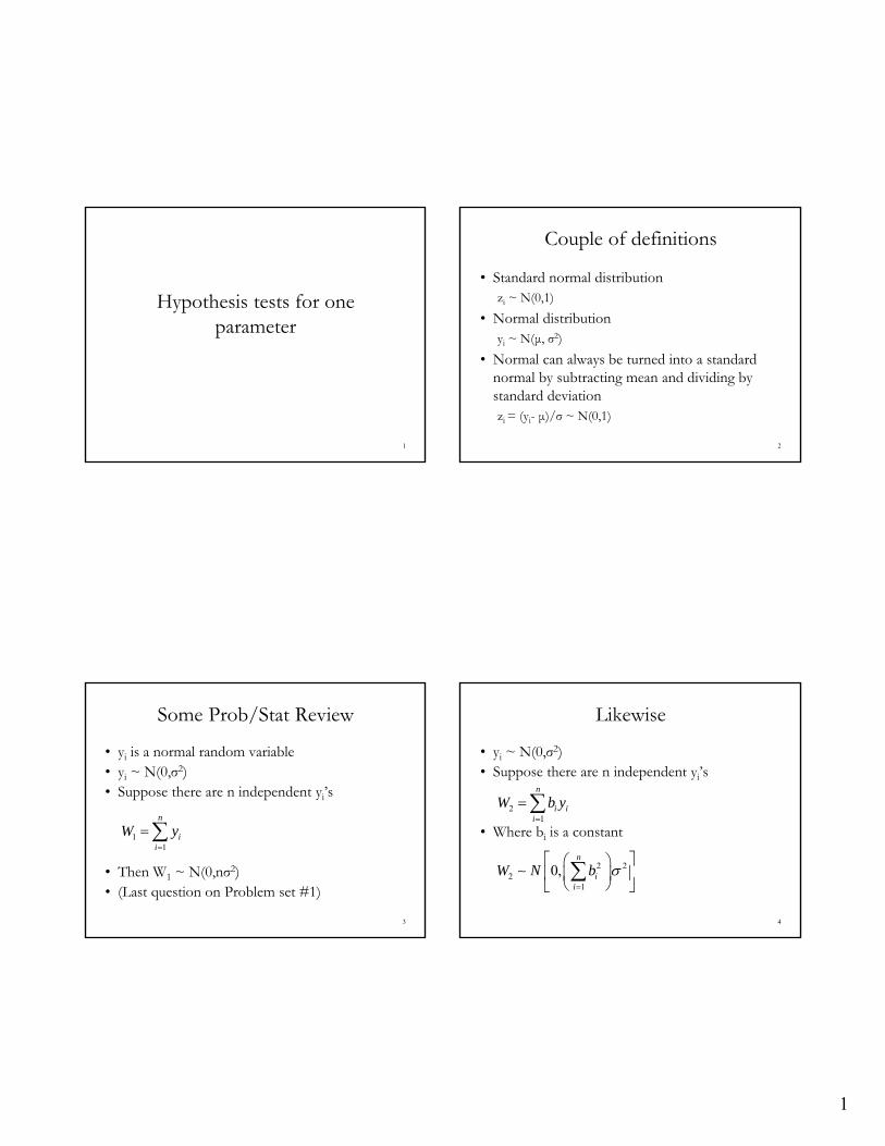
Hypothesis tests for one parameter

Couple of definitions

• Standard normal distributionzi ~ N(0,1)

• Normal distributionyi ~ N(μ, σ2)

• Normal can always be turned into a standard normal by subtracting mean and dividing by standard deviationzi = (yi- μ)/σ ~ N(0,1)

2

3

Some Prob/Stat Review

• yi is a normal random variable• yi ~ N(0,σ2)• Suppose there are n independent yi’s

• Then W1 ~ N(0,nσ2)• (Last question on Problem set #1)

11

n

ii

W y

4

Likewise

• yi ~ N(0,σ2)• Suppose there are n independent yi’s

• Where bi is a constant

21

n

i ii

W b y

2 22

1

0,n

ii

W N b

2

5

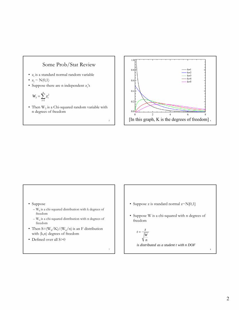
Some Prob/Stat Review

• zi is a standard normal random variable• zi ~ N(0,1)• Suppose there are n independent zi’s

• Then W3 is a Chi-squared random variable with n degrees of freedom

23

1

n

ii

W z

6[In this graph, K is the degrees of freedom]

7

• Suppose– Wk is a chi-squared distribution with k degrees of

freedom

– Wn is a chi-squared distribution with n degrees of freedom

• Then S=(Wk/K)/(Wn/n) is an F distribution with (k,n) degrees of freedom

• Defined over all S>0

8

• Suppose z is standard normal z~N[0,1]

• Suppose W is a chi-squared with n degrees of freedom

zt

Wn

is distributed as a student t with n DOF

3

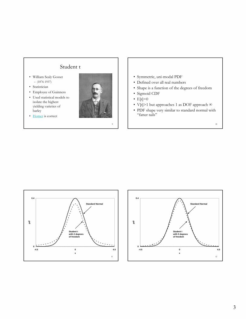
Student t

• William Sealy Gosset– (1876-1937)

• Statistician

• Employee of Guinness

• Used statistical models to isolate the highest yielding varieties of barley

• Homer is correct

9 10

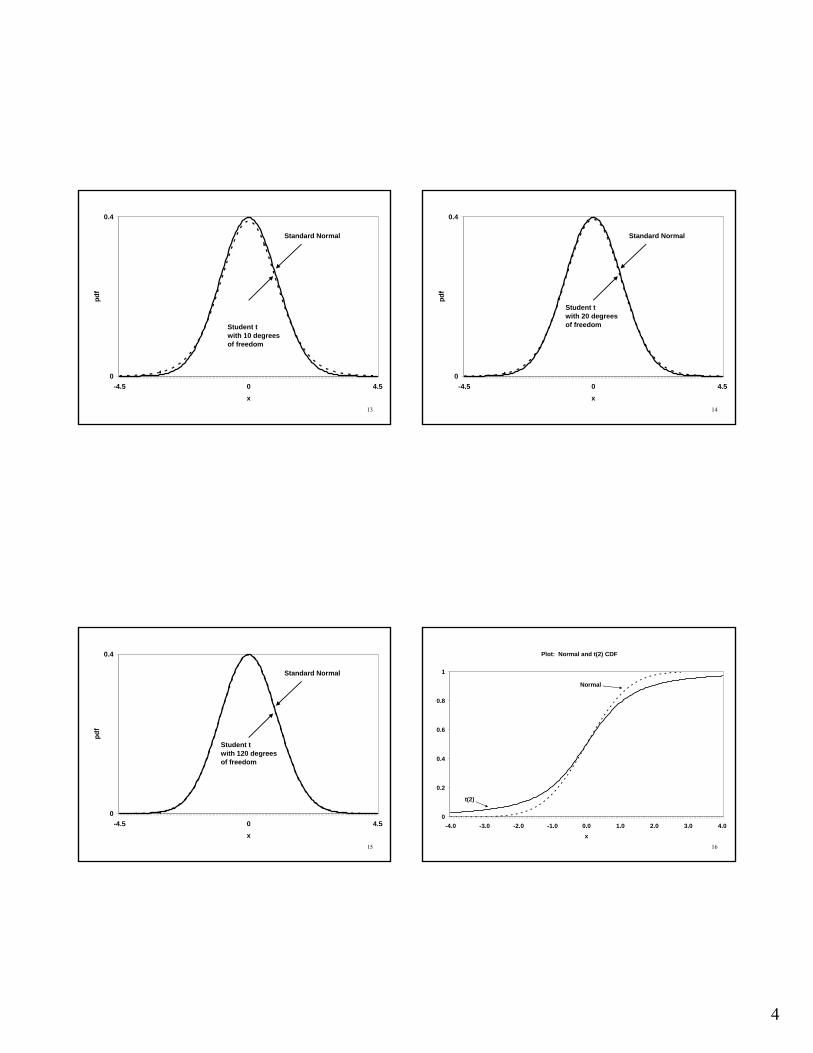
• Symmetric, uni-modal PDF• Defined over all real numbers• Shape is a function of the degrees of freedom• Sigmoid CDF • E[t]=0• V[t]>1 but approaches 1 as DOF approach ∞• PDF shape very similar to standard normal with

“fatter tails”

11

0

0.4

-4.5 0 4.5

x

pd

f

Standard Normal

Student twith 2 degreesof freedom

12

0

0.4

-4.5 0 4.5

x

pd

f

Standard Normal

Student twith 5 degreesof freedom

4

13

0

0.4

-4.5 0 4.5

x

pd

f

Standard Normal

Student twith 10 degreesof freedom

14

0

0.4

-4.5 0 4.5

x

pd

f

Standard Normal

Student twith 20 degreesof freedom

15

0

0.4

-4.5 0 4.5

x

pd

f

Standard Normal

Student twith 120 degreesof freedom

16

Plot: Normal and t(2) CDF

0

0.2

0.4

0.6

0.8

1

-4.0 -3.0 -2.0 -1.0 0.0 1.0 2.0 3.0 4.0

x

Normal

t(2)

5

17

Plot: Normal and t(10) CDF

0

0.2

0.4

0.6

0.8

1

-4.0 -3.0 -2.0 -1.0 0.0 1.0 2.0 3.0 4.0

x

Normal

t(10)

18

Plot: Normal and t(100) CDF

0

0.2

0.4

0.6

0.8

1

-4.0 -3.0 -2.0 -1.0 0.0 1.0 2.0 3.0 4.0

x

Normal

t(100)

19

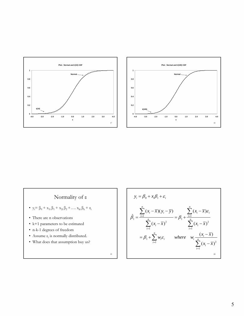
Normality of ε

• yi= β0 + x1i β1 + x2i β2 +…. xki βk + εi

• There are n observations

• k+1 parameters to be estimated

• n-k-1 degrees of freedom

• Assume εi is normally distributed.

• What does that assumption buy us?

20

0 1i i iy x

1 11 1

2 2

1 1

121

1

( )( ) ( )ˆ

( ) ( )

( )

( )

n n

i i i ii i

n n

i ii i

ni

i i i ni

ii

x x y y x x

x x x x

x xw where w

x x

6

21

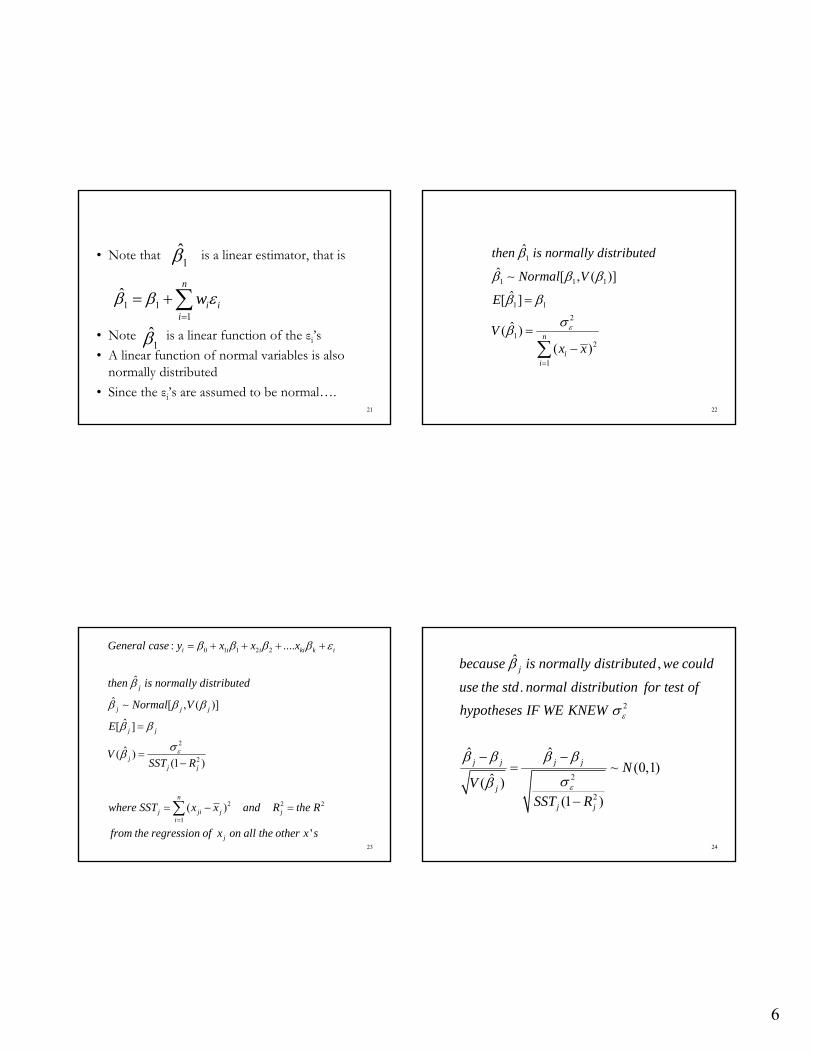
• Note that is a linear estimator, that is

• Note is a linear function of the εi’s

• A linear function of normal variables is also normally distributed

• Since the εi’s are assumed to be normal….

1̂

1 11

ˆn

i ii

w

1̂

22

1

1 1 1

1 1

2

12

1

ˆ

ˆ [ , ( )]

ˆ[ ]

ˆ( )( )

n

ii

then is normally distributed

Normal V

E

Vx x

23

0 1 1 2 2

2

2

2 2 2

1

: ....

ˆ

ˆ [ , ( )]

ˆ[ ]

ˆ( )(1 )

( )

'

i i i ki k i

j

j j j

j j

jj j

n

j ji j ji

j

General case y x x x

then is normally distributed

Normal V

E

VSST R

where SST x x and R the R

from the regression of x on all the other x s

24

2

2

2

ˆ ,

.

ˆ ˆ~ (0,1)

ˆ( )(1 )

j

j j j j

j

j j

because is normally distributed we could

use the std normal distribution for test of

hypotheses IF WE KNEW

NV

SST R

7

25

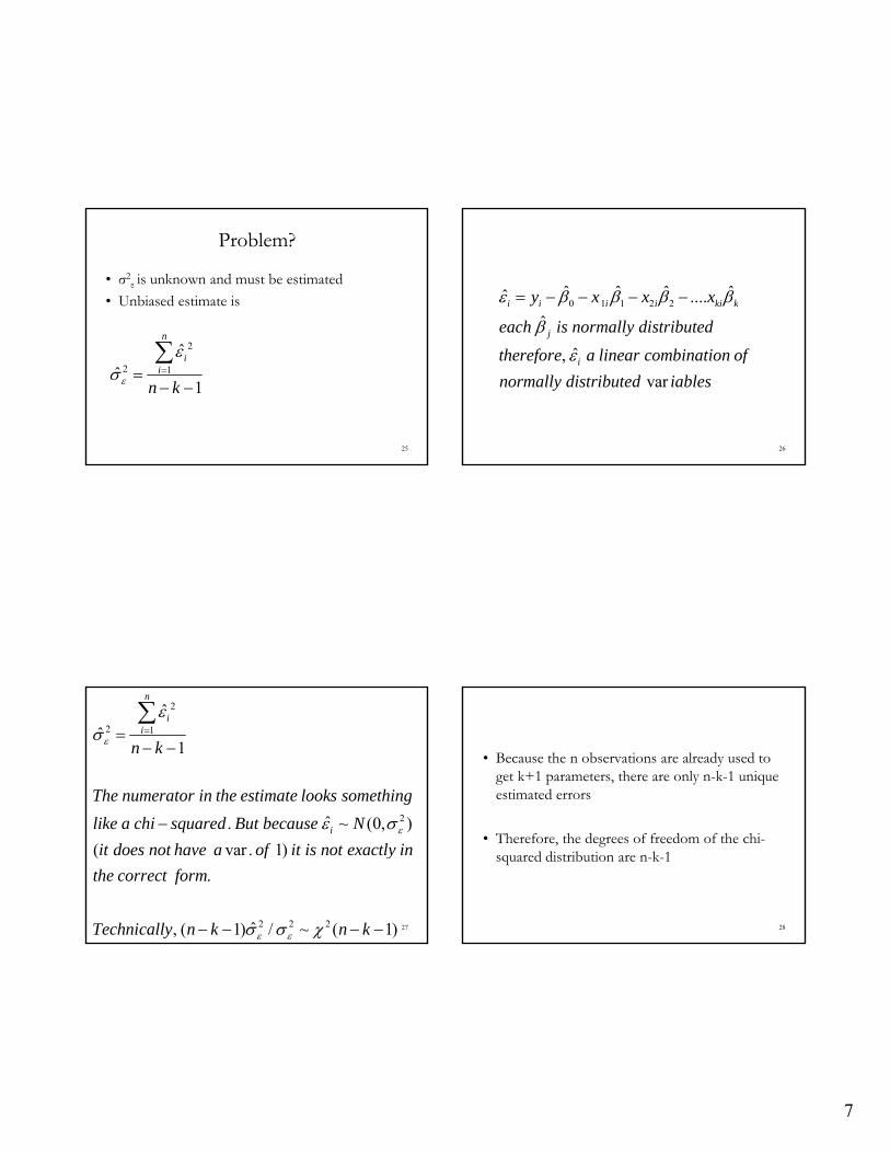
Problem?

• σ2ε is unknown and must be estimated

• Unbiased estimate is

2

2 1

ˆˆ

1

n

ii

n k

26

0 1 1 2 2ˆ ˆ ˆ ˆˆ ....

ˆ

ˆ,

var

i i i i ki k

j

i

y x x x

each is normally distributed

therefore a linear combination of

normally distributed iables

27

2

2 1

2

2 2 2

ˆˆ

1

ˆ. ~ (0, )

( var . 1)

.

ˆ, ( 1) / ~ ( 1)

n

ii

i

n k

The numerator in the estimate looks something

like a chi squared But because N

it does not have a of it is not exactly in

the correct form

Technically n k n k

28

• Because the n observations are already used to get k+1 parameters, there are only n-k-1 unique estimated errors

• Therefore, the degrees of freedom of the chi-squared distribution are n-k-1

8

29

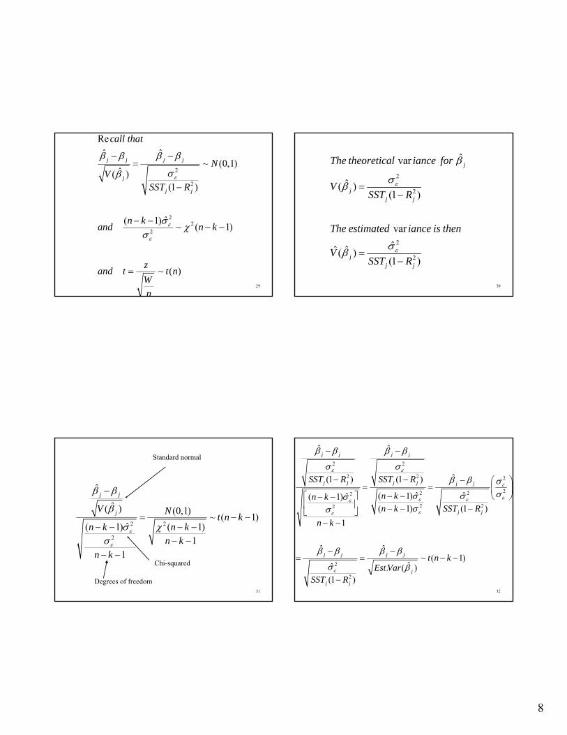
2

2

22

2

Re

ˆ ˆ~ (0,1)

ˆ( )(1 )

ˆ( 1)~ ( 1)

~ ( )

j j j j

j

j j

call that

NV

SST R

n kand n k

zand t t n

Wn

30

2

2

2

2

ˆvar

ˆ( )(1 )

var

ˆˆˆ( )(1 )

j

jj j

jj j

The theoretical iance for

VSST R

The estimated iance is then

VSST R

31

2 2

2

ˆ

ˆ( ) (0,1)~ ( 1)

ˆ( 1) ( 1)1

1

j j

jV Nt n k

n k n kn k

n k

Standard normal

Chi-squared

Degrees of freedom32

2 2

2 2 2

22 22

2 22

2

2

ˆ ˆ

ˆ(1 ) (1 )

ˆ ˆ( 1)ˆ( 1)( 1) (1 )

1

ˆ ˆ~ ( 1)

ˆˆ . ( )(1 )

j j j j

j j j j j j

j j

j j j j

j

j j

SST R SST R

n kn kn k SST R

n k

t n kEst Var

SST R

9

33

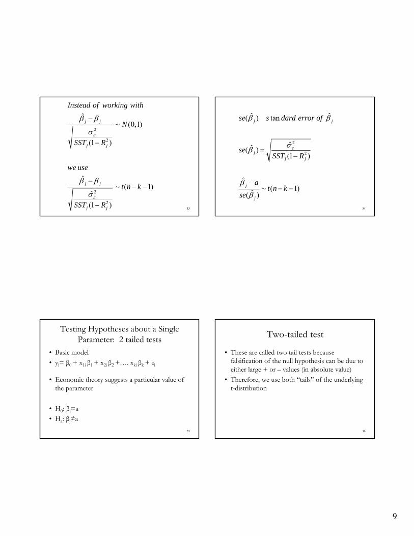
2

2

2

2

ˆ~ (0,1)

(1 )

ˆ~ ( 1)

ˆ

(1 )

j j

j j

j j

j j

Instead of working with

N

SST R

we use

t n k

SST R

34

2

2

ˆ ˆ( ) tan

ˆˆ( )(1 )

ˆ~ ( 1)

ˆ( )

j j

jj j

j

j

se s dard error of

seSST R

at n k

se

35

Testing Hypotheses about a Single Parameter: 2 tailed tests

• Basic model

• yi= β0 + x1i β1 + x2i β2 +…. xki βk + εi

• Economic theory suggests a particular value of the parameter

• H0: βj=a

• Ha: βj≠a

36

Two-tailed test

• These are called two tail tests because falsification of the null hypothesis can be due to either large + or – values (in absolute value)

• Therefore, we use both “tails” of the underlying t-distribution

10

37

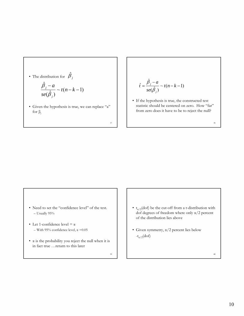
• The distribution for

• Given the hypothesis is true, we can replace “a” for βj

ˆ~ ( 1)

ˆ( )j

j

at n k

se

ˆj

38

• If the hypothesis is true, the constructed test statistic should be centered on zero. How “far” from zero does it have to be to reject the null?

ˆˆ ~ ( 1)

ˆ( )j

j

at t n k

se

39

• Need to set the “confidence level” of the test.– Usually 95%

• Let 1-confidence level = α– With 95% confidence level, α =0.05

• α is the probability you reject the null when it is in fact true …return to this later

40

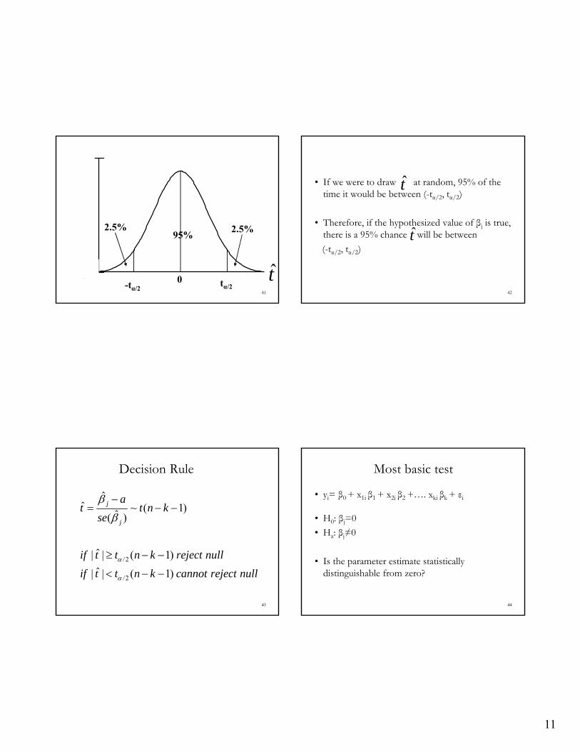
• tα/2(dof) be the cut-off from a t-distribution with dof degrees of freedom where only α/2 percent of the distribution lies above

• Given symmetry, α/2 percent lies below

-tα/2(dof)

11

41

0

0.45

t̂0

2.5% 2.5%95%

-tα/2tα/2

42

• If we were to draw at random, 95% of the time it would be between (-tα/2, tα/2)

• Therefore, if the hypothesized value of βj is true, there is a 95% chance will be between

(-tα/2, tα/2)

t̂

t̂

43

Decision Rule

/2

/2

ˆˆ ~ ( 1)

ˆ( )

ˆ| | ( 1)

ˆ| | ( 1)

j

j

at t n k

se

if t t n k reject null

if t t n k cannot reject null

44

Most basic test

• yi= β0 + x1i β1 + x2i β2 +…. xki βk + εi

• H0: βj=0

• Ha: βj≠0

• Is the parameter estimate statistically distinguishable from zero?

12

45

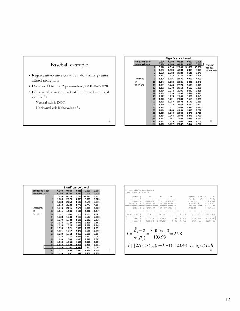
Baseball example

• Regress attendance on wins – do winning teams attract more fans

• Data on 30 teams, 2 parameters, DOF=n-2=28

• Look at table in the back of the book for critical value of t– Vertical axis is DOF

– Horizontal axis is the value of α

46

Significance Levelone-tailed tests 0.100 0.050 0.025 0.010 0.005two-tailed tests 0.200 0.100 0.050 0.020 0.010 1 3.078 6.314 12.706 31.821 63.657

2 1.886 2.920 4.303 6.965 9.9253 1.638 2.353 3.182 4.541 5.8414 1.533 2.132 2.776 3.747 4.604

Degrees 5 1.476 2.015 2.571 3.365 4.032

of 15 1.341 1.753 2.131 2.602 2.947

freedom 16 1.337 1.746 2.120 2.583 2.92117 1.333 1.740 2.110 2.567 2.89818 1.330 1.734 2.101 2.552 2.87819 1.328 1.729 2.093 2.539 2.86120 1.325 1.725 2.086 2.528 2.84521 1.323 1.721 2.080 2.518 2.83122 1.321 1.717 2.074 2.508 2.81923 1.319 1.714 2.069 2.500 2.80724 1.318 1.711 2.064 2.492 2.79725 1.316 1.708 2.060 2.485 2.78726 1.315 1.706 2.056 2.479 2.77927 1.314 1.703 2.052 2.473 2.77128 1.313 1.701 2.048 2.467 2.76329 1.311 1.699 2.045 2.462 2.75630 1.310 1.697 2.042 2.457 2.750

P-valuefor twotailed tests

47

Significance Levelone-tailed tests 0.100 0.050 0.025 0.010 0.005two-tailed tests 0.200 0.100 0.050 0.020 0.010 1 3.078 6.314 12.706 31.821 63.657

2 1.886 2.920 4.303 6.965 9.9253 1.638 2.353 3.182 4.541 5.8414 1.533 2.132 2.776 3.747 4.604

Degrees 5 1.476 2.015 2.571 3.365 4.032

of 15 1.341 1.753 2.131 2.602 2.947

freedom 16 1.337 1.746 2.120 2.583 2.92117 1.333 1.740 2.110 2.567 2.89818 1.330 1.734 2.101 2.552 2.87819 1.328 1.729 2.093 2.539 2.86120 1.325 1.725 2.086 2.528 2.84521 1.323 1.721 2.080 2.518 2.83122 1.321 1.717 2.074 2.508 2.81923 1.319 1.714 2.069 2.500 2.80724 1.318 1.711 2.064 2.492 2.79725 1.316 1.708 2.060 2.485 2.78726 1.315 1.706 2.056 2.479 2.77927 1.314 1.703 2.052 2.473 2.77128 1.313 1.701 2.048 2.467 2.76329 1.311 1.699 2.045 2.462 2.75630 1.310 1.697 2.042 2.457 2.750

48

. * run simple regression

. reg attendance wins Source | SS df MS Number of obs = 30 -------------+------------------------------ F( 1, 28) = 8.89 Model | 606784507 1 606784507 Prob > F = 0.0059 Residual | 1.9110e+09 28 68249360.1 R-squared = 0.2410 -------------+------------------------------ Adj R-squared = 0.2139 Total | 2.5178e+09 29 86819537.6 Root MSE = 8261.3 ------------------------------------------------------------------------------ attendance | Coef. Std. Err. t P>|t| [95% Conf. Interval] -------------+---------------------------------------------------------------- wins | 310.0473 103.9825 2.98 0.006 97.04894 523.0457 _cons | 3095.14 8539.507 0.36 0.720 -14397.25 20587.53 ------------------------------------------------------------------------------

/2

ˆ 310.05 0ˆ 2.98ˆ 103.98( )

ˆ| | | 2.98 | ( 1) 2.048

j

j

at

se

t t n k reject null

13

49

Statistical significance

• When we reject the null hypothesis that H0: βj=0, we say that a variable is “statistically significant”

• Which is short hand for saying the variable is statistically distinguishable from 0

• Statistically insignificant variables are those that we cannot reject the null H0: βj=0

50

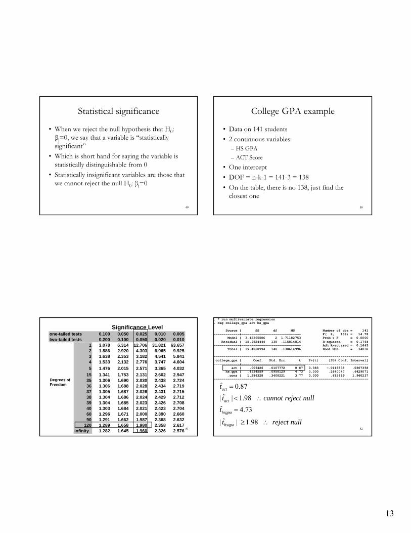
College GPA example

• Data on 141 students

• 2 continuous variables:– HS GPA

– ACT Score

• One intercept

• DOF = n-k-1 = 141-3 = 138

• On the table, there is no 138, just find the closest one

51

Significance Levelone-tailed tests 0.100 0.050 0.025 0.010 0.005two-tailed tests 0.200 0.100 0.050 0.020 0.010 1 3.078 6.314 12.706 31.821 63.657

2 1.886 2.920 4.303 6.965 9.9253 1.638 2.353 3.182 4.541 5.8414 1.533 2.132 2.776 3.747 4.604

Degrees 5 1.476 2.015 2.571 3.365 4.032

of 15 1.341 1.753 2.131 2.602 2.94735 1.306 1.690 2.030 2.438 2.72436 1.306 1.688 2.028 2.434 2.71937 1.305 1.687 2.026 2.431 2.71538 1.304 1.686 2.024 2.429 2.71239 1.304 1.685 2.023 2.426 2.70840 1.303 1.684 2.021 2.423 2.70460 1.296 1.671 2.000 2.390 2.66090 1.291 1.662 1.987 2.368 2.632

120 1.289 1.658 1.980 2.358 2.617infinity 1.282 1.645 1.960 2.326 2.576

Degrees of Freedom

52

. * run multivariate regression

. reg college_gpa act hs_gpa Source | SS df MS Number of obs = 141 -------------+------------------------------ F( 2, 138) = 14.78 Model | 3.42365506 2 1.71182753 Prob > F = 0.0000 Residual | 15.9824444 138 .115814814 R-squared = 0.1764 -------------+------------------------------ Adj R-squared = 0.1645 Total | 19.4060994 140 .138614996 Root MSE = .34032 ------------------------------------------------------------------------------ college_gpa | Coef. Std. Err. t P>|t| [95% Conf. Interval] -------------+---------------------------------------------------------------- act | .009426 .0107772 0.87 0.383 -.0118838 .0307358 hs_gpa | .4534559 .0958129 4.73 0.000 .2640047 .6429071 _cons | 1.286328 .3408221 3.77 0.000 .612419 1.960237 ------------------------------------------------------------------------------ ˆ 0.87

ˆ| | 1.98

ˆ 4.73

ˆ| | 1.98

act

act

hsgpa

hsgpa

t

t cannot reject null

t

t reject null

14

53

Confidence intervals

• The CI represent the 95% most likely values of the parameter βj

• If the hypothesized value “a” (H0: βj=a) is not part of the confidence interval, it is not a likely value and we reject the null

• If interval contains “a” we cannot reject null

• The t-test and CI should provide the same decision – if not, you did something wrong

54

/2 /2

/2

/2

,

ˆ( 1) ( 1)

ˆ( )

ˆ ˆ( ) ( 1)

ˆ ˆ( ) ( 1)

j

j

j j

j j

if the null is true then

at n k t n k

se

which means that

se t n k a

se t n k

Confidence intervals

55

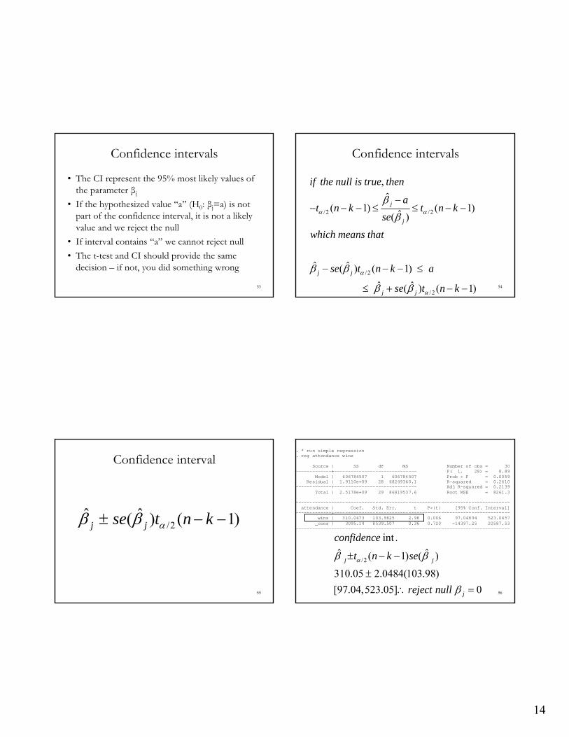
Confidence interval

/2ˆ ˆ( ) ( 1)j jse t n k

56

. * run simple regression

. reg attendance wins Source | SS df MS Number of obs = 30 -------------+------------------------------ F( 1, 28) = 8.89 Model | 606784507 1 606784507 Prob > F = 0.0059 Residual | 1.9110e+09 28 68249360.1 R-squared = 0.2410 -------------+------------------------------ Adj R-squared = 0.2139 Total | 2.5178e+09 29 86819537.6 Root MSE = 8261.3 ------------------------------------------------------------------------------ attendance | Coef. Std. Err. t P>|t| [95% Conf. Interval] -------------+---------------------------------------------------------------- wins | 310.0473 103.9825 2.98 0.006 97.04894 523.0457 _cons | 3095.14 8539.507 0.36 0.720 -14397.25 20587.53 ------------------------------------------------------------------------------

/2

int .

ˆ ˆ( 1) ( )

310.05 2.0484(103.98)

[97.04,523.05] 0

j j

j

confidence

t n k se

reject null

15

57

Significance Levelone-tailed tests 0.100 0.050 0.025 0.010 0.005two-tailed tests 0.200 0.100 0.050 0.020 0.010 1 3.078 6.314 12.706 31.821 63.657

2 1.886 2.920 4.303 6.965 9.9253 1.638 2.353 3.182 4.541 5.8414 1.533 2.132 2.776 3.747 4.604

Degrees 5 1.476 2.015 2.571 3.365 4.032

of 15 1.341 1.753 2.131 2.602 2.947

freedom 16 1.337 1.746 2.120 2.583 2.92117 1.333 1.740 2.110 2.567 2.89818 1.330 1.734 2.101 2.552 2.87819 1.328 1.729 2.093 2.539 2.86120 1.325 1.725 2.086 2.528 2.84521 1.323 1.721 2.080 2.518 2.83122 1.321 1.717 2.074 2.508 2.81923 1.319 1.714 2.069 2.500 2.80724 1.318 1.711 2.064 2.492 2.79725 1.316 1.708 2.060 2.485 2.78726 1.315 1.706 2.056 2.479 2.77927 1.314 1.703 2.052 2.473 2.77128 1.313 1.701 2.048 2.467 2.76329 1.311 1.699 2.045 2.462 2.75630 1.310 1.697 2.042 2.457 2.750

58

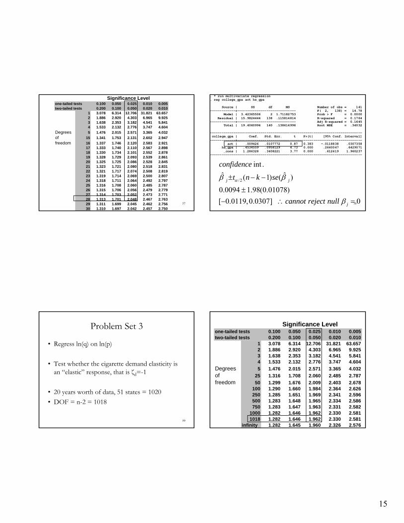
. * run multivariate regression

. reg college_gpa act hs_gpa Source | SS df MS Number of obs = 141 -------------+------------------------------ F( 2, 138) = 14.78 Model | 3.42365506 2 1.71182753 Prob > F = 0.0000 Residual | 15.9824444 138 .115814814 R-squared = 0.1764 -------------+------------------------------ Adj R-squared = 0.1645 Total | 19.4060994 140 .138614996 Root MSE = .34032 ------------------------------------------------------------------------------ college_gpa | Coef. Std. Err. t P>|t| [95% Conf. Interval] -------------+---------------------------------------------------------------- act | .009426 .0107772 0.87 0.383 -.0118838 .0307358 hs_gpa | .4534559 .0958129 4.73 0.000 .2640047 .6429071 _cons | 1.286328 .3408221 3.77 0.000 .612419 1.960237 ------------------------------------------------------------------------------

/2

int .

ˆ ˆ( 1) ( )

0.0094 1.98(0.01078)

[ 0.0119,0.0307] 0

j j

j

confidence

t n k se

cannot reject null

59

Problem Set 3

• Regress ln(q) on ln(p)

• Test whether the cigarette demand elasticity is an “elastic” response, that is ζd=-1

• 20 years worth of data, 51 states = 1020

• DOF = n-2 = 1018

60

Significance Levelone-tailed tests 0.100 0.050 0.025 0.010 0.005two-tailed tests 0.200 0.100 0.050 0.020 0.010 1 3.078 6.314 12.706 31.821 63.657

2 1.886 2.920 4.303 6.965 9.9253 1.638 2.353 3.182 4.541 5.8414 1.533 2.132 2.776 3.747 4.604

Degrees 5 1.476 2.015 2.571 3.365 4.032

of 25 1.316 1.708 2.060 2.485 2.787

freedom 50 1.299 1.676 2.009 2.403 2.678100 1.290 1.660 1.984 2.364 2.626250 1.285 1.651 1.969 2.341 2.596500 1.283 1.648 1.965 2.334 2.586750 1.283 1.647 1.963 2.331 2.582

1000 1.282 1.646 1.962 2.330 2.5811018 1.282 1.646 1.962 2.330 2.581

infinity 1.282 1.645 1.960 2.326 2.576

16

61

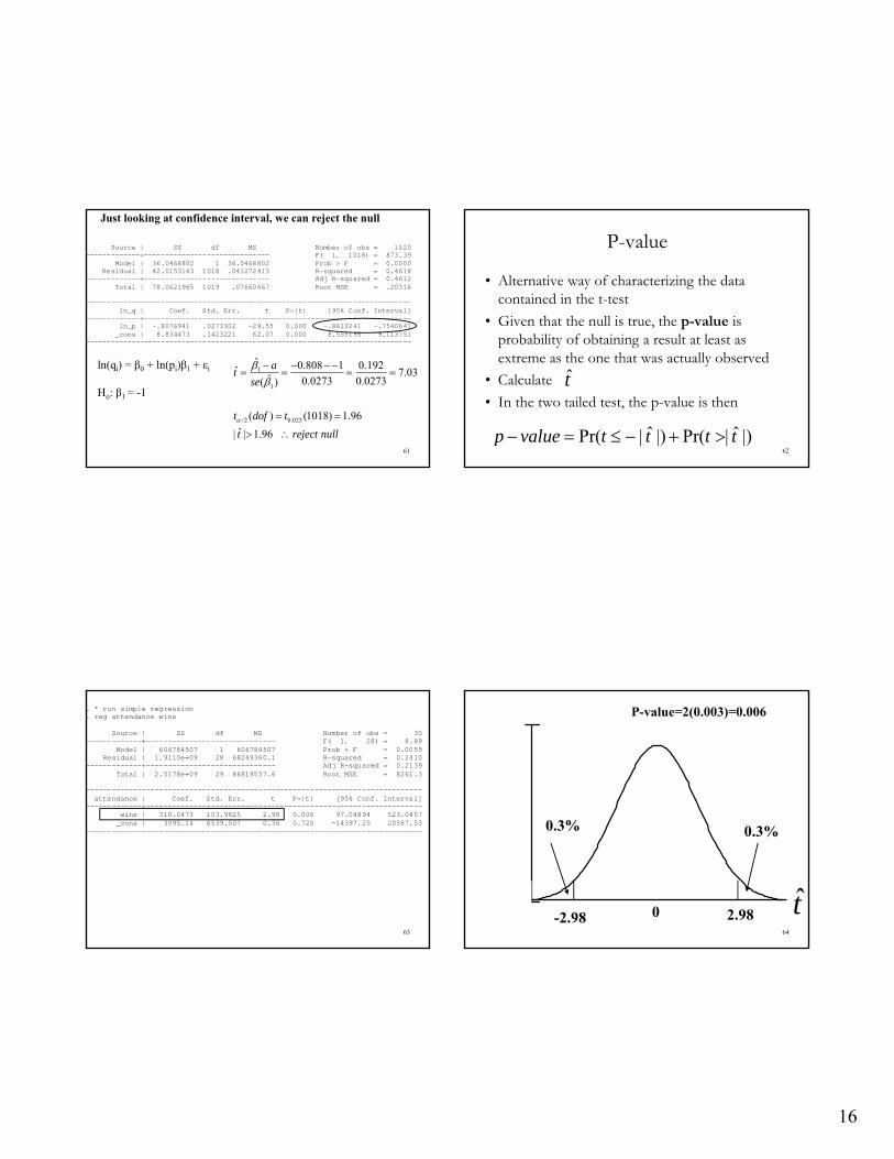
Source | SS df MS Number of obs = 1020 -------------+------------------------------ F( 1, 1018) = 873.39 Model | 36.0468802 1 36.0468802 Prob > F = 0.0000 Residual | 42.0153163 1018 .041272413 R-squared = 0.4618 -------------+------------------------------ Adj R-squared = 0.4612 Total | 78.0621965 1019 .07660667 Root MSE = .20316 ------------------------------------------------------------------------------ ln_q | Coef. Std. Err. t P>|t| [95% Conf. Interval] -------------+---------------------------------------------------------------- ln_p | -.8076941 .0273302 -29.55 0.000 -.8613241 -.7540641 _cons | 8.834473 .1423221 62.07 0.000 8.555195 9.113751 ------------------------------------------------------------------------------

ln(qi) = β0 + ln(pi)β1 + εi

Ho: β1 = -1

1

1

/2 0.025

ˆ 0.808 1 0.192ˆ 7.03ˆ 0.0273 0.0273( )

( ) (1018) 1.96

ˆ| | 1.96

at

se

t dof t

t reject null

Just looking at confidence interval, we can reject the null

62

P-value

• Alternative way of characterizing the data contained in the t-test

• Given that the null is true, the p-value is probability of obtaining a result at least as extreme as the one that was actually observed

• Calculate

• In the two tailed test, the p-value is thent̂

ˆ ˆPr( | |) Pr( | |)p value t t t t

63

. * run simple regression

. reg attendance wins Source | SS df MS Number of obs = 30 -------------+------------------------------ F( 1, 28) = 8.89 Model | 606784507 1 606784507 Prob > F = 0.0059 Residual | 1.9110e+09 28 68249360.1 R-squared = 0.2410 -------------+------------------------------ Adj R-squared = 0.2139 Total | 2.5178e+09 29 86819537.6 Root MSE = 8261.3 ------------------------------------------------------------------------------ attendance | Coef. Std. Err. t P>|t| [95% Conf. Interval] -------------+---------------------------------------------------------------- wins | 310.0473 103.9825 2.98 0.006 97.04894 523.0457 _cons | 3095.14 8539.507 0.36 0.720 -14397.25 20587.53 ------------------------------------------------------------------------------

64

0

0.45

t̂0

0.3% 0.3%

-2.98 2.98

P-value=2(0.003)=0.006

17

65

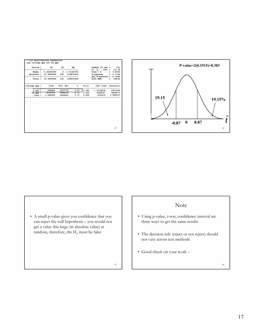
. * run multivariate regression

. reg college_gpa act hs_gpa Source | SS df MS Number of obs = 141 -------------+------------------------------ F( 2, 138) = 14.78 Model | 3.42365506 2 1.71182753 Prob > F = 0.0000 Residual | 15.9824444 138 .115814814 R-squared = 0.1764 -------------+------------------------------ Adj R-squared = 0.1645 Total | 19.4060994 140 .138614996 Root MSE = .34032 ------------------------------------------------------------------------------ college_gpa | Coef. Std. Err. t P>|t| [95% Conf. Interval] -------------+---------------------------------------------------------------- act | .009426 .0107772 0.87 0.383 -.0118838 .0307358 hs_gpa | .4534559 .0958129 4.73 0.000 .2640047 .6429071 _cons | 1.286328 .3408221 3.77 0.000 .612419 1.960237 ------------------------------------------------------------------------------

66

0

0.45

t̂0

19.15 19.15%

-0.87 0.87

P-value=2(0.1915)=0.383

67

• A small p-value gives you confidence that you can reject the null hypothesis – you would not get a value this large (in absolute value) at random, therefore, the Ho must be false

Note

• Using p-value, t-test, confidence interval are three ways to get the same results

• The decision rule (reject or not reject) should not vary across test methods

• Good check on your work --

68

18

69

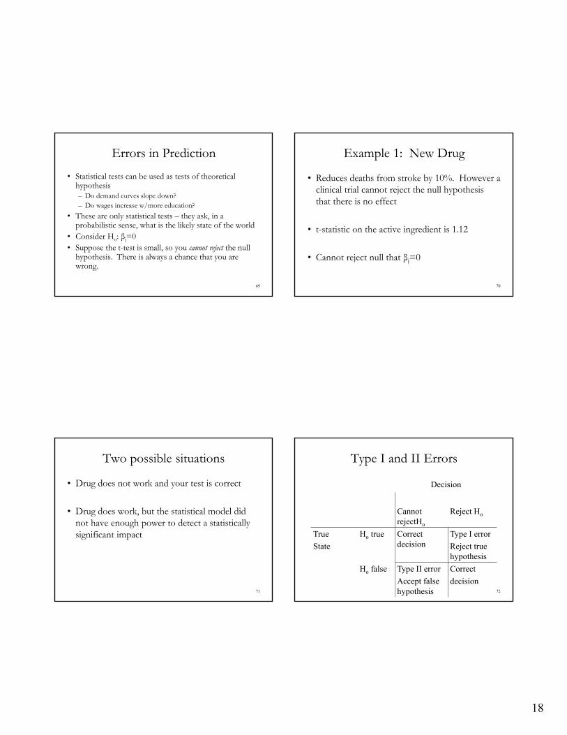
Errors in Prediction

• Statistical tests can be used as tests of theoretical hypothesis– Do demand curves slope down?– Do wages increase w/more education?

• These are only statistical tests – they ask, in a probabilistic sense, what is the likely state of the world

• Consider Ho: βj=0• Suppose the t-test is small, so you cannot reject the null

hypothesis. There is always a chance that you are wrong.

70

Example 1: New Drug

• Reduces deaths from stroke by 10%. However a clinical trial cannot reject the null hypothesis that there is no effect

• t-statistic on the active ingredient is 1.12

• Cannot reject null that βj=0

71

Two possible situations

• Drug does not work and your test is correct

• Drug does work, but the statistical model did not have enough power to detect a statistically significant impact

72

Type I and II Errors

Decision

Cannot rejectHo

Reject Ho

True

State

Ho true Correct decision

Type I error

Reject true hypothesis

Ho false Type II error

Accept false hypothesis

Correct

decision

19

73

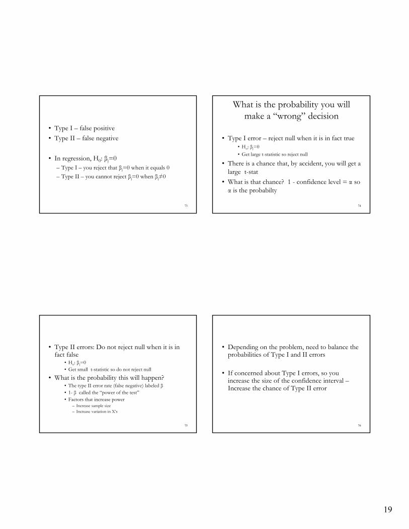
• Type I – false positive

• Type II – false negative

• In regression, H0: βj=0– Type I – you reject that βj=0 when it equals 0

– Type II – you cannot reject βj=0 when βj≠0

74

What is the probability you will make a “wrong” decision

• Type I error – reject null when it is in fact true• Ho: βj=0

• Get large t-statistic so reject null

• There is a chance that, by accident, you will get a large t-stat

• What is that chance? 1 - confidence level = α so α is the probabilty

75

• Type II errors: Do not reject null when it is in fact false

• Ho: βj=0• Get small t-statistic so do not reject null

• What is the probability this will happen? • The type II error rate (false negative) labeled β• 1- β called the “power of the test”• Factors that increase power

– Increase sample size– Increase variation in X’s

76

• Depending on the problem, need to balance the probabilities of Type I and II errors

• If concerned about Type I errors, so you increase the size of the confidence interval –Increase the chance of Type II error

20

77

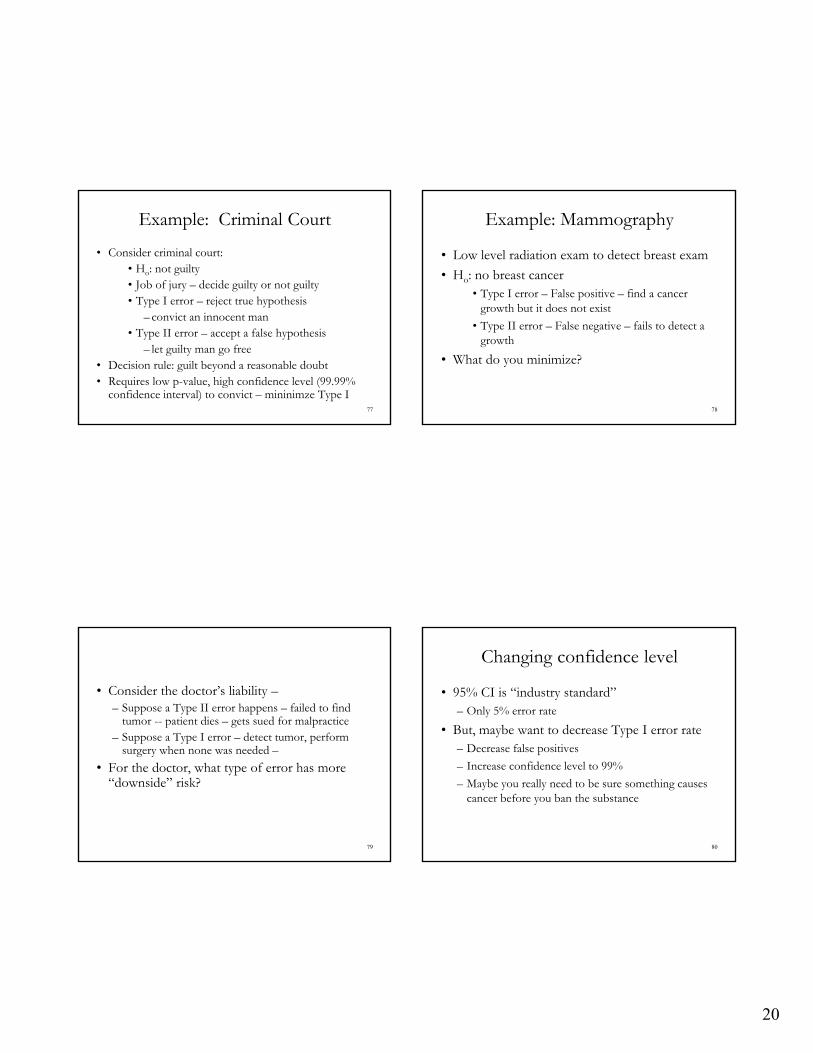
Example: Criminal Court

• Consider criminal court:• Ho: not guilty• Job of jury – decide guilty or not guilty• Type I error – reject true hypothesis

– convict an innocent man• Type II error – accept a false hypothesis

– let guilty man go free• Decision rule: guilt beyond a reasonable doubt• Requires low p-value, high confidence level (99.99%

confidence interval) to convict – mininimze Type I78

Example: Mammography

• Low level radiation exam to detect breast exam

• Ho: no breast cancer• Type I error – False positive – find a cancer

growth but it does not exist

• Type II error – False negative – fails to detect a growth

• What do you minimize?

79

• Consider the doctor’s liability –– Suppose a Type II error happens – failed to find

tumor -- patient dies – gets sued for malpractice– Suppose a Type I error – detect tumor, perform

surgery when none was needed –

• For the doctor, what type of error has more “downside” risk?

80

Changing confidence level

• 95% CI is “industry standard”– Only 5% error rate

• But, maybe want to decrease Type I error rate– Decrease false positives

– Increase confidence level to 99%

– Maybe you really need to be sure something causes cancer before you ban the substance

21

81

• In contrast, you might want to decrease chance of Type II error– Reduce the size of the confidence interval

– Maybe do not require as definitive evidence before you let on the market a new drug to treat in uncurable disease

82

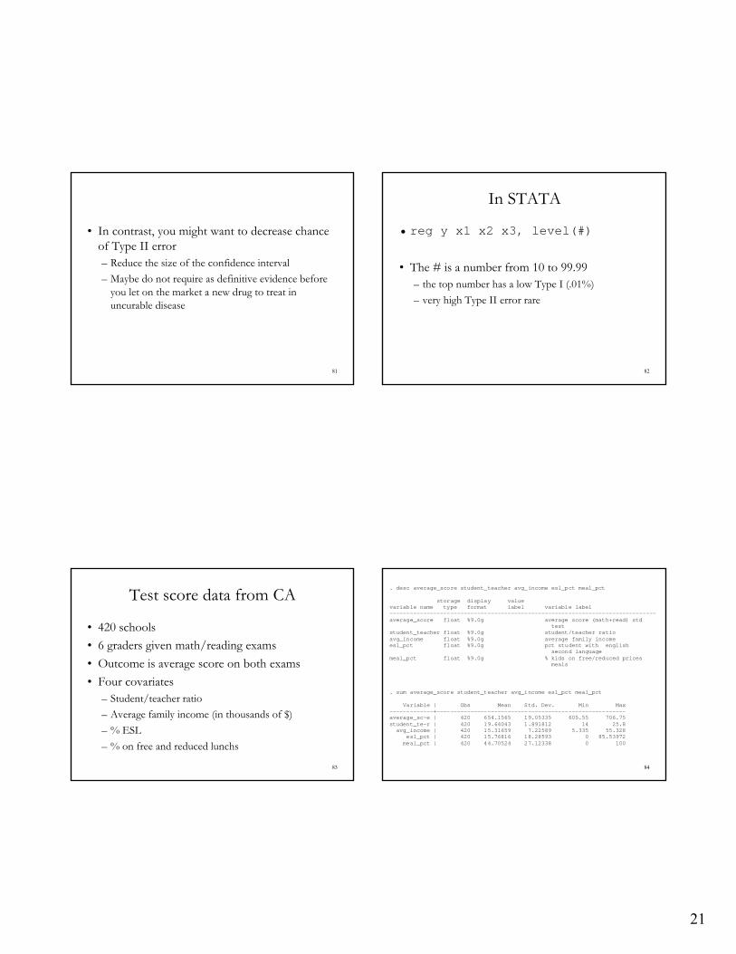
In STATA

• reg y x1 x2 x3, level(#)

• The # is a number from 10 to 99.99– the top number has a low Type I (.01%)

– very high Type II error rare

83

Test score data from CA

• 420 schools

• 6 graders given math/reading exams

• Outcome is average score on both exams

• Four covariates– Student/teacher ratio

– Average family income (in thousands of $)

– % ESL

– % on free and reduced lunchs

84

. desc average_score student_teacher avg_income esl_pct meal_pct storage display value variable name type format label variable label -------------------------------------------------------------------------------average_score float %9.0g average score (math+read) std test student_teacher float %9.0g student/teacher ratio avg_income float %9.0g average family income esl_pct float %9.0g pct student with english second language meal_pct float %9.0g % kids on free/reduced prices meals

. sum average_score student_teacher avg_income esl_pct meal_pct Variable | Obs Mean Std. Dev. Min Max -------------+-------------------------------------------------------- average_sc~e | 420 654.1565 19.05335 605.55 706.75 student_te~r | 420 19.64043 1.891812 14 25.8 avg_income | 420 15.31659 7.22589 5.335 55.328 esl_pct | 420 15.76816 18.28593 0 85.53972 meal_pct | 420 44.70524 27.12338 0 100

22

85

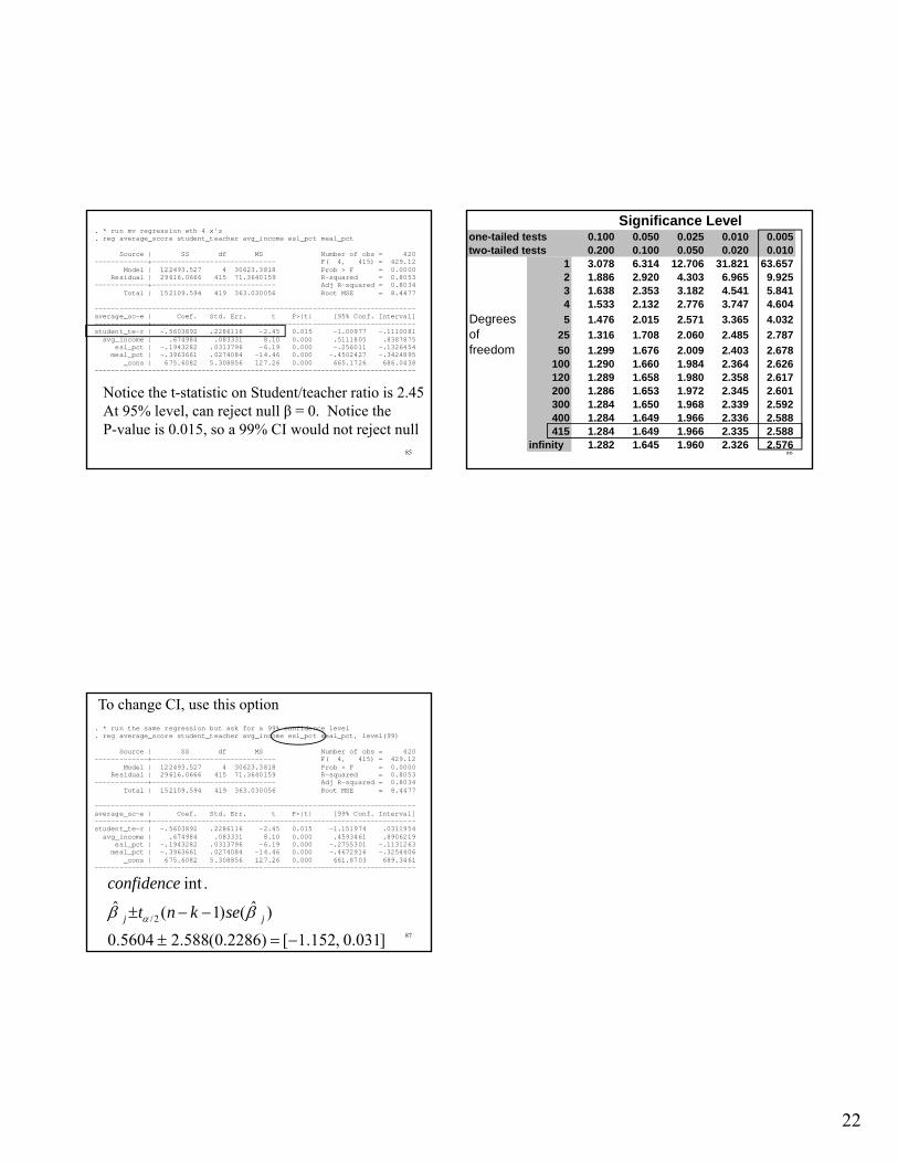
. * run mv regression wth 4 x's

. reg average_score student_teacher avg_income esl_pct meal_pct Source | SS df MS Number of obs = 420 -------------+------------------------------ F( 4, 415) = 429.12 Model | 122493.527 4 30623.3818 Prob > F = 0.0000 Residual | 29616.0666 415 71.3640159 R-squared = 0.8053 -------------+------------------------------ Adj R-squared = 0.8034 Total | 152109.594 419 363.030056 Root MSE = 8.4477 ------------------------------------------------------------------------------ average_sc~e | Coef. Std. Err. t P>|t| [95% Conf. Interval] -------------+---------------------------------------------------------------- student_te~r | -.5603892 .2286116 -2.45 0.015 -1.00977 -.1110081 avg_income | .674984 .083331 8.10 0.000 .5111805 .8387875 esl_pct | -.1943282 .0313796 -6.19 0.000 -.256011 -.1326454 meal_pct | -.3963661 .0274084 -14.46 0.000 -.4502427 -.3424895 _cons | 675.6082 5.308856 127.26 0.000 665.1726 686.0438 ------------------------------------------------------------------------------

Notice the t-statistic on Student/teacher ratio is 2.45At 95% level, can reject null β = 0. Notice the P-value is 0.015, so a 99% CI would not reject null

86

Significance Levelone-tailed tests 0.100 0.050 0.025 0.010 0.005two-tailed tests 0.200 0.100 0.050 0.020 0.010 1 3.078 6.314 12.706 31.821 63.657

2 1.886 2.920 4.303 6.965 9.9253 1.638 2.353 3.182 4.541 5.8414 1.533 2.132 2.776 3.747 4.604

Degrees 5 1.476 2.015 2.571 3.365 4.032

of 25 1.316 1.708 2.060 2.485 2.787

freedom 50 1.299 1.676 2.009 2.403 2.678100 1.290 1.660 1.984 2.364 2.626120 1.289 1.658 1.980 2.358 2.617200 1.286 1.653 1.972 2.345 2.601300 1.284 1.650 1.968 2.339 2.592400 1.284 1.649 1.966 2.336 2.588415 1.284 1.649 1.966 2.335 2.588

infinity 1.282 1.645 1.960 2.326 2.576

87

. * run the same regression but ask for a 99% confidence level

. reg average_score student_teacher avg_income esl_pct meal_pct, level(99) Source | SS df MS Number of obs = 420 -------------+------------------------------ F( 4, 415) = 429.12 Model | 122493.527 4 30623.3818 Prob > F = 0.0000 Residual | 29616.0666 415 71.3640159 R-squared = 0.8053 -------------+------------------------------ Adj R-squared = 0.8034 Total | 152109.594 419 363.030056 Root MSE = 8.4477 ------------------------------------------------------------------------------ average_sc~e | Coef. Std. Err. t P>|t| [99% Conf. Interval] -------------+---------------------------------------------------------------- student_te~r | -.5603892 .2286116 -2.45 0.015 -1.151974 .0311954 avg_income | .674984 .083331 8.10 0.000 .4593461 .8906219 esl_pct | -.1943282 .0313796 -6.19 0.000 -.2755301 -.1131263 meal_pct | -.3963661 .0274084 -14.46 0.000 -.4672916 -.3254406 _cons | 675.6082 5.308856 127.26 0.000 661.8703 689.3461 ------------------------------------------------------------------------------

To change CI, use this option

/2

int .

ˆ ˆ( 1) ( )

0.5604 2.588(0.2286) [ 1.152, 0.031]

j j

confidence

t n k se