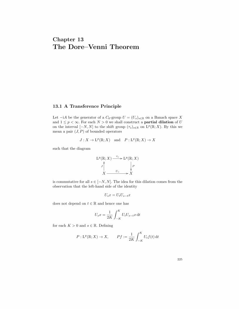
Chapter 13

The Dore–Venni Theorem

13.1 A Transference Principle

Let −iA be the generator of a C0-group U = (Us)s∈R on a Banach space Xand 1 ≤ p <∞. For each N > 0 we shall construct a partial dilation of Uon the interval [−N,N ] to the shift group (τs)s∈R on Lp(R;X). By this wemean a pair (J, P ) of bounded operators

J : X → Lp(R;X) and P : Lp(R;X)→ X

such that the diagram

Lp(R;X)τs // Lp(R;X)

P

X

J

OO

Us // X

is commutative for all s ∈ [−N,N ]. The idea for this dilation comes from theobservation that the left-hand side of the identity

Usx = UtUs−tx

does not depend on t ∈ R and hence one has

Usx =1

2K

∫ K

−KUtUs−txdt

for each K > 0 and s ∈ R. Defining

P : Lp(R;X)→ X, Pf :=1

2K

∫ K

−KUtf(t) dt

225

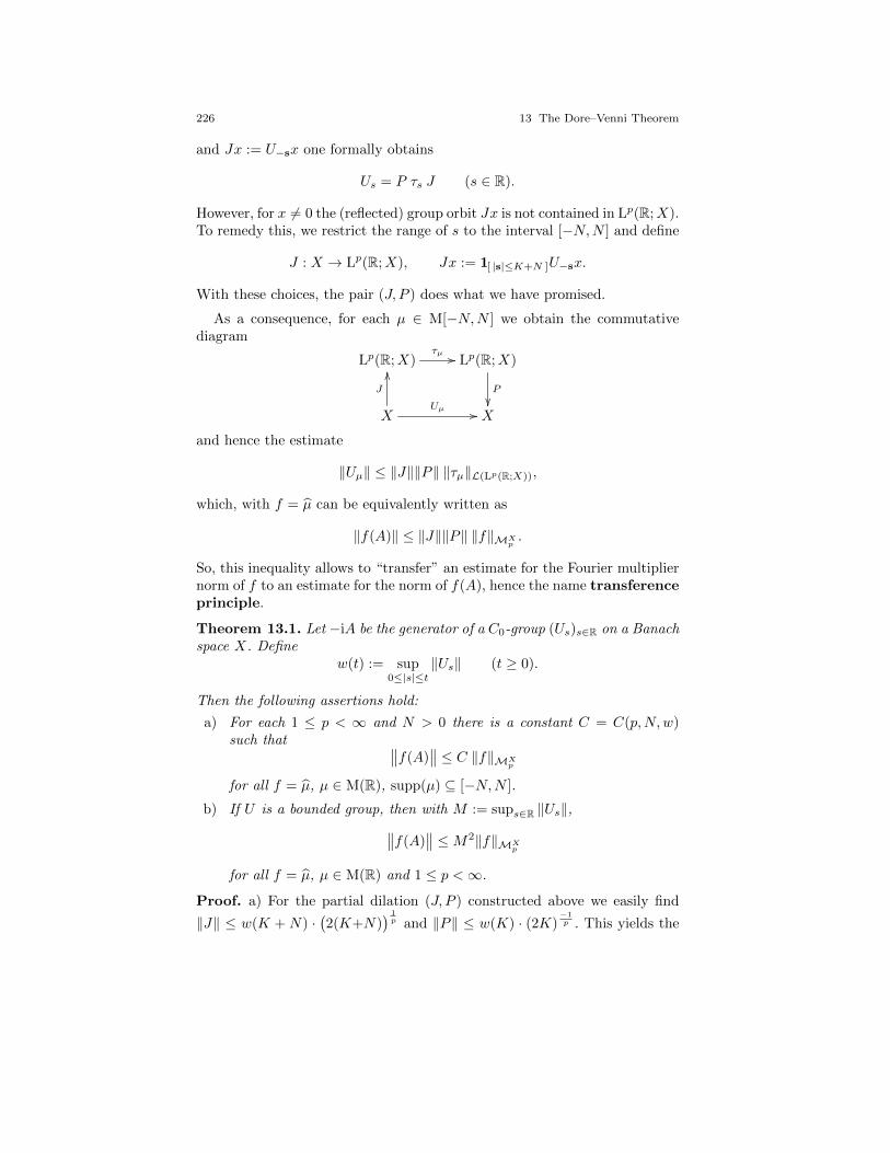
226 13 The Dore–Venni Theorem

and Jx := U−sx one formally obtains

Us = P τs J (s ∈ R).

However, for x 6= 0 the (reflected) group orbit Jx is not contained in Lp(R;X).To remedy this, we restrict the range of s to the interval [−N,N ] and define

J : X → Lp(R;X), Jx := 1[ |s|≤K+N ]U−sx.

With these choices, the pair (J, P ) does what we have promised.

As a consequence, for each µ ∈ M[−N,N ] we obtain the commutativediagram

Lp(R;X)τµ // Lp(R;X)

P

X

J

OO

Uµ // X

and hence the estimate

‖Uµ‖ ≤ ‖J‖‖P‖ ‖τµ‖L(Lp(R;X)),

which, with f = µ can be equivalently written as

‖f(A)‖ ≤ ‖J‖‖P‖ ‖f‖MXp.

So, this inequality allows to “transfer” an estimate for the Fourier multipliernorm of f to an estimate for the norm of f(A), hence the name transferenceprinciple.

Theorem 13.1. Let −iA be the generator of a C0-group (Us)s∈R on a Banachspace X. Define

w(t) := sup0≤|s|≤t

‖Us‖ (t ≥ 0).

Then the following assertions hold:

a) For each 1 ≤ p < ∞ and N > 0 there is a constant C = C(p,N,w)such that ∥∥f(A)

∥∥ ≤ C ‖f‖MXp

for all f = µ, µ ∈ M(R), supp(µ) ⊆ [−N,N ].

b) If U is a bounded group, then with M := sups∈R ‖Us‖,∥∥f(A)∥∥ ≤M2‖f‖MX

p

for all f = µ, µ ∈ M(R) and 1 ≤ p <∞.

Proof. a) For the partial dilation (J, P ) constructed above we easily find

‖J‖ ≤ w(K + N) ·(2(K+N)

) 1p and ‖P‖ ≤ w(K) · (2K)

−1p . This yields the

13.1 A Transference Principle 227

claim of a) with

C(p,N,w) := infK>0

w(K+N) w(K)(

1 +N

K

) 1p

. (13.1)

b) If ‖Us‖ ≤M for all s ∈ R then for the constant from a) we obtain

C ≤ infK>0

M2(

1 +N

K

) 1p

= M2.

Hence, in this case the dependence on N > 0 has vanished and since Mc(R)is dense in M(R), the claim of b) follows.

Remark 13.2. Part b) of Theorem 13.1 is the special case G = R of a resultby Berkson–Gillespie-Muhly [3] for general locally compact amenable groupsG. That theorem, in turn, is the vector-valued version of its scalar analoguedue to Coifman and Weiss from [6]. Our proof is the original one, suitablyadapted.

Lemma 13.3. Let 1 ≤ p <∞ and let the Banach space X 6= 0 be a closedsubspace of a space Lp(Ω) for some measure space Ω. Then

‖µ‖Mp= ‖µ‖MX

p.

for each µ ∈ M(Rd).

Proof. The implication ‖µ‖Mp ≤ ‖µ‖MXp

is Theorem A.55.b) and holdsfor any Banach space X. For the converse, note that one has an isometricisomorphism

ι : Lp(Rd; Lp(Ω))→ Lp(Ω; Lp(Rd))

that commutes with the translation group and hence with the convolutionoperator τµ. By this is meant that

ιτµf = τµ (ιf)(f ∈ Lp(Rd; Lp(Ω))

).

Since ι is isometric, it easily follows that

‖τµf‖Lp(Rd;X) ≤ ‖µ‖Mp ‖f‖Lp(Rd;X)

for each f ∈ Lp(Rd;X), i.e., the claim.

Remark 13.4. With more effort one can even show MXp (Rd) = Mp(Rd)

isometrically if X is a closed subspace of an Lp-space, but we shall not needthis in the following.

228 13 The Dore–Venni Theorem

13.2 The Hilbert Transform and UMD Spaces

One of the simplest non-trivial candidates for an Lp(R;X)-Fourier multiplieris the function

h := −i sgn t.

Since h′ = 0 on R \ 0, h is a Mikhlin function on R \ 0, and hence, bythe Mikhlin multiplier theorem, H := Th is a bounded operator on Lp(R) for1 < p <∞. It is called the Hilbert transform1

A Banach space X is called an HTp space if h ∈MXp (R). In this case,

CHTp(X) := ‖h‖MXp

is called theHTp-constant of X. Recall that, unless X = 0, any L1-Fouriermultiplier is the Fourier transform of a measure and hence continuous. SoX 6= 0 can be an HTp space only if 1 < p <∞. Define

hε,T := F(1[ ε≤|s|≤T ]

π s

)=

2

πi

∫ T

ε

sin(st)

sds (0 < ε ≤ T <∞).

The following is an important characterization of the HTp-property. (Weuse the convention that a Fourier multiplier norm ‖m‖MX

pequals +∞ if

m /∈MXp (R).)

Theorem 13.5. There is a constant C ≥ 1 such that for every Banach spaceX and every 1 < p <∞

‖h‖MXp≤ sup

0<ε≤1‖hε,1‖MX

p= sup

0<ε≤T<∞‖hε,T ‖MX

p≤ C ‖h‖MX

p.

In particular, the following assertions are equivalent:

(i) X is an HTp space;

(ii) sup0<ε≤1 ‖hε,1‖MXp<∞;

(iii) sup0<ε≤T<∞ ‖hε,T ‖MXp<∞.

Proof. Trivially, the inequality sup0<ε≤1 ‖hε,1‖MXp≤ sup0<ε≤T<∞ ‖hε,T ‖MX

p

holds. For the converse inequality, note that

hε,T =2

πi

∫ T

ε

sin(ts)

sds =

2

πi

∫ 1

ε/T

sin(tTs)

sds = h ε

T ,1(T t).

Hence, ‖hε,T ‖MXp

= ‖h εT ,1‖MX

pby Theorem A.55.h) (with A being multipli-

cation by T ).

1 Actually, the boundedness of the Hilbert transform is one of the “first” results on the

theory of singular integrals and multipliers, and does not need the full force of the Mikhlin

multiplier theorem. See [9, Thm.4.1.7].

13.2 The Hilbert Transform and UMD Spaces 229

Define mn := h 1n ,n

. Then mn → h pointwise on R \ 0. Hence

π‖h‖MXp≤ sup

n‖mn‖MX

p

by Theorem A.55.g).

For the final inequality we write

πi

2hε,T =

∫ T

ε

sin(ts)

sds = sgn(t)

∫ T

ε

sin(|t| s)s

ds = sgn(t)(f(εt)− f(T t)

)where

f(t) :=

∫ ∞|t|

sin s

sds (t ∈ R).

By Exercise 13.3, f ∈ F(L1(R)) ⊆ FS(R). It follows that the functions f(εt)−f(T t), 0 < ε ≤ T <∞, are uniformly bounded in MX

p (R), by 2‖f‖FS. Since

MXp (R) is a Banach algebra (Theorem 12.1, Theorem A.55.f)), we obtain

sup0<ε≤T<∞

‖hε,T ‖MXp≤(

4/π‖f‖FS

)‖h‖MX

p

as claimed.

Corollary 13.6. Let 1 < p <∞.

a) Each Hilbert space is an HT2 space.

b) Each closed subspace of an HTp space is an HTp space.

c) Lp(Ω) is an HTp space for any measure space Ω. More generally, if Xis an HTp space, then so is Lp(Ω;X).

Proof. The first part of c) follows from Lemma 13.3. For the second partone needs a vector-valued version Lemma 13.3, but we skip the proof.

Remark 13.7. It follows from a result of Benedek, Calderon and Panzonefrom [2] that if a Banach space X is an HTp space for one p ∈ (1,∞) thenit is an HTp space for all p ∈ (1,∞). Hence, one can drop the reference to pand call them simply HT spaces.

By results of Burkholder [5] and Bourgain [4] the class of HT spacescoincides with the class of the so-called UMD spaces. These are definedvia the requirement that certain vector-valued martingale differences areunconditional in Lp. We do not need this description and hence refer to [12]for a thorough treatment. However, we shall adopt the name “UMD spaces”in the following.

One can show that UMD spaces are reflexive, see [12, Thm.4.3.3].

230 13 The Dore–Venni Theorem

13.3 Singular Integrals for Groups and Monniaux’sTheorem

We now combine the transference principle and Theorem 13.5.

Theorem 13.8. Let −iA be the generator of a C0-group U = (Us)s∈R on aUMD space X. Then the following assertions hold:

a) The principle value integral

HU1 x :=1

πp.v.

∫ 1

−1

Usx

sds := lim

ε0

1

π

∫ε≤|s|≤1

Usx

sds (13.2)

converges for all x ∈ X.

b) If U is bounded and A is injective, the principle value integral

HUx :=1

πp.v.

∫ ∞−∞

Usx

sds := lim

ε↓0,T↑∞

1

π

∫ε≤|s|≤T

Usx

sds (13.3)

converges for all x ∈ X.

Proof. a) Note that, for any x ∈ X and 0 < ε ≤ 1,∫ε≤|s|≤1

Usx

sds =

∫ε≤|s|≤1

Usx− xs

ds.

This shows that the principle value integral (13.2) exists for all x ∈ dom(A).Since dom(A) is dense, it suffices to show that the family of operators

Sε :=

∫ε≤|s|≤1

Uss

ds (0 < ε ≤ 1)

is uniformly bounded. Since X is an HTp space for any 1 < p <∞, Theorem13.5 together with the transference principle (Theorem 13.1) yields the claim.

b) As before, the principal value integral (13.2) converges as ε 0 for x ∈dom(A). If x = (−iA)y ∈ ran(A), however, integration by parts yields∫

1≤|s|≤T

Usx

sds =

∫1≤|s|≤T

Us(−iAy)

sds

=UT y + U−T y

T− (U1y + U−1y) +

∫1≤|s|≤T

Usy

s2ds

and this converges as T ∞. Hence, the principal value integral (13.3)converges for x ∈ dom(A) ∩ ran(A).

By Remark 13.7, X is reflexive. Since −iA is a densely defined injectivesectorial operator on X, dom(A) ∩ ran(A) is dense in X. Hence, as before itsuffices to show that the family of operators

13.3 Singular Integrals for Groups and Monniaux’s Theorem 231

Sε,T :=

∫ε≤|s|≤T

Uss

ds (0 < ε ≤ T <∞)

is uniformly bounded. Again, Theorem 13.5 combined with the transferenceprinciple (Theorem 13.1) yields the claim.

Remark 13.9. The proof of Theorem 13.8 actually yields more than what isstated in the theorem. Indeed, a re-examination of the proof and employing(13.1) yields

‖HU1 ‖L(X) ≤ C 21p(

sup|s|≤2

‖Us‖)2CHTp(X)

for the (universal) constant C from Theorem 13.5. A similar remark is validfor the norm of HU in case of a bounded group.

Monniaux’s Theorem

Theorem 13.8 can be reformulated in functional calculus terms. Namely, forscalars z ∈ C we have

h0,1(z) :=1

πp.v.

∫ 1

−1

e−isz

sds =

2

πi

∫ 1

0

sin zs

sds.

By Exercise 13.4, h0,1 ∈ H∞(Stω) for each ω > 0 satisfying

lim|Im z|≤ω,Re z→±∞

h0,1(z) = ∓i.

Moreover,

h0,1(z) =2

πi

∫ z

0

sin s

sds,

where the right hand side is to be understood as a complex line integralover the straight line segment from 0 to z. In other words, h0,1 is the uniqueprimitive of the function 2 sin z/πiz which vanishes at z = 0.

So, part a) of Theorem 13.8 essentially says that h0,1(A) ∈ L(X) whenever−iA generates a C0-group on a UMD space.

Theorem 13.10 (Monniaux). Let −iA be the generator of a C0-group(Us)s∈R on a UMD space X with θ(U) < π. Then eA is a sectorial oper-ator. In particular, A is the logarithm of a sectorial operator.

Proof. By Remark 10.6, the second assertion follows from the first. The first,in turn, amounts to proving that( t

t+ ez

)(A), t > 0

is a bounded family of bounded operators. To achieve this, we make use ofthe representation

232 13 The Dore–Venni Theorem

t

t+ ez=

1

2+

1

2ip.v.

∫Rtise−isz ds

sinh(πs)(13.4)

which holds for all z ∈ Stπ and t > 0. (Actually, by replacing z by z + log twe see that it suffices to establish the formula for t = 1. A proof is left asExercise 13.9.)

Observe that the integral (13.4) is singular only at 0 since |Im z| < π. Taking(13.4) for granted, we can write

(2i)t

t+ ez= i +

∫|s|≥1

tise−isz ds

sinh(πs)+

∫ 1

−1

tise−isz( 1

sinh(πs)− 1

πs

)ds

+1

πp.v.

∫ 1

−1

tise−isz

sds

=(µ+ h0,1

)(z − log t)

for some µ ∈ Mω(R). By Theorem 13.8 inserting A we find that t(t+eA)−1 isa bounded operator. Since for t > 0 all the groups tisUs have the same growthbehaviour, it follows from Remark 13.9 that supt>0 ‖t(t+ eA)−1‖ <∞.

13.4 The Maximal Regularity Problem

Let A be a densely defined sectorial operator of angle ωse(A) < π/2 on aBanach space X. (For example, A could be a strongly elliptic operator onX = Lp(Rd) as treated in Chapter 12.) As such, −A generates a boundedholomorphic C0-semigroup T = (Tt)t≥0 on X (Chapter 9).

Given an initial value x ∈ X, the trajectory u(t) := Ttx is a so-called“mild” solution to the homogeneous Cauchy problem

u′(t) +Au(t) = 0 (t > 0),

u(0) = x.

For example, if A = −∆ on Lp(Rd) then (Tt)t≥0 is the heat semigroup andu solves the homogeneous parabolic equation

d

dtu = ∆u.

Using the semigroup T one can also construct “mild” solutions to the (finitetime) inhomogeneous Cauchy problem

u′(t) +Au(t) = f(t) (0 < t < 1),

u(0) = x,(13.5)

13.4 The Maximal Regularity Problem 233

where f ∈ L1((0, 1);X), namely

u(t) = Ttx+

∫ t

0

Tt−sf(s) ds (0 ≤ t ≤ 1).

In the following we shall restrict ourselves to the case x = 0, which amountsto

u(t) = (Sf)(t) :=

∫ t

0

Tt−sf(s) ds (0 ≤ t ≤ 1). (13.6)

(See Exercise 13.5 for a proof that u is a “mild” solution of (13.5) with x = 0.)

Given p ∈ (1,∞) one says that A has maximal Lp-regularity if thesolution u = Sf given by (13.6) satisfies

f ∈ Lp((0, 1);X) ⇒ u′, Au ∈ Lp((0, 1);X). (13.7)

Here, Au ∈ Lp((0, 1);X) means that u ∈ Lp((0, 1); dom(A)) and u′ ∈Lp((0, 1);X) means that there is v ∈ Lp((0, 1);X) with

u(t) =

∫ t

0

v(s) ds (0 ≤ t ≤ 1).

The terminology stems from the fact that both summands on the left-handside of the equation

u′ +Au = f

should have the maximal “amount of regularity” that one can reasonablyexpect, given that the right-hand side f is in Lp.

The maximal regularity problem consists in deciding whether a givenoperator has maximal Lp-regularity or not. One can show that if A has max-imal Lp-regularity for one 1 < p < ∞, then this is true for all such p. Asa result, one often drops the reference to p and only speaks of “maximalregularity”.

Remark 13.11. One may wonder why we have confined ourselves to genera-tors of holomorphic semigroups. Indeed, all the notions and definitions so farare meaningful for general C0-semigroups. However, Dore has shown in [7]that the holomorphy of the semigroup is necessary for maximal Lp-regularity.

Operator-Theoretic Reformulation

In the following we briefly sketch how the maximal regularity problem can bereformulated in purely operator-theoretic terms. To this aim we fix p ∈ (1,∞)and pass to the new Banach space

Xp := Lp((0, 1);X).

234 13 The Dore–Venni Theorem

On Xp we consider the operator A given by

dom(A) := Lp((0, 1); dom(A)), (Au)(t) := A(u(t)) (t ∈ (0, 1)).

It is easy to see that A inherits from A many of its properties (Exercise 13.6).For example, A is a densely defined sectorial operator of angle ωse(A) =ωse(A).

We also consider the operator B := V −1, where V is the Volterra operatoron X defined by

(V u)(t) :=

∫ t

0

u(s) ds (0 ≤ t ≤ 1).

As in the scalar case (Exercise 6.6) one can prove that −B is the generatorof the right shift semigroup (τs)s≥0. As such, B is a densely defined andinvertible sectorial operator of angle π/2. Its domain is

dom(B) = ran(V ) = u ∈W1,p((0, 1);X) | u(0) = 0,

but we shall not need the second identity.

Using the operators A and B on X , one can reformulate the maximalregularity property of A as follows.

Lemma 13.12. Let A be a sectorial operator of angle ωse(A) < π/2 on aBanach space X, and let the operators A and B on Xp = Lp((0, 1);X) bedefined as above. Then the following assertions are equivalent:

(i) A has maximal Lp-regularity;

(ii) There is a constant K ≥ 0 such that

‖Au‖Xp + ‖Bu‖Xp ≤ K‖Au+ Bu‖Xp

for all u ∈ dom(A) ∩ dom(B);

(iii) The operator A+ B defined on dom(A) ∩ dom(B) is closed.

Proof. By definition of A and B, (i) is equivalent to the assertion: For eachf ∈ Xp one has Sf ∈ dom(A)∩dom(B). Since A and B are closed operators,dom(A) ∩ dom(B) is a Banach space with respect to the norm

|||u ||| := ‖u‖Xp + ‖Au‖Xp + ‖Bu‖Xp .

(ii)⇒ (i): It follows from (ii) that

|||u ||| ≤ ‖u‖Xp +K‖Au+ Bu‖Xp ≤ (K + 1)(‖Au+ Bu‖Xp + ‖u‖Xp)

for all u ∈ dom(A)∩dom(B). Now, given f ∈ C([0, 1]; dom(A)), let u := Sf bedefined by (13.6). Then u ∈ C1([0, 1];X)∩C([0, 1]; dom(A)) and Au+u′ = f

13.4 The Maximal Regularity Problem 235

(Exercise 13.5). Since u(0) = 0, we have even u ∈ dom(A) ∩ dom(B), andtherefore we can write f = Au+ Bu. That implies

|||Sf ||| ≤ K ′(‖f‖Xp + ‖Sf‖Xp) . ‖f‖Xp .

Since the space C([0, 1]; dom(A)) is dense in Xp, we conclude that S mapsXp into dom(A) ∩ dom(B), which is equivalent to (i).

(i)⇒ (ii): (We only give a sketch here.) Suppose that (i) holds, i.e., S mapsXp into dom(A) ∩ dom(B). By an application of the closed graph theorem,there is a constant K ≥ 0 such that

|||Sf ||| ≤ K‖f‖Xp

for all f ∈ Xp. Now let u ∈ dom(A) ∩ dom(B) and define f := Au+ Bu. Bythe uniqueness of the mild solutions of the inhomogeneous Cauchy problem(13.5) (see [10, Sec.9.3.1] or [1, Prop.3.1.16]), u = Sf , and hence

‖Au‖Xp + ‖Bu‖Xp ≤ K‖f‖Xp = K‖Au+ Bu‖Xp

as claimed.

The proof of the equivalence (i),(ii)⇐⇒ (iii) is Exercise 13.7.

Lemma 13.12 is the key equivalence for many classical results on maximalregularity. In particular, it is fundamental for the following result from [8].

Theorem 13.13 (Dore–Venni). Let A be an injective sectorial operator ona UMD Banach space X. Suppose that A has BIP with θA < π/2. Then A hasmaximal Lp-regularity for all p ∈ (1,∞).

Here, we denote by θA the group type of the group (Ais)s∈R, i.e.,

θA := infω ≥ 0 | sups∈R

e−ω|s|‖Ais‖ <∞.

Recall from Remark 13.7 that each UMD space is reflexive, and hence A isdensely defined and has dense range by Theorem 9.2.

Remark 13.14. The Dore–Venni theorem was, at the time, a landmark re-sult in the study of maximal regularity. It was superseded, in a certain sense,by results of Kalton and Weis from [13] and by Weis’ characterization of themaximal regularity property from [14]. However, these papers use even moreinvolved notions and techniques, whereas the Dore–Venni theorem is now inour reach. This is the reason why we present it here.

236 13 The Dore–Venni Theorem

13.5 The Dore–Venni Theorem

The proof of Theorem 13.13 aims at verifying condition (ii) from Lemma13.12. It rests on a more abstract result (Theorem 13.15 below) and a deepresult from harmonic analysis on UMD spaces. Let us start with collectingsome important properties of the involved operators A and B and the spaceXp.

First of all, the operators A and B are resolvent commuting, by whichit is meant that

R(λ,A)R(µ,B) = R(µ,B)R(λ,A)

for one/all (λ, µ) ∈ ρ(A) × ρ(B), cf. Corollary A.19. Next, by Exercise 13.6,A has pretty much the same functional calculus properties as A does. Inparticular, A has BIP and θA < π/2.

On the other hand, B is an invertible and densely defined sectorial operatorof angle π/2. Its functional calculus properties depend on how good the spaceX is. Now, it turns out that if X is a UMD space, then B has BIP andθB = π/2. This is actually a deep result in vector-valued harmonic analysiswhich we cannot prove here in detail. (We have tried to give more insightinto the matter in the supplementary Section 13.6 below. See in particularCorollary 13.19.)

Finally, by Corollary 13.6 and Remark 13.7, Xp is a UMD space sinceX is one. So, we have shown that A and B satisfy all the hypotheses of thefollowing “abstract Dore–Venni theorem”, which implies (ii) of Lemma 13.12.This concludes the proof of Theorem 13.13.

Theorem 13.15 (Dore–Venni). Let A and B be two resolvent commutingsectorial operators with dense domain and range on a UMD Banach spaceX. Suppose that both A and B have BIP with θA + θB < π. Then there is aconstant K ≥ 0 such that

‖Ax‖+ ‖Bx‖ ≤ K‖Ax+Bx‖ (x ∈ dom(A) ∩ dom(B)). (13.8)

Proof. Let us abbreviate Al := logA and Bl := − logB. Then −iAl and iBlgenerate the C0-groups (A−is)s∈R and (Bis)s∈R, respectively. Since A and Bare resolvent commuting, one has f(A)g(B) = g(B)f(A) for all elementaryfunctions f, g such that f(A) and g(B) are defined. Consequently, the groupsof imaginary powers of A and B commute. We thus obtain a new C0-groupU by defining

Us := A−isBis (s ∈ R).

Its generator is denoted by −iCl.

Clearly, θ(U) ≤ θA+θB < π, hence by Monniaux’s theorem (Theorem 13.10)the operator C := eCl is sectorial. In particular, 1 + C is invertible, which iswhy there is K ′ ≥ 0 such that

13.5 The Dore–Venni Theorem 237

‖x‖ ≤ K ′‖(1 + C)x‖ (x ∈ dom(C)). (13.9)

Suppose that we can establish the inclusion

AB−1 ⊆ C. (13.10)

Then, given x ∈ dom(A) ∩ dom(B) one has Bx ∈ dom(AB−1), and henceBx ∈ dom(C) with CBx = Ax; so (13.9) yields

‖Bx‖ ≤ K ′‖(1 + C)Bx‖ = K ′‖Ax+Bx‖.

It follows that

‖Ax‖+ ‖Bx‖ ≤ ‖Ax+Bx‖+ 2‖Bx‖ ≤ (1 + 2K ′)‖Ax+Bx‖,

and this is (13.8) with K = 2K ′ + 1.

Therefore, it remains to prove (13.10) . To this end, consider the unbounded2-parameter group

V (s) := A−is1Bis2 (s = (s1, s2) ∈ R2)

and the associated Fourier–Stieltjes calculus given by

ΨV (f) :=

∫R2

V (s)µ(ds),

where f = µ and µ ∈ M(R2) is such that∫R2

‖V (s)‖ |µ| (ds) <∞.

Note that f = f(z1, z2) is a function of two variables. The calculi for Al andBl are incorporated into this calculus via the formulae

f(Al) = ΨV (f(z1)) = ΨV (f ⊗ 1) and g(Bl) = ΨV (g(z2) = ΨV (1⊗ g).

But the calculus for Cl is incorporated as well, namely via

f(Cl) = ΨV (f(z1 + z2))

(Exercise 13.8). It follows that

AB−1 = eAleBl = ΨV (ez1)ΨV (ez2) ⊆ ΨV (ez1ez2) = ΨV (ez1+z2) = eCl = C

by general functional calculus rules. This concludes the proof.

238 13 The Dore–Venni Theorem

13.6 Supplement: The Derivative as a SectorialOperator

Fix a Banach space X and 1 < p < ∞ and let −A be the generator of theright shift group on Lp(R;X). We alternatively write A = d

ds because—asin Exercise 6.5 for scalar functions—one can show that A is the closure inLp(R;X) of the operator d

ds defined on C∞c (R;X). As the right shift groupis bounded, A is sectorial of angle π/2. By Exercise 13.10, A has dense range.

Lemma 13.16. Let 1 < p < ∞ and A = dds on Lp(R;X), X some Banach

space. Then for ω ∈ (π/2, π) and f ∈ H∞(Sω) the following statements areequivalent:

(i) f(A) ∈ L(Lp(R;X));

(ii) f(it) ∈MXp (R).

In this case,f(A) = Tf(it) (13.11)

is the Fourier multiplier with symbol f(it).

Proof. The identity (13.11) is clear if f = Lµ for some µ ∈ M(R+), by (6.7)and the definition of the Hille–Phillips calculus. Suppose that f ∈ H∞(Sω)such that f(it) ∈MX

p (R) and let e = z(1+z)−2 be the usual anchor element.Then e, ef ∈ E(Sω). By Remark 9.8 and what we have just seen,

(ef)(A) = T(ef)(it) = Te(it)Tf(it) = e(A)Tf(it).

(We have used Theorem 12.1.) It follows that f(A) = Tf(it) and hence thatf(A) is a bounded operator.

The proof of the remaining implication is skipped since we shall not use it inthe following.

We shall need the following one-dimensional version of the Mikhlin multi-plier theorem for X-valued functions, due to Zimmermann [15].

Theorem 13.17 (Mikhlin, vector-valued). Let X be a UMD space. Thenfor each p ∈ (1,∞) the space Mi(R\0) of Mikhlin functions embeds contin-uously into MX

p (R). In other words: for each 1 < p <∞ there is a constant

Cp such that each Mikhlin function m ∈ C1(Rd \ 0) is an Lp(X)-multiplierwith

‖m‖MXp≤ Cp ‖m‖Mi.

As in the scalar case, we take this theorem for granted. Its proof, or rathera proof of a much more general result, can be found in [12, Section 5.3.c].

Theorem 13.18. Let, as before, 1 < p < ∞ and A = dds on Lp(R;X), X

some Banach space. Then the following assertions are equivalent:

13.6 Supplement: The Derivative as a Sectorial Operator 239

(i) X is a UMD space.

(ii) A has BIP.

(iii) A has a bounded H∞(Sω)-calculus for one/all ω ∈ (π/2, π).

In this case, there is a constant C such that

‖Ais‖ ≤ C(1 + |s|)e π

2 |s| (s ∈ R). (13.12)

Proof. (i)⇒ (iii): Let ω ∈ (π/2, π) and f ∈ H∞(Sω). Then by Lemma 12.5,f(it) is a Mikhlin function on R \ 0, and hence by Theorem 13.17, f(it) ∈MX

p (R). By Lemma 13.16, f(A) ∈ L(X). Moreover, by going through thearguments again we see that

‖f(A)‖ = ‖f(it)‖MXp. ‖f(it)‖Mi . ‖f‖∞,Sω .

Fix s ∈ R and specialize f = zis. Then f(it) = eis log(it). A simple estimationyields ‖f(it)‖∞ = e

π

2 |s| and

‖tf ′(it)‖∞ = |s| e π

2 |s|.

This establishes the inequality (13.12).

(iii)⇒ (ii): This follows from Theorem 10.7 since A has dense domain andrange.

(ii)⇒ (i): By (the unproven implication in) Lemma 13.16, the hypothesis (ii)implies that (it)is ∈MX

p (R) for all s ∈ R. SinceMXp (R) is reflection invariant

and an algebra (Theorem A.55, parts h) and f)), also the function

eπ sgn t = (−it)−is(it)is

is in MXp (R). But then also

−i sgn t = −ieπ sgn t − e−π sgn t

eπ − e−π

is in MXp (R), which means that X is an HTp space, viz. a UMD space.

The results for the derivative on the line can be transferred to an interval.

Corollary 13.19. Let 1 < p <∞ and A1 = dds on Lp((0, 1);X), where X is

a UMD space. Then A1 has a bounded H∞(Sω)-calculus for each ω ∈ (π/2, π).Moreover, there is a constant C ≥ 0 such that

‖Ais1 ‖ ≤ C(1 + |s|)e π

2 |s| (s ∈ R). (13.13)

Proof. Let A = dds on Lp(R;X). Fix ω ∈ (π/2, π) and f ∈ H∞(Sω). Then, by

Theorem 13.18, f(A) is a bounded operator.

240 13 The Dore–Venni Theorem

We claim that Y := Lp(R+;X), considered as a closed subspace of Lp(R;X),is invariant under f(A). This is clear for f = Lµ for some µ ∈ M(R+) sinceY is invariant under τs for each s ≥ 0. In particular (Remark 9.8), Y isinvariant under e(A) for each e ∈ E(Sω). But as in the proof of Theorem 11.1one can find a sequence (en)n in E(Sω) which approximates f in such a waythat en(A)→ f(A) strongly. Hence, Y is invariant under f(A) as claimed.

Now we let P : Lp(R;X)→ Lp((0, 1);X) be the restriction operator, definedby Px := x|(0,1) and J : Lp((0, 1);X)→ Lp(R;X) the operator defined by

Jx =

x on (0, 1),

0 on R \ (0, 1).

Then τsP = Pτs on Y . It follows that e(A1)P = Pe(A) on Y for eache ∈ LS(C+), in particular for each e ∈ E(Sω). Taking into account that Y isinvariant under f(A) we obtain

(ef)(A1)P = P (ef)(A) = Pe(A)f(A) = e(A1)Pf(A) on Y .

Multiplying from the right with J then yields

(ef)(A1) = e(A1)Pf(A)J.

But e can be any anchor element for f , so it follows that f(A1) is boundedand f(A1) = Pf(A)J . Now all claims follow from Theorem 13.18.

Exercises

13.1. A function m : Rd \ 0 → C is called positively homogeneous oforder γ ∈ R if

m(λx) = λγm(x)

for all λ > 0. Prove the following assertions:

a) Let k ∈ N, let m ∈ Ck(Rd \ 0) be positively homogeneous of orderγ ∈ R and α ∈ Nd0 with |α| ≤ k. Then Dαm is positively homogeneousof order γ − |α|.

b) Let m ∈ Ckd(Rd \ 0) be positively homogeneous of order γ = 0. Thenm ∈ Mi(Rd \ 0).

13.2 (Carlson–Beurling Inequality). Let f ∈ C0(R) be differentiable onR \ 0 and such that f, f ′ ∈ L2(R). Show that Ff ∈ L1(R) and

‖Ff‖1 ≤ 2π√‖f‖2 ‖f ′‖2.

Conclude that f is the Fourier transform of an L1-function.

13.6 Supplement: The Derivative as a Sectorial Operator 241

[Hint: Show first that Ff = (it)−1Ff ′ on R \ 0. Then take a, b > 0 andapply Cauchy–Schwarz and Plancherel to the integral

‖Ff‖1 =

∫R

√a2 + b2t2√a2 + b2t2

|Ff(t)| dt.

Finally, optimize with respect to a and b (cf. [11, Thm.E.5]])].

13.3. Show that the function

f(t) :=

∫ ∞|t|

sin s

sds (t ∈ R)

is the Fourier transform of an L1-function.[Hint: Use integration by parts to show that f(t) = O(|t|−1

) as |t| → ∞.Then employ Exercise 13.2.]

13.4. For z ∈ C let

h0,1(z) :=1

πp.v.

∫ 1

−1

e−isz

sds.

Show that

h0,1(z) =2

πi

∫ 1

0

sin zs

sds =

2

πi

∫ z

0

sin s

sds,

where the right hand side is to be understood as a complex line integral overthe straight line segment from 0 to z. Furthermore, show that h0,1 ∈ H∞(Stω)for each ω > 0 with

lim|Im z|≤ω,Re z→±∞

h0,1(z) = ∓i.

13.5. Let −A be the generator of a bounded C0-semigroup (Tt)t≥0 on aBanach space X. For f ∈ L1((0, 1);X) define

u(t) := (Sf)(t) :=

∫ t

0

Tt−sf(s) ds (0 ≤ t ≤ 1).

Prove the following assertions:

a) S is a well-defined bounded operator S : L1((0, 1);X)→ C([0, 1];X).

b) For each t ∈ [0, 1]:∫ t

0

u(r) dr ∈ dom(A) and −A∫ t

0

u(r) dr = u(t)−∫ t

0

f(s) ds.

(This means by definition that u is a mild solution to (13.5) withx = 0.)

c) If f ∈ C([0, 1]; dom(A)) then Sf ∈ C([0, 1]; dom(A))∩C1([0, 1];X) withu′ +Au = f .

242 13 The Dore–Venni Theorem

d) Let 1 < p <∞ and suppose that there is a constant K ≥ 0 such that

‖ASf‖Lp((0,1);X) ≤ K‖f‖Lp((0,1);X)

(f ∈ C([0, 1]; dom(A))

).

Then A has maximal Lp-regularity.

13.6. Let A be a closed operator on a Banach space X, let Ω be a measurespace and let, for 1 ≤ p <∞, Xp := Lp(Ω;X). Define A on Xp by

dom(A) := Lp(Ω; dom(A)), Au := A u.

(Here, dom(A) has to be viewed as a Banach space with respect to the graphnorm.) Prove the following assertions:

a) If A is densely defined/injective, then so is A.

b) If ran(A) is dense in X, then ran(A) is dense in Xp.c) ρ(A) ⊆ ρ(A) with

R(λ,A)u = R(λ,A) u (u ∈ Xp)

and ‖R(λ,A)‖ ≤ ‖R(λ,A)‖.d) If A is sectorial then so is A, with ωse(A) ≤ ωse(A).

e) Suppose that A is sectorial, ω ∈ (ωse(A), π), and f ∈ H∞(Sω) issuch that f(A) is defined and bounded. Then also f(A) is defined andbounded and

f(A)u = f(A) u (u ∈ Xp).

In particular ‖f(A)‖ ≤ ‖f(A)‖.f) If A is sectorial and has BIP or a bounded H∞(Sω) calculus, then so

does A.

13.7. Let A be a densely defined sectorial operator of angle ωse(A) < π/2 andlet 1 < p <∞. Let the space Xp and the operators A and B be defined as inSection 13.4. Show that the following assertions are equivalent:

(i) A has maximal Lp-regularity;

(ii) The operator A+ B with domain dom(A) ∩ dom(B) is closed.

Show further that, in this case, A+ B is invertible.[Hint: Use Lemma 13.12 and that B is invertible; in order to show that A+Bhas dense range, look into the proof of Lemma 13.12.]

13.8 (Fourier–Stieltjes calculus for d-parameter groups). Let X be aBanach space and let U : Rd → L(X) be any strongly continuous d-parametergroup on X. Define

ω : Rd → (0,∞), ω(s) := ‖U(s)‖ (s ∈ Rd),

and let M(Rd, ω) consist of all µ ∈ M(Rd) such that

13.6 Supplement: The Derivative as a Sectorial Operator 243∫Rdω(s) |µ| (ds) <∞.

Prove the following assertions:

a) M(Rd, ω) is a unital convolution subalgebra of M(Rd).b) For µ ∈ M(Rd, ω) let

Uµ :=

∫RdUs ds.

Then the mapping

M(Rd, ω)→ L(X), µ 7→ Uµ

is a unital homomorphism.

Define FS(Rd, ω) := µ | µ ∈ M(Rd, ω). The mapping

ΨU : FS(Rd, ω)→ L(X), ΨU (f) := Uµ (f = µ, µ ∈ M(Rd, ω))

is the Fourier–Stieltjes calculus for U . Its canonical extension is also de-noted by ΨU .

c) Define for j ∈ 1, . . . , d the 1-parameter group U j by

U jsj := U(sjej) (sj ∈ R),

where ej is the j-th canonical basis vector of Rd. Let −iAj be the gen-erator of U j . Show that

f(Aj) = ΨU (f(zj))

whenever the left-hand side is defined in the (canonically extended)Fourier–Stieltjes calculus for Aj .

d) Let −iC be the generator of the 1-parameter group V defined by

V (s) := U(se1 + · · ·+ sed) (s ∈ R).

Show thatf(C) = ΨU (f(z1 + · · ·+ zd))

whenever the left-hand side is defined in the (canonically extended)Fourier–Stieltjes calculus for C.

Supplementary Exercises

13.9. This exercise is to establish the formula

1

1 + ez=

1

2+

1

2ip.v.

∫R

e−isz 1

sinh(πs)ds (13.14)

244 13 The Dore–Venni Theorem

used in the proof of Theorem 13.10. We abbreviate f := (1 + ez)−1. Thenf ′ = −ez(1 + ez)−2.

a) For s ∈ R let

Js := F−1(f ′)(s) =1

2π

∫R

eisz −ez

(1 + ez)2dz.

Shift the contour of integration to R + 2πi and show that

(1− e−2πs)Js = Rs,

where Rs is the residue of the function gs := ieisz −ez

(1+ez)2 at z = πi.

b) Show that Rs = −se−πs, e.g. by passing to gs(z+ πi) and using a powerseries argument.

c) Conclude that

f ′ =1

2F( −s

sinh(πs)

).

d) Define the function u by

u(z) =1

2ip.v.

∫R

e−isz 1

sinh(πs)ds (z ∈ R).

Show, e.g. by splitting the integral as in the proof of Theorem 13.10,that u is well defined, u(0) = 0 and u′ = f ′.

e) Prove the validity of the representation (13.14).

Remark: One can prove (13.14) more directly. Can you imagine, how?

13.10. Let X be a Banach space and let A = dds on Lp(R;X) for 1 < p <∞.

Show that A has dense range.[Hint: Let D := ϕ ∈ C∞c (R) :

∫R f = 0 and show that D ⊗X is dense in

Lp(R;X) and contained in ran(A).]

References

[1] W. Arendt, C. J. Batty, M. Hieber, and F. Neubrander. Vector-ValuedLaplace Transforms and Cauchy Problems. Vol. 96. Monographs inMathematics. Basel: Birkhauser, 2001, pp. x+523.

[2] A. Benedek, A.-P. Calderon, and R. Panzone. “Convolution operatorson Banach space valued functions”. In: Proc. Nat. Acad. Sci. U.S.A.48 (1962), pp. 356–365.

[3] E. Berkson, T. A. Gillespie, and P. S. Muhly. “Generalized analyticityin UMD spaces”. In: Ark. Mat. 27.1 (1989), pp. 1–14.

13.6 Supplement: The Derivative as a Sectorial Operator 245

[4] J. Bourgain. “Some remarks on Banach spaces in which martingaledifference sequences are unconditional”. In: Ark. Mat. 21.2 (1983),pp. 163–168.

[5] D. L. Burkholder. “A geometrical characterization of Banach spacesin which martingale difference sequences are unconditional”. In: Ann.Probab. 9.6 (1981), pp. 997–1011.

[6] R. R. Coifman and G. Weiss. Transference methods in analysis. Con-ference Board of the Mathematical Sciences Regional Conference Seriesin Mathematics, No. 31. American Mathematical Society, Providence,R.I., 1976, pp. ii+59.

[7] G. Dore. “Lp regularity for abstract differential equations”. In: Func-tional analysis and related topics, 1991 (Kyoto). Vol. 1540. LectureNotes in Math. Berlin: Springer, 1993, pp. 25–38.

[8] G. Dore and A. Venni. “On the closedness of the sum of two closedoperators”. In: Math. Z. 196.2 (1987), pp. 189–201.

[9] L. Grafakos. Classical Fourier analysis. Second. Vol. 249. GraduateTexts in Mathematics. Springer, New York, 2008, pp. xvi+489.

[10] M. Haase. The Functional Calculus for Sectorial Operators. Vol. 169.Operator Theory: Advances and Applications. Basel: Birkhauser Ver-lag, 2006, pp. xiv+392.

[11] M. Haase. Functional analysis. Vol. 156. Graduate Studies in Mathe-matics. An elementary introduction. American Mathematical Society,Providence, RI, 2014, pp. xviii+372.

[12] T. Hytonen, J. van Neerven, M. Veraar, and L. Weis. Analysis in Ba-nach spaces. Vol. I. Martingales and Littlewood-Paley theory. Vol. 63.Ergebnisse der Mathematik und ihrer Grenzgebiete. 3. Folge. A Seriesof Modern Surveys in Mathematics [Results in Mathematics and Re-lated Areas. 3rd Series. A Series of Modern Surveys in Mathematics].Springer, Cham, 2016, pp. xvi+614.

[13] N. J. Kalton and L. Weis. “The H∞-calculus and sums of closed oper-ators”. In: Math. Ann. 321.2 (2001), pp. 319–345.

[14] L. Weis. “Operator-valued Fourier multiplier theorems and maximalLp-regularity”. In: Math. Ann. 319.4 (2001), pp. 735–758.

[15] F. Zimmermann. “On vector-valued Fourier multiplier theorems”. In:Studia Math. 93.3 (1989), pp. 201–222.

246 13 The Dore–Venni Theorem