Lecture Slides - Part 2

Bengt Holmstrom

MIT

February 2, 2016.

Bengt Holmstrom (MIT) Lecture Slides - Part 2 February 2, 2016. 1 / 59

Moral Hazard

Related to adverse selection, but simpler A basic problem in principal-agent relationships: how does the principal incentivize the agent to take the right action, given noisy information?

Bengt Holmstrom (MIT) Lecture Slides - Part 2 February 2, 2016. 2 / 59

Setup: two players, P and A

Technology: x(e, θ) = e + θ

x is the outcome, e is the agent’s effort, θ is the “state of nature” or measurement error Information: P observes x , but not e or θ. A observes e and x (and hence can infer θ) x is “verifiable/contractible”: this means it’s mutually observed, and moreover the players could show the result to a court, hence can write a contract based on it e is private to A

(Note: you could have a variable that is mutually observed but nonverifiable!)

Bengt Holmstrom (MIT) Lecture Slides - Part 2 February 2, 2016. 3 / 59

Preferences: P is risk neutral: uP (x , s) = x − s, where s is payment to the agent A is risk-averse: uA(s, e) = u(s) − c(e), where u is concave and c is convex (Note: could also have uA = u[s − c(e)] if the cost of effort was monetary) The solution to the problem is a contract s(x), which specifies payment based on outcome

Bengt Holmstrom (MIT) Lecture Slides - Part 2 February 2, 2016. 4 / 59

Timing: First, P offers a contract s(x) to A; A can accept or reject, leading to outside option payoffs (note P has all the bargaining power) Second, if A accepts, A chooses e

Third, Nature chooses θ

Fourth, x is revealed to both agents and P pays s(x) to A (note there is no commitment problem)

Bengt Holmstrom (MIT) Lecture Slides - Part 2 February 2, 2016. 5 / 59

Note on moral hazard and adverse selection: Old paradigm was: MH is the case with hidden action, no hidden info; AS is the opposite We now understand it better The crucial distinction: MH arises when info is symmetric at the time of contracting, AS arises when info is asymmetric at the time of contracting

E.g.: if A had a choice to exert effort before meeting P, and this is private and affects our problem, it is AS with hidden action

Bengt Holmstrom (MIT) Lecture Slides - Part 2 February 2, 2016. 6 / 59

Possible formulations: State space (as we have done it): think of the outcome as x(e, θ), where θ ∼ G for some distribution. This is explicit about there being a state Conditional distribution (pioneered by Mirrlees): think of the outcome as having a conditional distribution F (x |e). This is equivalent to the first version, if we take F (x0|e) = P(x(e, θ) ≤ x0|e) = P(θ ≤ xe(x0)

−1|e) = G(xe(x0)−1)

Equivalently, think that the agent is just directly choosing a distribution

Bengt Holmstrom (MIT) Lecture Slides - Part 2 February 2, 2016. 7 / 59

Again, although mathematically equivalent, the second formulation makes you more naturally think of enlightening examples E.g., this case: two actions (two distributions), eL < eH

Costs cL = 0 < cH

FH > FL in the FOSD sense

Bengt Holmstrom (MIT) Lecture Slides - Part 2 February 2, 2016. 8 / 59

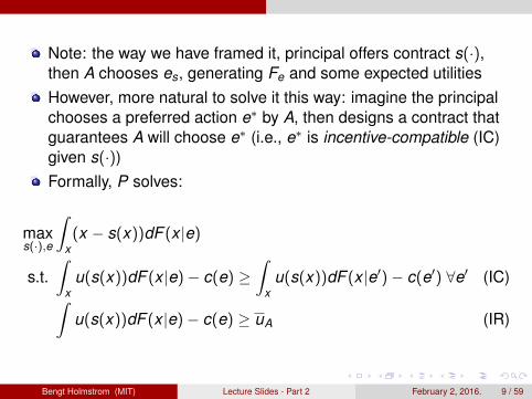
Note: the way we have framed it, principal offers contract s(·), then A chooses es, generating Fe and some expected utilities However, more natural to solve it this way: imagine the principal chooses a preferred action e ∗ by A, then designs a contract that guarantees A will choose e ∗ (i.e., e ∗ is incentive-compatible (IC) given s(·)) Formally, P solves:

max (x − s(x))dF (x |e) s(·),e x s.t. u(s(x))dF (x |e) − c(e) ≥ u(s(x))dF (x |e') − c(e') ∀e' (IC) x x

u(s(x))dF (x |e) − c(e) ≥ uA (IR)

Bengt Holmstrom (MIT) Lecture Slides - Part 2 February 2, 2016. 9 / 59

The second constraint (individual rationality, IR) assumes A has some outside option paying uA, so P ’s contract must pay at least that much We can solve this with a two-step approach:

First, for a given e, what s(x) is optimal to implement it? Let B(e) be P ’s utility under the best possible contract that implements e (Note: an optimal contract never has randomized s because P is risk-neutral and A is risk-averse) Second: what e is optimal? Find maxe B(e).

Bengt Holmstrom (MIT) Lecture Slides - Part 2 February 2, 2016. 10 / 59

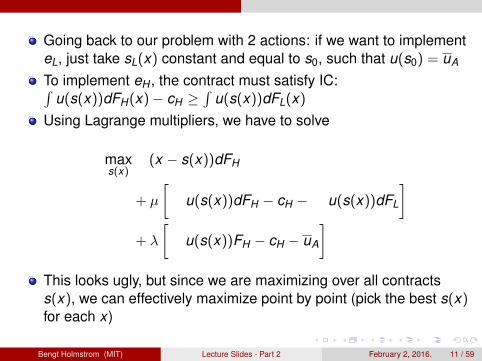
Going back to our problem with 2 actions: if we want to implement eL, just take sL(x) constant and equal to s0, such that u(s0) = uA

o implement eH , the contract must satisfy IC:TT T u(s(x))dFH (x) − cH ≥ u(s(x))dFL(x)

Using Lagrange multipliers, we have to solve

max (x − s(x))dFH s(x)

+ µ u(s(x))dFH − cH − u(s(x))dFL + λ u(s(x))FH − cH − uA

This looks ugly, but since we are maximizing over all contracts s(x), we can effectively maximize point by point (pick the best s(x) for each x)

Bengt Holmstrom (MIT) Lecture Slides - Part 2 February 2, 2016. 11 / 59

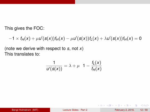
This gives the FOC:

−1 × fH (x) + µu ' (s(x))fH (x) − µu ' (s(x))fL(x) + λu ' (s(x))fH (x) = 0

(note we derive with respect to s, not x) This translates to:

1 fL(x) = λ + µ 1 − u ' (s(x)) fH (x)

Bengt Holmstrom (MIT) Lecture Slides - Part 2 February 2, 2016. 12 / 59

Lecture 4

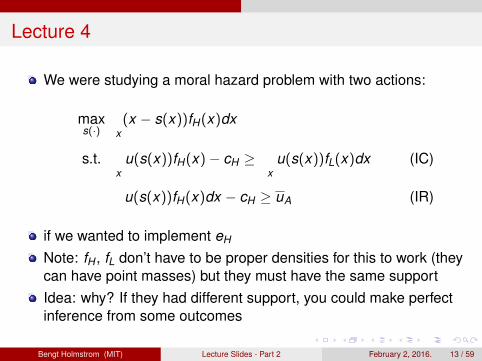
We were studying a moral hazard problem with two actions:

max s(·)

(x − s(x))fH (x)dx x

s.t. x

u(s(x))fH (x) − cH ≥ x

u(s(x))fL(x)dx (IC)

u(s(x))fH (x)dx − cH ≥ uA (IR)

if we wanted to implement eH

Note: fH , fL don’t have to be proper densities for this to work (they can have point masses) but they must have the same support Idea: why? If they had different support, you could make perfect inference from some outcomes

Bengt Holmstrom (MIT) Lecture Slides - Part 2 February 2, 2016. 13 / 59

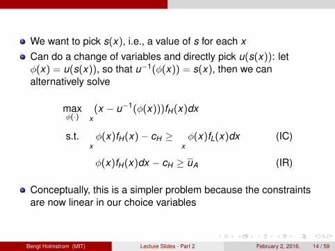
We want to pick s(x), i.e., a value of s for each x

Can do a change of variables and directly pick u(s(x)): let φ(x) = u(s(x)), so that u−1(φ(x)) = s(x), then we can alternatively solve

max φ(·)

(x − u−1(φ(x)))fH (x)dx x

s.t. x φ(x)fH (x) − cH ≥

x φ(x)fL(x)dx (IC)

φ(x)fH (x)dx − cH ≥ uA (IR)

Conceptually, this is a simpler problem because the constraints are now linear in our choice variables

Bengt Holmstrom (MIT) Lecture Slides - Part 2 February 2, 2016. 14 / 59

We obtain a Langrangian with multipliers µ for the IC constraint and λ for the IR constraint Note: if IR is not binding, P can always do better by reducing φ(x) uniformly for all x (does not affect IR), hence IR is always binding and λ > 0 Note: built into our statement that P maximizes his utility subject to IC and IR, is the assumption that if the optimal e is implemented with a program that leaves A indifferent with another action e ', he will pick whichever one is better for P

But we could frame it the other way, and maximize A’s utility subject to P ’s outside option or a market condition, and we would get the same set of results. Both programs return points on the possibility frontier of (EuA, EuP )

Bengt Holmstrom (MIT) Lecture Slides - Part 2 February 2, 2016. 15 / 59

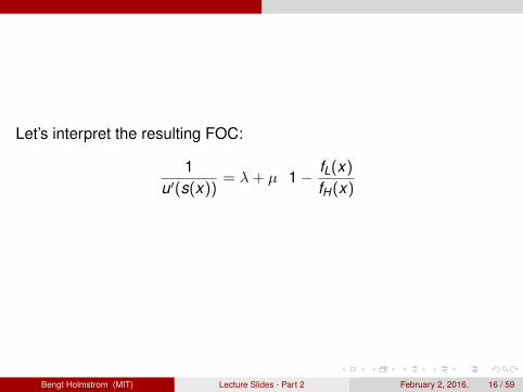
Let’s interpret the resulting FOC:

1 fL(x) = λ + µ 1 − u ' (s(x)) fH (x)

Bengt Holmstrom (MIT) Lecture Slides - Part 2 February 2, 2016. 16 / 59

Some observations: fL(x)sH (x) is decreasing in l(x) = (likelihood ratio) fH (x)

sH (x) is increasing in x iff MLRP: if x is higher, 1 − l(x) is higher by MLRP, so u ' (s(x)) is lower, so s(x) is higher by concavity of U

Note: solution is as if P is making inferences about A’s choice (pay more for signals that are more likely under high effort). But paradoxically, in equilibrium, there is actually no inference because A’s action is chosen with certainty, so P knows it If P is risk neutral, then the solution is the same if P ’s payoff is some π(x) − s(x) instead of x − s(x). It just matters that x is a signal of effort, not that it is P ’s profits.

Bengt Holmstrom (MIT) Lecture Slides - Part 2 February 2, 2016. 17 / 59

Note: if there was no incentive problem, the optimal solution would just involve 1 = λ, as in a risk sharing problem (since P is u'(s(x)) risk-neutral) This formula tells us to what extent the risk-sharing incentive is distorted by the need to incentivize A

Moral: tension in this model is between incentives and mitigating the cost of A’s risk aversion

Bengt Holmstrom (MIT) Lecture Slides - Part 2 February 2, 2016. 18 / 59

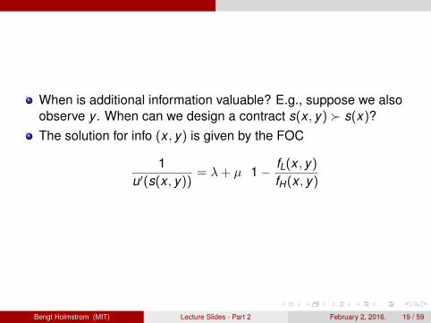
When is additional information valuable? E.g., suppose we also observe y . When can we design a contract s(x , y) > s(x)? The solution for info (x , y) is given by the FOC

1 fL(x , y) = λ + µ 1 − u ' (s(x , y)) fH (x , y)

Bengt Holmstrom (MIT) Lecture Slides - Part 2 February 2, 2016. 19 / 59

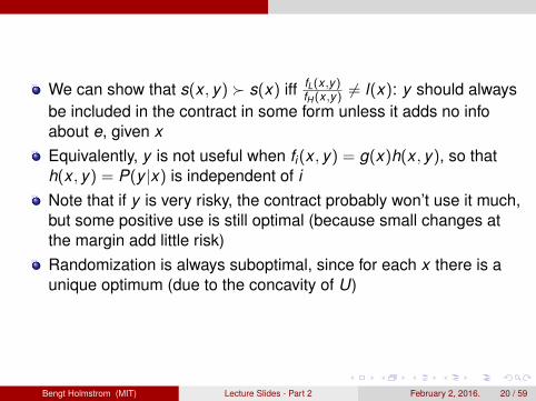
We can show that s(x , y) > s(x) iff fL(x ,y) = l(x): y should always fH (x ,y)be included in the contract in some form unless it adds no info about e, given x

Equivalently, y is not useful when fi (x , y) = g(x)h(x , y), so that h(x , y) = P(y |x) is independent of i Note that if y is very risky, the contract probably won’t use it much, but some positive use is still optimal (because small changes at the margin add little risk) Randomization is always suboptimal, since for each x there is a unique optimum (due to the concavity of U)

Bengt Holmstrom (MIT) Lecture Slides - Part 2 February 2, 2016. 20 / 59

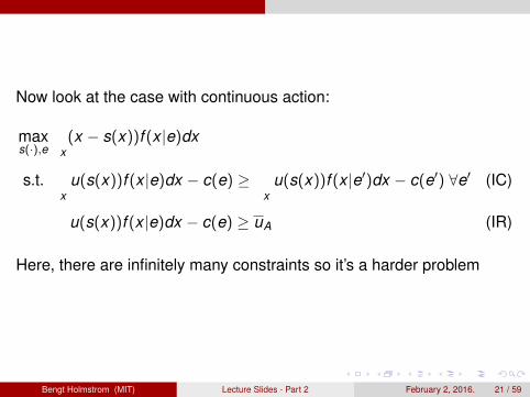
Now look at the case with continuous action:

max (x − s(x))f (x |e)dx s(·),e x

' s.t. u(s(x))f (x |e)dx − c(e) ≥ u(s(x))f (x |e ' )dx − c(e ' ) ∀e (IC) x x

u(s(x))f (x |e)dx − c(e) ≥ uA (IR)

Here, there are infinitely many constraints so it’s a harder problem

Bengt Holmstrom (MIT) Lecture Slides - Part 2 February 2, 2016. 21 / 59

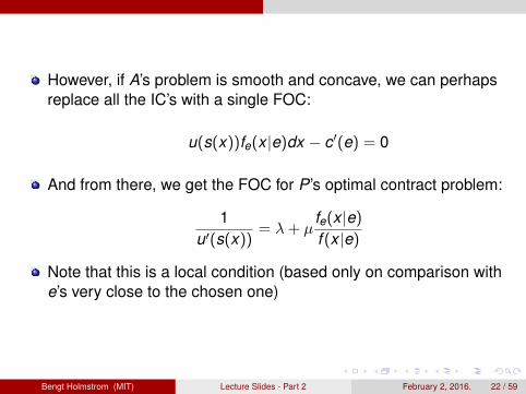
However, if A’s problem is smooth and concave, we can perhaps replace all the IC’s with a single FOC:

u(s(x))fe(x |e)dx − c ' (e) = 0

And from there, we get the FOC for P ’s optimal contract problem:

1 fe(x |e) = λ + µ

u ' (s(x)) f (x |e)

Note that this is a local condition (based only on comparison with e’s very close to the chosen one)

Bengt Holmstrom (MIT) Lecture Slides - Part 2 February 2, 2016. 22 / 59

This is the right solution if the local approach is valid But what if it’s not? Suppose that f (x |e) = N(e, σ2)

Then fe (x |e) ∝ x−e f (x |e) σ2

Plugging that into our FOC, we get a contradiction: low enough x ’s would get negative marginal utility What’s going on? There is no solution satisfying the FOC!

Bengt Holmstrom (MIT) Lecture Slides - Part 2 February 2, 2016. 23 / 59

What’s the true solution? Since the normal distribution offers potentially so much info (there are x ’s with very extreme likelihood ratios), P can incentivize A by simply punishing very hard for very bad (but unlikely) outcomes This can be done at vanishingly low cost, so we can approach the first best, but not reach it

Bengt Holmstrom (MIT) Lecture Slides - Part 2 February 2, 2016. 24 / 59

Lecture 5

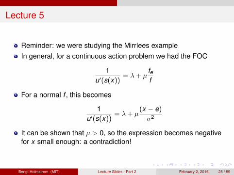
Reminder: we were studying the Mirrlees example In general, for a continuous action problem we had the FOC

1 fe = λ + µ

u ' (s(x)) f

For a normal f , this becomes

1 (x − e) = λ + µ

u ' (s(x)) σ2

It can be shown that µ > 0, so the expression becomes negative for x small enough: a contradiction!

Bengt Holmstrom (MIT) Lecture Slides - Part 2 February 2, 2016. 25 / 59

This implies there is no proper solution (any solution must satisfy the FOC) Why? The informativeness of normal signals allows us to get arbitrarily close to costless punishments (but not reach it)

Bengt Holmstrom (MIT) Lecture Slides - Part 2 February 2, 2016. 26 / 59

For comparison: compare a case where x = e + E, e = eL or eH , and E U[0, 1] Here we can implement the first best at no cost: if x ∈ [eL, eH ), then agent definitely chose eL

So we can design a contract where x ∈ [eL, eH ) is punished very hard, otherwise agent gets constant income On the equilibrium path, perfect insurance (because the agent can avoid the bad outcome with prob. 1) The key to this example: moving support allows infinitely informative signals (infinite likelihood ratio)

Bengt Holmstrom (MIT) Lecture Slides - Part 2 February 2, 2016. 27 / 59

In the normal case, by punishing only very low x ’s very hard, we get a similar result The likelihood ratio for very low x ’s becomes so extreme that it’s almost like the case with moving support But can’t fully reach first best (the limit of these contracts approaching the first best is degenerate, and has no punishment)

Bengt Holmstrom (MIT) Lecture Slides - Part 2 February 2, 2016. 28 / 59

First-best cases

When can we implement the efficient e without suffering any cost due to A’s risk aversion?

If A is risk neutral (then we can just choose s(x) = x − β to implement the optimum) If e is verifiable (then we can choose s = c0 low unless e = e ∗) If x(θ, e) and θ is verifiable (then we can back out e and we are back in the previous case) With moving support

Bengt Holmstrom (MIT) Lecture Slides - Part 2 February 2, 2016. 29 / 59

What’s wrong?

Should we be happy with this model? Agent has a fairly simple, restricted choice: just choose one-dimensional level of effort If effort is made over many days, A just chooses the mean P has infinite-dimensional control

Bengt Holmstrom (MIT) Lecture Slides - Part 2 February 2, 2016. 30 / 59

We might think that giving A a small choice space simplifies the problem, but that may not be true Giving A more options can force P to design a contract that is less manipulable, and hence simpler (For an extreme example of that, see Carroll (2015) ) E.g.: maximizing a smooth function over an interval is easier than over a large finite set Maximizing a function over a plane is often easier than over some curve embedded in the plane One-dimensional choice for A constrains him to a small family of distributions (e.g. can’t take a convex combination of available distributions)

Bengt Holmstrom (MIT) Lecture Slides - Part 2 February 2, 2016. 31 / 59

Imagine that x = e + θ where θ = E + γ

A chooses e, then observes E before choosing γ at some cost (last-minute gaming of the outcome) Even if cost of γ is high, so A constrained to very small manipulation, this breaks contracts with discontinuities (agent will game near the discontinuities)

Bengt Holmstrom (MIT) Lecture Slides - Part 2 February 2, 2016. 32 / 59

This happens in real life with target-based bonuses: If A just chooses one e, a contract that pays out iff x ≥ x ∗ (you get a bonus if you meet the quota) may be optimal, for the right distribution f But if A is making sales every day over a month, he will want to work hard as the end of the month approaches if he is close to the target, but shirk once he reaches it (or give up if too far) Clearly suboptimal now, and the culprit is A’s richer choice set Intuitively, we expect linear contracts to avoid this problem

Bengt Holmstrom (MIT) Lecture Slides - Part 2 February 2, 2016. 33 / 59

Holmstrom and Milgrom (1987) formalizes this idea for CARA utility: u(m) = −e−r(m−c(e)), and normal noise With this utility, there is no income effect (agent’s marginal incentive to work does not depend on accumulated wealth) Then, in a problem where agent chooses effort N times and sees previous outcomes before next choice, linear contract gives the right incentives Can also do in continuous time (accumulated product is Brownian motion, A chooses drift at every t)

Bengt Holmstrom (MIT) Lecture Slides - Part 2 February 2, 2016. 34 / 59

LEN Model

Let’s study the Linear Exponential Normal model (Holmstrom and Milgrom (1987) show that linear contracts are optimal in this case; this is hard, but finding the best linear contract is easy) x = e + E, E ∼ N(0, σ2) so x ∼ N(e, σ2)

u(s(x) − c(e)) = −e−r(s(x)−c(e))

s(x) = αx + β

Can consider a single outcome (given linear contract, the model is effectively separable across outcomes)

Bengt Holmstrom (MIT) Lecture Slides - Part 2 February 2, 2016. 35 / 59

Certainty Equivalent

Given a random variable X (e.g. the money payout of a lottery), the certainty equivalent CE(X ) is a certain payoff that would leave the agent indifferent compared to getting X

Formally, CE(X ) is such that u(CE(X )) = E(u(X ))

This depends on A’s attitude towards risk (more risk averse means lower CE for same lottery) For a normal distribution and CARA utility, get mean-variance decomposition: CEA(s) = E(s(x)) − 1 rVar(s(x)) − c(e)2

Bengt Holmstrom (MIT) Lecture Slides - Part 2 February 2, 2016. 36 / 59

Meanwhile CEP (s) = E(x − s(x)) = (1 − α)e − β

CEA = αe + β − 12 rα

2σ2 − c(e)

Hence total surplus is TS = e − 12 rα

2σ2 − c(e) First best effort maximizes TS, satisfies 1 = c ' (e)

Bengt Holmstrom (MIT) Lecture Slides - Part 2 February 2, 2016. 37 / 59

In practice, for a given α, A maximizes CEA and chooses e such that c ' (e) = α

If c is convex, this gives eα < eFB

Then we can choose α to maximize TS given eα, i.e., TS(α) = eα − c(eα) − 1

2 rα2σ2

1Find solution: α∗ = 1+rσ2c ''

Bengt Holmstrom (MIT) Lecture Slides - Part 2 February 2, 2016. 38 / 59

Corollary: α∗ < 1, decreasing in r (risk aversion) and σ2 (noise of signal) This model offers much more natural predictions; we would trust it more to answer new questions But note we can only do this because we have a proof that, under some conditions (richer A choices), Mirrlees-style contracts are bad and linear contracts are optimal, and we understand the difference between the settings Just saying “I don’t like the optimal solution to my original problem, so let’s just assume linear contracts” would not be kosher

Bengt Holmstrom (MIT) Lecture Slides - Part 2 February 2, 2016. 39 / 59

Aside remark: these models assume increasing cost of effort for simplicity But we can obtain the same results in models where cost of effort is U-shaped (agents intrinsically want to work up to some point): if we need them to work more than that, at the margin it is the same problem Too many papers claiming these models are irrelevant because they assume agents don’t like working

Bengt Holmstrom (MIT) Lecture Slides - Part 2 February 2, 2016. 40 / 59

Lecture 6

Reminder: we provided a justification for looking at linear contracts (Holmstrom and Milgrom 1987) We then found the optimal linear contract, characterized by

1α = c ' (e(α)) and α = 1+r σ2c ''

Bengt Holmstrom (MIT) Lecture Slides - Part 2 February 2, 2016. 41 / 59

Where does this come from? α = c ' (e(α)) just comes from A’s IC condition Then, deriving with respect to α, 1 = c '' (e(α))e ' (α) de 1 = c '' is how much more A works if I increase the commission a da little Substituting these into the derivative of TS, we find α∗

Bengt Holmstrom (MIT) Lecture Slides - Part 2 February 2, 2016. 42 / 59

Multi-tasking

So far we studied a one-activity model where the cost of providing A with incentives is burdening A with risk In multi-tasking models, A has several activities P may want to give more incentives for activities that he can monitor well (less noise means A suffers less from risk) Incentives, even for perfectly monitored activities, may be distorted if cost function is not separable Idea: if I can monitor job 1 well and 2 badly, I want to give more incentives for 1 But not to the efficient level: else 1 will crowd out too much 2

Bengt Holmstrom (MIT) Lecture Slides - Part 2 February 2, 2016. 43 / 59

Suppose A can invest effort into increasing quality and quantity x1 = e1 + E1 is quality, x2 = e2 is quantity B(e1, e2) = p1e1 + p1e2 is P ’s payoff from (e1, e2)

C(e1, e2) is A’s cost of (e1, e2)

(e1, e2 may interact in the cost function, e.g., if it is C(e1 + e2) with C convex, doing more e1 increases the marginal cost of e2 and vice versa)

Bengt Holmstrom (MIT) Lecture Slides - Part 2 February 2, 2016. 44 / 59

P designs a contract s(x1, x2) = αx1 + αx2 + β

(Again, if we assume exponential utility, ..., then linear contracts are optimal) So P solves:

max B(e1, e2) − C(e1, e2) − α1,α2,β

1 rα2

1σ2 12

s.t. α1 = ∂c ∂e1

(IC1)

α2 = ∂c ∂e2

(IC2)

Bengt Holmstrom (MIT) Lecture Slides - Part 2 February 2, 2016. 45 / 59

Note: we are not exactly solving P ’s problem, but instead maximizing total surplus This is OK because the two problems are equivalent We can also drop the IR condition because optimal α’s are independent of the preferred pie distribution, and adjusting β is how we divide the pie (thanks to exponential utility)

Bengt Holmstrom (MIT) Lecture Slides - Part 2 February 2, 2016. 46 / 59

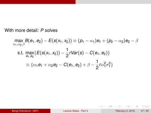
With more detail: P solves

max B(e1, e2) − E(s(x1, x2)) ≡ (p1 − α1)e1 + (p2 − α2)e2 − β α1,α2,β

1 s.t. max{E(s(x1, x2)) − rVar(s) − C(e1, e2)}e1,e2 2

1 ≡ {α1e1 + α2e2 − C(e1, e2) + β − rα12σ1

2}2

Bengt Holmstrom (MIT) Lecture Slides - Part 2 February 2, 2016. 47 / 59

To solve, go back to the total surplus problem and derive with respect to α1 and α2, getting FOCs:

∂TS ∂e1 ∂e2= (p1 − C1) + (p2 − C2) − rα1σ2 = 01α1 α1 α1

∂TS ∂e1 ∂e2= (p1 − C1) + (p2 − C2) = 0 α2 α2 α2

Then plug in the IC conditions and their versions derived with respect to αi

Bengt Holmstrom (MIT) Lecture Slides - Part 2 February 2, 2016. 48 / 59

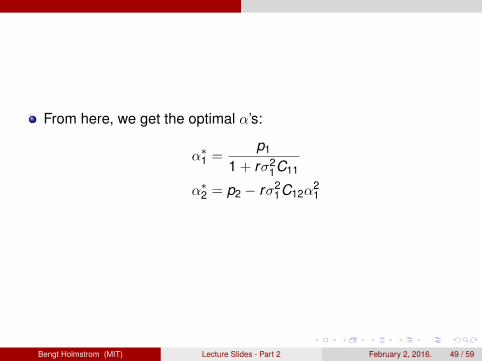
From here, we get the optimal α’s:

p1α ∗ = 1 1 + r σ1

2C11

α ∗ 2 = p2 − rσ1

2C12α12

Bengt Holmstrom (MIT) Lecture Slides - Part 2 February 2, 2016. 49 / 59

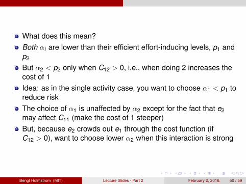
What does this mean? Both αi are lower than their efficient effort-inducing levels, p1 and p2

But α2 < p2 only when C12 > 0, i.e., when doing 2 increases the cost of 1 Idea: as in the single activity case, you want to choose α1 < p1 to reduce risk The choice of α1 is unaffected by α2 except for the fact that e2 may affect C11 (make the cost of 1 steeper) But, because e2 crowds out e1 through the cost function (if C12 > 0), want to choose lower α2 when this interaction is strong

Bengt Holmstrom (MIT) Lecture Slides - Part 2 February 2, 2016. 50 / 59

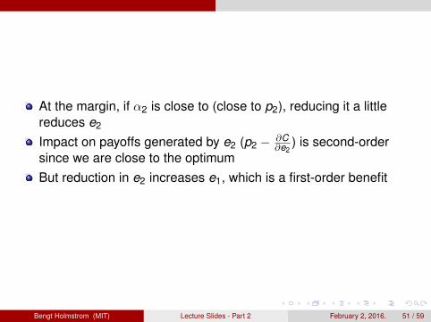
At the margin, if α2 is close to (close to p2), reducing it a little reduces e2

Impact on payoffs generated by e2 (p2 − ∂C ) is second-order ∂e2 since we are close to the optimum But reduction in e2 increases e1, which is a first-order benefit

Bengt Holmstrom (MIT) Lecture Slides - Part 2 February 2, 2016. 51 / 59

Moral of the story: low-powered incentives are good when activities are badly monitored When A has multiple activites that vary in the quality of monitoring, P should make incentives weakest for the poorly monitored activities, but also make all incentives low so poorly monitored jobs don’t get crowded out by the well monitored In some examples, could even want no incentives (fixed wage) This idea has big real-world implications

Bengt Holmstrom (MIT) Lecture Slides - Part 2 February 2, 2016. 52 / 59

Multi-task Lab

Up to now, we were in a model where P has as many levers in the contract as A has jobs So P can choose how to incentivize each activity (choose both α1 and α2), and the tension is between incentives and insurance against risk But in many real-life jobs, A has a lot of activities: vector (e1, . . . , en)

And P only has access to a few performance measures So A always has opportunities to game the measures using certain ei ’s that are well-rewarded

Bengt Holmstrom (MIT) Lecture Slides - Part 2 February 2, 2016. 53 / 59

E.g.: A is a teacher, can teach 100 different topics P has two measures: class grades and standardized exam The moral will be: in this world, we want low-powered incentives even if A is risk-neutral Beyond some point, increasing incentives will just lead to A doing too much of tasks undesired by P

E.g. “teaching to the test”

Bengt Holmstrom (MIT) Lecture Slides - Part 2 February 2, 2016. 54 / 59

E.g.: imagine that B(e) = e is P ’s activity (e.g. coding) (ek )k=1,...,K are private activities (e.g. using the computer to chat, watch videos) A’s cost is C(e + k ek ) − k vk (ek ) (A enjoys private activities, but they may increase the cost of coding by distracting A) P observes x = e + E and pays s(x) = αx + β

Suppose also that P can exclude some tasks (e.g. block Youtube on the company network) How to design the optimal contract (α, β, exclusions)?

Bengt Holmstrom (MIT) Lecture Slides - Part 2 February 2, 2016. 55 / 59

� FOCs:

α = C' (e + ek ) k

' k (ek ) = C' v = α

Note: this means that, given α, total effort e + k ek is constant! Exclusions simply transfer effort from an excluded task ek to e

Bengt Holmstrom (MIT) Lecture Slides - Part 2 February 2, 2016. 56 / 59

So should P just exclude all private activities? No Exclude ek iff it generates less total surplus than transferring to the job Exclude k iff vk (ek ) < ek

(Remember P can always adjust pie through β, so efficient to make A happy if at low cost: pay you less and let you use Youtube) Then we still have to choose the optimal α, but note that choice of what tasks to exclude is conditional on α

v(ek )If the vk are concave, then ek will be declining in α, so ek increasing in α, so task exclusions will decrease in α

(If incentives are strong, A will mostly ignore Youtube because reward for work is high; if they are weak, A will shirk a lot unless Youtube is blocked)

Bengt Holmstrom (MIT) Lecture Slides - Part 2 February 2, 2016. 57 / 59

Before moving on to the next topic: a reminder of why we can study moral hazard problems as problems of maximizing total surplus P is solving: max EUP subject to (IC) and EUA ≥ uA (IR) or equivalently CEA ≥ u−1(uA)

Under exponential utility, if a point (CEP , CEA) is achievable, then (CEP + β, CEA − β) is achievable too: just transfer β no matter what the state, or in other words make a new contract s2(x) = s(x) − β for all x

Hence, if there is a contract maximizing CEP + CEA, then it is optimal to implement essentially that contract no matter the desired distribution of the pie, and then just change the β to achieve different distributions

Bengt Holmstrom (MIT) Lecture Slides - Part 2 February 2, 2016. 58 / 59

Without exponential utility, the idea is less clear because certainty equivalents are not as handy, and the optimal contract changes depending on desired distribution due to income effects But it is still true that we can essentially solve by maximizing TS subject to IC and IR

Bengt Holmstrom (MIT) Lecture Slides - Part 2 February 2, 2016. 59 / 59

MIT OpenCourseWare https://ocw.mit.edu

14.124 Microeconomic Theory IV Spring 2017

For information about citing these materials or our Terms of Use, visit: https://ocw.mit.edu/terms.