Zed3DA compact reference for 3d computer

graphics programming

by Sébastien Loisel 1994, 1995, 1996

2

Zed3D - A compact reference for 3dcomputer graphics programming

Copyright 1994, 1995, 1996 by Sébastien Loisel All RightsReserved, version 0.95β

Zed3D is a document about computer graphics, more particularly real-time 3dgraphics. This document should be viewed as a practical reference for a first andperhaps second course in computer graphics.

The original Zed3D document grew out of my work notes. As a matter of fact, theoriginal Zed3D, up to version 0.61beta, was my work notes. As such, it wasmessy, incomplete and often incorrect. I have attempted to correct this a bit now. Istill consider these my work notes, but I have added more formal introductorymaterial which was not in the original document.

In this document, I will attempt to describe various aspects of computer graphicsin a clear, useful and complete fashion. You will find quite a bit of the theoreticalaspects, copies of the calculations and proofs I made and so forth.

3

However, there is the painful fact that I am merely a student, trying to mark myterritory in the university work, and since this work does not serve that purposevery well, Zed3D will oftentimes be lacking in areas that I wish I had more time todocument. Also, I will attempt to distribute another nice portable graphics enginein the future, but that's only if I can find the time to make it.

Also, please note that this document and any accompanyingdocumentation/software for which I am the author should not be considered publicdomain. You can redistribute this whole thing, unmodified, if no fee is charged forit, otherwise you need the author's written permission. Also I am not responsiblefor anything that might happen anywhere even if it's related directly or indirectly tothis package. If you wish to encourage my effort, feel free to send me a 10$ check,which will be considered to be your official registration. If you're really on abudget, I would appreciate at least a postcard. At any rate, please read theregistration paragraph below. There have been rumours about a 0.70 version ofZed3D about. This would be a fake, versions between 0.63 and 0.79 do not exist,and have never existed.

Contact information

If you wish to contact me for any reason, you should be using the following snail-mail address or my e-mail address. Given that snail-mail addresses tend to be morestable over time, you might try it if I don't answer to your electronic messages.

E-Mail Address: zed@cs.mcgill.ca

Snail Mail Address:For the 1995-1996 school year, I will reside at:

Sébastien Loisel3436 Aylmer Street, apartment 2Montréal, Québec, CanadaPostal Code: H2X 2B6

Otherwise, it is possible to reach me at:

Sébastien Loisel1 J.K. LaflammeLévis, Québec, CanadaPostal Code: G6V 3R1

Registration

4

If you want to register your copy of Zed3D for life, and be able to use the sourcein any way you want, even commercial (though commercial utilization of thedocumentation [this file] still requires the written permission of the author), youcan send me a cheque of US$10.00. For more information, please consult the fileregister.frm, which should have come with this document. If you are experiencingdifficulties with registration or if the file register.frm is missing, please mail me andwe will work something out.

Overview

I am trying to put a bit more structure into this document. As such, this is how it ismeant to be structured at this moment.

The first section is heavily mathematical. It deals with transformations by and atlarge. First are discussed linear and affine transformations, which are used to spinand move stuff in space in a useful fashion, then is discussed and justified theperspective transforms. These two sections are very theoretical, but are requiredfor proper understanding of the later sections.

Then there will follow a section dealing specifically with applications of thepreceding theory. Namely, rotation matrices and their inverse and object hierarchy.

The third "section" concerns itself mainly with rendering techniques. These arebecoming less and less important for several reasons. The complexity of theproblem is of course not in the rendering section of the pipeline. Second, the recenttrend has pushed the rendering part of the pipeline into cheap video hardwarewhich can do the job fast and effectively while the CPU is off to some other, moreimportant task. Eventually, we can hope that transforming objects will also bemade a part of popular low-cost hardware, but that remains to be seen. As it isnow, this is often the job of either the CPU, or sometimes we might wish to givethis job to a better co-processor (for example, a programmable DSP).

Fourthly, an attempt will be made to describe a few shading models and visiblesurface determination techniques. Shading models are but loosely related to theway the polygons are drawn. Visible surface determination depends somewhatmore on the way polygons are drawn, and is often implemented in hardware.

The following section deals with a few of the computer graphics related problemsthat are often encountered, such as error tolerant normal computation, the problemof finding a correctly oriented normal, polygon triangulation and quaternions torepresent orientations, which are especially useful in keyframe animations.

5

There is also a short glossary and even shorter bibliography. [1] is a highlyrecommended reading to anyone intending to do serious computer graphics. Thereis a lot of overlap between Zed3D and [1], though [1] doubtlessly contains a greatdeal more information than this text. However, Zed3D does cover a rare fewtopics which are more or less well covered in [1] (example: quaternions).

Of course, a lot of topics remain to be covered, such as real-time collisiondetection, octrees and other data structures. However, I unfortunately do not havethe time to write all of that down for the general public.

6

Table of Contents

Zed3D - A compact reference for 3d computer graphicsprogramming...............................................................................2

Contact information..............................................................................3Registration..........................................................................................3

Overview.........................................................................................................4

Table of Contents.........................................................................6

Vector mathematics.....................................................................10Introduction.....................................................................................................10

On notation..........................................................................................10Vector operations............................................................................................11

Exercises..............................................................................................12Answers...............................................................................................13

Alcoholism and dependance.............................................................................13Exercises..............................................................................................14Answers...............................................................................................15

On a plane (and of motion sickness)................................................................. 15Exercises..............................................................................................16Answers...............................................................................................17

Orthonormalizing a basis..................................................................................17

Matrix mathematics.....................................................................19Introduction.....................................................................................................19Matrix operations.............................................................................................19

Exercise...............................................................................................21Answer................................................................................................. 22

Matrix representation & linear transformations.................................................22

Affine transforms.........................................................................25

7

Introduction.....................................................................................................25Affine transformations......................................................................................25

Exercise...............................................................................................26Affine transform combination and inversion......................................................27

Exercise...............................................................................................27Answer................................................................................................. 28

Applications of linear transformations.........................................30Introduction.....................................................................................................30World space, eye space, object space, outer space............................................30Transformations in the hierarchy (or the French revolution)..............................31Some pathological matrices..............................................................................31

Perspective...................................................................................34Introduction.....................................................................................................34A simple perspectively incorrect projection......................................................35The perspective transformation........................................................................35Theorems.........................................................................................................38Other applications............................................................................................39

Constant Z...........................................................................................41Texture mapping equations revisited.....................................................41Bla bla.................................................................................................. 43

Reality strikes.................................................................................................. 44

Interpolations and approximations...............................................46Introduction.....................................................................................................46Forward differencing........................................................................................46Approximation function...................................................................................48

Polynomial Splines......................................................................51Introduction.....................................................................................................51Basic splines....................................................................................................51Parametrized splines.........................................................................................54Uniform splines................................................................................................54Examples.........................................................................................................57Frequently used uniform cubic splines..............................................................60

Hermite splines.....................................................................................60Bézier splines.......................................................................................61Convex hull..........................................................................................62

8

Bernstein polynomials...........................................................................63Uniform nonrational B-spline................................................................64

Catmull-Rom splines: a non-uniform type of spline...........................................65

Rendering....................................................................................66Introduction.....................................................................................................66The point.........................................................................................................66Lines................................................................................................................69Polygon drawing..............................................................................................70

Visible surface determination......................................................73Introduction.....................................................................................................73Back-face culling.............................................................................................74Sorting.............................................................................................................75Painter's algorithm and depth sorting................................................................77Z-Buffering......................................................................................................79Binary Space Partitioning.................................................................................80

Lighting models...........................................................................84Introduction.....................................................................................................84Lighting models...............................................................................................84Smooth shading...............................................................................................86Texture mapping & variants on the same theme................................................89

Computer graphics related problems...........................................91Introduction.....................................................................................................91Generating edge normals..................................................................................91Triangulating a polygon...................................................................................92Computing a plane normal from vertices..........................................................93Generating correctly oriented normals for polyhedra........................................94Polygon clipping against a line or plane............................................................95

Quaternions..................................................................................97Introduction.....................................................................................................97Preliminaries....................................................................................................98Conversion between quaternions and matrices..................................................99Orientation interpolation..................................................................................99

9

Antialiasing..................................................................................101Introduction.....................................................................................................101Filtering...........................................................................................................101Pixel accuracy.................................................................................................. 102Sub-pixel accuracy...........................................................................................104Time antialiasing, a.k.a. motion blur................................................................. 105Mipmapping.....................................................................................................106

Uniform Mipmapping...........................................................................107Nonuniform Mipmapping.....................................................................108Summed area tables..............................................................................109

Bi-linear interpolation......................................................................................110Tri-linear interpolation.....................................................................................111

Glossary.......................................................................................112

Bibliography................................................................................115

10

Vector mathematics

Introduction

Linear algebra is a rather broad yet basic field of college level mathematics. It isbeing taught (or should be at any rate) early on to students in mathematics andengineering. However simple it is, it's a lengthy topic to discuss. And since thisdocument is not meant as a mathematics textbook, I will only give here the gist ofthe thing.

If you need further information on the topic, browse your local library for linearalgebra books and somesuch, or go ask a professor. As of now, I'm not makingany bibliography for this, but if and when I do, I'll try to give a few decentreferences.

The purpose of linear algebra in 3d graphics is to implement all the rotation,skewing, translation, changes in coordinates, and otherwise affine transformationsto 3d object. The applications range from merely rotating an object about its ownsystem of axis to object hierarchy, moving cameras and can be extended throughquaternions for rotation interpolation and such.

As such, linear algebra is something that is essential for any 3d graphics engine tobe useful.

Since my prime concern is 3d graphics, I will give only whatever theory isabsolutely necessary for that topic. What's below extends in a vary natural way ton dimensions, n>3, except for cross product, which is a bit awkward.

On notation

I will frequently use the sigma symbol for sums, for example, something like this:

∑0≤i≤nai

which stands for

a0+a1+a2+a3+...+an.

11

More generally, the notation

∑i∈ Iai

stands for “sum of all ai for all i in I”. This notation will not be used frequently inthis work. Notation from more advanced math might be used especially in proofs.

Vector operations

A vector in 3d is noted (a,b,c) where a, b and c are real numbers. Similarly, avector in 2d is noted (a,b) for a, b real numbers. The vector for which allcomponents are null deserves a special mention, it is usually noted 0, with theproper number of components implied in the notation but not explicitly given.

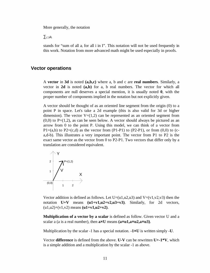
A vector should be thought of as an oriented line segment from the origin (0) to apoint P in space. Let's take a 2d example (this is also valid for 3d or higherdimension). The vector V=(1,2) can be represented as an oriented segment from(0,0) to P=(1,2), as can be seen below. A vector should always be pictured as anarrow from 0 to the point P. Using this model, we can think of a vector fromP1=(a,b) to P2=(c,d) as the vector from (P1-P1) to (P2-P1), or from (0,0) to (c-a,d-b). This illustrates a very important point. The vector from P1 to P2 is theexact same vector as the vector from 0 to P2-P1. Two vectors that differ only by atranslation are considered equivalent.

1

2

Y

X

1 2

P=(1,2)

(0,0)

V

Vector addition is defined as follows. Let U=(u1,u2,u3) and V=(v1,v2,v3) then thenotation U+V means (u1+v1,u2+v2,u3+v3). Similarly, for 2d vectors,(u1,u2)+(v1,v2) means (u1+v1,u2+v2).

Multiplication of a vector by a scalar is defined as follow. Given vector U and ascalar a (a is a real number), then a××U means (a××u1,a××u2,a××u3).

Multiplication by the scalar -1 has a special notation. -1××U is written simply -U.

Vector difference is defined from the above. U-V can be rewritten U+-1*V , whichis a simple addition and a multiplication by the scalar -1 as above.

12

Multiplication of two vectors has no intuitive meaning. However, two types of"multiplications" of vectors are usually defined, which have little relation to theusual real number multiplication.

The first is dot product. U dot V (usually noted U•• V) yields a real number (not avector). (u1,u2,u3)• (v1,v2,v3) means u1××v1+u2××v2+u3××v3. Similarly for 2dvectors, (u1,u2)• (v1,v2)≡u1×v1+u2×v2. Note that the 1d case corresponds tonormal multiplication of real numbers in a certain way.

Vectors have a length, defined as follow. The length (or module, or norm) ofvector U is written |U| and has the value of (U•• U)1/2. If the length of a vector isone, the vector is said to be of unit length, or a unit or normal vector.Multiplying a vector V by the scalar 1/|V| is called normalizing a vector, becauseit has the effect of making V a unit vector. In the 1d case, length simplifies toabsolute value, thus the notation |U|.

Dot product is also used to define angle. U•• V=|U|××|V|××Cosθθ, where θ is the anglebetween U and V. Incidentally, if |U|=1 then this simplifies to |V|×Cosθ, which isthe length of the projection of V onto U. It is of note that U•V is 0 if and only ifeither θ is π/2+2kπ or |U|=0 or |V|=0. Assuming |U| and |V| are not 0, this meansthat if U•V is 0, then U and V are perpendicular, or orthogonal.

The second product usually defined on vectors is the cross product. U cross V(usually noted U××V) is defined using matrix determinant and somesuch. Basically,(u1,u2,u3)×(v1,v2,v3) is (u2v3-u3v2, u3v1-u1v3, u1v2-u2v1).

It is demonstrable that the cross product of two vectors is perpendicular to the twovectors and has a length of |U||V|Sinθθ. The fact that it is perpendicular hasapplications which we will see later.

Exercises

Q1 - Do the following vector operations:

a) (1,3,2)+(3,5,6)

b) 1.5×(3,4,2)

c) (-1,3,0)• (2,5,2)

d) |(3,4,20/3)|

e) U•V where |U|=2, |V|=3 and the angle between U and V is 60 degrees

f) (1,2,3)×(4,5,6)

13

Q2 - Which vectors satisfy the equation U• (1,1,1)=0?

Answers

A1 - a) (4,8,8)

b) (4.5,6,3)

c) 13

d) 25/3

e) 3

f) (-3,6,-3)

A2 - All vectors that satisfy u1+u2+u3=0. Since the dot product is 0, this meansall vectors that are perpendicular to U. Incidentally, these vectors cover the wholeplane and nothing but the plane for which the normal is (1,1,1). All the vectors ofthe said plane can be expressed as p(1,-1,0)+r(0,-1,1) [for example] for some realnumbers p and r. This last notation is also known as a local coordinates system forthe u1+u2+u3=0 plane.

Alcoholism and dependance

Given a set of vector U0, U1, U2, ... , Un, these vectors are said to be linearlyindependent if and only if the following is true:

a0××U0+a1××U1+...+an××Un=0 implies that (a0,a1,a2, ... , an)=0.

If there exists at least one solution for which (a0, a1, a2, ...,an) is not zero, thenthere exists an infinity of them, and the vector are said to be linearly dependant.

The geometric interpretation of that is as follows. In 3d, three vectors are linearlyindependent if none of them are colinear and all three of them are not coplanar.(Colinear means on the same line, coplanar means on the same plane). Any morethan 3 vectors in 3d and they are certain to be linearly dependant.

For two vectors, in 2d or 3d, they are said to be linearly independent if they are notcolinear. 3 or more vectors in 2d are always linearly dependant.

If a set of vectors are linearly independent, they are said to form a basis. 2 linearlyindependent vectors form the basis for a plane, and 3 linearly independent vectorsform the basis for a 3d space.

14

The term orthogonal is very frequently used to describe perpendicular vectors. Ifa basis is made of orthogonal unit vectors (unit vectors are vectors of norm 1), thebase is said to be orthonormal . Orthonormal basis are the most useful kind intypical 3d graphics. If a basis is not orthonormal, it "skews" the space, where if thevectors are not unit, it "stretches" and/or "compresses" the space.

Each space has a so-called canonical basis, the basis we intuitively find simplest.For 3d space, that basis is made of the vectors (1,0,0), (0,1,0) and (0,0,1).Similarly, the canonical basis for 2d space is (1,0) and (0,1). Note that since a basisis a set of vectors, it would be more formal to enclose the list of vectors in curlybraces, for example, {(2,3) , (-1,0)}.

The vectors of the canonical basis are traditionally noted i, j and k for 3d space ori and j for 2d space. This leads us to introduce another notation.

If vector (a,b,c) is said to be expressed in basis pqr , then it means that the vectoris a×p+b×q+c×r. Note that a, b and c are scalars and p, q and r are vectors, thusthis combination (formally referred to as linear combination) is defined asdiscussed earlier. If pqr are ijk, this translates to a×i+b×j+c×k or(a,0,0)+(0,b,0)+(0,0,c) or (a,b,c).

However, if pqr is not ijk, the matter is different. For example (assuming pqr isexpressed in ijk space), if p=(1,1,0), q=(0,1,1) and r=(1,0,1), then the vector(a,b,c) in pqr space means (a,a,0)+(0,b,b)+(c,0,c)=(a+c,a+b,b+c) in ijk space.What we just did is called a change of basis. We took a vector that was expressedin pqr space and expressed it in ijk space.

Note: normally, to specify which space a vector is expressed in, we should writethe space in subscript. Example: as in the preceding paragraph, (a,b,c) is writteneither (a,b,c)pqr or (a+c,a+b,b+c)ijk depending on whether we want it in pqr or ijkspace. This notation will help avoid many mistakes.

It would be possible for pqr to be expressed in some other base than the canonicalbase. If that were the case, and if the objective would be to express vector (a,b,c)in ijk space, then it might require several transformations to get there.

For simplicity's sake in the further parts of this document, we will extend ourdefinition of vectors to allow for not only real number components, but also vectorcomponents. This means that (a,b,c)pqr expressed in pqr space (a×p+b×q+c×r) canbe written as (a,b,c)pqr•• (p,q,r) ijk .

Exercises

Q1 - Are the vectors (1,2,0), (4,2,4) and (-7,-4,-8) linearly independent?

15

Q2 - Say vector U=(1,3,2)pqr is expressed in pqr space, where pqr expressed in ijkspace is (1,2,0)ijk, (2,0,2)ijk, (0,-1,-1)ijk. Express U in ijk space.

Q3 - Using Question 2's values for p, q and r, and the vector V expressed in ijkspace as (1,1,1), can you express V in pqr space?

Answers

A1 - No

A2 - (7,0,4)ijk

A3 - (1/3, 1/3, -1/3) - this exercise is in fact called an inverse transform, which willbe described later.

On a plane (and of motion sickness)

There are several ways to define a plane in 3d. The first one I will present is usefulbecause it can be used to represent a plane in n dimensional space, even for n>3.

First you need two linearly independent vectors to form a basis. Call them U andV. Then, if you take a×U+b×V for all possible values of a and b (them being realnumbers of course), you generate a whole plane that goes through the origin ofspace. If you want to displace that plane in space by vector W (e.g. you want thepoint pointed to by W to be part of the plane), then a××U+b××V+W will generatethe desired plane. (Proof, for a=b=0, it simplifies to W, thus the point at W is partof the plane).

Note that the above equation can be written (a,b)•• (U,V)+W. As such it can beviewed as a change of basis, from the canonical basis of 2d space to whateverspace U and V's basis is.

Another way for defining a plane that only works in 3d is as follows. (Note, in ndimensional space, this will define a n-1 dimensional object). As was seen earlier, ifA•X=0, then A and X are perpendicular (A and X are vectors). Furthermore, for agiven A, if you take all X's that satisfy the equation, you get all points in a certainplane. A is generally called normal to the plane, although the literature frequentlyassumes that the normal is also of unit length, which is not necessary (though Amust not be the null vector). The values of X that satisfy the plane equation giveninclude X=0, since A•0=0 for any value of A. Thus, that plane passes through theorigin.

16

If one wants a plane that does not pass through the origin, one should proceed asfollows. (This uses an intuitive form of affine transformations, described in depthlater). First, find out the displacement vector K that describes the position of theplane in relation to the origin. Thus, if you subtract K from all the points in theplane, the plane ends up at the origin, and we can use the definition above. Thus,the new definition of the plane is A• (X-K)=0.

To make this a bit more explicit, let A=(A,B,C) and X=(x,y,z) and K=(k1,k2,k3).Then the plane equation can be rewritten as: A×(x-k1)+B×(y-k2)+C×(z-k3)=0. Alittle algebra allows us to rewrite it as A×x+B×y+C×z=-A×k1-B×k2-C×k3. Bysetting D=-A×k1-B×k2-C×k3, we can make one more rewrite, which is the finalform: A××x+B××y+C××z=D.

It is important to remember that multiplying both side of the equation by aconstant does not change the plane. Thus, plane x+y+z=1 is the same as plane2x+2y+2z=2.

Note that in this last representation, (A,B,C) is the normal vector to the plane.The last equation can also be re-written A•• X=D. It would also be easy todemonstrate the following, but I will not do it. For any point P, (A•• P-D)/|A| is thesigned distance to the plane A•X=D. The sign can help you determine on whatside of the plane that the point P lies on. If it is 0, P is on the plane. If it is positive,P is in the direction that the normal points to. If it is negative, P is on the sideopposite of the normal. This has application in visible surface determination(namely, back face culling).

Also note that if |A|=1, then the signed distance equation simplifies to A•P-D.

It is easy to demonstrate that the equation for a line in n-space, for any integervalue of n>0, is t××U+W, where U is a vector parallel to the line and W is a pointon the line. As t takes all real values, we generate a line.

Exercises

Q1 - Given the basis U=(1,3,2) and V=(2,2,2), and the position vector W=(1,1,0),find the position in 3d space of the point (3,2) in UV space.

Q2 - Express the plane described in Q1 in the form Ax+By+Cz=D

Q3 - Find the signed distance of point (4,2,4) to the plane using the answer forquestion 2.

Q4 - Given two basis vectors for a plane, P and Q, in 3d space, and a positionvector for the plane, R, plus the direction vector of a line, M, that passes throughorigin, find the pq space point of intersection between the line and the plane.

17

Answers

A1 - (8,14,10)

A2 - x+y-2z=2 (hint : remember that the cross product of U and V is perpendicularto both U and V).

A3 - -4/(61/2)≅ -1.633 - this means that the point (4,2,4) is in the directionopposite of (1,1,-2) from the plane x+2-2z=2.

A4 - See the perspective chapter on texture mapping.

Orthonormalizing a basis

Sometimes we might have a basis B which is meant to be orthonormal, but due toaccumulation in roundoff error in the computer, the vectors are slightly off the unitlength and not quite perpendicular. Then it is useful to have a way of finding anorthonormal basis O from our basis B while making sure that O and B are "verysimilar" in a certain sense.

The meaning of "very similar" can be made explicit easily. Let B be the basis (b1,b2, ..., bn) for a n-dimensional space (bi's are vectors). Let O be the basis (o1, o2,..., on). Then, we measure the "similitude" of O and B by taking Max(|oi-bi|), thatis, the greatest difference between the same vector in O and B. The closer thisnumber is to 0, the more similar O and B are. The method given below willgenerate O from B such that the similitude is small enough (note that it will notnecessarily be the smallest possible, it will simply be small enough).

The process in n-dimensional space is as follows. Let

v1=b1

vn=bn-∑1≤i<n(bn•oi)oi

on=vn/|vn|

Then, the basis O is orthonormal and has good similitude with the basis B. (Proofis left as an exercise. Hint: find an upper bound on the similitude as a function ofthe maximum of the dot product between two vectors of the basis B and as afunction of the length of the vectors in the basis B. Proof of orthogonality comesfrom examining vn closely. Unit norm of the vectors of the basis is obvious.)

Explicitly for the 3d case, this simplifies to:

o1=b1/|b1|

18

v2=b2-(b2•o1)o1

o2=v2/|v2|

v3=b3-(b3•o1)o1-(b3•o2)o2

o3=v3/|v3|

19

Matrix mathematics

Introduction

Matrices are a tool used to handle a great deal of linear combinations in ahomogeneous way. The operations on matrices are so defined as to ease whatevertask you want to do with them. Be it expressing a system of equations, or makinga change of basis, to some peculiar uses in calculus.

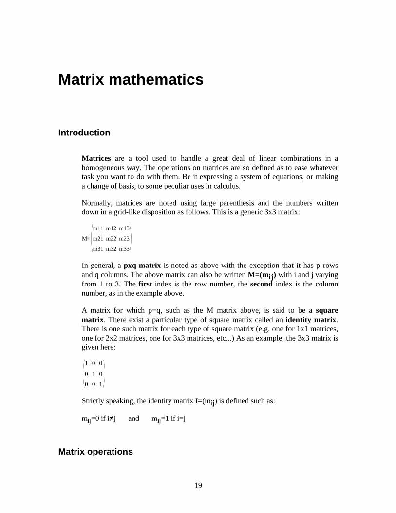
Normally, matrices are noted using large parenthesis and the numbers writtendown in a grid-like disposition as follows. This is a generic 3x3 matrix:

M

m11

m21

m31

m12

m22

m32

m13

m23

m33

In general, a pxq matrix is noted as above with the exception that it has p rowsand q columns. The above matrix can also be written M=(mij ) with i and j varyingfrom 1 to 3. The first index is the row number, the second index is the columnnumber, as in the example above.

A matrix for which p=q, such as the M matrix above, is said to be a squarematrix . There exist a particular type of square matrix called an identity matrix .There is one such matrix for each type of square matrix (e.g. one for 1x1 matrices,one for 2x2 matrices, one for 3x3 matrices, etc...) As an example, the 3x3 matrix isgiven here:

1

0

0

0

1

0

0

0

1

Strictly speaking, the identity matrix I=(mij ) is defined such as:

mij=0 if i≠j and mij=1 if i=j

Matrix operations

20

Matrix addition is defined as follows. Given 2 matrices A=(aij ) and B=(bij ) ofsame dimension pxq, then U=(uij )=A+B is defined as being (uij )=(aij +bij ).

Matrix multiplication by a scalar is defined also as follows. Given the matrix Mand a scalar k, then the operation U=(uij )=k×M is defined as uij=k×mij .

Matrix multiplication is a bit more involved. It is defined using sums, as follows.Given matrix A of dimension pxq, and matrix B of dimension qxr, the productC=AxB is given by:

cij=∑1≤k≤q(aik×bkj)

More explicitly, for example, we have, for A and B 2x2 matrices:

c11=a11×b11+a12×b21

c12=a11×b12+a12×b22

c21=a21×b11+a22×b21

c22=a21×b12+a22×b22

(Note: ∑1≤k≤q(aik×bkj) means "sum of (aik×bkj) for k varying from 1 to q.")

It is important to notice that matrix multiplication is not commutative in thegeneral case. For example, it is not true that A×B=B×A with A and B matrices inthe general case, even if A and B are square matrices. Matrix multiplication is,however, associative (ie, A×(B×C)=(A×B)×C) and distributive (ie,A(B+C)=AB+AC).

The identity matrix has the property that, for any matrix A, A×I=I×A=A (I is theneutral element of matrix multiplication).

Matrix transposition of matrix A, noted AT, reflects the A matrix along the greatdiagonal. That is, say A=(aij ) and AT=(bij ), then we have bij=aji .

There are also other interesting operations you can do on a matrix, however theyare much, much more involved. As of now, I am not willing to get too deeply intothis. The topics of interest are matrix determinant (which has a recursivedefinition) and matrix inversion. I will content myself by giving one definition ofmatrix determinant and one way of finding matrix inverse. Note that there are atleast a couple of different definitions for determinant, though they usually boildown to the same thing. Also, there are many ways of finding the inverse of amatrix, I will contend myself with presenting only one method. Strict definitionswill be given, for more extensive coverage, consult a linear algebra book.

21

Given a matrix M=(mij ), of size 1x1, the determinant (sometimes written detM)is defined as D=m11. For matrices of size nxn with n>1, the definition is recursive.First, pick an integer j such that 1≤j≤n. For example, you could pick j=1.

D=mj1×Cj1+mj2×Cj2+...+mjn×Cjn

The Cij are the cofactors of M - they require a bit more explaining, which follows.

First let us define the minor matrix Mij of matrix M. If M is a nxn matrix, then theMij matrix is a (n-1)x(n-1) matrix. To generate the Mij matrix, remove the ith lineand jth column from the M matrix.

Second what interests us is the cofactor Cij , which is defined to be:

Cij=(-1)i+j×detMij

As an example, the determinant of the 2x2 matrix M is m11×m22-m12×m21, andthe determinant of a 3x3 matrix M is

D3x3= m11×(m22×m33-m23×m32)

- m12×(m21×m33-m23×m31)

+ m13×(m21×m32-m22×m31)

Given a matrix A, the inverse of the matrix, noted A-1 (if it exists), is such that A×A-1=A-1×A=I. It is possible that a matrix has no inverse.

To inverse the matrix, we will first define the adjacent matrix of A, which we willcall B=(bij ). Let Cij denote the i,j cofactor of A. Then, we have:

bij=Cij

Which completely defines the cofactor matrix B. The inverse of A is then:

A-1=(1/detA)×BT

Another method of inverting matrices, which might be preferable for numericalstability reasons but will not be discussed here, is the Gauss-Jordan method.

Exercise

Q1 - Compute the product of these two matrices:

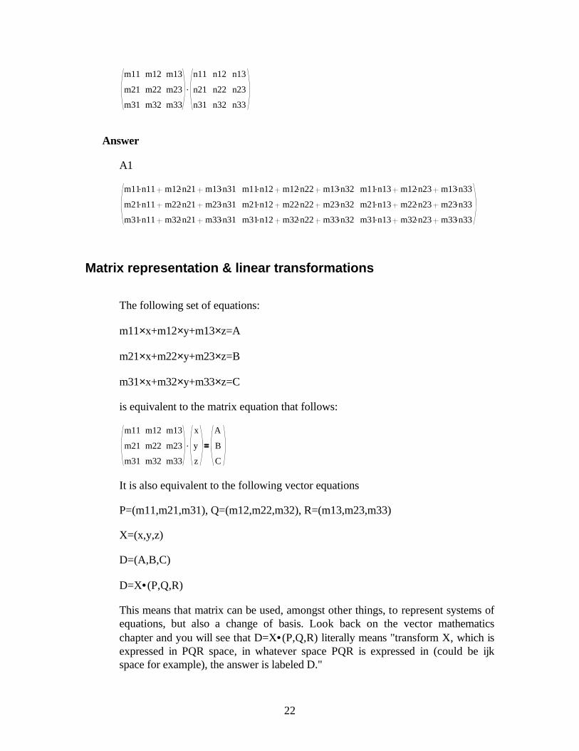
22

.

m11

m21

m31

m12

m22

m32

m13

m23

m33

n11

n21

n31

n12

n22

n32

n13

n23

n33

Answer

A1

.m11n11 .m12n21 .m13n31

.m21n11 .m22n21 .m23n31

.m31n11 .m32n21 .m33n31

.m11n12 .m12n22 .m13n32

.m21n12 .m22n22 .m23n32

.m31n12 .m32n22 .m33n32

.m11n13 .m12n23 .m13n33

.m21n13 .m22n23 .m23n33

.m31n13 .m32n23 .m33n33

Matrix representation & linear transformations

The following set of equations:

m11×x+m12×y+m13×z=A

m21×x+m22×y+m23×z=B

m31×x+m32×y+m33×z=C

is equivalent to the matrix equation that follows:

.

m11

m21

m31

m12

m22

m32

m13

m23

m33

x

y

z

A

B

C

It is also equivalent to the following vector equations

P=(m11,m21,m31), Q=(m12,m22,m32), R=(m13,m23,m33)

X=(x,y,z)

D=(A,B,C)

D=X• (P,Q,R)

This means that matrix can be used, amongst other things, to represent systems ofequations, but also a change of basis. Look back on the vector mathematicschapter and you will see that D=X• (P,Q,R) literally means "transform X, which isexpressed in PQR space, in whatever space PQR is expressed in (could be ijkspace for example), the answer is labeled D."

23

The matrix form can also be written as follows:

M×X=D

This is also called the linear transformation of X by M. In this case, if the matrixM is invertible, then we can premultiply both sides of the equality by M-1, asfollows:

M-1×M×X=M-1×D

And, knowing that M-1×M=I (and that matrix multiplication is associative as wesaw before), we substitute into the above:

I×X=M-1×D

And knowing that I×X=X, we finally get:

X=M-1×D

That is a very elegant, efficient and powerful way of solving systems of equations.The difficulty is of course finding M-1. For example, if we know M, D but not X,we can use the above to find X. This is what should be used to solve question 3 inchapter "Alcoholism and dependance". For 3d graphics people, this is the singlemost useful application of matrix inversion: sometimes you have a point in ijkspace, and you want to express them in pqr space. However, you don't originallyhave ijk expressed in pqr space, but you have pqr expressed in ijk space. You willthen write the transformation of a point from pqr space to ijk space, then find theinverse transformation as just described and then inverse transform the point tofind it's position in pqr space.

Another very interesting aspect is as follows. If we have a point P to betransformed by matrix M, and then by matrix N. What we have is:

P'=M×P

P''=N×P'

By combining these two equations, we get

P''=N×(M×P)

However, by associativity of matrix multiplication, we have:

P''=(N×M)×P

24

If for instance, we plan to process a great many points through these twotransformations in that particular order, it is a great time saver to be able to firstcalculate A=N××M , and then simply evaluate P''=A ××P for all P's, instead of firstcalculating P' then P''. In linear transformations terminology, A is said to be thelinear combination of M and N.

25

Affine transforms

Introduction

As of now, we have seen linear transformations. Linear transformations can beused to represent changes of basis. However, they fail to take into account possibletranslation, which is of top priority to 3d graphics. An affine transform is, roughly,a linear transform followed by a translation (or preceded, though it is more usefulfor 3d graphics to picture them as being followed by the translation instead).

Affine transformations

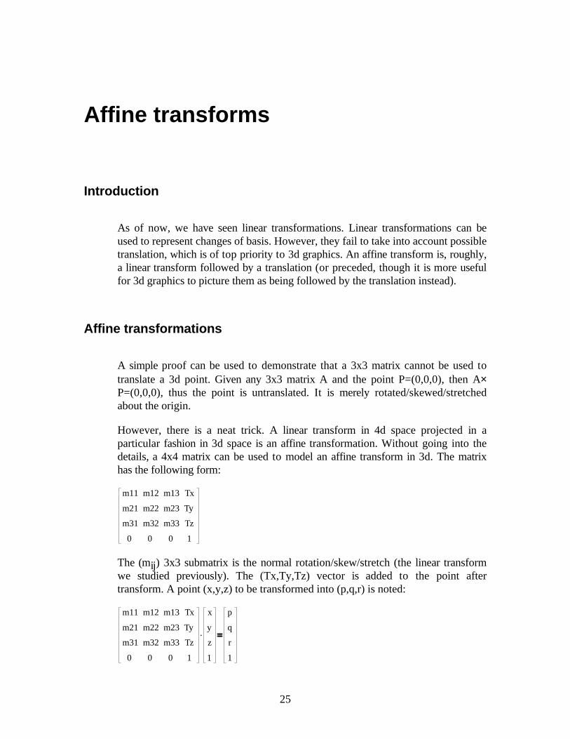
A simple proof can be used to demonstrate that a 3x3 matrix cannot be used totranslate a 3d point. Given any 3x3 matrix A and the point P=(0,0,0), then A×P=(0,0,0), thus the point is untranslated. It is merely rotated/skewed/stretchedabout the origin.

However, there is a neat trick. A linear transform in 4d space projected in aparticular fashion in 3d space is an affine transformation. Without going into thedetails, a 4x4 matrix can be used to model an affine transform in 3d. The matrixhas the following form:

m11

m21

m31

0

m12

m22

m32

0

m13

m23

m33

0

Tx

Ty

Tz

1

The (mij ) 3x3 submatrix is the normal rotation/skew/stretch (the linear transformwe studied previously). The (Tx,Ty,Tz) vector is added to the point aftertransform. A point (x,y,z) to be transformed into (p,q,r) is noted:

.

m11

m21

m31

0

m12

m22

m32

0

m13

m23

m33

0

Tx

Ty

Tz

1

x

y

z

1

p

q

r

1

26

Another way of modelling affine transform is to use the conventional 3x3 matrixwe were using previously, and to add a translation vector after each lineartransform. The advantage of this is that we do not do unnecessary multiplicationsfor translation and also the bottom row of the 4x4 matrix which is (0,0,0,1) thatcan be optimized out. However, the advantage of using the 4x4 matrix on theconceptual level (not on the implementation level) is that you can then computeaffine transformation combinations and inversions, the exact same way that wewere doing in the previous section.

A very special note. Sometimes it becomes useful to distinguish vectors frompoints in space. A vector is not affected by a translation, while a point is. Toillustrate our example, think of a plane and a plane's normal. Let's say we takethree points in the plane, rotate them and translate them, we get a new plane.These points are affected by the translation and the rotation. However, the planenormal is only affected by the rotation.

When using affine transforms with the 4x4 matrix above, a vector (x,y,z) isrepresented by (x,y,z,0) and a point is represented by (x,y,z,1). This way, whenyou multiply a vector by a 4x4 matrix, the translation does not affect it (try it andyou will see), while a point is affected by it.

This very important aspect gives meaning to the various operations on points andvectors. Sums and differences of vectors are still vectors. (E.g.(a,b,c,0)+(d,e,f,0)=(a+d,b+e,c+f,0), which is still a vector). Difference of twopoints is a vector. This is very important:

(a,b,c,1)-(d,e,f,1)=(a-d,b-e,c-f,0) (a vector since the last component is 0)

Sum of two points has no meaning. (It can be given one, but for us it has nomeaning). This is illustrated this way: (a,b,c,1)+(d,e,f,1)=(a+d,b+e,c+f,2). The lastcomponent is no 0, so it's not a vector, and it's not 1 so it's not a point. (We coulduse homogeneous coordinates and give it a meaning, but this is totallyunimportant.)

Sum of a vector and a point is a point. Subtracting a vector from a point yields apoint, also.

Exercise

Prove that the sum of a vector and a point is a point and not a vector or undefined,and prove that the difference of a point and a vector is a point as opposed to avector or undefined. What is the meaning if any of multiplying a point by a scalar?a vector by a scalar?

27

Affine transform combination and inversion

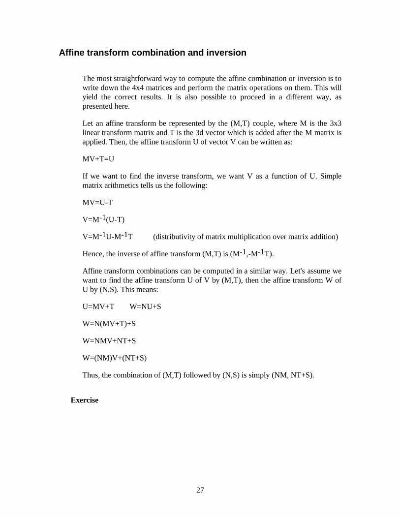
The most straightforward way to compute the affine combination or inversion is towrite down the 4x4 matrices and perform the matrix operations on them. This willyield the correct results. It is also possible to proceed in a different way, aspresented here.

Let an affine transform be represented by the (M,T) couple, where M is the 3x3linear transform matrix and T is the 3d vector which is added after the M matrix isapplied. Then, the affine transform U of vector V can be written as:

MV+T=U

If we want to find the inverse transform, we want V as a function of U. Simplematrix arithmetics tells us the following:

MV=U-T

V=M-1(U-T)

V=M-1U-M-1T (distributivity of matrix multiplication over matrix addition)

Hence, the inverse of affine transform (M,T) is (M-1,-M-1T).

Affine transform combinations can be computed in a similar way. Let's assume wewant to find the affine transform U of V by (M,T), then the affine transform W ofU by (N,S). This means:

U=MV+T W=NU+S

W=N(MV+T)+S

W=NMV+NT+S

W=(NM)V+(NT+S)

Thus, the combination of (M,T) followed by (N,S) is simply (NM, NT+S).

Exercise

28

Q1- Assume we have three points P={P1, P2, P3} in 3d and the three pointsQ={Q1, Q2, Q3} also in 3d. These points are read from a special device and theirreal location in 3d space is known with very good precision (note: this means thereis no perspective distortion in our data). We know that the points P and Q are thevery same points, except that they're viewed from a different location. This meansthat the points in Q are the points in P transformed by some affine transform A.However, we do not know which points in Q correspond to which points in P. (ie,Q1 is not necessarily the affine transform of P1, it might be the affine transform ofP2 or P3). You can assume that the points P1, P2 and P3 form a nondegeneratetriangle whose sides all measure a different length.

Q2- We have roughly the same problem as in Q1, except now we have n>3 pointsP=(P1, P2, P3, ..., Pn) and the corresponding Q=(Q1, Q2, Q3, ..., Qn). Can youfind a way to compute the affine transform while minimizing error? (Warning - thisis difficult.)

Answer

A- First step is to determine which point in Q correspond to which point in P.Since they're the same points viewed from different angles, we can assume thelinear transform part of the affine transform is orthogonal, therefore it preserveslengths and angles. We can use that to find which points should be associated. Tothis purpose, let u=P2-P1, v=P3-P1. Then, find the i,j, k such that |u|=|Qj-Qi|,|v|=|Qk-Qi|. Since we assumed the sides of the triangle have all different lengths,there is only one i,j,k which will work. We can simply try all 6 combinations untilone works. Then, we know that P1 corresponds to Qi, P2 corresponds to Qj, P3corresponds to Qj.

Now, let R1, R2, R3 be Qi, Qj, Qk respectively (this is to simplify notation a bit).We need a third vector, which we generate as follows. Let w=u×v. Note that, asseen in the last section, u, v and w are vectors and therefore are not affected bytranslations. Let the affine transform A be represented by (M,T) a 3x3 matrix and a3d vector. Let p=R2-R1, q-R3-R1 and r=p×q.

Then, we have that p=Mu, q=Mv, r=Mw (prove it, especially the last one).

This can be re-written as

M(u|v|w)=(p|q|r)

where (u|v|w) denotes the 3x3 matrix formed by taking the vectors u, v and w andputting them in as column vectors. Then, we can compute W by calculating

M=(p|q|r)(u|v|w)-1 (*)

29

Now we have computed the M matrix. We need to compute the T vector. Weknow that R1=MP1+T, hence T=R1-MP1 and we are done.

A2- The general outline is similar to A1, except that at step (*), instead of usingthe conventional matrix inversion, we need a so-called pseudoinverse matrix,denoted M+, which is

M+=(MTM)-1MT

This matrix is a generalization of the conventional matrix inverse. It minimizesmean square error in overconstrained sets of equations like we have here. See [2]for more information on this topic. Note that finding which Qi correspond towhich Pj is slightly more difficult, but a similar method can be used. Also note thatthe T vector should be computed for all points and then averaged to minimizeerror. Additionally, we were generating a w vector which was the cross product ofu and v. Now we might require something analogous to generate a linearlyindependent component else the matrix will be degenerate and inversion will behighly error prone. This especially if the points are suspected to be coplanar.

30

Applications of lineartransformations

Introduction

In this section we will discuss the applications of the linear transformation theorywe saw in the previous sections. When doing 3d graphics, the usual situationoccurs. We have a description of one or more objects. We have their locations andorientations in space, relative to some point of reference. We move them around,rotate them, usually about their own coordinate system. The camera might also bemoving, rotating and such. In that case, it is likely that we have an orientation andposition for the camera object itself. We would also like that the eye points in thedirection of (0,0,1) in camera space, and that up be (0,1,0) in camera space.

Orientation and position will be given by an affine transform matrix. The (mij )submatrix gives orientation and the 4th column has the translation vector.

World space, eye space, object space, outer space

First off we are going to require a global system of reference for all the objects.This is usually called "World space". An affine transform that describes anobject's position and orientation usually does so in relation to world space (this isgenerally not true for hierarchical structures, as we will see later). This introducesa new concept; a matrix A, representing an affine transform that takes an objectfrom space M to space N (in our example, M is object space and N is world space)is usually noted AN←←M . This has the natural tendency to make us combine theaffine transform from right to left instead of left to right, which is correct.

The most typical example is as follows. We have an object and its affine transformAWorld←Object. We also have a camera position and orientation given by CWorld←

Camera. In that case, the first thing we want to do is invert the transform CWorld←

Camera to find the CCamera←World transform. Then you will be transforming the pointsPi in the object with CCamera←World×AWorld←Object×Pi=MCamera←Object×Pi.

As a helper, notice that the little arrows make a lot of sense, as shown below:

31

Camera←World, World←Object, which concatenates intuitively to Camera←World←Object or simply Camera←Object. Thus, the above transformationtransforms from object space to camera space directly. One merely calculatesMCamera←Object=CCamera←World×AWorld←Object and multiplies all Pi's with is.

Transformations in the hierarchy (or the French revolution)

It may be useful to express an object A's position and orientation relative not to theworld, but to some other object B. This way, if B moves, A moves along with it.In plain words, if we say "The television is resting 2 centimeters above the desk onits four legs", then moving the desk does not require us to change our "2centimeters above the desk" position - it is still 2 centimeters above the desk as it ismoving along with the desk (careful not to drop it). On the other hand, if we hadsaid "The television is 1 meter above the floor" and "The desk is 95 centimetersabove the floor", and then proceed to move the desk up 1 meter, then the positionof the desk is "1m95 above the floor". Additionally, we have to edit the position ofthe television and change it to "The television is 2 meters above the floor". Noticethe difference between these two examples.

This can be implemented very easily the following way. Make an affine transformthat describes orientation and position of television in relation to the desk. This iscalled ADesk←Television. Then we have an orientation and position for the desk, givenby BWorld←Desk. Notice that this last affine transform is relative to world space. Wethen of course have the mandatory CWorld←Camera which we invert to find the CCamera

←World transform. We then proceed to transform all points in the television tocamera space, and also all points from the desk to camera space. The former isdone as follows:

CCamera←World×BWorld←Desk.×ADesk←Television×Pi.

Notice again how the arrows concatenate nicely. The points on the desk aretransformed with this:

CCamera←World×BWorld←Desk.×Qi.

Again, the arrows make all the sense in the world.

Some pathological matrices

32

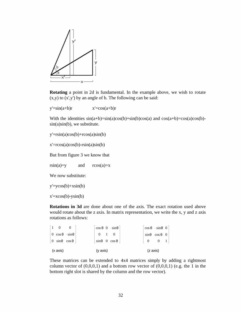
Rotating a point in 2d is fundamental. In the example above, we wish to rotate(x,y) to (x',y') by an angle of b. The following can be said:

y'=sin(a+b)r x'=cos(a+b)r

With the identities sin(a+b)=sin(a)cos(b)+sin(b)cos(a) and cos(a+b)=cos(a)cos(b)-sin(a)sin(b), we substitute.

y'=rsin(a)cos(b)+rcos(a)sin(b)

x'=rcos(a)cos(b)-rsin(a)sin(b)

But from figure 3 we know that

rsin(a)=y and rcos(a)=x

We now substitute:

y'=ycos(b)+xsin(b)

x'=xcos(b)-ysin(b)

Rotations in 3d are done about one of the axis. The exact rotation used abovewould rotate about the z axis. In matrix representation, we write the x, y and z axisrotations as follows:

1

0

0

0

cosθ

sinθ

0

sinθ

cosθ

cosθ

0

sinθ

0

1

0

sinθ

0

cosθ

cosθ

sinθ

0

sinθ

cosθ

0

0

0

1

(x axis) (y axis) (z axis)

These matrices can be extended to 4x4 matrices simply by adding a rightmostcolumn vector of (0,0,0,1) and a bottom row vector of (0,0,0,1) (e.g. the 1 in thebottom right slot is shared by the column and the row vector).

33

If you want, you can always specify the orientation of an object using three angles.These are formally referred to the Euler angles. Unfortunately, these angles arenot too useful for many reasons. If two angles change with constant speed, theobject will definitely not rotate with constant speed. Also, sometimes, a problemknown as gimbal lock occurs, where you suddenly lose one degree of freedom(this looks like the object's rotation in a direction stops, to start again in anotherstrange direction). Furthermore, the angles are not relative to object coordinatesystem nor world coordinate system.

Thus it is preferable to specify object orientation with an orientation matrix. Whenrotation about a world axis is desired, the orientation matrix is premultiplied byone of the above rotation matrices, and when a rotation about an object axis isdesired, the orientation matrix is postmultiplied by one of the above rotationmatrices. Note that it is possible to rotate about an arbitrary vector and/orinterpolate between any two given orientations when using quaternions, which iscovered in a later chapter..

34

Perspective

Introduction

Perspective was a novelty of the Renaissance. It existed a long time before but hadbeen forgotten by the western civilizations until that later time. As can be seenfrom paintings before Renaissance, artists had a very poor grasp of how thingsshould appear on a painting. The edges from tables and desks were not drawnconverging to an "escape point", but rather all parallel. This gave these paintingsthe peculiar feeling they have when compared to more modern, more perspective-correct paintings.

Perspective is the name we give to that strange distortion that happens when youtake a real-life 3d scene (your garden) and take a picture of it. The flowers in theforeground appear larger than the barn in the background. This particular effect issometimes referred to as foreshortening. Other effects come into play, such asfocus blur (very likely, you were either focussed on the flowers or the barn; onelooks clear, the other is very fuzzy), light attenuation, atmospheric attenuation,etc...

We know today that light rays probably aren't moving in a straight line at all. Evenin the vacuum, they oscillate a bit. When travelling through matter, it is deviated allthe time, split, reflected and all sorts of other nonsense. Sometimes it can be usefulto model all these nice effects, however, they are not always necessary ordesirable. One thing is for sure, a perfect or near-perfect simulation of all that weknow about light today would be tremendously CPU-intensive, and would requirean incredible amount of work on the software end of the project.

In normal, day-to-day life, when you're significantly larger than an atom butsignificantly smaller than a planet, light is usually pretty linear. It travels in straightrays, only bending at discrete points that are more or less easy to calculate,definitely more than the fuzzy way light bends in a prism.

A further simplification that we can make is that light only reflects diffusely on theobjects around you. This is usually the case, unless you come up to a highlypolished or metallic surface where you can see your reflection. But the usual desk,bed, snake and starships are pretty dull in appearance, with perhaps a diffusehighlight from where the light is coming from.

35

Another simplification we usually make comes from the fact that light bounces offeverything and eventually starts coming from about all direction with a lowintensity. This is often called the ambient light. Some further optimizations, morehacks than actual physical observations, will make you go faster and still lookgood.

A simple perspectively incorrect projection

The most simple projection is an affine transform from 3d to 2d, sometimesreferred to as parallel projection. As an example, the transform (x,y,z)→(x,y)transforms the point (x,y,z) in 3d to the point (x,y) in 2d, is such a transform.Another simple example is the (x,y,z)→(x+z,y+z) transform. The problem with thisis, no matter how far or close in z the object is, it always appears the same size onthe screen. This, or a variant of this, is true for all of the parallel projections. Theseprojections are called parallel because parallel lines in 3d remain parallel onceprojected in 2d. The image below is a parallel projected cube:

The perspective transformation

36

The perspective transformation (or perspective projection) is incredibly simpleonce you know it, but it is often good to know where it comes from. We will putto use some of the assumptions we previously stated.

The first assumption we made is that light goes in a straight line. This is greatbecause it will allow us to make maximum use of all the linear math we have learntsince high-school.

What we have to realize is, for the eye to see an object, light has to travel from theobject to the eye. Since light travels in a straight line, it has to either go straight tothe eye or bounce off a few reflective surfaces before getting there. However, sincewe are assuming there are no such reflective surfaces in the environment, the onlypossibility left is that the light comes straight from the object to the eye. This line isformally referred to as a projector.

Another way doing it is the exact inverse. Starting from the eye, shoot a ray in adirection until it hits something. That is what you are seeing in that direction.

Obviously, we are not going to shoot an infinite number of rays in all direction, wewould never even start generating an image if we did that. The usualapproximation is to shoot a finite amount of rays spread over an area in anarbitrary manner.

There is another matter that needs to be taken care of. In reality, the image will besent to screen, paper or some other media. This means that, in our model, the lightdoes not reach the eye, it stops at the screen or paper, and that is what we display,so that reality takes over for the rest of the way and carries real light rays from thescreen to the real eyes. This poses a problem of finding where the light raysintersect the screen or paper.

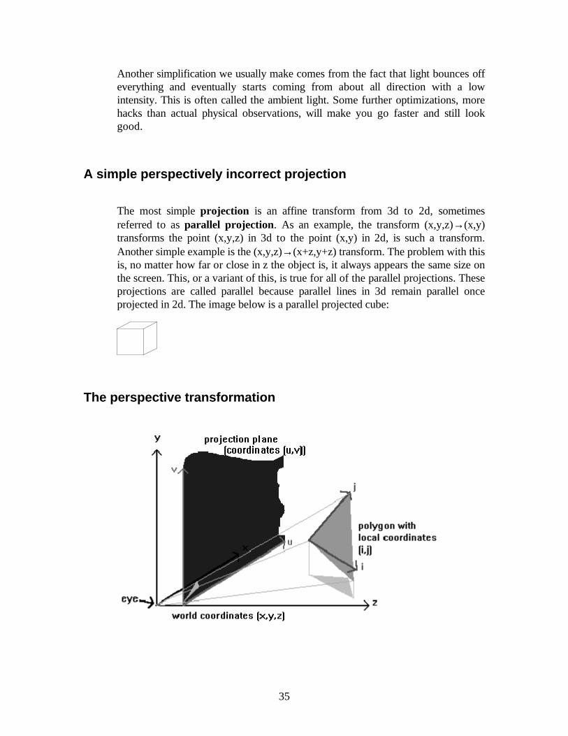
Using the material in the previous section, we are able to transform all objects tocamera space, where forward is (0,0,1) and up is (0,1,0) and the eye is at (0,0,0).We still do not know where in space the screen lies. We will have to make a fewmore assumptions, that it is in front of the eye, perpendicular to the eye directionwhich is (0,0,1), and flat. The distance at which it lies is still undecided. We willjust work with the constant k for the distance, then see what value of k interests usmost. The eye is formally referred to as center of projection, and the plane thesurface of projection.

37

Since it is flat, it lies on a plane. The plane equation in question is Ax+By+Cz=Das seen before, where (A,B,C)=(0,0,1) is the plane normal. Thus the planeequation is z=D. The distance from the eye is thus D, and we want it to be k, sowe set D=k. The plane equation is therefore z=k. We set a local basis for thatplane with vectors i=(1,0,0) and j=(0,1,0) and position W=(0,0,k). The planeequation is thus (a,b)• (i,j)+W. (a,b) are the local coordinates on the plane. Theyhappen to correspond to the (x,y) position on the plane in 3d space because (i,j)for the plane is the same as (i,j) for the world.

The question we now ask ourselves is this: given a point that is reflecting light, saypoint (x,y,z), what point on screen should be lit that crosses the light ray from(x,y,z) to the eye, which is at (0,0,0).

Here we will use the definition of the line in n space we mentioned before (namely,tV+W). Since the light ray goes from (x,y,z) to (0,0,0), it is parallel to the vector(x,y,z)-(0,0,0)=(x,y,z). Thus, we can set V=(x,y,z). (0,0,0) is a point on the line, sowe can set W=(0,0,0). The line equation is thus t(x,y,z).

We now want the intersection of the line t(x,y,z) with the plane z=k. Setting t=k/z(assuming z is nonzero), we find the following: k/z(x,y,z)=(k×x/z,k×y/z,k). Thispoint has z=k thus it is in the plane z=k, thus it is the intersection of the plane z=kand the line t(x,y,z).

Trivially from that, we find that the point (a,b) on screen are (k×x/z,k×y/z). Thus,

(x,y,z) perspective projects to (k××x/z, k××y/z).

A small note on aspect ratios. Sometimes, a screen's coordinate system is"squished" on one axis. In this case, it would be wise to "expand" one of thecoordinates to make it larger to compensate for the screen being squished. Forexample, if the screen pixels are 3/4 as wide as they are high, it would be wise tomultiply the b component of screen position by 3/4, or the a component by 4/3.This can be computed using 2 different values of k instead of the same. Forexample, use k1=k and k2=ratio*k. Then, the perspective projection equation is:

(x,y,z) perspective projects to (k1××x/z, k2××y/z).

Referring again to physics, only one point gets to be projected to a particular pointon screen. That is, closer objects obscure objects farther away. It will thus beuseful to do some form of visible surface determination eventually. Another specialcase is that anything behind the eye does not get projected at all. Thus, if beforethe projection, z≤0, do not project. The image below is a perspective projectedcube. Compare with the parallel projected cube of the preceding section.

38

Theorems

The following theorems are not always entirely obvious, but they are of great helpwhen doing 3d graphics. I will attempt to give the reader rough proofs andjustifications when possible, usually they will be geometrical proofs for they aremuch more natural in this case. These proofs are not very formal, but formalproofs are not hard to find, just much less natural.

A line in 3d perspective projects to a line in 2d. However, line segments sometimeshave erratic behavior. The proof is as follows. If the object to project is a line, thenthe set of all projectors pass through the center of projection, which is a point, andthe line. Since projector are linear, they all belong to the plane P defined by the lineand the point. Thus, the projection will lie somewhere in the intersection of theplane P and the projection plane. However, the intersection of two planes isgenerally a line. Here follows the exception.

If the planes are parallel, since the projection plane does not pass on the eye, theyare necessarily disjoint. The projection in this case is nothing.

A line segment generally projects to a line segment. First, the only portion of theline segment that needs to be projected is the portion for which z>0, as seenpreviously. If the segment crosses z=0, it should be cut at z=0, and only the z>0section kept. Second, the projectors for a line segment all lie in a scaled up trianglewhich intersects the projection plane in a particular way, and the intersection of atriangle and a plane is always a line segment.

Next proof is the proof that a n-gon (a n-sided polygon, example, triangles are 3-gons, squares are 4-gons, etc...) projects to a n-gon. It can be demonstrated thatany polygon can be triangulated in a finite set of triangles, so the proof is kept totriangles only. Also, if the n-gon crosses z=0, it should be cut at z=0, and only thez>0 section kept.

A triangle projects to a triangle. The projectors of a triangle all lie in an infinitelyhigh tetrahedron, and the intersection of an infinitely high tetrahedron and theprojection plane, in the non-infinite direction is always a triangle.

39

In a similar line of thought, the set of all projectors of a sphere form a cone. Theintersection of the cone with the projection plane can form any conic. Namely, ahyperbola, an ellipse or a circle. If the sphere contains the origin, the projectionfills the whole projection plane.

Other applications

By not losing sight of the idea behind the projection, one can accomplish muchmore than what has been just described. One example is texture mapping. Often, apolygon will be drawn on screen, but some properties of the polygon (say color forexample) changes across the polygon in 3d space. When this happens, we want toknow what point from the polygon we are currently drawing. An application ofthis is texture mapping.

Texture mapping involves taking the point on screen, finding the projector thatgoes through it and finding the intersection of that projector with the polygon. Wethen have a point in 3d space. However, it is usually much more useful to make alocal 2d coordinate system for the plane containing the polygon and make theproperty a function of the location in that 2d coordinate system. This is what I didbelow in the snapshot of the screen from my math software.

40

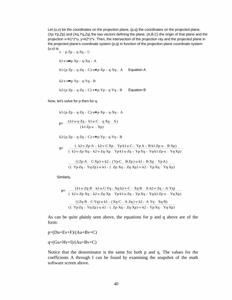
Let (u,v) be the coordinates on the projection plane, (p,q) the coordinates on the projected plane, (Xp,Yp,Zp) and (Xq,Yq,Zq) the two vectors defining the plane, (A,B,C) the origin of that plane and the projection x=k1*z*u, y=k2*z*v. Then, the intersection of the projection ray and the projected plane in the projected plane's coordinate system (p,q) in function of the projection plane coordinate system (u,v) is:

z .p Zp .q Zq C

..k1 z u .p Xp .q Xq A

..k1 ( ).p Zp .q Zq C u .p Xp .q Xq A Equation A

..k2 z v .p Yp .q Yq B

..k2 ( ).p Zp .q Zq C v .p Yp .q Yq B Equation B

Now, let's solve for p then for q.

..k1 ( ).p Zp .q Zq C u .p Xp .q Xq A

p=( )...k1 u q Zq ..k1 u C .q Xq A

( )..k1 Zp u Xp

..k2 ( ).p Zp .q Zq C v .p Yp .q Yq B

q=( )...k2 v Zp A ...k2 v C Xp ...Yp k1 u C .Yp A ...B k1 Zp u .B Xp

( )...k2 v Zp Xq ...k2 v Zq Xp ...Yp k1 u Zq .Yp Xq ...Yq k1 Zp u .Yq Xp

( )..( ).Zp A .C Xp v k2 ..( ).Yp C .B Zp u k1 .B Xp .Yp A

( )..( ).Yp Zq .Yq Zp u k1 ..( ).Zp Xq .Zq Xp v k2 .Yp Xq .Yq Xp

Similarly,

p=( )...k1 u Zq B ...k1 u C Yq ...Xq k2 v C .Xq B ...A k2 v Zq .A Yq

( )...k2 v Zp Xq ...k2 v Zq Xp ...Yp k1 u Zq .Yp Xq ...Yq k1 Zp u .Yq Xp

( )..( ).Zq B .C Yq u k1 ..( ).Xq C .A Zq v k2 .A Yq .Xq B

( )..( ).Yp Zq .Yq Zp u k1 ..( ).Zp Xq .Zq Xp v k2 .Yp Xq .Yq Xp

As can be quite plainly seen above, the equations for p and q above are of theform:

p=(Du+Ev+F)/(Au+Bv+C)

q=(Gu+Hv+I)/(Au+Bv+C)

Notice that the denominator is the same for both p and q. The values for thecoefficients A through I can be found by examining the snapshot of the mathsoftware screen above.

41

Constant Z

There is one specific case that might be especially interesting, given slow divisionbut fast addition. The plane equation for a polygon is Ax+By+Cz=D. Theprojection is u=k1x/z, v=k2y/z. Then, we get x=uz/k1, y=vz/k2. By substitutingthis into the plane equation of the polygon, we find A(uz/k1)+B(vz/k2)+Cz=D.Then, we transform as follows:

z(A'u+B'v+C)=D (A'=A/k1, B'=B/k2)

Let us examine what happens when we look at a slice of constant z in thepolygon's plane.

k(A'u+B'v+C)=D

Mu+Nv+K=0 (M=kA', N=kB', K=C-D)

This is a line equation in (u,v) space. This means that, assuming non degeneratecases, a constant z slice of the polygon's plane projects to a line in the projectionplane. Furthermore, and interestingly enough, the slope of the line is independentof z. Therefore, for a given polygon plane, all the constant-z lines of that planeproject to parallel lines on screen. However, looking back at the Ax+By+Cz=0,taking a constant z, we get a line equation of x and y, therefore, the intersection ofa constant z plane with the polygon plane is also a line.

Now let's examine the projection equation. Let us assume that we wish to projecteverything that's on a specific constant-z line of the polygon. Then, the projectionequation is simply u=Px, v=Qy, where P=k1/z, Q=k2/z, constants.

This is what it all boils down to. In any polygon, there are lines of constant z. If wewant to texture map the polygon, we only need to find these lines and draw themon screen, merely scaling the texture for such lines by a constant. Since all theselines are parallel on screen, it is possible to find the slope the line on screen thatwill yield a constant z on the polygon's plane, and then draw to the screen usingthese as scanlines. One has to be careful to cover each pixel, but that is not toodifficult.

As an example, a wall's constant-z lines are vertical once projected (assumingwe're looking at it upright). A floor or ceiling's constant-z lines are horizontal onceprojected. This can be exploited to texture map floors, ceilings and wells veryquickly.

Texture mapping equations revisited

42

We derived the texture mapping equations using the intuitive math above, and gotnasty looking rational expressions with even nastier coefficients (the constants A,B, C, D, E, F, G, H and I). In practice it might be useful to try to find an efficientway of computing these constants.

There is a clever way to calculate these constants, but first we have to write downa few properties. First let us observe that our texture map is an affine mappingfrom our (x,y,z) 3d space to the (p,q) 2d texture map, which means that:

1- p=P1×x+P2×y+P3×z+P4

q=Q1×x+Q2×y+Q3×z+Q4

(for some P1, P2, P3, P4, Q1, Q2, Q3, Q4).

Second, assume that the plane equation of the polygon to be texture mapped isgiven by

2- Ax+By+Cz=D (where (A,B,C) is the plane's normal, of course)

Third, write down the perspective projection:

3- (u,v)=(k1x/z,k2x/z)

From 3, get (x,y) as a function of u, v and z:

3a- (x,y)=(uz/k1, vz/k2)

Substitute x and y into the equation we had in 1 and 2 to get:

4- p=P1uz/k1+P2vz/k2+P3z+P4

q=Q1uz/k1+P2vz/k2+P3z+P4

5- Auz/k1+Bvz/k2+Cz=D

Now divide 4 across by z, get:

6- p/z=P1/k1×u+P2/k2×v+P3+P4/z=R1×u+R2×v+P3+P4/z

q/z=Q1/k1×u+Q2/k2×v+Q3+Q4/z=S1×u+S2×v+Q3+Q4/z

From 5, find 1/z, get:

7- 1/z=(A/(D×k1))×u+(B/(D×k2))×v+(C/D)=Mu+Nv+O (*)

Look at 7 and compute P4/z and Q4/z by multiplying across by P4 and Q4respectively:

43

8- P4/z=P4×Mu+P4×Nv+P4×O

Q4/z=Q4×Mu+Q4×Nv+Q4×O

Substitute these two equations into 6 and get:

9- p/z =R1×u+R2×v+P3+P4×Mu+P4×Nv+P4×O

=(R1+P4×M)×u + (R2+P4×N)×V + (P3+P4×O)

=J1×u+J2×v+J3 (**)

(similarly)

q/z =K1×u+K2×v+K3 (***)

Now examine (*), (**) and (***). These are all linear expressions in (u,v). Thismeans that:

• 1/z is linear in screen space (u,v) after the perspective transform

• p/z is also linear in screen space after perspective transform

• q/z is also linear after perspective transform

Which leads us to the following conclusions: we can interpolate linearly 1/z acrossthe screen for a polygon, and that will be perspective correct. We can linearlyinterpolate p/z across the screen for a polygon, and that will also be perspectivecorrect. We can interpolate linearly q/z across the screen for a polygon and thatwill also be correct. Then, we can find the (p,q) texture coordinate of any texel asfollows:

p= (p/z) / (1/z)

q=(q/z) / (1/z)

A simple quotient of our linearly interpolated values.

This simply allows us to use maybe already existing linear interpolation routines tofigure out the perspective correct texture mapping, with only a simple tweakadded.

Bla bla

44

Other applications can also be found to the theory of the perspective projection. Apopular application is for the rendering of certain types of space partitions,popularly referred to as voxel spaces. Start with a short vector in the direction youwant to shoot the light ray, and start at the eye. Move in short steps in thedirection of the light ray until you hit an obstacle, and when you do, color thescreen point with the color of the obstacle you hit.

Basically, everything flows from the idea of this projection.

Reality strikes

In reality it is impossible to shoot enough projectors through points to cover anyarea of the projection plane, no matter how small. The compromise is to accept anerror of about one pixel, and shoot projectors only through pixels. This means youmight entirely miss things that project to something smaller than a pixel, orincorrectly attribute them a whole pixel. These details become important in qualityrendering. In that case, steps have to be taken to ensure that sub-pixel details havesome form of impact on the global outlook of the image. Different techniques canbe used which will not be described here.

Another thing we're going to do is only project the vertices of lines and polygonsand use the theorems we found earlier to figure out the aspect of the projectedobject. For example, when projecting a triangle, the projection is the triangle thatpasses through the projection of the vertices of the unprojected triangle. However,these projected vertices will very likely not fall on integer pixel values. In this case,you have the choice of either rounding or truncating to the nearest pixel, or takinginto account sub-pixel accuracy for vertices in your drawing routine. The formercan be easily done, the latter is a much more involved topic which will not bediscussed.

The state of things as they are at the moment of this writing makes the texturemapping equations a bit too expensive at 2 divisions per pixel. On most processortoday, division is usually significantly slower than multiplication, and multiplicationitself is significantly slower than addition and subtraction. This is expected tochange in the near future however. In the mean time, one can use interpolationsinstead of exact calculations. These are discussed in the next section.

45

Note that the operations X=A/C and Y=B/C can be replaced by the operationsT=1/C, X=T×A, Y=T×B. This essentially replaces two division by one divisionand two multiplications, which can sometimes be actually faster. This exploits thefact that the denominators are the same, just as in texture mapping. Additionally,the T=1/C computation can be implemented using a lookup table. Or logarithmtables can be used, by noting that a×b=exp(log(a)+log(b)) and a/b=exp(log(a)-log(b)), replacing a multiplication or division by three lookups and an add orsubtract. All these tricks have been used at some time or other. They all have thedisadvantage of being less precise and taking up memory. Moreover, as CPUsbecome faster at math, these method are actually slower than a normal divisionoperation (example, PowerPC). As such, these methods are quickly becomingobsolete, except on legacy hardware such as all PC's which use Intel CPUs.

46

Interpolations and approximations

Introduction

Frequently in computer graphics, calculations require too much processing power.When this problem arises, many solutions are at hand. The most straightforwardsolution is to completely forget about whatever causes the lengthy calculations.However, that might not be satisfying. The second most straightforward solution,in a certain sense, is to get faster hardware and contend with slower imagegeneration. That still might not be satisfying. If this is the case, the only solutionleft to us is to approximate.

Generally speaking, given a relatively smooth function of x over a finite range, it isusually possible to approximate it with another, easier to compute function overthe same range. Of course, this will generate some form of error. Ideally, weshould pick the approximating function as to minimize this error while conformingto whatever constraints we may impose. However, minimizing error is not alwaysstraightforward, and it is also usually preferable to find a good approximatingfunction quick than the best approximating function after complicatedcomputations. (In the latter case, we might as well not approximate.) Errorcomputation is a rather complicated topic, and I do not wish to get involved with itin here. For the more formally oriented reader, one popular definition of errorbetween f(x) and g(x) is ∫(f(x)-g(x))2dx, the integral is to be taken over the intervalover which g(x) is to approximate f(x).

One of the more popular type of approximating functions are polynomials, mainlybecause they can usually be computed incrementally in a very cheap and exactmanner. Fourier series are generally not useful because trigonometric functionscannot be computed very quickly. A very nice way of generating an approximatingpolynomial is to use the Taylor series of the function we want to approximate,assuming we have an analytical form of the said function.

Polynomials will be used to approximate everything from square roots to texturemapping to curves.

Forward differencing

47

Forward differencing is used to evaluate a polynomial at regular intervals. Forexample, given the polynomial y=a×x+b, which is a line, one might want toevaluate it at every integer value of x to draw a line on screen.

We must of course initially compute y(0)=a×0+b, or y(0)=b. But then, we canexploit coherence. Coherence is something that occurs just about everywhere incomputer graphics, and exploiting it can tremendously cut down on thecomputations.

The next value we are interested in is y(1). But, y(1)=y(0)+y(1)-y(0). (Notice thatthe y(0)'s cancel out). However, y(1)-y(0)=a. Thus, y(1)=y(0)+a. Furthermore,y(2)-y(1)=a, thus we can add a to y(1) to find y(2) and so on. Generally speaking,y(n+1)-y(n)=[a×(n+1)+b]-[a×n+b]=a.

This extends to higher order polynomials. As an example, let's do it on a seconddegree polynomial, and in a more formal manner. We will suppose a step size of kinstead of 1 for more generality, and the following generic polynomial:

y=Ax2+Bx+C

First, let's find y(n+k)-y(n) as we did before:

y(n+k)-y(n)=[A(n+k)2+B(n+k)+C]-[An2+Bn+C]

=[An2+2kAn+Ak2+Bn+kB+C]-[An2+Bn+C]

=2kAn+Ak2+kB

Let's call that last result dy. Thus, y(n+1)=y(n)+dy(n). Now the problem isevaluating dy(n). However, dy(x) is itself a polynomial (first order; a line), soforward differencing can also be applied to it. We thus need dy[n+k]-dy[n], whichis simply 2k2A.

Concretely, this is what happens. Let's say we have the polynomial x2+2x+3 with astep size of 4 over the range 3-19, inclusively. We thus have A=1, B=2, C=3. Wecalculated dy(x) to be 2kAx+Ak2+kB=2*4*1*x+1*42+4*2=8x+24.

First of all we calculate the initial values for y and dy, which are y(3)=18 anddy(3)=48. The incremental value for dy is 2kA=32. Then, we proceed as follows:

Value of...

x y(x) dy(x)

3 18 48

(as initially calculated - now add dy(x) to y(x), 32 to dy(x) and 4 to x)

48

7 66 80

(once more, add dy(x) to y(x) and 32 to dy(x) and 4 to x)

11 146 112

(etc...)

15 258 144

19 402 176

These can be extended to certain multi-variable polynomials also. Typically,however, the simple fact that the polynomial can be incrementally evaluated acrossa scanline is sufficient. Bilinear interpolations (r=Ap+Bq+C) are a special case ofmulti-variable polynomials which can be evaluated especially well in an incrementalfashion. These occur naturally when interpolating texture coordinates linearly orGouraud shading across a triangle.

Approximation function

Finding the approximation function is the real problem. When trying toapproximate a function, we usually want to minimize error measure in somespecific way. However, sometimes additional constraints have to be taken intoaccount. For example, when interpolating values across polygons, care should betaken that they are interpolated in a way that does not cause too much contrastand/or mach banding along the edges shared by more than one polygon.

One of the more obvious ways of generating an approximation polynomial is tomake a Taylor series expansion of whatever function you want to approximateand only use the first few terms (Taylor series is taught in Calculus and is beyondthe scope of this text). This, however, does nothing about the edge constraint wejust mentioned. However, Taylor series do just fine, for example, for normalizingvectors that are supposed to be normal but due to error buildup aren't. Theproblem with normalizing a vector is that vector (a,b,c) has a norm ofN=(a2+b2+c2)1/2, and that the normalization of (a,b,c) is 1/N × (a,b,c). Usually,extracting a square root is very long, and a division is also longer than amultiplication. It would be nice if we could find an approximation of 1/sqrt(x) andmultiply by that instead. Actually, the two first terms of the Taylor seriesexpansion of 1/sqrt(x) about 1 are:

1/sqrt(x)≅ (3-x)/2 (around x≅ 1)

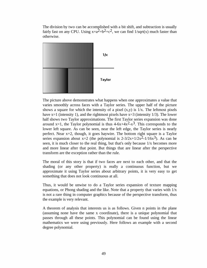
49

The division by two can be accomplished with a bit shift, and subtraction is usuallyfairly fast on any CPU. Using x=a2+b2+c2, we can find 1/sqrt(x) much faster thanotherwise.

The picture above demonstrates what happens when one approximates a value thatvaries smoothly across faces with a Taylor series. The upper half of the pictureshows a square for which the intensity of a pixel (x,y) is 1/x. The leftmost pixelshave x=1 (intensity 1), and the rightmost pixels have x=3 (intensity 1/3). The lowerhalf shows two Taylor approximations. The first Taylor series expansion was donearound x=1, the Taylor polynomial is thus 4-6x+4x2-x3. This corresponds to thelower left square. As can be seen, near the left edge, the Taylor series is nearlyperfect. Near x=2, though, it goes haywire. The bottom right square is a Taylorseries expansion about x=2 (the polynomial is 2-3/2x+1/2x2-1/16x3). As can beseen, it is much closer to the real thing, but that's only because 1/x becomes moreand more linear after that point. But things that are linear after the perspectivetransform are the exception rather than the rule.

The moral of this story is that if two faces are next to each other, and that theshading (or any other property) is really a continuous function, but weapproximate it using Taylor series about arbitrary points, it is very easy to getsomething that does not look continuous at all.

Thus, it would be unwise to do a Taylor series expansion of texture mappingequations, or Phong shading and the like. Note that a property that varies with 1/xis not a rare thing in computer graphics because of the perspective transform, thusthe example is very relevant.

A theorem of analysis that interests us is as follows. Given n points in the plane(assuming none have the same x coordinate), there is a unique polynomial thatpasses through all these points. This polynomial can be found using the linearmathematics we were using previously. Here follows an example with a seconddegree polynomial.

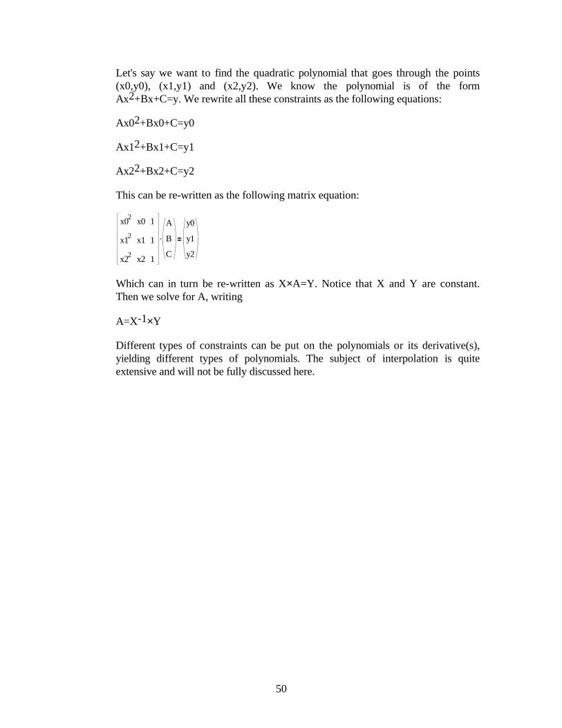
50

Let's say we want to find the quadratic polynomial that goes through the points(x0,y0), (x1,y1) and (x2,y2). We know the polynomial is of the formAx2+Bx+C=y. We rewrite all these constraints as the following equations:

Ax02+Bx0+C=y0

Ax12+Bx1+C=y1

Ax22+Bx2+C=y2

This can be re-written as the following matrix equation:

.

x02

x12

x22

x0

x1

x2

1

1

1

A

B

C

y0

y1

y2

Which can in turn be re-written as X×A=Y. Notice that X and Y are constant.Then we solve for A, writing

A=X-1×Y

Different types of constraints can be put on the polynomials or its derivative(s),yielding different types of polynomials. The subject of interpolation is quiteextensive and will not be fully discussed here.

51

Polynomial Splines

Introduction

In this section, I will have to assume a basic knowledge of calculus. Note that thetopic of spline is rather broad, hence only the basics will be covered here. For amore detailed discussion, one can see [5].

Sometimes we have many control points (10, for example) that we want to use togenerate an interpolating polynomial. However, we might not want to use a 10thdegree polynomial for several reasons. They're hard to evaluate. They'renumerically unstable. They tend to oscillate wildly between control points.

To resolve this, we make lower degree interpolating polynomials for each sectionof the curve. Typically, polynomials of degree 1 (lines), 2 (quadratics) or 3(cubics) are used. Polynomials of degree higher than 5 are unwieldy and alsosometimes exhibit undesirable behavior.

Basic splines

A spline will be defined by its type and a list of control points of the form {p1, p2,p3, ..., pn} where pi=(xi,yi) some point in 2d space. The type can be a simple linesegment joining each control points, or something more complex like a Catmull-Rom cubic spline. Note that a spline does not necessarily pass through allinterpolation points. It is even possible that a spline does not pass through any ofthe control points. We will examine such cases later.

We will start by an example spline of degree 1 that interpolates through all controlpoints. An example picture is shown below:

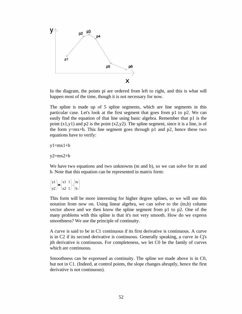
52

In the diagram, the points pi are ordered from left to right, and this is what willhappen most of the time, though it is not necessary for now.

The spline is made up of 5 spline segments, which are line segments in thisparticular case. Let's look at the first segment that goes from p1 to p2. We caneasily find the equation of that line using basic algebra. Remember that p1 is thepoint (x1,y1) and p2 is the point (x2,y2). The spline segment, since it is a line, is ofthe form y=mx+b. This line segment goes through p1 and p2, hence these twoequations have to verify:

y1=mx1+b

y2=mx2+b

We have two equations and two unknowns (m and b), so we can solve for m andb. Note that this equation can be represented in matrix form:

y1

y2.

x1

x2

1

1

m

b

This form will be more interesting for higher degree splines, so we will use thisnotation from now on. Using linear algebra, we can solve to the (m,b) columnvector above and we then know the spline segment from p1 to p2. One of themany problems with this spline is that it's not very smooth. How do we expresssmoothness? We use the principle of continuity.

A curve is said to be in C1 continuous if its first derivative is continuous. A curveis in C2 if its second derivative is continuous. Generally speaking, a curve in Cj'sjth derivative is continuous. For completeness, we let C0 be the family of curveswhich are continuous.

Smoothness can be expressed as continuity. The spline we made above is in C0,but not in C1. (Indeed, at control points, the slope changes abruptly, hence the firstderivative is not continuous).

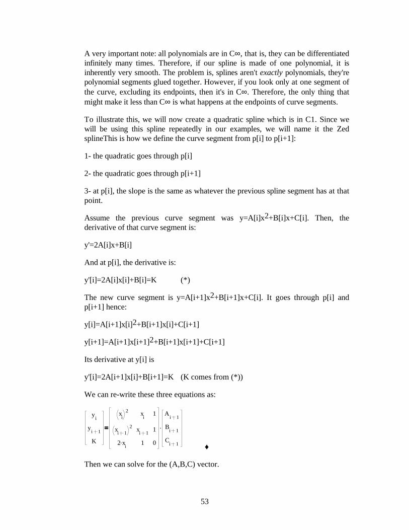
53

A very important note: all polynomials are in C∞, that is, they can be differentiatedinfinitely many times. Therefore, if our spline is made of one polynomial, it isinherently very smooth. The problem is, splines aren't exactly polynomials, they'repolynomial segments glued together. However, if you look only at one segment ofthe curve, excluding its endpoints, then it's in C∞. Therefore, the only thing thatmight make it less than C∞ is what happens at the endpoints of curve segments.

To illustrate this, we will now create a quadratic spline which is in C1. Since wewill be using this spline repeatedly in our examples, we will name it the ZedsplineThis is how we define the curve segment from p[i] to p[i+1]:

1- the quadratic goes through p[i]

2- the quadratic goes through p[i+1]

3- at p[i], the slope is the same as whatever the previous spline segment has at thatpoint.

Assume the previous curve segment was y=A[i]x 2+B[i]x+C[i]. Then, thederivative of that curve segment is:

y'=2A[i]x+B[i]

And at p[i], the derivative is:

y'[i]=2A[i]x[i]+B[i]=K (*)

The new curve segment is y=A[i+1]x2+B[i+1]x+C[i]. It goes through p[i] andp[i+1] hence:

y[i]=A[i+1]x[i] 2+B[i+1]x[i]+C[i+1]

y[i+1]=A[i+1]x[i+1] 2+B[i+1]x[i+1]+C[i+1]

Its derivative at y[i] is

y'[i]=2A[i+1]x[i]+B[i+1]=K (K comes from (*))

We can re-write these three equations as:

yi

yi 1

K

.

xi

2

xi 1

2

.2 xi

xi

xi 1

1

1

1

0

Ai 1

Bi 1

Ci 1 ♦

Then we can solve for the (A,B,C) vector.

54

There is still the question of generating the very first spline segment, since there isno such thing as "previous spline segment's slope at p[1]" (we'll have a hard timecomputing K). One solution is to let the first spline segment be a quadratic thatinterpolates through p[1], p[2] and p[3] exactly. Then the second curve segmentwill maintain the same slope as the first curve segment at p[2], and interpolatethrough p[2] and p[3].

Parametrized splines

As of now, our splines are functions, that is, they cannot curl backwards veryeasily. Infinite slopes are impossible. That and other things lead us to parametricsplines.

Right now, we have y as a function of x. We will now replace this with y afunction of t, and x a function of t. Then we plot all points (x,y) for some values oft and we get the desired spline. We use t as a variable name because it cansometimes be useful to think of the spline as an (x,y) point moving in time. Forexample, a spaceship's movement could possibly be described as(x,y,z)=(f(t),g(t),h(t)), a function of time for each coordinate. The key point here isthat this allows us to extend splines to any number of dimensions elegantly.

The control points are now of the form (x,y,t) or (x,y,z,t), depending on thenumber of dimensions we want. A parametric quadratic spline segment in 2d, forinstance, would be something of the form:

x=At2+Bt+C

y=At2+Bt+C

We just take each component individually and make it a spline as a function oftime. For example, if we have the control points (x0,y0,z0,t0) (x1,y1,z1,t1), ...,(xn,yn,zn,tn). Then, we look at x as a function of t, and make it a spline with thecontrol points (x0,t0), (x1,t1), (x2,t2), ..., (xn,tn). We do the same for y as a functionof t, with the control points (y0,t0), (y1,t1), ..., (yn,tn), and similarly for z as afunction of t.

Uniform splines

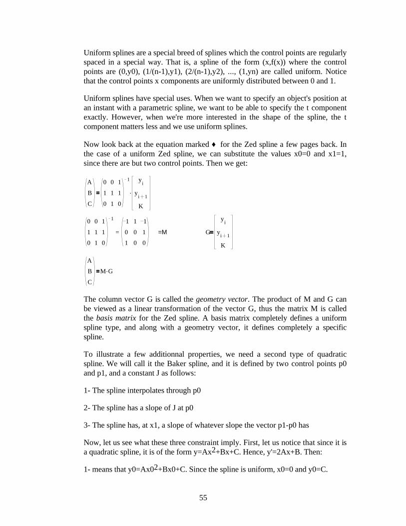
55

Uniform splines are a special breed of splines which the control points are regularlyspaced in a special way. That is, a spline of the form (x,f(x)) where the controlpoints are (0,y0), (1/(n-1),y1), (2/(n-1),y2), ..., (1,yn) are called uniform. Noticethat the control points x components are uniformly distributed between 0 and 1.

Uniform splines have special uses. When we want to specify an object's position atan instant with a parametric spline, we want to be able to specify the t componentexactly. However, when we're more interested in the shape of the spline, the tcomponent matters less and we use uniform splines.

Now look back at the equation marked ♦ for the Zed spline a few pages back. Inthe case of a uniform Zed spline, we can substitute the values x0=0 and x1=1,since there are but two control points. Then we get:

A

B

C

.

0

1

0

0

1

1

1

1

0

1 yi

yi 1

K

=

0

1

0

0

1

1

1

1

0

1 1

0

1

1

0

0

1

1

0

=M G

yi

yi 1

K

A

B

C

.M G

The column vector G is called the geometry vector. The product of M and G canbe viewed as a linear transformation of the vector G, thus the matrix M is calledthe basis matrix for the Zed spline. A basis matrix completely defines a uniformspline type, and along with a geometry vector, it defines completely a specificspline.

To illustrate a few additionnal properties, we need a second type of quadraticspline. We will call it the Baker spline, and it is defined by two control points p0and p1, and a constant J as follows:

1- The spline interpolates through p0

2- The spline has a slope of J at p0

3- The spline has, at x1, a slope of whatever slope the vector p1-p0 has

Now, let us see what these three constraint imply. First, let us notice that since it isa quadratic spline, it is of the form y=Ax2+Bx+C. Hence, y'=2Ax+B. Then:

1- means that y0=Ax02+Bx0+C. Since the spline is uniform, x0=0 and y0=C.

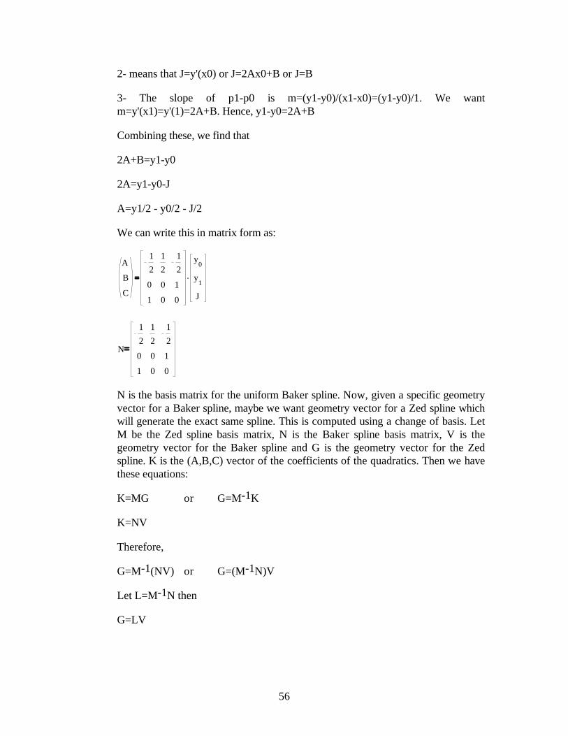
56

2- means that J=y'(x0) or J=2Ax0+B or J=B

3- The slope of p1-p0 is m=(y1-y0)/(x1-x0)=(y1-y0)/1. We wantm=y'(x1)=y'(1)=2A+B. Hence, y1-y0=2A+B

Combining these, we find that

2A+B=y1-y0

2A=y1-y0-J

A=y1/2 - y0/2 - J/2

We can write this in matrix form as:

A

B

C

.

1

2

0

1

1

2

0

0

1

2

1

0

y0

y1

J

N

1

2

0

1

1

2

0

0

1

2

1

0

N is the basis matrix for the uniform Baker spline. Now, given a specific geometryvector for a Baker spline, maybe we want geometry vector for a Zed spline whichwill generate the exact same spline. This is computed using a change of basis. LetM be the Zed spline basis matrix, N is the Baker spline basis matrix, V is thegeometry vector for the Baker spline and G is the geometry vector for the Zedspline. K is the (A,B,C) vector of the coefficients of the quadratics. Then we havethese equations:

K=MG or G=M-1K

K=NV

Therefore,

G=M-1(NV) or G=(M-1N)V

Let L=M-1N then

G=LV

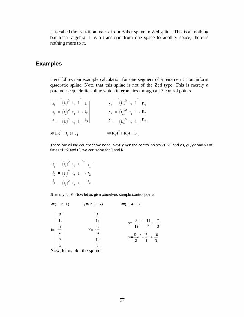
57

L is called the transition matrix from Baker spline to Zed spline. This is all nothingbut linear algebra. L is a transform from one space to another space, there isnothing more to it.

Examples

Here follows an example calculation for one segment of a parametric nonuniformquadratic spline. Note that this spline is not of the Zed type. This is merely aparametric quadratic spline which interpolates through all 3 control points.

x1

x2

x3

.

t12

t22

t32

t1

t2

t3

1

1

1

J1

J2

J3

y1

y2

y3

.

t12

t22

t32

t1

t2

t3

1

1

1

K1

K2

K3

x .J1 t2 .J2 t J3 y .K1 t

2 .K2 t K3

These are all the equations we need. Next, given the control points x1, x2 and x3, y1, y2 and y3 at times t1, t2 and t3, we can solve for J and K.

J1

J2

J3

.

t12

t22

t32

t1

t2

t3

1

1

1

1

x1

x2

x3

Similarly for K. Now let us give ourselves sample control points:

x ( )0 2 1 y ( )2 3 5 t ( )1 4 5

x .5

12t2 .11

4t

7

3J

5

12

11

4

7

3

K

5

12

7

4

10

3

y .5

12t2 .7

4t

10

3

Now, let us plot the spline:

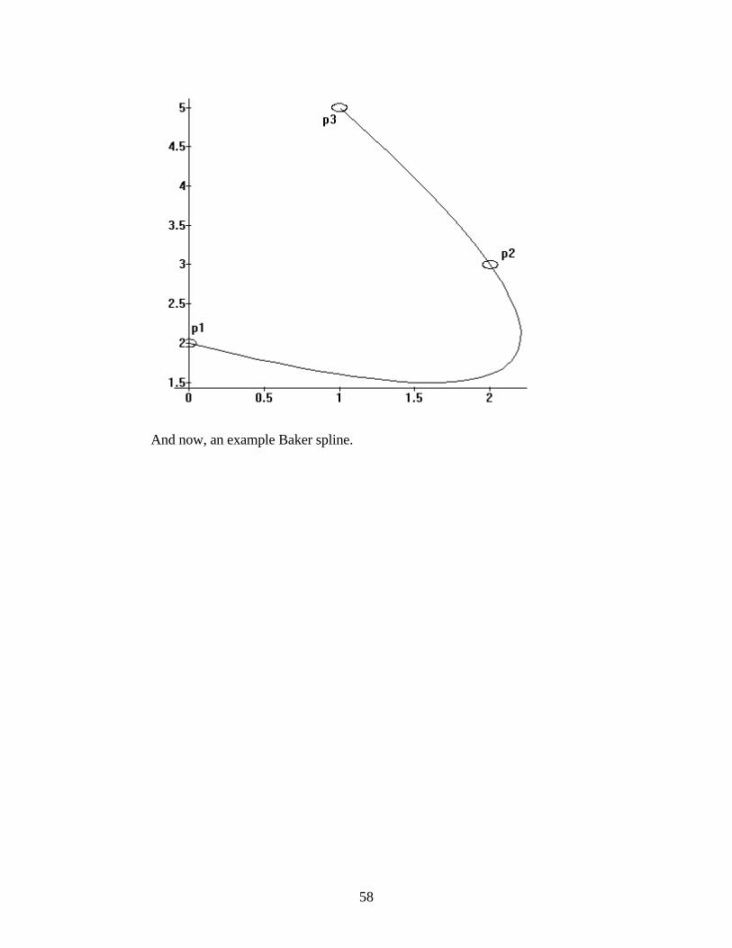
58

And now, an example Baker spline.

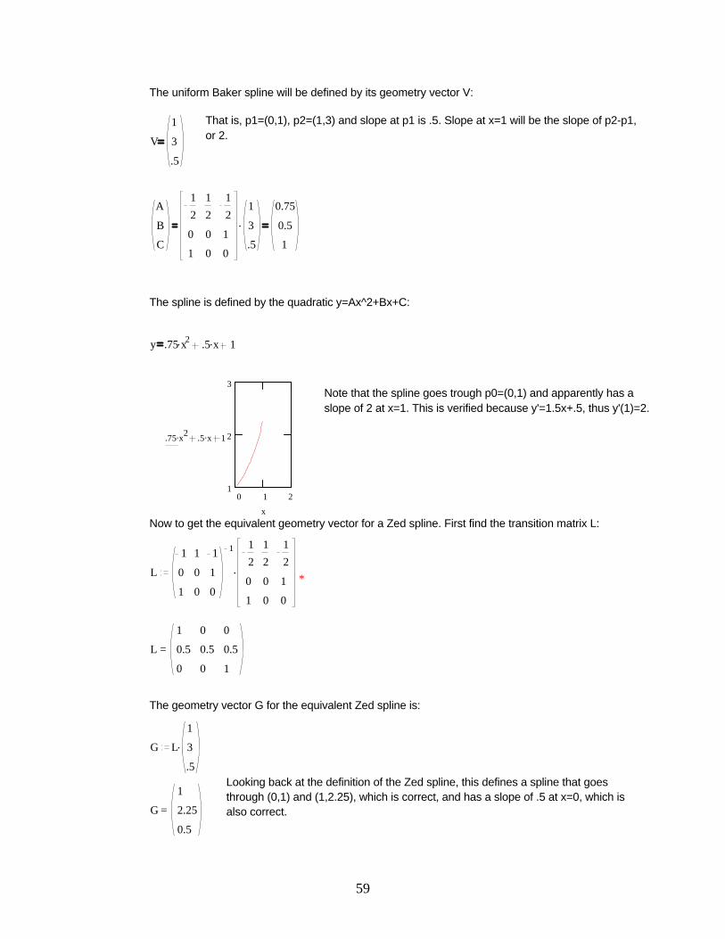
59

The uniform Baker spline will be defined by its geometry vector V:

That is, p1=(0,1), p2=(1,3) and slope at p1 is .5. Slope at x=1 will be the slope of p2-p1, or 2.V

1

3

.5

A

B

C

.

1

2

0

1

1

2

0

0

1

2

1

0

1

3

.5

0.75

0.5

1

The spline is defined by the quadratic y=Ax^2+Bx+C:

y ..75x2 ..5 x 1

0 1 21

2

3

..75 x2 ..5 x 1

x

Note that the spline goes trough p0=(0,1) and apparently has a slope of 2 at x=1. This is verified because y'=1.5x+.5, thus y'(1)=2.

Now to get the equivalent geometry vector for a Zed spline. First find the transition matrix L:

*L .

1

0

1

1

0

0

1

1

0

1 1

2

0

1

1

2

0

0

1

2

1

0

=L

1

0.5

0

0

0.5

0

0

0.5

1

The geometry vector G for the equivalent Zed spline is:

G .L

1

3

.5Looking back at the definition of the Zed spline, this defines a spline that goes through (0,1) and (1,2.25), which is correct, and has a slope of .5 at x=0, which is also correct.=G

1

2.25

0.5

60

Frequently used uniform cubic splines

A certain number of uniform cubic splines very useful for various reasons, mostlymodelling curves. Some of these will be described here. The Hermite spline isdefined by four two control points P1 and P2 and 2 slopes vector S1 and S2.Bézier splines are defined by 4 control points P1 through P4 and uniformnonrational B-splines are also defined by 4 control points, with differentconstraints however.

A few general notes before we dive into the main material. These splines arecubics, hence they are of the form y=Ax3+Bx2+Cx+D and the derivative of such acubic is y'=3Ax2+2Bx+C. Often, constraints will be put on y(x) or y'(x) for somex, which will then be used to figure out the basis matrix for the spline.

Hermite splines

The hermite spline is defined by two control points P1 and P2, and two slopes s1and s2 as follows:

1- The spline interpolates through P1

2- The spline interpolates through P2

3- The slope at P1 is s1

4- The slope at P2 is s2

Since the spline is uniform, P1=(0,y1) and P2=(1,y2). The geometry vector G is(y1,y2,s1,s2). We re-write the four constraints using that:

1- y1=D

2- y2=A+B+C+D

3- s1=C

4- s2=3A+2B+C

We re-write in matrix form and solve for (A,B,C,D):

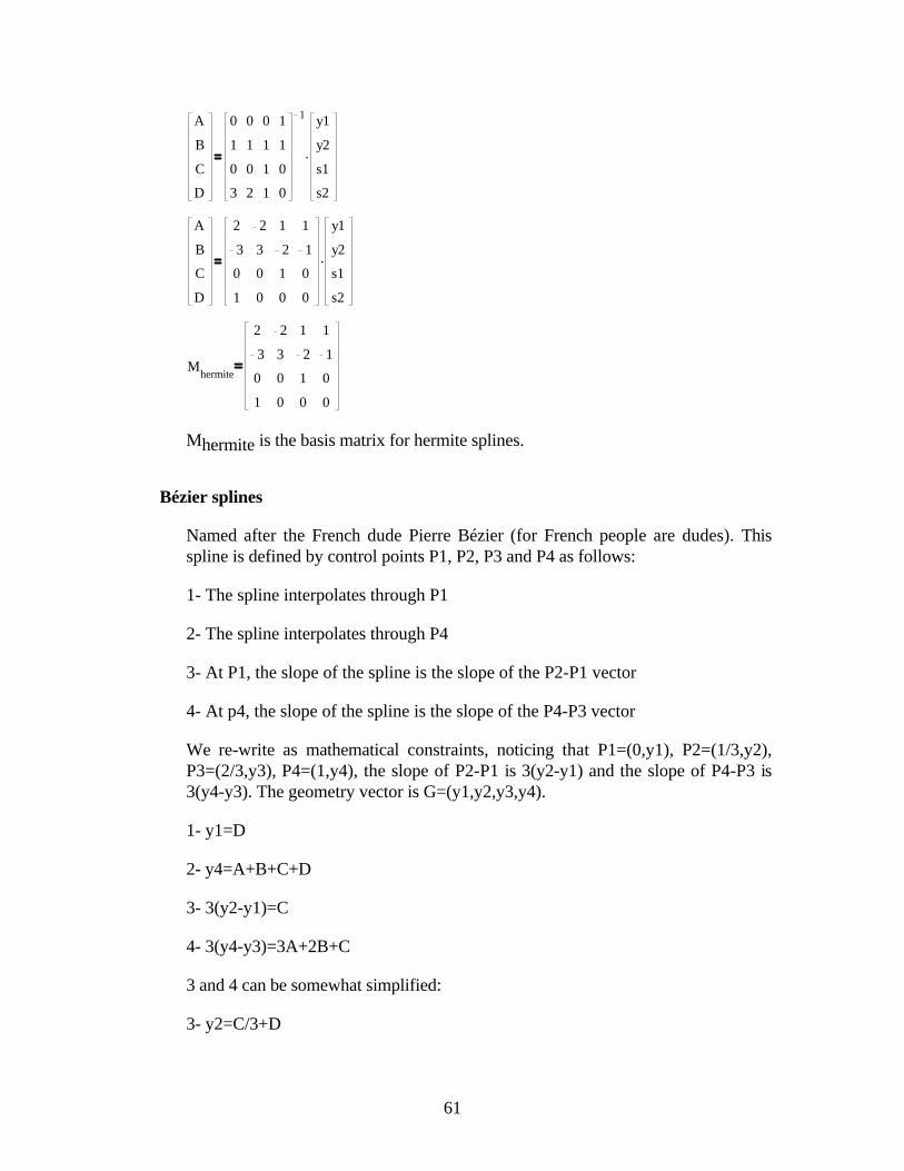
61

A

B

C

D

.

0

1

0

3

0

1

0

2

0

1

1

1

1

1

0

0

1 y1

y2

s1

s2

A

B

C

D

.

2

3

0

1

2

3

0

0

1

2

1

0

1

1

0

0

y1

y2

s1

s2

Mhermite

2

3

0

1

2

3

0

0

1

2

1

0

1

1

0

0

Mhermite is the basis matrix for hermite splines.

Bézier splines

Named after the French dude Pierre Bézier (for French people are dudes). Thisspline is defined by control points P1, P2, P3 and P4 as follows:

1- The spline interpolates through P1

2- The spline interpolates through P4

3- At P1, the slope of the spline is the slope of the P2-P1 vector

4- At p4, the slope of the spline is the slope of the P4-P3 vector

We re-write as mathematical constraints, noticing that P1=(0,y1), P2=(1/3,y2),P3=(2/3,y3), P4=(1,y4), the slope of P2-P1 is 3(y2-y1) and the slope of P4-P3 is3(y4-y3). The geometry vector is G=(y1,y2,y3,y4).

1- y1=D

2- y4=A+B+C+D

3- 3(y2-y1)=C

4- 3(y4-y3)=3A+2B+C

3 and 4 can be somewhat simplified:

3- y2=C/3+D

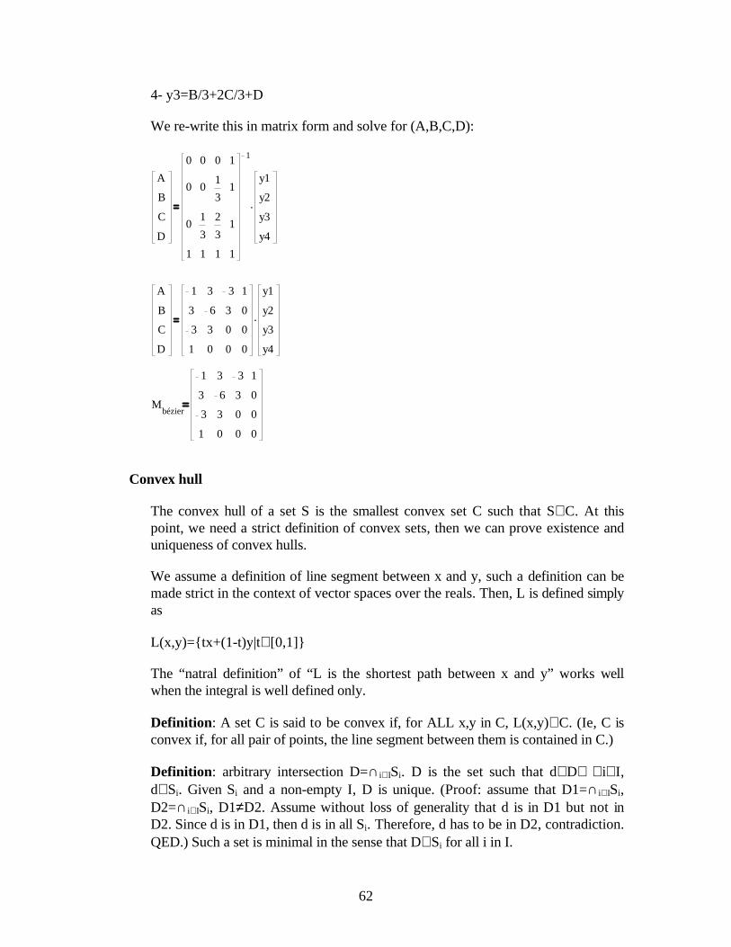
62

4- y3=B/3+2C/3+D

We re-write this in matrix form and solve for (A,B,C,D):

A

B

C

D

.

0

0

0

1

0

0

1

3

1

0

1

3

2

3

1

1

1

1

1

1

y1

y2

y3

y4

A

B

C

D

.

1

3

3

1

3

6

3

0

3

3

0

0

1

0

0

0

y1

y2

y3

y4

Mbézier

1

3

3

1

3

6

3

0

3

3

0

0

1

0

0

0

Convex hull

The convex hull of a set S is the smallest convex set C such that S⊆ C. At thispoint, we need a strict definition of convex sets, then we can prove existence anduniqueness of convex hulls.

We assume a definition of line segment between x and y, such a definition can bemade strict in the context of vector spaces over the reals. Then, L is defined simplyas

L(x,y)={tx+(1-t)y|t∈ [0,1]}

The “natral definition” of “L is the shortest path between x and y” works wellwhen the integral is well defined only.

Definition : A set C is said to be convex if, for ALL x,y in C, L(x,y)⊆ C. (Ie, C isconvex if, for all pair of points, the line segment between them is contained in C.)

Definition : arbitrary intersection D=∩ i∈ ISi. D is the set such that d∈ D⇔∀ i∈ I,d∈ Si. Given Si and a non-empty I, D is unique. (Proof: assume that D1=∩ i∈ ISi,D2=∩ i∈ ISi, D1≠D2. Assume without loss of generality that d is in D1 but not inD2. Since d is in D1, then d is in all Si. Therefore, d has to be in D2, contradiction.QED.) Such a set is minimal in the sense that D⊆ Si for all i in I.

63

Definition : Convex hull. First assume the universe U is convex (this is true forRn). Then, the convex hull C of an arbitrary set S is defined as ∩Cα, whereK={C α} is the set of all convex supersets of S. Since S is in U and U is convex, Uis an element of K, thus the intersection exists and is unique. It is also minimal. Allwe have to prove is that C is convex. But this is trivial, as we are about to show.Take an arbitrary pair of points x, y in C. We have to prove that L(x,y) is a subsetof C. Since x and y are in C, x and y have to be in Cα for all α. Since Cα is convex,this means that L(x,y) is in Cα for all α. Therefore, L(x,y) is in C. This is true forany x,y in C, thus C is convex.

As an example, a triangle is its own convex hull. For a concave polygon, theconvex hull is the smallest convex polygon that completely includes the concavepolygon.

Now on to convex sums. A convex sum is a weighted sum ∑1≤i≤nwiyi such that∑1≤i≤nwiyi=1 and wi is non-negative. A convex sum is so called because the resultingsum is in the convex hull of its control points yi, as we are about to prove. We willhere use a proof by induction. Let us first articulate the proposition we are aboutto prove.

Pi=“The sum Si =∑1≤j≤iwjyj where the weights wj are positive and sum to 1 lieswithin the convex hull of the control points yj.”

P1 translates into w1y1, where w1 is positive and w1=1, is in the convex hull of y1,which trivially true.

The next step is to demonstrate that Pi⇒ Pi+1. Now let us examine Pi+1.∑1≤j≤i+1wjyj=∑1≤j≤iwjyj+wi+1yi+1. Let K=∑1≤j≤iwj. We know that K<1 since allweights are positive and add up to 1. We can scale up Si by 1/K (call that Q).Then, by hypothesis of Pi, Q is in the convex hull of the y1 through yi. However,Si+1=KQ+wi+1yi+1 and K+ wi+1=1. Thus Si+1 is on the line between Q and yi+1. Sinceboth Q and yi+1 are in the convex hull of y1 through yi+1, the line between Q and yi+1

is in the convex hull. Thus Si+1 is in the convex hull. By induction, Pi is true for alli, which completes the proof.

Bernstein polynomials

The nth degree Bernstein polynomial, Bn(x) is defined by n+1 control points y0,y1, y2, ..., yn as follows:

Bn(x)=∑0≤i≤nC(i,n)xi(1-x)n-iyi where C(i,n)=n!/[i!(n-i)!]

n! is the factorial of n, is 1×2×3×4×...×n. As an example, 6!=720. As per thedefinition above, C(3,5), for example, would be 5!/(3!2!)=10.

64

At this point in time, it is useful to view the spline as a weighted sum of its controlpoints. Looking at Bn(x) as above, we can see that for a fixed x, we are in effecttaking a weighted sum of the yi’s: ∑0≤i≤n wiyi. Let us now examine the weights.

A weight wi=C(i,n)xi(1-x)n-i as above can be interpreted probabilistically using thebinomial distribution. If we are repeating an experiment n (independant) times,each time with probability of success x, then wi is the probability of the experimentsucceding exactly i times. Then, it becomes obvious that ∑0≤i≤n wi =1 (the sum issimply the sum of the probabilities of all possible outcomes, which has to be one).

Going back to Bn(x), we can now say that the Bernstein polynomial is a convexsum of its control points. A convex sum is when the sum of the weights is one adeach weight is positive (as is the case here). It is so called because then the resultwill be in the convex hull of the control points. Of particular interest to us is theB3(x) polynomial. It can be written down as follows:

B3(x) =y0(1-x)3+y13x(1-x)2+y23x2(1-x)+y3x3

=y0(1-3x+3x2-x3)+y1(3x-6x2+3x3)+y2(3x2-3x3)+y3x3

=x3(-y0+3y1-3y2+y3)+x2(3y0-6y1+3y2)+x(-3y0+3y1)+y0.

It is obvious from this last form that we have just found an equivalent definition tothe Bézier spline. With the work we have just accomplished, we havedemonstrated that a Bézier spline lies within the convex hull of its control points,which is an important property, as we will see later.

Uniform nonrational B-spline

The uniform nonrational B-spline is defined as a cubic polynomial spline which hasC2 continuity everywhere even when several B-spline segments are put insequence. The term nonrational refers to the fact that we are dealing here with aconventional polynomial, as opposed to a quotient of polynomials. A rationalspline is defined by the quotient of two polynomials.

The B-spline is defined by 4 control points P1, P2, P3, P4. However, let usexamine exactly how we should use these to make certain that consecutive B-splines are C0, C1 and C2 continuous. That is, say we have 6 points P0, P1, P2,P3, P4 and P5. Then, the B-spline defined by P1, P2, P3 and P4 is the one we areinterested in, let's call it segment S2. However, there is a spline segment defined byP0, P1, P2, P3, which we will call S1. We want S1 and S2 to have C0, C1 and C2continuity at their joint. Furthermore, there is a spline defined by P2, P3, P4 andP5, which we name S3, and we want S2 and S3 to have C0, C1 and C2 continuityat their joint.

This section in progress, I can't find a justification for the B-spline basis matrix.

65

Catmull-Rom splines: a non-uniform type of spline

This spline type is defined as follows (given four control points P0 through P3

(x0,y0), (x1,y1), (x2,y2) and (x3,y3), xi are increasing):

1- The spline interpolates through (x1,y1).

2- The spline interpolates through (x2,y2).

3- The spline’s slope at x0 (the second control point) is whatever slope the linefrom the first to the third control point is.

4- The spline’s slope at x1 (the third control point) is whatever slope the line fromthe second to the fourth control point is.

The spline segment thus defined is for the [x1,x2] segment. If a similar spline isdefined with the control points P1, P2, P3, P4, then they will join at P2 and their firstderivative will agree, giving it a smooth appearance. Writing the restrictionsexpressly in equation form, we get:

1- y1=Ax13+Bx1

2+Cx1+D.

2- y2=Ax23+Bx2

2+Cx2+D.

3- y’(x1)=3Ax12+2Bx1+C=(y2-y0)/(x2-x0).

4- y’(x2)=3Ax22+2Bx2+C=(y3-y1)/(x3-x1).

66

Rendering

Introduction

Rendering is the phase where we do the actual drawing. There is a generaltendency to download this particular task to a slave graphics processor and leavethe CPU to do better things. However, it will always be useful for everyone tohave a general understanding of how things work. And also likely is the fact thatwe're going to need software renderers for a while more. And one last fact is thatpeople have to write the software for the slave processor.

We will first study the drawing of a point, which will be used to draw otherprimitives. Then we will study lines and polygons. Curved surfaces can also besupported but will not be discussed. The curved primitive that tend to be faster indrawing are conics and polynomials. However, some other forms of curvedprimitives definitions are often preferred, mainly splines.

The point

A geometric point is a 0 dimensional object. It could also be defined very strictlywith neighborhoods and somesuch. However, this is not particularly useful to thecomputer graphics specialist. One thing that we must remember, though, is that itis impossible to display a point on any medium. Quite simply, a point has a size ofzero, no matter if the definition of size is length, area or volume. It cannot be seenunder any magnification.

What the computer graphics expert usually refers to as the point is the smallestentity that can be displayed on the display device. These are not necessarilycircular or rectangular things - and more often than not, they are slightly blurred.

We will refer to this point as a pixel. We will also need to make a few basicassumptions. Generally speaking, pixels are of an arbitrary shape (oftenrectangular-like), and are aligned in a very structured way on the display device.Note that some devices do not use this method of displaying things, these arecommonly referred to as vector devices. There was an old Star Wars (trademark ofLucasArts I believe) game made with one of these.

67

We will also very much like pixel to be aligned in a cartesian plane like manner.We generally assign pixels integer position, and what's not exactly on a pixel has anoninteger position. But what is the position of the pixel? That's another entirelyarbitrary matter. Generally speaking, we might want to simplify the pixel's locationto its centroid. Also, there is the problem of axis orientation. For a combination ofarbitrary and historical reasons, the screen coordinates origin is very usuallycentered on the upper left corner and goes positively down and right in hardware.Operating sometimes hide that from the user application and use a coordinatesystem centered on the lower left corner, and go positively up and right, just likethe usual cartesian plane.

The way that pixels are stored internally is also of importance. Generally speaking,each pixel is assigned a color, and the number of colors available per pixel isdefined by the number of bits allocated to each pixel. For instance, if each pixel has6 bits of color data to it, then each pixel can be one of 64 colors. When a "strange"number of bits per pixel is used, it often happens that the bits are spread in a lessintuitive way. For example, in the 6 bit case, instead of using one byte per pixeland wasting 2 bits per pixel, the system will likely store bit 0 of all pixels, then bit 1of all pixels, then bit 2 of all pixels, and so on. This is called a bit-planearrangement.

If the number of bits per pixel is closer to 8, 16, 24 or 32, then some systems willallow what is generally referred to as a linear arrangement of pixels. For example,if 8 bits are allocated per pixel, then one byte corresponds to one pixel.

It is generally accepted that with 24 bits per pixel, the human eye cannot see thedifference between two very similar shades of the same color. (High end platformstoday use 16 bits per component, including a so-called alpha channel, for apossible total of 64 bits, but this is to minimize roundoff when combining severalimages together, for instance.) However, 24 bits per pixel is roughly 16 millions ofcolors. Thus, when using a mere 6 or 8 bits per pixel, sacrifices must be made.

One way that the industry has found is to make a look-up table. As an example,each pixel is assigned a value from 0 to 255 (for 8 bits), and the hardware is givena lookup table of 256 color entries. Each color entry can contain a 16 or 24 bitcolor for example. Then, the hardware automatically substitute the proper entry inthe table for each pixel when it has to display them. The lookup table is oftenreferred to as the palette or color map.

68

At any rate, eventually one needs a way of identifying colors, either to select thecolor map colors, or in the case of a 24 or 32 bits system, select the pixel color.There are several ways of doing this. Two of the most popular means are RGBcolors and HSV colors. RGB is an acronym for red, green and blue. Colors arespecified by their red, green and blue contents. It is interesting to note that displaysusually do not use red, green and blue, but colors that are close to these. Thecolors actually used by the displays were selected to allow for a broader range ofcolors.

Another popular means of selecting a color is with HSV values. This is anotheracronym that stands for Hue, Saturation and Brightness (isn't that last oneobvious?) This model is more intuitive than the RGB model for most people. Othermodels include the CMY (Cyan, Magenta and Yellow) and YIQ (Luminance andChromaticity) models.

Writing to a specific pixels usually involves finding an address and then putting avalue in it. Since memory is usually mapped in a one dimensional fashion, devicepixels are mapped in an arbitrary way to memory. Usually, finding a memorylocation for a pixel involves a multiplication. However, multiplications are typicallyexpensive, thus we might want to look into that a bit further. Let us assume a800x600 display, with 8 bits per pixel and linear mapping.

A base address A has to be given for the top-leftmost pixel (assuming origin is attop-left). Then, the first row of 800 pixels would be the next 800 bytes. Then nextrow of 800 pixels would follow and so on. Generally speaking, pixel (x,y) for aninteger x and y can be found at memory location A+x+y*800. Note that somesystems will want to pad each row with a few bytes sometimes.

Multiplying once per pixel write is a bit expensive. There are several workarounds.The first one is straightforward but hardware dependant. The second one assumesthat we access pixels in a coherent way (not totally random).

If the width of the display device in pixels is known in advance, the multiplicationcan be removed the following way. Say the pixel to be addressed is at memorylocation A+x+y*800. 800 is 512+256+32, thus we have A+x+y(512+256+32) =A+x+512y+256y+32y. However, 512=29, 256=28 and 32=25 Thus, the pixelmemory location is A+x+29y+28y+25y. Note that a multiplication by a power oftwo can be optimized out with left shifts, which are typically much faster thanmultiplications. Let a<<b denote a shifted left by b bits, then the memory locationof the pixel can be expressed as:

A+x+y<<9+y<<8+y<<5.

Similar decompositions in powers of two of various scalars can be found. Theproblem with this is that it requires the scalar (display device width in pixels) to behard-coded in the program.

69

Another way of accessing pixels is by exploiting coherence. If we plane to accessall the pixels on a given scanline, starting from left to right, then the following istrue.

Pixel at memory location A+y*width is the leftmost pixel on the scanline. Thesecond leftmost value is the above value plus one. The third one can be found byadding one again, and so forth. Thus, accessing pixels that are adjacent on ascanline can be done in one add per pixel only.

Accessing pixels that are on the same column is similar, except that <width> isadded each time to the memory location.

Lines

There are a number of ways to draw lines. Generally, they all boil down to thesame basic ideas, and have roughly comparable speeds. The algorithm presentedhere is the one I felt had the best mixture of simplicity, efficiency and small size. Ithas the disadvantage of being less exact than some other algorithms for lines ofrational slopes. We will first start with special cases, then move to more generalcases.

The simplest lines to draw are the horizontal and vertical ones. As can be imaginedeasily by the reader from the last section, we start with the topmost or leftmostpixel, draw it, then either add 1 or <width> to memory location and draw the nextpixel. And so on, for the length of the line.

The next step up is an angled line. If the line is not vertical nor horizontal, then itcan be expressed as y=mx+b or x=ny+c, with n=1/m and c=-b/m, whichever ispreferred. The representation one has to use is whichever of the two has thesmallest m or n. This is to ensure that there are no large gaps between the pixels ofa line. Afterwards, we initialize (x0,y0) to be one endpoint of the line. If we chosey=mx+b, we should be using the leftmost endpoint for (x0,y0). We draw (x0,y0),then increment x, and add m to y. Then we draw the new point. The extension tothe x=ny+c form is left to the reader.

Notice that the previous paragraph is simply an application of forward differencingstudied previously. The witty reader will easily imagine the extension of this tohigher degree polynomials. It is also possible to extend incremental algorithms tocircles and ellipses, amongst others, but we will not go into this.

In some applications, such as polygon drawing, one of either y=mx+b or x=ny+cwill be preferred even if the slope is greater than 1.

70

Note that the topic of line drawing can be extended much more than this. Anti-aliased lines, line width and patterns, endpoint shape are all topics that we will notcover.

This algorithm has the nice property of being a special case of forwarddifferencing. It's also fast and has no comparisons in the so-called inner loop.(Comparisons have a tendency to flush prefetch queues in CPU's, which results inrelatively long delays in the inner loop).

However it has the disadvantage of accumulating roundoff error at each new pixel.This should not be a problem in general, but when utmost precision is needed, analternate algorithm which does not accumulate error might be considered.

The algorithm works without any error accumulation (the only error is theroundoff to the nearest pixel). The idea is as follows. We first observe that theslope m is a rational of the form a/b. Let's assume m is positive and less than 1. Wecan make a special case for each of the 8 octants such that this is true.

Next, let's assume y0 is of the form N+c/b, where c is some integer between 0 andb. Then, when adding the slope to the current y, we get N+(c+a)/b. However, nowwe need to check whether c+a is more than b. If it is, then we rewrite as:N+(c+a)/b=N+(c+a-b+b)/b=N+1+(c+a-b)/b. This means that whenever c+a ismore than b, we subtract b from it and add 1 to N. The pixel coordinate in y thatwe actually draw is N. (This implies that we're truncating y. If we want to roundoff rather, we can add 0.5 to the original y0, which will have the net effect ofrounding to the closest integer. The denominator can be doubled to avoid roundoffin the .5). Pseudocode for this follows (integer endpoints are assumed, this can begeneralized to rational endpoints of course).

Let (x0,y0) and (x1,y1) be the endpoints of the line segment, suchthat (x1,y1) is in the first octant relative to (x0,y0).Let a=2*(y1-y0)Let b=2*(x1-x0)Let N=y0Let c=(x1-x0)

for x varying from x0 to x1 by steps of one, doputpixel(x,N)add a to cif c>=b then

subtract b from cadd 1 to N

end ifend for

Polygon drawing

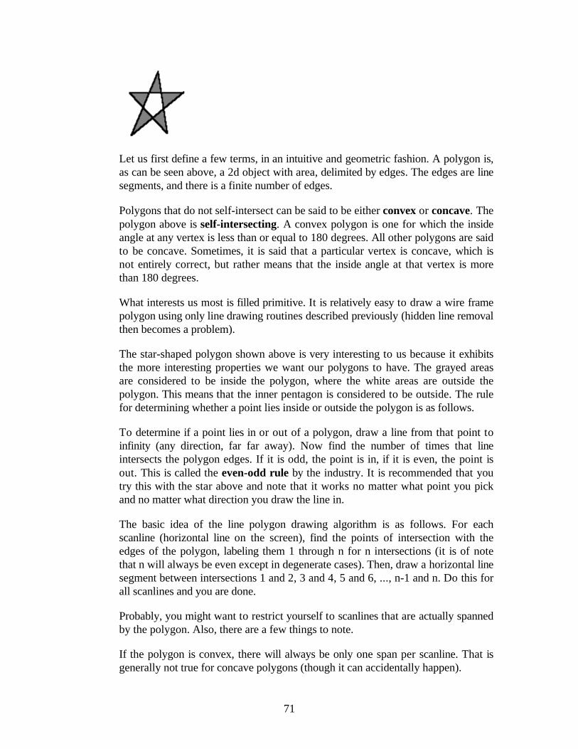
71

Let us first define a few terms, in an intuitive and geometric fashion. A polygon is,as can be seen above, a 2d object with area, delimited by edges. The edges are linesegments, and there is a finite number of edges.

Polygons that do not self-intersect can be said to be either convex or concave. Thepolygon above is self-intersecting. A convex polygon is one for which the insideangle at any vertex is less than or equal to 180 degrees. All other polygons are saidto be concave. Sometimes, it is said that a particular vertex is concave, which isnot entirely correct, but rather means that the inside angle at that vertex is morethan 180 degrees.

What interests us most is filled primitive. It is relatively easy to draw a wire framepolygon using only line drawing routines described previously (hidden line removalthen becomes a problem).

The star-shaped polygon shown above is very interesting to us because it exhibitsthe more interesting properties we want our polygons to have. The grayed areasare considered to be inside the polygon, where the white areas are outside thepolygon. This means that the inner pentagon is considered to be outside. The rulefor determining whether a point lies inside or outside the polygon is as follows.

To determine if a point lies in or out of a polygon, draw a line from that point toinfinity (any direction, far far away). Now find the number of times that lineintersects the polygon edges. If it is odd, the point is in, if it is even, the point isout. This is called the even-odd rule by the industry. It is recommended that youtry this with the star above and note that it works no matter what point you pickand no matter what direction you draw the line in.

The basic idea of the line polygon drawing algorithm is as follows. For eachscanline (horizontal line on the screen), find the points of intersection with theedges of the polygon, labeling them 1 through n for n intersections (it is of notethat n will always be even except in degenerate cases). Then, draw a horizontal linesegment between intersections 1 and 2, 3 and 4, 5 and 6, ..., n-1 and n. Do this forall scanlines and you are done.

Probably, you might want to restrict yourself to scanlines that are actually spannedby the polygon. Also, there are a few things to note.

If the polygon is convex, there will always be only one span per scanline. That isgenerally not true for concave polygons (though it can accidentally happen).

72

Here is pseudocode for a polygon filling algorithm.

Let an edge be denoted (x0,y0)-(x1,y1), where y0 ≤y1. Edges alsohave a "current x" value, denoted cx. Initialize cx to x0. Oneshould also compute the slope of all edges, denoted s, which is(x1-x0)/(y1-y0) (we are using the x=ny+c representation).Let IET be the inactive edge table, initially containing all edgesLet AET be the active edge table, initially empty

Sort the IET's edges by increasing values of y0Let the initial scanline number be the y0 of the first edge in theIET

RepeatWhile scanline ≥y0 of the topmost edge in the IET

Move topmost edge from IET to AETEnd while

(*) Sort AET in increasing values of cx

For every edge in the AETIf edge's y1 ≥scanline, then remove edge from AETElse add the slope "s" to "cx".

End for

For each pair of edge in the AETDraw a horizontal segment on current scanline betweencolumn "cx0" and "cx1", where "cx0" is the "cx" valuefor the first edge in the pair and "cx1" is the "cx"value for the second edge in the pair

End forUntil the AET is empty

It is of note that the line marked by (*) can be optimized out. If the polygon is notself-intersecting, we just need to make sure the AET is properly sorted when weinsert a new edge into it.

It should be noted that edges that are parallel to the scanline should not be put inthe IET. You might also need to clip the polygon to the viewport, which can beadded to the polygon blitting code.

73

Visible surface determination

Introduction

One of the problems we have yet to address, when several objects project to thesame area on screen, how do you decide which gets displayed. Intuitively, theclosest object should be the one to be displayed. Unfortunately, this definition isvery hard to handle. We will usually say that the object to be displayed will be theone with the smallest z value in eye space, which is a bit easier to work with. Acorollary of this is that objects with the largest 1/z value get displayed, this latterobservation has applications which will be explained later.

Visible surface determination can be done in a number of ways, each has itsadvantages, disadvantages and applications. Hidden line removal is used when wireframes are generated. This might be useful for a vector display, but will not becovered in here. When dealing with filled primitives, there are several classes ofvisible surface determination. There is also the question of object precision, deviceprecision, and more, these topics will not be discussed here.

Perhaps the most intuitive visible surface determination algorithm is the so-called"painter's algorithm", which works the same way a painter does. Namely, it drawsobjects that are further away first, then draws objects that are closer. Theadvantage of this is it's simple. The disadvantages are that it writes several times tosome areas of the display device, and also that some objects cannot be orderedcorrectly.

The painter's algorithm can be generalized into the depth-sorting algorithm, whichsort the primitives from back to front and then draw. The depth sorting algorithmalso resolves cases that painter's algorithm does not.

Another algorithm is space partitioning trees such as BSP (binary space partitions)trees. The advantage of this algorithm is to generate a correct ordering of theprimitives quickly and correctly no matter where the viewer is. The disadvantage isthat it is hard to add any polygons to a scene thus rendered, or to deform it in anonlinear way. Approximations can be made.

74

Yet another way of doing visible surface determination is the class of algorithmsgenerally referred to as "scan-line algorithms". These algorithms, thoughsomewhat slower than depth sorting, have the advantage of drawing to each andevery pixel of the display device once and only once. Thus there is no need to clearthe display in the first place, and pixels are not written to needlessly. Incidentally,this algorithm is very useful for display devices where it is impossible or difficult toerase or rewrite to pixels, such as printers. The disadvantages are that it's slightlyslower, and usually quite more messy to code than a depth sorting algorithm. Also,visible surface determination becomes an integral part of the polygon drawingroutine in most cases, making it hard to download the polygon drawing code tosome hardware, or to make several versions of polygon drawing code for differentdrawing modes.

A very popular way of doing visible surface determination is called z-buffering.This works by storing the z value whatever occupies a pixel for each pixel. Thisway, one can add new primitives to a scene, visible surface determination is just acompare away. Incidentally, it is usually much more efficient to use 1/z values thanit is to use z values, since 1/z varies linearly but z does not.

Another algorithm worth mentioning is the Weiler-Atherton algorithm, which clipsprimitives so that they do not intersect before drawing, and Warnock's algorithm,which recursively subdivides the display area until it can trivially determine whichprimitive to draw. These algorithms are fairly slow.

An optimization that can be made to any visible surface determination algorithm isback-face removal or back-face culling. This is based on the observation that facesthat are facing away from the observer

As of now, the only algorithms discussed will be the depth sort and painter'salgorithm, along with z buffering and back-face culling..

Back-face culling

Back-face culling exploits the observation that a face in a closed polyhedronalways has two sides. One faces inside, and can never be seen by an observeroutside the polyhedron (rather obviously since the polyhedron is closed), the otherfaces outside and can be seen. However, if it is determined that the side facing theeye is the inside of the face, that face will assuredly not be seen, because it isimpossible to see a face from the inside.

75

The side that faces the eye can be determined easily with dot product. Take avector V from the eye to any point within the polygon (for example, from the eyeto a vertex). Let A be the normal of the polygon, assuming that A points outwardsof the polyhedron. Then, compute V•A. If it is positive, the inside of the face istowards the camera, do not display or transform the face. If it is negative, the faceis facing the camera and might be seen (though this is not guaranteed).

Back-face culling is generally not sufficient for visible surface determination. It ismerely used to remove faces that assuredly cannot be seen. However, it will donothing for faces that are only obscured by faces that are closer. Also, back-faceremoval assumes that the objects are closed polyhedra, and that faces are opaque.If this is not the case, back-face culling can not be applied.

Note that if the only thing displayed is a convex object, back-face culling issufficient for visible surface determination (it will only leave the faces that areactually visible).

Also note that back-face removal should be done in object space, not in world oreye space. That's because, in order to do it in world space, one has to transform allplane normals before doing the dot product, which is rather expensive. However, ifperforming the culling in object space, one only needs the location of the eye inobject space, and normals need not be transformed.

It can be shown that back-face culling is expected to cull roughly half of thenumber of vertices, faces and edges in a scene, except for special scenes that aremade to be viewed from a particular angle or somesuch.

Sorting

With the painter's algorithm, one has to assign a z-value to all primitives. Then, theprimitives are sorted according these values of z, and the resulting image is drawnback-to-front. Several sorting algorithms can be used for this purpose, and eventhough basic algorithms is not the subject of this document, we will discuss twosimple sorting schemes now.

The simplest sorting algorithm, and a frightfully slow algorithm in most cases, isthe bubble sort. Here follows pseudocode for the bubble sort.

Let z[1..n] be the array of n values to sortLet f be a flag

RepeatClear fFor i varying from 1 to n-1

If z[i]>z[i+1] thenSet f

76

Exchange z[i] and z[i+1]End if

End forUntil f is clear

As can be seen, the algorithm is exceedingly simple. For small values of n (say,n<10), this algorithm can be used and will be close to optimal. However, if the listis very badly ordered initially, the sort could take up to n2 iterations beforefinishing.

Small improvements can be made to the algorithm. For one thing, instead ofalways scanning in the same direction (from the first element to the last), onealternates directions, sorting an already close to sorted list is very efficient. Theloop will execute roughly n times (actually, it would execute k times n, where k issome small constant). In the worse case though, it still executes in n2 iterations.

A second, more clever algorithm that works well on numbers, is the radix sort.This sort can be done in any base (useful bases for a computer would be 2, 16 or256, because they're powers of two). However, for the sake of simplicity in thisexample, we will use base 10.

Using base n, n buckets are created (in our example, 10 buckets), labeled 0through n-1 (0-9 in our example). Then, the numbers to be sorted are put in thebucket that corresponds to their lower digit. The buckets are concatenated, and thestep is repeated for the next lower digit. An so on, until we get to the highest digit,at which point we stop. The result is a sorted list. Pseudocode is given below forbase n. Note that the ith digit of base n number z is (z div ni)%n where div standsfor integer division, truncating off any fractions, and % is the modulo operator, orremainder after division by n (a value from 0 to n-1 inclusive).

Let b[0..n-1] be n buckets, labeled 0 through n-1Let z[1..m] be the m numbers to sortLet D be the largest number of digits used

For foo varying from 0 to D-1 inclusive, doFor i varying from 1 to m inclusive, do

Put z[i] into its bucket, namely b[(z[i]/n foo )%n]End forConcatenate all buckets, in order from 0 to n-1, back into z

End for

Note that division and modulo operations, when done with base two divisors, canbe implemented strictly with bit shifts.

This algorithm can be implemented with lists or arrays. Lists ensure that nounnecessary copying is done, and allow buckets to grow dynamically. This is notso easily accomplished with arrays, but the pseudocode below essentially doesthat. It only needs to be repeated for every byte in the numbers to be sorted.

Let i[0..256] be 257 indices, initialized to 0

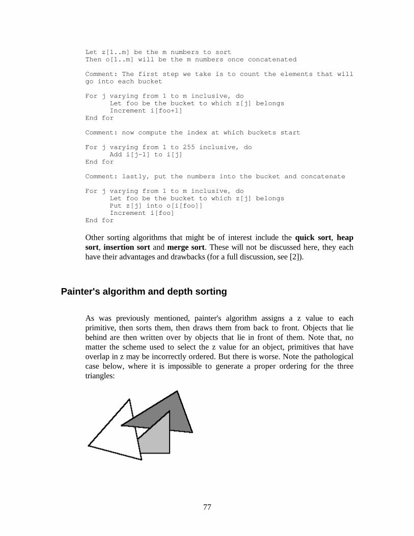
77

Let z[1..m] be the m numbers to sortThen o[1..m] will be the m numbers once concatenated

Comment: The first step we take is to count the elements that willgo into each bucket

For j varying from 1 to m inclusive, doLet foo be the bucket to which z[j] belongsIncrement i[foo+1]

End for

Comment: now compute the index at which buckets start

For j varying from 1 to 255 inclusive, doAdd i[j-1] to i[j]

End for

Comment: lastly, put the numbers into the bucket and concatenate

For j varying from 1 to m inclusive, doLet foo be the bucket to which z[j] belongsPut z[j] into o[i[foo]]Increment i[foo]

End for

Other sorting algorithms that might be of interest include the quick sort, heapsort, insertion sort and merge sort. These will not be discussed here, they eachhave their advantages and drawbacks (for a full discussion, see [2]).

Painter's algorithm and depth sorting

As was previously mentioned, painter's algorithm assigns a z value to eachprimitive, then sorts them, then draws them from back to front. Objects that liebehind are then written over by objects that lie in front of them. Note that, nomatter the scheme used to select the z value for an object, primitives that haveoverlap in z may be incorrectly ordered. But there is worse. Note the pathologicalcase below, where it is impossible to generate a proper ordering for the threetriangles:

78

In this case, it is necessary to cut one triangle into two parts and sort the partsindividually.

A way of handling all cases is as follows. Assign a z value to all polygons equal tothe vertex belonging to the polygon that has the largest z coordinate value in eyespace. Then sort as per painter's algorithm. Before actually drawing, we need to doa postsort stage to make sure the ordering is correct for polygons that have zoverlap.

Assuming we sorted in increasing values of z, it means that we need only tocompare the last polygon with the consecutive previous polygons for which thefurthest point is in the last polygon's z span. Once the last polygon is processed,we will not touch it anymore (unless the last polygon is moved to some otherposition in the list). Thus, we just consider the list to be one element shorter andrecurse the algorithm.

The steps that should be taken are as follow (P and Q are the polygons we arecomparing).

1- Check whether the polygons x and y extent overlap on screen. If they do not,there is no need to compare the polygons. Otherwise, we are undecided (go to 2)

2- Check on what side of P's plane the eye lies. If Q lies entirely on that side of P'splane, Q is considered to be in front of P. If Q lies entirely on the opposite side ofthe eye in relation to P's plane, then P is in front of Q. If Q crosses P's plane, weare still undecided.

3- Repeat 2 above, but with Q and P inverted.

4- Check if the polygons overlap on screen (find whether the edges of thepolygons intersect)

Once a polygon has been moved in the list, mark it so that it is not moved again. Ifone of the above steps would say that a polygon that has already been moved inthe list should be moved again, then you will have to use the last resort, clipping.Cutting up the triangle into pieces (clipping) will be described later.

Of course, one needs not to perform all these tests if they are deemed to be moreexpensive than clipping. For instance, the only tests one could do is test foroverlap in z, then x and y on screen, then check for step 2 and if it is stillunresolved, simply clip the polygons and put the pieces where they belong.

When polygon ordering can not be resolved, pick one of the two polygons forclipping plane and clip the other polygon with it. Then, insert the two pieces at theappropriate positions in the list.

79

A very nice way of doing all these tests is as follows. Calculate bounding boxes forz value in 3d, and u,v in 2d (screen space, after perspective transform) of thepolygon. Then, sort the bounding boxes in x, u and v. This can be done in lineartime using the radix sort algorithm (or by exploiting coherence in a comparisonsort algorithm). Then, only the polygons for which the bounding boxes overlap inall three axis need to be checked further.

Z-Buffering

This algorithm tends to be slightly slower than painter's algorithm for low numberof polygons (less than 5000). It would appear that it would gain as the number ofpolygons increases though.

The idea is to make an array of z or 1/z values, one for each pixel. As you draw apolygon, compute the z or 1/z value at a pixel, compare it with the current valuefor the pixel, and if closer, draw, otherwise, do not draw.

This algorithm has the advantage that it requires no sorting whatsoever. However,the algorithm performs one comparison per pixel, which tends to be a bitexpensive. Also, memory requirements tend to be bigger than other algorithms.Nevertheless, the simplicity of the implementation makes it very attractive.

As a side note on evaluating z or 1/z, the latter can be shown to be linear while theformer is not (we did this in the perspective chapter). Thus, it will likely bepreferable to store 1/z values instead of z, because they can typically be computedmuch more quickly. The mathematics of that are shown below.

Let Ax+By+Cz=D be the plane equation for the polygon in eye space. Let (u,v)denote the pixel on screen, and let the perspective projection equation be u=px/zand v=qy/z for some constants p and q. This can be rewritten as:

x=uz/p y=vz/q

Auz/p+Bvz/q+Cz=D

z(Au/p+Bv/q+C)=D

And then, depending whether we are interested in z or 1/z, we get:

z=D/(Au/p+Bv/q+C)

or

1/z=A/(Dp)u+B/(Dq)v+C/D

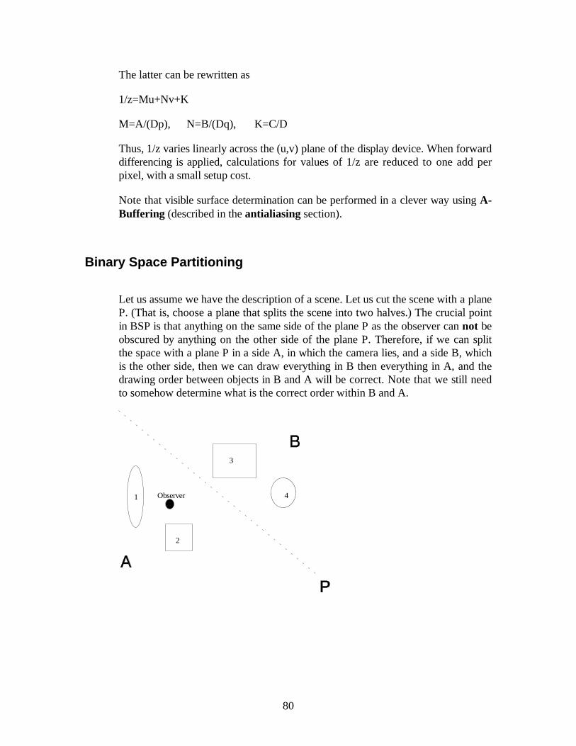
80

The latter can be rewritten as

1/z=Mu+Nv+K

M=A/(Dp), N=B/(Dq), K=C/D

Thus, 1/z varies linearly across the (u,v) plane of the display device. When forwarddifferencing is applied, calculations for values of 1/z are reduced to one add perpixel, with a small setup cost.

Note that visible surface determination can be performed in a clever way using A-Buffering (described in the antialiasing section).

Binary Space Partitioning

Let us assume we have the description of a scene. Let us cut the scene with a planeP. (That is, choose a plane that splits the scene into two halves.) The crucial pointin BSP is that anything on the same side of the plane P as the observer can not beobscured by anything on the other side of the plane P. Therefore, if we can splitthe space with a plane P in a side A, in which the camera lies, and a side B, whichis the other side, then we can draw everything in B then everything in A, and thedrawing order between objects in B and A will be correct. Note that we still needto somehow determine what is the correct order within B and A.

Observer1

2

3

4

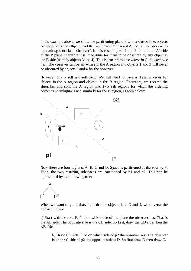
81

In the example above, we show the partitioning plane P with a dotted line, objectsare rectangles and ellipses, and the two areas are marked A and B. The observer isthe dark spot marked "observer". In this case, objects 1 and 2 are on the "A" sideof the P plane, therefore it is impossible for them to be obscured by any object inthe B side (namely objects 3 and 4). This is true no matter where in A the observerlies. The observer can be anywhere in the A region and objects 1 and 2 will neverbe obscured by objects 3 and 4 for the observer.

However this is still not sufficient. We still need to have a drawing order forobjects in the A region and objects in the B region. Therefore, we recurse thealgorithm and split the A region into two sub regions for which the orderingbecomes unambiguous and similarly for the B region, as seen below:

Observer1

2

3

4

Now there are four regions, A, B, C and D. Space is partitioned at the root by P.Then, the two resulting subspaces are partitioned by p1 and p2. This can berepresented by the following tree:

When we want to get a drawing order for objects 1, 2, 3 and 4, we traverse thetree as follows:

a) Start with the root P, find on which side of the plane the observer lies. That isthe AB side. The opposite side is the CD side. So first, draw the CD side, then theAB side.

b) Draw CD side. Find on which side of p2 the observer lies. The observeris on the C side of p2, the opposite side is D. So first draw D then draw C.

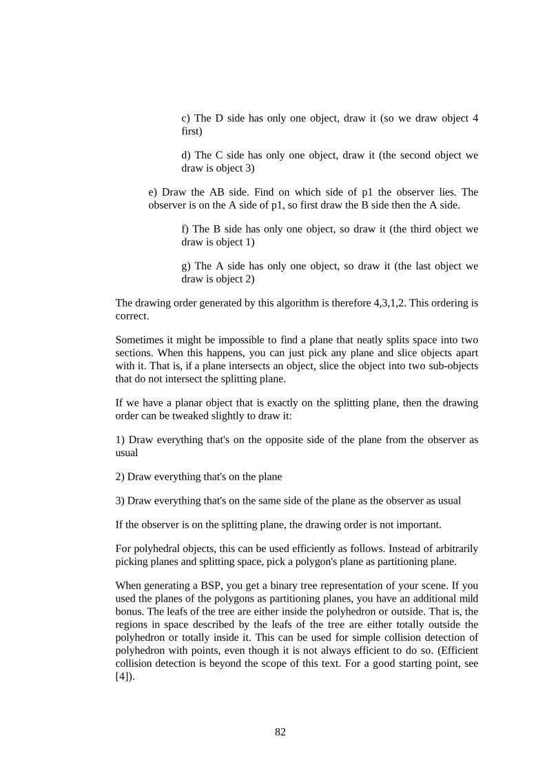
82

c) The D side has only one object, draw it (so we draw object 4first)

d) The C side has only one object, draw it (the second object wedraw is object 3)

e) Draw the AB side. Find on which side of p1 the observer lies. Theobserver is on the A side of p1, so first draw the B side then the A side.

f) The B side has only one object, so draw it (the third object wedraw is object 1)

g) The A side has only one object, so draw it (the last object wedraw is object 2)

The drawing order generated by this algorithm is therefore 4,3,1,2. This ordering iscorrect.

Sometimes it might be impossible to find a plane that neatly splits space into twosections. When this happens, you can just pick any plane and slice objects apartwith it. That is, if a plane intersects an object, slice the object into two sub-objectsthat do not intersect the splitting plane.

If we have a planar object that is exactly on the splitting plane, then the drawingorder can be tweaked slightly to draw it:

1) Draw everything that's on the opposite side of the plane from the observer asusual

2) Draw everything that's on the plane

3) Draw everything that's on the same side of the plane as the observer as usual

If the observer is on the splitting plane, the drawing order is not important.

For polyhedral objects, this can be used efficiently as follows. Instead of arbitrarilypicking planes and splitting space, pick a polygon's plane as partitioning plane.

When generating a BSP, you get a binary tree representation of your scene. If youused the planes of the polygons as partitioning planes, you have an additional mildbonus. The leafs of the tree are either inside the polyhedron or outside. That is, theregions in space described by the leafs of the tree are either totally outside thepolyhedron or totally inside it. This can be used for simple collision detection ofpolyhedron with points, even though it is not always efficient to do so. (Efficientcollision detection is beyond the scope of this text. For a good starting point, see[4]).

83

All this brings up the subject of generating an optimal BSP tree. There are manyproblems with that. The first is the definition of optimal. In the collision detectioncase (which is not too efficient anyway, but deserves mention), optimal oftenmeans shallowest tree. For visible surface determination, minimizing the number oftriangle clipping is important, as well as minimizing the number of nodes (which isa consequence of clipping). In both cases, the problem turns out to be extremelyhard (NP-Hard). In the "minimizing the tree depth" field, a greedy algorithm thatpicks the plane that splits space as evenly as possible might do well. However,when trying to minimize the number of polygon clips, it's harder to get goodheuristics.

Merging BSP trees is also a very tough problem. Basically it's at least as hard asgenerating a new BSP tree from scratch. However, it is possible to cut corners.

If we have a very large maze-like scene (for example), and a small objectnavigating through it, we can do as follows. We treat the small object as a point,just like the observer, and traverse the BSP tree of the maze scene to find wherethe "punctual" object belongs in the BSP tree. Once we have found it, we insertthe "punctual" object's BSP tree at that point in the maze BSP tree. This will workrelatively well so long as the small object dos not come close enough to corners inwalls to cause ambiguities in the display ordering.

It is also possible to insert several objects this way in the maze BSP.

This algorithm can be very efficient if we have many objects spread over a largearea where inter object ordering can be determined easily, but the objectsthemselves are complex so intra object visual surface determination is nontrivial.

Note that a BSP can be processed through an affine transform and still remainvalid if proper care is taken. This means that we can move a binary spacepartitioned object around, or we can move the observer in the BSP object (thesetwo are equivalent anyway) without fear of the algorithm crumbling. Therefore, itis possible to have a few flying BSP objects at the same time, for instance.

84

Lighting models

Introduction

After all we have covered, we still have to decide how much light gets reflected offthings and such, and how it gets reflected. For example, some objects that arefacing towards a light source will appear much more bright, perhaps with a verybrilliant spot somewhere, than objects facing away from it. Objects also castshadows, which are much harder to compute. We might also want to somehowtake into account that a certain quantity of light bounces off everything and lightsup things equally from all directions.

Furthermore, we might want to vary the intensity of light across a given polygon,especially if these polygons are big. If not, one gets a somewhat ugly effect calledmach banding where the contrast between faces gets amplified by our brain andeyes. This will raise the question of how the light should vary across a polygon,and why.

The first part discusses actual lighting models, and the second discusses shadingalgorithms for rasterization of nonuniformly shaded polygons.

Lighting models

The most basic idea we can have is to make light intensity a function of the anglebetween the direction of the light rays from the light source to a point, and thenormal to the point. This is called diffuse lighting. This means that light reflects offthe face equally in all directions, so the direction in which the eye is not relevant.

Looking back on the vector algebra chapter, we had a definition of angle with thedot product. This is written as:

Cosθ=A•B/(|A|×|B|)

85

If A is the plane normal (of unit length), then |A| is 1 and can be removed from theequation. B would be the vector from light source to point to be lit. Then, wemake light intensity a function of Cosθ, which is calculated to be A•B/|B|, which isfairly easy to calculate. Note that if θ is less than π/2, it means that the face isactually facing away from the light source, in which case it should not receive anylight from that light source. This can be recognized when A•B/|B|>0.

Usually, one makes the intensity of the light received from a light source A•B/|B|times some negative constant (since positive values of A•B/|B| mean that the faceis facing away and that intensity is then 0).

One might want to take into account the fact that light usually diminishes thefurther away you are from a light source. Physics say that light intensity isinversely proportional to the square of the distance to the light source. This can bewritten as k/|B|2, and multiplying that by the value previously given:

I=k×A•B/|B|3

However, as experimentation shows, it is sometimes useful to use some otherfalloff than square of distance. Generally, people have been using a second degreepolynomial of |B|. However, if we try the specific case of linear falloff, we get thisvery interesting simplification:

I=k×A•B/|B|2

If B=(a,b,c), then |B|=(a2+b2+c2)1/2. Thus, |B|2=a2+b2+c2, which eliminates thesquare root, which is usually the most expensive calculation we have.

The question of what point on the polygon should be used for calculating thevector B from light source to the point on the polygon is answered as follows.Theoretically, B should be recalculated for each point on the polygon. This mightturn out to be expensive, and a constant B is then used across the polygon. In thiscase, however, the B/|B|2 factor should be calculated only once for the wholepolygon.

The Phong illumination model also includes a specular component. In that case,a function of the angle between the ideal reflection vector and the eye-to-pointvector is added. The reflection vector R is the direction in which the light shouldbe most reflected by the surface. R can be shown to be

R=2A(A•B)-B

(remember that A is the plane normal and B the light vector and note that A and Bshould be normalized).

86

Let V be the vector from the observed point to the eye, normalized. Then, afunction of R•V can be added to the calculated intensity (before fallout due todistance is taken into account), which will add a specular like highlight to theshading. Mr. Phong Bui-Tuong used the following specular component:

k×(R•V)α

where α is the so-called specular reflection exponent and k is the specularreflection coefficient. The larger the α, the more punctual the reflection. Thelarger the k, the more intense the reflection. Values of α around 1-5 yield almostno specular reflection, while a value of 300 or more yields a sharp spot. Note thatif a too large k is chosen, the image will look washed out or overexposed.

These calculations are done on a per light source basis, and should be summed.Ambient light can also be added.

Shadow casting involves more complex computations which will not be discussedhere.

Smooth shading

The simplest form of polygon shading calculates one value of intensity and usesthat value across the whole polygon.

The other forms of shading require that we first examine our polyhedral model ofobjects. The assumption we are making is that the polyhedral model is really anapproximation to a curved object. Thus, we would like the normal vectors and theshading intensity to vary smoothly across the surface of the objects, just as it doeson a curved surface.

The usual way of accomplishing this is by computing a pseudo normal vector ateach vertex. (Keep in mind that a point in 3d has no normal vector, ergo we call itpseudo-normal.) That pseudo-normal per vertex is not the normal of the vertex,but rather the normal we think represents best the curved surface at that point. Ifwe have actual information about the curved surface, we should use thatinformation if we can to compute the pseudo-normal. Otherwise, one good way ofdoing this is by computing the weighted sum of the faces that touch the vertex. Forexample, you could sum all normals of the faces that touch the vertex and thennormalize. Or, you could make each face's contribution to the pseudo-normal afunction of the face's area or the angle made by that face at the vertex, and so on.For ease in calculations, pseudo-normals should be made unit in length.

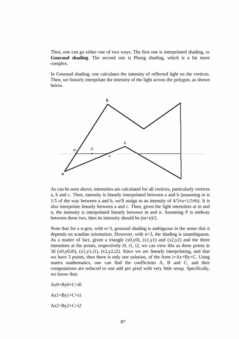
87

Then, one can go either one of two ways. The first one is interpolated shading, orGouraud shading. The second one is Phong shading, which is a bit morecomplex.

In Gouraud shading, one calculates the intensity of reflected light on the vertices.Then, we linearly interpolate the intensity of the light across the polygon, as shownbelow.

As can be seen above, intensities are calculated for all vertices, particularly verticesa, b and c. Then, intensity is linearly interpolated between a and b (assuming m is1/5 of the way between a and b, we'll assign m an intensity of 4/5×a+1/5×b). It isalso interpolate linearly between a and c. Then, given the light intensities at m andn, the intensity is interpolated linearly between m and n. Assuming P is midwaybetween these two, then its intensity should be (m+n)/2.

Note that for a n-gon, with n>3, gouraud shading is ambiguous in the sense that itdepends on scanline orientation. However, with n=3, the shading is unambiguous.As a matter of fact, given a triangle (x0,y0), (x1,y1) and (x2,y2) and the threeintensities at the points, respectively i0, i1, i2, we can view this as three points in3d (x0,y0,i0), (x1,y1,i1), (x2,y2,i2). Since we are linearly interpolating, and thatwe have 3 points, then there is only one solution, of the form i=Ax+By+C. Usingmatrix mathematics, one can find the coefficients A, B and C, and thencomputations are reduced to one add per pixel with very little setup. Specifically,we know that:

Ax0+By0+C=i0

Ax1+By1+C=i1

Ax2+By2+C=i2

88

Which can be represented in matrix form as:

.

x0

x1

x2

y0

y1

y2

1

1

1

A

B

C

i0

i1

i2

or,

XK=G, where

X

x0

x1

x2

y0

y1

y2

1

1

1

K

A

B

C

G

i0

i1

i2

Therefore, we have that K=X-1G, which solves for K.

As a special note, it should be remembered that a similar process can be used forany type of linear interpolation across the surface of a polygon.

It is easy to demonstrate that no point within the polygon will be brighter or darkerthan the brightest or darkest vertex, respectively. If a specular highlight should fallwithin a polygon, Gouraud shading will miss it entirely.

Phong shading (not to be confused with the Phong illumination model) worksaround this the following way. Instead of interpolating the intensity linearly, itinterpolates the (x,y,z) values of the pseudo-normals linearly, then normalizes, andthe does the lighting calculations once per pixel. As a side note, the interpolationof x, y and z can be done as we just saw for Gouraud shading.

As you might imagine, this is extremely expensive. Many approximations,workarounds and somesuch have been devised. Here we will study one suchapproximation.

We will interpolate the (x,y) value of pseudo-normals linearly, but we will setz=(1-x2-y2)1/2. Note that we still have a square root. However, since z is afunction of x and y only, and that x and y vary between -1 and +1 only, we canmake a lookup table for z, which makes it a lot faster. Then we can do the lightingcalculations. However, this is still a bit slow. If we know our light vector to beconstant across the screen, then we can optimize it further.

89

Assuming the light vector is (0,0,1), then the lighting calculations for diffuseshading only is (x,y,z)• (0,0,1). This simplifies to z, which is (1-x2-y2)1/2, which isthe value we stored in the lookup table. So, interpolate (x,y) linearly and lookupintensity in the lookup table. As a matter of fact, one can even put some othervalues than (1-x2-y2)1/2 in the lookup table. These can be used to achievespecular highlights, multiple light sources, or some nice metal/chrome/mirroreffects.

A note on the "mirror" effect. If we imagine that we have a sphere centered on ourobject with an extremely large radius, and the in side of the sphere is paved with atexture (example: stars & stellar objects) and the object has a mirror surface, thenthe environment (textured sphere) should be reflected on it. The perspectivecalculations and other things make this complex. However, we can simplify thingsthis way. We assume that the vector from eye to object (eye vector) is constantover all of the surfaces of the object (which is normally true only in parallelprojections, but will be almost true if the object has little perspective distortion).Second, we assume that the sphere has a large radius enough that the point of thesphere which is reflected by a point of the object only depends on the eye vectorand the surface normal.

In this case, we can interpolate the surface normal Phong-style, then use that tocompute the reflected point from the sphere using the eye vector. However, thecomputations are still quite expensive. We can simplify them by using the hackwhere we interpolate x and y linearly and then set z=(1-x2-y2)1/2. Then, thenormal vector of a point on the surface is entirely determined by x and y. In thiscase, the reflected point on the sphere depends on x, y and the eye vector. Whatwe can do is assume a fixed eye vector, then make a lookup table (which is thenonly dependant on x and y, which is manageable) to find what point on the sphereit reflects to.

Hence this simplifies to interpolating the (x,y) component of a surface normalacross the screen, then looking it up in a lookup table that contains the color of thecorresponding reflected point on the sphere.

Texture mapping & variants on the same theme

Texture mapping is the process by which we give a polygon its own planarcoordinate system, with two base vector that lie in the polygon's plane, and avector for the position of a point in the plane. Specifically, if u and v lie in theplane of the polygon, and w is a point in the plane of the polygon (for example, avertex), then the plane equation for the polygon can be written as:

au+bv+w

90

where (a,b) are the texture coordinates on the polygon. Once we have (a,b), wecan assign different properties to different (a,b) pairs. For example, we can makethe color of the polygon a function of (a,b), which corresponds to classical texturemapping. Another thing we can do is perturb the surface normal of the polygonwith some function of (a,b), which corresponds to bump mapping.

As it is, the Phong shading approximation we saw in the last bit of the precedingsection is essentially a texture mapping trick.

Note that it is possible to have several different coordinate systems for the samepolygon, if several different textures have to be applied (ie, one for the actualtexture mapping, another one for the phong shading, another one for bumpmapping, and who knows what else).

What we have said in this section up to now is (relatively) independent of theprojection used. Now we will consider the type of projection used.

In a parallel projection, linear interpolation, just like we did for Gouraud, acrossthe projected surface is correct (so long as the surface is planar). However, whenperspective projecting, linear interpolation is generally wrong. For an elaboratediscussion of the texture mapping equation in the perspective projection case, seethe perspective chapter.

If the plane of the perspectively projected polygon is perpendicular to the z axis,then linear interpolation is exact. As the angle between the plane of the polygonand the z axis moves away from 90 degrees, linear interpolation becomes more andmore wrong. If the polygons are small enough on screen, the perspective distortionmight now show, but for larger and more angled polygons, it is quite apparent.

Linear interpolation may suffice for some purposes on low end platforms andgames, but a correction for perspective will definitely be needed for more seriousapplications, as discussed in the perspective chapter.

91

Computer graphics related problems

Introduction

In the process of learning computer graphics, one comes across several of theclassical questions in one version or another. These include "how do I compute theplane normal of a triangle" or more generally "how do I compute the plane normalof a polygon, preferably using all vertices to minimize error", "how do I make anormal that points outwards" and such.

These technical questions need to be addressed individually, since they typicallyhave very little in common. First will be covered generating normals that pointoutwards for polygons. An application of that will be covered, which istriangulation of a concave polygon. Computation of a normal for any polygon isthen considered, by using all vertices to compute it. Then will be covered theproblem of generating plane normals that point outwards of a polyhedron, whichrelies on edge normals that point outwards of a polygon.

Generating edge normals

It will prove to be essential for the later problems to have normals for the edgesthat point outwards from the polygon. We might as well start by saying that for anedge of slope m, the normal would be (-m,1) unitized. The second preliminary isdefining modulo space addition and subtraction.

Let a and b be integers of modulo n space. Then, a⊕ b is defined to be (a+b)%n,where x%y means "remainder of the division of x by y" (the remainder is alwayspositive, between 0 and y-1). Similarly, aΘb is defined to be (a-b)%n. As anexample, let's assume we are working in modulo 8 space. Then,

3⊕ 2=5%8=5 5⊕ 6=11%8=3 4Θ3=1%8=1 4Θ7=-3%8=5

The first step is to generate normals for all edges by calculating (-m,1) andunitizing it. These normals will not all be oriented correctly.

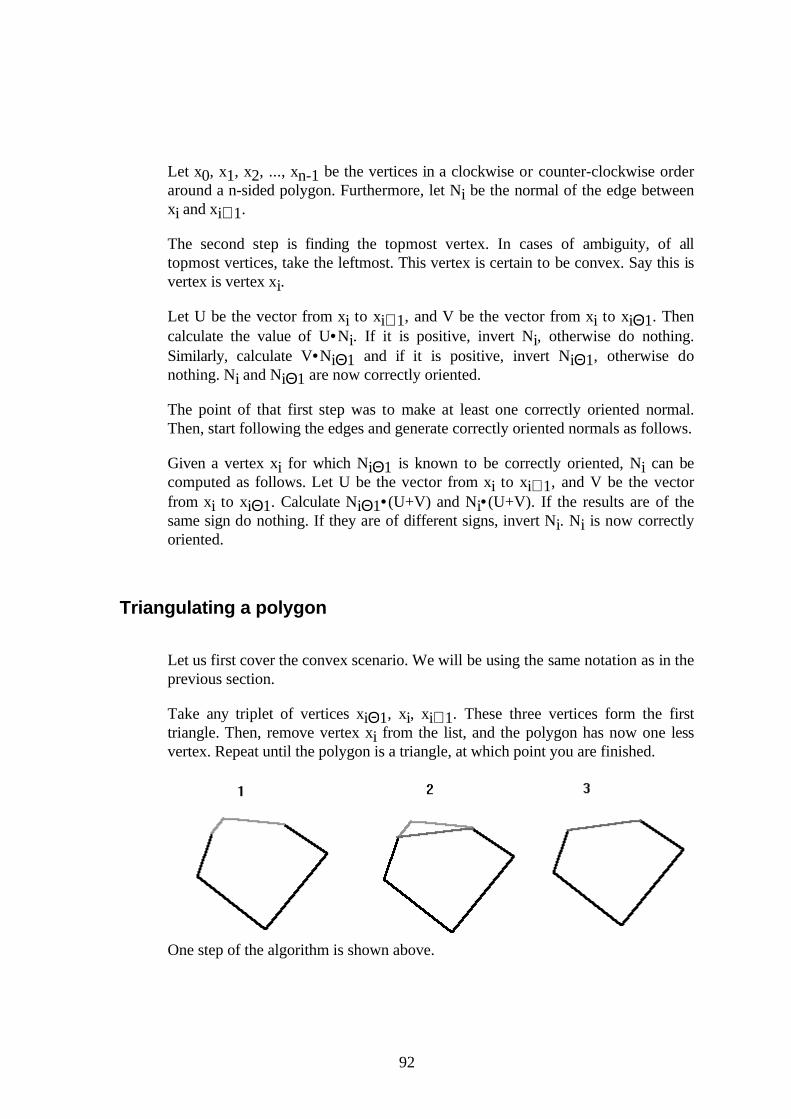
92

Let x0, x1, x2, ..., xn-1 be the vertices in a clockwise or counter-clockwise orderaround a n-sided polygon. Furthermore, let Ni be the normal of the edge betweenxi and xi⊕ 1.

The second step is finding the topmost vertex. In cases of ambiguity, of alltopmost vertices, take the leftmost. This vertex is certain to be convex. Say this isvertex is vertex xi.

Let U be the vector from xi to xi⊕ 1, and V be the vector from xi to xiΘ1. Thencalculate the value of U•Ni. If it is positive, invert Ni, otherwise do nothing.Similarly, calculate V•NiΘ1 and if it is positive, invert NiΘ1, otherwise donothing. Ni and NiΘ1 are now correctly oriented.

The point of that first step was to make at least one correctly oriented normal.Then, start following the edges and generate correctly oriented normals as follows.

Given a vertex xi for which NiΘ1 is known to be correctly oriented, Ni can becomputed as follows. Let U be the vector from xi to xi⊕ 1, and V be the vectorfrom xi to xiΘ1. Calculate NiΘ1• (U+V) and Ni• (U+V). If the results are of thesame sign do nothing. If they are of different signs, invert Ni. Ni is now correctlyoriented.

Triangulating a polygon

Let us first cover the convex scenario. We will be using the same notation as in theprevious section.

Take any triplet of vertices xiΘ1, xi, xi⊕ 1. These three vertices form the firsttriangle. Then, remove vertex xi from the list, and the polygon has now one lessvertex. Repeat until the polygon is a triangle, at which point you are finished.

One step of the algorithm is shown above.

93

The concave scenario is a bit more complicated. What we will do is split theconcave polygon into smaller polygons, eventually resulting in either triangles orconvex polygons that can be triangulated as above.

Find a vertex that is concave. Let U be the vector from xiΘ1 to xi. Then, vertex xiis concave if and only if U•Ni is more than zero. Loop through the vertices untilyou find such a vertex. If you do not find one, then the polygon is convex andtriangulate it as above.

From that vertex, find a second vertex xj for which the line segment from xi to xjdoes not intersect any other edge. Then, insert that new edge, making twopolygons, one that has the vertices xi, xi⊕ 1, xi⊕ 2, ..., xj, and one that has verticesxj, xj⊕ 1, xj⊕ 2, ..., xi. Re-apply the algorithm on these two smaller polygons.

It can be demonstrated that using the above algorithm on a n sided polygon willgenerate exactly n-2 triangles.

Computing a plane normal from vertices

It can be shown that the (P,Q,R) components of the normal vectors areproportional to the signed area of the projection of the polygon on the yz, xz andxy plane respectively.

The signed area of a polygon in (u,v) coordinates can be shown to be:

A(u,v)=1/2×∑0≤i<n(vi+vi⊕ 1)×(ui⊕ 1-ui)

where (ui, vi) are the coordinates of vertex xi in 2d.

Since we're not really interested in the signed area, but some constant time thesigned area, the 1/2 can be safely ignored without loss of precision.

Given a polygon in 3d, one can compute the above with:

P=A(y,z) Q=A(z,x) R=A(x,y)

Or, if you want, P is the area as calculated using only the y and z components ofthe points in 3d, Q is the area as calculated using the z and x components of pointsin 3d, and R is the area as calculated using the x and y components of points in 3d.

Once this value of (P,Q,R) is known, the result should be normalized, and thencorrect orientation should be checked as described hereafter.

It should be noted that the A(u,v) equation simplifies to

94

A(u,v)=1/2×[(u0-u1)(v0-v2)-(v0-v1)(u0-u2)]

in the case of a triangle. Again, the 1/2 constant can be ignored for normalgeneration purposes.

Generating correctly oriented normals for polyhedra

In some cases, normal orientation is implicit in the object description we have. Forinstance, some modelers output all vertices in a counterclockwise manner whenseen from above. If this is the case, then all that is needed is that the normal becomputed in a specific way, without changing the ordering of the vertices. Thenthe normals will be correctly oriented.

If this is not the case, we need some form of algorithm to ensure proper normalorientation.

For this task, we need to have computed the normals to the edges to for allpolygons making up the polyhedron, each in their respective plane of course. Theedges normals in the polygons planes can be localized in space for the polyhedron,we are going to use this. Note that each edge is connected to two polygons, thushas two normals, one per polygon.

Find the vertex with the smallest x coordinate. In case of ambiguity, resolve withthe smallest y coordinate. In case of ambiguity, resolve with the smallest z value.This vertex is known to be convex. Take all edges connected to that vertex, andfind the vector U that is the sum of all edge normals (two per edge). Then, foreach face touching the point, calculate A•U, where A is the face normal. If theresult is negative, invert A, otherwise leave it as it is. All such faces now havecorrectly oriented normal.

From this point, traverse all faces, propagating correctly oriented normals asfollows. Let us assume we have two faces F1 and F2, and that F1's normal iscorrectly oriented. Let A1 and A2 denote F1 and F2's normals respectively. Pickan edge shared by F1 and F2, and compute U, the sum of the two edge normals.Then evaluate A1•U and A2•U. If they are of different signs, invert A2, otherwiseleave it that way. A2 is now correctly oriented.

A special note, if the dot products are very close to zero, the face should beinitialized with the same normal, and marked as ambiguous. Later, if you can findanother face to help you better determine the orientation of that face, use thatnormal instead. At any rate, ambiguous faces should be avoided when propagatingnormal orientation.

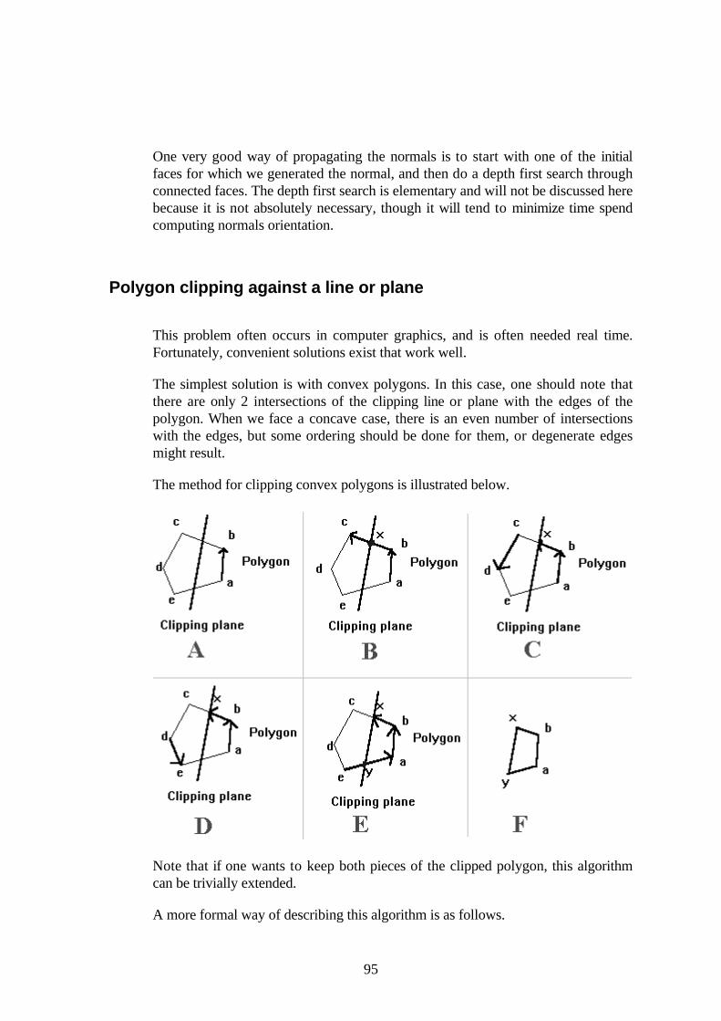
95

One very good way of propagating the normals is to start with one of the initialfaces for which we generated the normal, and then do a depth first search throughconnected faces. The depth first search is elementary and will not be discussed herebecause it is not absolutely necessary, though it will tend to minimize time spendcomputing normals orientation.

Polygon clipping against a line or plane

This problem often occurs in computer graphics, and is often needed real time.Fortunately, convenient solutions exist that work well.

The simplest solution is with convex polygons. In this case, one should note thatthere are only 2 intersections of the clipping line or plane with the edges of thepolygon. When we face a concave case, there is an even number of intersectionswith the edges, but some ordering should be done for them, or degenerate edgesmight result.

The method for clipping convex polygons is illustrated below.

Note that if one wants to keep both pieces of the clipped polygon, this algorithmcan be trivially extended.

A more formal way of describing this algorithm is as follows.

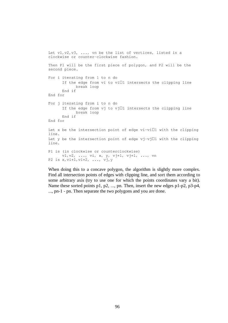
96

Let v1,v2,v3, ..., vn be the list of vertices, listed in aclockwise or counter-clockwise fashion.

Then P1 will be the first piece of polygon, and P2 will be thesecond piece.

For i iterating from 1 to n doIf the edge from vi to vi ⊕ 1 intersects the clipping line

break loopEnd if

End for

For j iterating from i to n doIf the edge from vj to vj ⊕ 1 intersects the clipping line

break loopEnd if

End for

Let x be the intersection point of edge vi-vi ⊕ 1 with the clippingline.Let y be the intersection point of edge vj-vj ⊕ 1 with the clippingline.

P1 is (in clockwise or counterclockwise)v1,v2, ..., vi, x, y, vj+1, vj+1, ..., vn

P2 is x,vi+1,vi+2, ..., vj,y

When doing this to a concave polygon, the algorithm is slightly more complex.Find all intersection points of edges with clipping line, and sort them according tosome arbitrary axis (try to use one for which the points coordinates vary a bit).Name these sorted points p1, p2, ..., pn. Then, insert the new edges p1-p2, p3-p4,..., pn-1 - pn. Then separate the two polygons and you are done.

97

Quaternions

Introduction

In this chapter, a good understanding of basic mathematics is assumed. I also havebeen extremely lazy and I’m not giving any justifications whatsoever. Someday,hopefully, this will be righted. It is possible to do very much everything that isdescribed here using only matrices with a good knowledge of linear algebra. Forinstance, as a first step, we can find a matrix that rotates about an arbitrary unitvector by a specific angle. Then, if we want to interpolate linearly between twoorientations, we can proceed as follows. First find the matrix M that expresses thetransform from the first orientation to the second orientation. Then find theeigenvector of that matrix, this is the desired axis of rotation. Then linearlyinterpolate the angle from 0 to whatever angle the two orientations make.

Let us recall complex numbers, which have the form a+bi, where i2=-1. Thesecomplex numbers can also be represented in polar or exponential form . I willinterest myself mainly with the latter. The exponential form of a complex number isZ=r×exp(iθ), where (r,θ) are the polar coordinates of Z in the complex plane. Allpoints in the plane can be represented by a complex number. Let B be a unitquaternion (that is, of the form B=exp(iθ0)). Recall that, when multiplying twocomplex numbers, we multiply the modules and add the angles. Let us multiply Zby B. Then, we get ZB=r×exp(iθ+θ0), or Z rotated by θ0.

The morale of this story is that unit complex numbers can be used to representrotations in the plane.

We will now develop a similar tool for modeling rotations in 3d. A quaternion Qwill be of the form Q=W+Xi+Yj+Zk, where 1, i, j and k are linearly independentquantities (and i, j and k are linearly independent imaginary numbers). Then, wewill define quaternion multiplication, by using the following basic rules:

i2=j2=k2=-1, ij=-ji=k, jk=-kj=i, ki=-ik=j.

It will so turn out that, similarly to unit complex numbers represent rotations in theplane, unit quaternions will represent rotations in 3d.

98

Obviously, this is a lot of work for "just another representation of rotations in 3d",especially where matrices work fine. Indeed, even if one is using quaternions torepresent orientations, one will typically convert to a matrix when actualtransformations are required. The main advantage of quaternions is forinterpolating between two orientations in a useful manner, and mayhaps also for acompact representation of orientations.

Preliminaries

Several notations can be used to write quaternions. The following are allequivalent:

Q=W+Xi+Yj+Zk

Q=<W, A> with A=(X,Y,Z) (a real number W, with a 3d vector (X,Y,Z))

Q=(W,X,Y,Z) (a 4d vector)

We can define a multiplication operation that respects the following:

i2=j2=k2=-1, ij=-ji=k, jk=-kj=i, ki=-ik=j.

<a1, v1>×<a2,v2>=<a1a2-v1•v2 , s2v1+s1v2+v1×v2>

Of course, a1 and a2 are real numbers and v1 and v2 are 3d vectors.

The norm or module of a quaternion Q=(W,X,Y,Z) is defined as the euclidiannorm of vector (W,X,Y,Z). A unit quaternion is a quaternion for which its normis 1.

The conjugate of quaternion Q=<W,A> is defined as Qc=<W,-A>.

If we have the quaternion

Q=(0,v)=(0,X,Y,Z)

and the unit quaternion

U=(cos(θ/2),sin(θ/2)×V)

where V is a unit vector, and

Q'=(0,v')=U×Q×Uc

then it can be shown that v' is v rotated about V by an angle of θ.

99

Note that this implies that the two unit quaternions Q and -Q represent the samerotation.

Conversion between quaternions and matrices

The quaternion Q=(W,X,Y,Z) (assuming Q is unit) is equivalent, when interpretedas a rotation, to the matrix:

1 .2 Y2 .2 Z

2

..2 X Y ..2 W Z

..2 X Z ..2 W Y

..2 X Y ..2 W Z

1 .2 X2 .2 Z

2

..2 Y Z ..2 W X

..2 X Z ..2 W Y

..2 Y Z ..2 W X

1 .2 X2 .2 Y

2

By examining the above matrix, it is easy to find, given an orthonormal orientationmatrix, the corresponding quaternion. First, compute W.

m11+m22+m33=3-4X2-4Y2-4Z2

(m11+m22+m33+1)/4=1-X2-Y2-Z2

But |(W,X,Y,Z)|=1 hence W2+X2+Y2+Z2=1 hence

W=[(m11+m22+m33+1)/4]1/2

Then, compute X, Y and Z.

X=(m32-m23)/4W

Y=(m13-m31)/4W

Z=(m21-m12)/4W

Orientation interpolation

Often, we might only have an initial orientation, and a desired orientation at somepoint in the future, and no data in between. In this case, it might be desirable tointerpolate the orientations between these two key orientations. Assuming no otherdata is available, quaternion interpolation is very appropriate.

100

This could be done with Euler angles. However, several problems arise when wedo so. We can very difficultly control the exact path of the rotation, or the speedfor that matter. We also get a problem called "Gimbal lock", where the objectappears to stop turning for a brief moment, and then starts again in an odddirection.

Using quaternions, we get none of these problems. Speed of rotation can be madeconstant, and the path of the rotation will be that of the shortest arc. However, weget numerical problems when the rotation is close to 180 degrees. Also, we willneed to interpolate through more than 2 quaternions if we want to rotate by morethan 180 degrees.

The idea is to picture the unit quaternions as being on the unit hypersphere in 4d.Then, we can find the shortest arc over that hypersphere between these twoquaternions, and interpolate linearly the angle along that arc.

Given two unit quaternions, q1 and q2, let us first find the angle between them. Bydefinition of angle as a function of dot product, we have:

φ=acos(q1•q2)

Then, let us have a parameter t that varies from 0 to 1. Then, the quaternion givenby:

q( )t .sin( ).( )1 t φ

sin( )φq1 .sin( ).t φ

sin( )φq2

will give uniformly distributed orientations between q1 and q2 as t varies from 0 to1. In particular, q(0)=q1, q(1)=q2. This is called spherical linear interpolation ,or SLERP.

Note that we didn't check if we were using the shortest arc or the longest on thegreat circle. In order to take the shortest path, we simply check that

(q1-q2)• (q1-q2)>(q1+q2)• (q1+q2)

If that is false, replace q2 by -q2 (this is allowed since Q and -Q represent the samerotation).

The above formula will have numerical difficulties when φ is close to 0 or π. When φ is close to 0, we can replace the SLERP with a simple linear interpolation. E.g.q(t)=(1-t)q1+tq2. When φ is close to π, we need to add more keyframes(intermediate quaternions).

101

Antialiasing

Introduction

In many places, we have approximated continuous phenomena by sampling it atdiscrete intervals, and then reconstructing an image with these samples. As anexample, we have studied shooting one beam of light through the center of a pixeland see what it intersects and then coloring the whole of the pixel by whatevercolor corresponds to what it hits.

This might result in very inaccurate and sometimes unsightly pictures. As anexample, take a black and white tiled floor for which the tiles are 0.25 meterswide, which we sampled at intervals of .5 meters. Then, we will have either allwhite samples or all black samples. This does not represent the color of the floor,which should either be a mix of black and white, or, in a certain sense, gray.

This is an example of aliasing in space, but numerous other types of aliasing exist.For example, say we are making an animation by generating several pictures of ascene with moving object and then displaying the still frames quickly (say, 24frames per second). In our model, if an object moves fast enough, it might appearto jump around on the screen. For example, if the object is 1 centimeter big, butmoves so fast that in 1/24th of a second (the duration of a frame), it's 5 centimetersaway from where it was before, the object will appear to jump very drastically. Oreven worse, an object could pass right in front of the camera in between frame aand b, but not be on neither frame a nor b.

In this section, we will introduce a few of the techniques that can be used to fixthese problems.

Filtering

Filtering, in the way that we want to use it, is essentially a weighted average of asignal. Filtering theory is extensive, but we are not concerned too much by it here.I will just mention that it is possible to take the transform (Fourier, wavelet orother) of a signal and then remove very small amplitude components and/or "highfrequency" components. This is what is traditionally viewed as filtering.

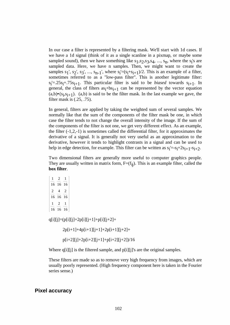
102

In our case a filter is represented by a filtering mask. We'll start with 1d cases. Ifwe have a 1d signal (think of it as a single scanline in a pixmap, or maybe somesampled sound), then we have something like s1,s2,s3,s4, ..., sn, where the si's aresampled data. Here, we have n samples. Then, we might want to create thesamples s1', s2', s3', ..., sn-1', where si'=(si+si+1)/2. This is an example of a filter,sometimes referred to as a "low-pass filter". This is another legitimate filter:si'=.25si+.75si+1. This particular filter is said to be biased towards si+1. Ingeneral, the class of filters asi+bsi+1 can be represented by the vector equation(a,b)• (si,si+1). (a,b) is said to be the filter mask. In the last example we gave, thefilter mask is (.25, .75).

In general, filters are applied by taking the weighted sum of several samples. Wenormally like that the sum of the components of the filter mask be one, in whichcase the filter tends to not change the overall intensity of the image. If the sum ofthe components of the filter is not one, we get very different effect. As an example,the filter (-1,2,-1) is sometimes called the differential filter, for it approximates thederivative of a signal. It is generally not very useful as an approximation to thederivative, however it tends to highlight contrasts in a signal and can be used tohelp in edge detection, for example. This filter can be written as si'=-si+2si+1-si+2.

Two dimensional filters are generally more useful to computer graphics people.They are usually written in matrix form, F=(fij ). This is an example filter, called thebox filter .

1

16

2

16

1

16

2

16

4

16

2

16

1

16

2

16

1

16

q[i][j]=(p[i][j]+2p[i][j+1]+p[i][j+2]+

2p[i+1]+4p[i+1][j+1]+2p[i+1][j+2]+

p[i+2][j]+2p[i+2][j+1]+p[i+2][j+2])/16

Where q[i][j] is the filtered sample, and p[i][j]'s are the original samples.

These filters are made so as to remove very high frequency from images, which areusually poorly represented. (High frequency component here is taken in the Fourierseries sense.)

Pixel accuracy

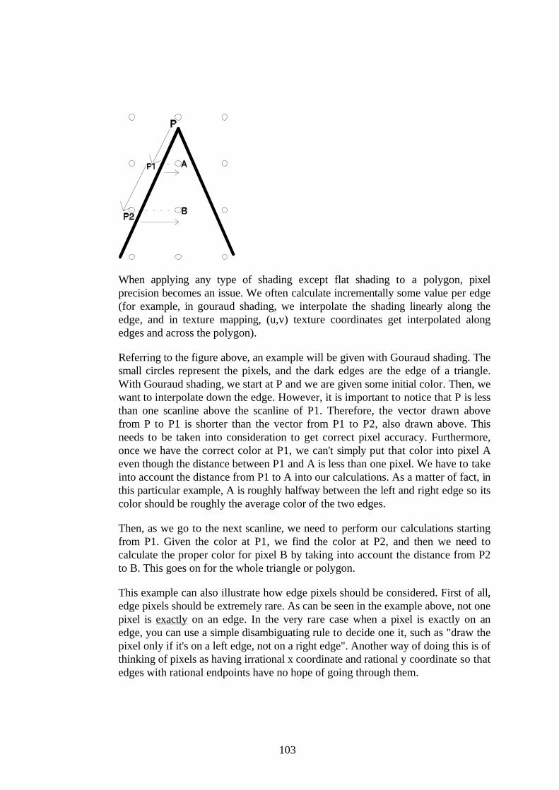
103

When applying any type of shading except flat shading to a polygon, pixelprecision becomes an issue. We often calculate incrementally some value per edge(for example, in gouraud shading, we interpolate the shading linearly along theedge, and in texture mapping, (u,v) texture coordinates get interpolated alongedges and across the polygon).

Referring to the figure above, an example will be given with Gouraud shading. Thesmall circles represent the pixels, and the dark edges are the edge of a triangle.With Gouraud shading, we start at P and we are given some initial color. Then, wewant to interpolate down the edge. However, it is important to notice that P is lessthan one scanline above the scanline of P1. Therefore, the vector drawn abovefrom P to P1 is shorter than the vector from P1 to P2, also drawn above. Thisneeds to be taken into consideration to get correct pixel accuracy. Furthermore,once we have the correct color at P1, we can't simply put that color into pixel Aeven though the distance between P1 and A is less than one pixel. We have to takeinto account the distance from P1 to A into our calculations. As a matter of fact, inthis particular example, A is roughly halfway between the left and right edge so itscolor should be roughly the average color of the two edges.

Then, as we go to the next scanline, we need to perform our calculations startingfrom P1. Given the color at P1, we find the color at P2, and then we need tocalculate the proper color for pixel B by taking into account the distance from P2to B. This goes on for the whole triangle or polygon.

This example can also illustrate how edge pixels should be considered. First of all,edge pixels should be extremely rare. As can be seen in the example above, not onepixel is exactly on an edge. In the very rare case when a pixel is exactly on anedge, you can use a simple disambiguating rule to decide one it, such as "draw thepixel only if it's on a left edge, not on a right edge". Another way of doing this is ofthinking of pixels as having irrational x coordinate and rational y coordinate so thatedges with rational endpoints have no hope of going through them.

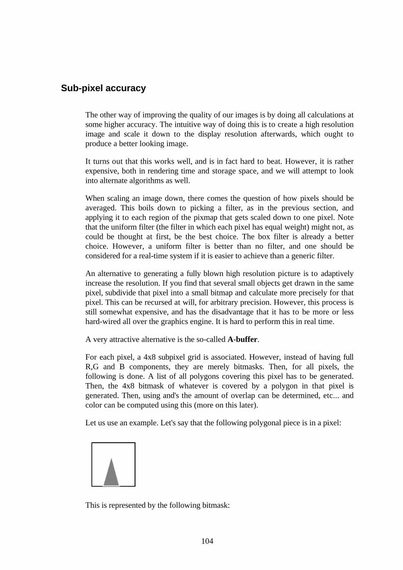
104

Sub-pixel accuracy

The other way of improving the quality of our images is by doing all calculations atsome higher accuracy. The intuitive way of doing this is to create a high resolutionimage and scale it down to the display resolution afterwards, which ought toproduce a better looking image.

It turns out that this works well, and is in fact hard to beat. However, it is ratherexpensive, both in rendering time and storage space, and we will attempt to lookinto alternate algorithms as well.

When scaling an image down, there comes the question of how pixels should beaveraged. This boils down to picking a filter, as in the previous section, andapplying it to each region of the pixmap that gets scaled down to one pixel. Notethat the uniform filter (the filter in which each pixel has equal weight) might not, ascould be thought at first, be the best choice. The box filter is already a betterchoice. However, a uniform filter is better than no filter, and one should beconsidered for a real-time system if it is easier to achieve than a generic filter.

An alternative to generating a fully blown high resolution picture is to adaptivelyincrease the resolution. If you find that several small objects get drawn in the samepixel, subdivide that pixel into a small bitmap and calculate more precisely for thatpixel. This can be recursed at will, for arbitrary precision. However, this process isstill somewhat expensive, and has the disadvantage that it has to be more or lesshard-wired all over the graphics engine. It is hard to perform this in real time.

A very attractive alternative is the so-called A-buffer .

For each pixel, a 4x8 subpixel grid is associated. However, instead of having fullR,G and B components, they are merely bitmasks. Then, for all pixels, thefollowing is done. A list of all polygons covering this pixel has to be generated.Then, the 4x8 bitmask of whatever is covered by a polygon in that pixel isgenerated. Then, using and's the amount of overlap can be determined, etc... andcolor can be computed using this (more on this later).

Let us use an example. Let's say that the following polygonal piece is in a pixel:

This is represented by the following bitmask:

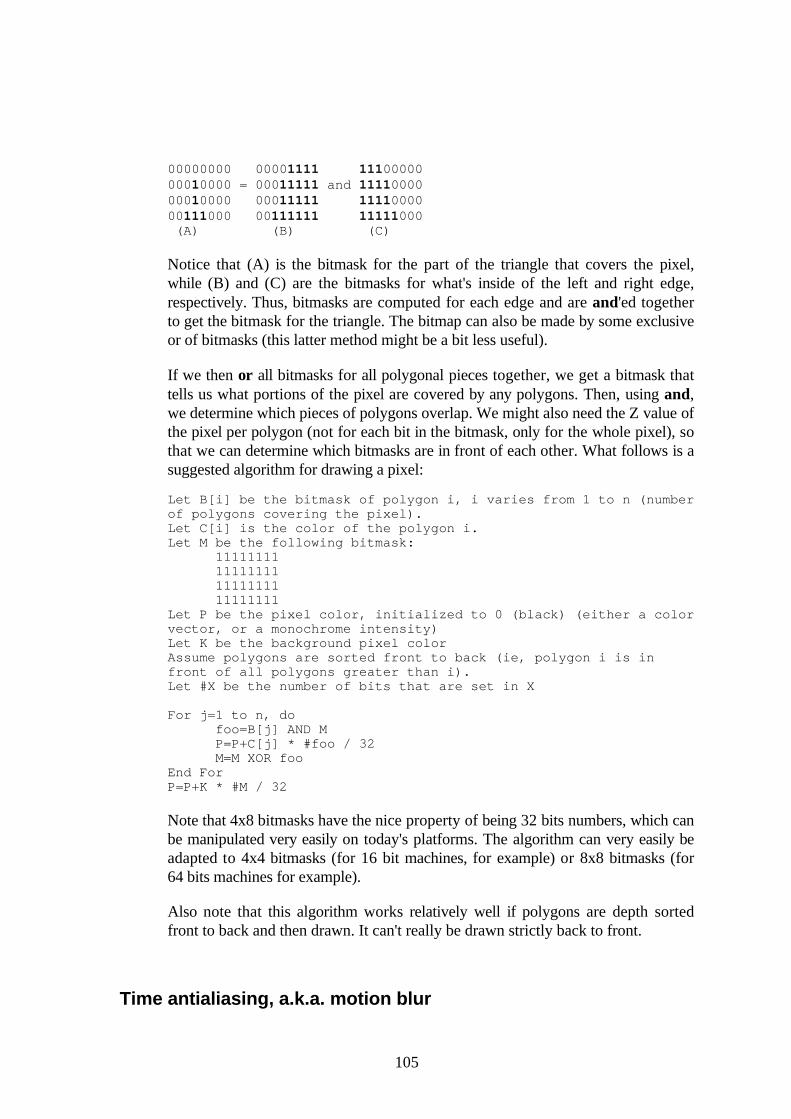
105

00000000 0000 1111 1110000000010000 = 000 11111 and 1111000000010000 000 11111 1111000000111000 00 111111 11111000 (A) (B) (C)

Notice that (A) is the bitmask for the part of the triangle that covers the pixel,while (B) and (C) are the bitmasks for what's inside of the left and right edge,respectively. Thus, bitmasks are computed for each edge and are and'ed togetherto get the bitmask for the triangle. The bitmap can also be made by some exclusiveor of bitmasks (this latter method might be a bit less useful).

If we then or all bitmasks for all polygonal pieces together, we get a bitmask thattells us what portions of the pixel are covered by any polygons. Then, using and,we determine which pieces of polygons overlap. We might also need the Z value ofthe pixel per polygon (not for each bit in the bitmask, only for the whole pixel), sothat we can determine which bitmasks are in front of each other. What follows is asuggested algorithm for drawing a pixel:

Let B[i] be the bitmask of polygon i, i varies from 1 to n (numberof polygons covering the pixel).Let C[i] is the color of the polygon i.Let M be the following bitmask:

11111111111111111111111111111111

Let P be the pixel color, initialized to 0 (black) (either a colorvector, or a monochrome intensity)Let K be the background pixel colorAssume polygons are sorted front to back (ie, polygon i is infront of all polygons greater than i).Let #X be the number of bits that are set in X

For j=1 to n, dofoo=B[j] AND MP=P+C[j] * #foo / 32M=M XOR foo

End ForP=P+K * #M / 32

Note that 4x8 bitmasks have the nice property of being 32 bits numbers, which canbe manipulated very easily on today's platforms. The algorithm can very easily beadapted to 4x4 bitmasks (for 16 bit machines, for example) or 8x8 bitmasks (for64 bits machines for example).

Also note that this algorithm works relatively well if polygons are depth sortedfront to back and then drawn. It can't really be drawn strictly back to front.

Time antialiasing, a.k.a. motion blur

106

We already mentioned the time aliasing effect. The most popular method ofperforming time antialiasing is still to generate several frames at very close intervaland merge them together. Once more, different filters can be applied.

One has to be careful when performing motion blur. Visible motion blur issomething that should only happen when things are moving faster than the framerate allows us to see. For example, an animation going at 24 fps (frames perseconds) should not have a trail behind an object moving one millimeter per frameon the screen. Put in different terms, an animation going at 24 fps should not showin a frame an event that happened 0.25 seconds ago. This effect, called persistence,can be quite annoying, and though it can produce an interesting result, it isgenerally not interesting or realistic to do so.

Therefore, if we want to generate a time antialiased animation at 24 fps, we reallyneed to generate something like an 120 fps animation, and then apply a filter tomerge the frames four by four and get a 24 fps animation. This is, as can be seen,quite expensive. However, it tends to produce very nice looking pictures. If theframe rate isn't kicked high enough, a fast moving object will appear (in ourexample above) as 4 distinct though semitransparent images per frame. This isprobably undesirable, but little can be done if objects are moving fast enough.

Other approaches have been attempted, mostly in raytracing, and will not bediscussed here. One notable area that might be worth further interest is theextruding of polygons as volumes in 4d with time as the fourth dimension andtrying to get the motion blur from that. This would have the advantage of beingmuch more exact than anything presented here, all the while not having problemswith very fast moving objects. However, even if the exact path of the object isknown, extrusion along that path might be too expensive or difficult to perform, solinear extrusion might have to be considered. Nevertheless, I suspect this wouldproduce very attractive results.

Mipmapping

107

Texture mapping was described previously. However, a naive approach was taken;we did not consider what happens when the texture is so scaled down that it takesseveral texels to cover a single pixel. In the context of this chapter, however, wewould like to somehow "average" (more properly, filter) the texels that cover asingle pixel to get a nicer looking picture. To illustrate the problem, if the textureis so shrunk that it barely covers one pixel, then the color of that pixel will be amore or less random point from the texture. Hence, if the texture is not very"smooth", this particular pixel can "blip", change color rapidly and scintillate. Thisis of course undesirable. Also, even though the texture seen from afar might beblue for the most part, a small reddish region might result in the whole pixelappearing red, which would be wrong.

Performing different approaches can be taken to this antialiasing problem. We canactually compute all the texels that fall within a pixel, then apply some filter,perhaps even based on the size of the texel in the pixel. These sort of approacheslend themselves very poorly to real-time applications, which is the main interest ofthis document, hence we will not approach them.

A real-time alternative is Mipmapping. The texture map is pre-filtered to differentdegrees, and at run time, we determine how much the texels get squished by theperspective transform, and the select the proper mipmap.

Uniform Mipmapping

Classically, this is how mipmapping is done. We start with a texture map. Say thetexture map is of size 64x64. Then, mipmaps of size 32x32, 16x16, 8x8, 4x4, 2x2and 1x1 are generated by recursively averaging 2x2 blocks of pixels. We start withthe 64x64 texture map, then average each 2x2 block to get a 32x32 mipmap. Thenwe filter that mipmap again to get a 16x16 mipmap, and so on. The mipmaps canbe labelled "mipmap #1" for the unfiltered texture map, "mipmap #2" for the firstmipmap, and so on.

The mipmap should be chosen based on the amount of squishing we think thetexels will undergo. If we feel that each pixel will cover about 4 texels (roughly a2x2 block), then we should use the 32x32 mipmap. If the texmap is even moresquished (perhaps 16 texels per pixel, 4x4) then the 16x16 mipmap should be used.

Let's look at memory requirements. Let K be the amount of memory used by thebasic texture map. First we observe that averaging 2x2 block of pixels and makingthe first mipmap makes something which takes one fourth as much memory as thetexture map. As a matter of fact, each time we generate another mipmap, thememory taken by the new mipmap is 1/4 that of the old. Hence the total memoryis:

K+K/4+K/16+K/64+K/256+...+K/(4n)<K+K/4+K/16+...+K/(4n)+...

108

=K(1+1/4+1/16+1/64+........)=4K/3

Hence, classical mipmapping takes but 1/3 more memory than straight texturemapping.

The problem of determining which mipmap to use is, however, not trivial. Asmentioned previously, this should be a function of the "squishing" undergone bythe texels. However, the squishing in the x direction can be vastly different fromthe squishing in the y direction. You can fight with this, or you can invent a newertype of mipmapping.

Nonuniform Mipmapping

Instead of scaling the texture map homogeneously (by the same factor in x and y),we can generate mipmaps with nonuniform scaling. This way, if there is a lot of"squishing" in a direction, but very little in the other, a relatively good mipmap canstill be found.

Still using the 64x64 example above, we would generate mipmaps of the followingsizes:

64x64 64x32 64x16 64x8 64x4 64x2 64x1

32x64 32x32 32x16 32x8 32x4 32x2 32x1

16x64 16x32 16x16 16x8 16x4 16x2 16x1

8x64 8x32 8x16 8x8 8x4 8x2 8x1

4x64 4x32 4x16 4x8 4x4 4x2 4x1

2x64 2x32 2x16 2x8 2x4 2x2 2x1

1x64 1x32 1x16 1x8 1x4 1x2 1x1

Note that the mipmaps can be indexed by a pair of number. For instance, themipmap 64x64 can be identified to the pair (1,1), the mipmap 64x16 could beidentified to the point (3,1), mipma 2x4 would be (5,6) and mipmap 1x1 would be(7,7).

It might appear on first look that this will require a lot of memory, however this isnot as bad as it might first appears. A geometric demonstration is given below.This figure contains the texture map plus all the mipmaps listed above. As can beseen, the memory taken by the mipmaps and the texture map is four times thememory taken by the texture map alone.

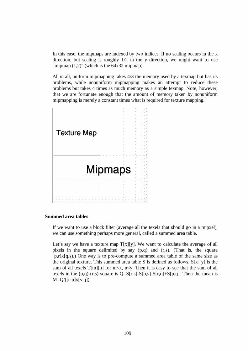
109

In this case, the mipmaps are indexed by two indices. If no scaling occurs in the xdirection, but scaling is roughly 1/2 in the y direction, we might want to use"mipmap (1,2)" (which is the 64x32 mipmap).

All in all, uniform mipmapping takes 4/3 the memory used by a texmap but has itsproblems, while nonuniform mipmapping makes an attempt to reduce theseproblems but takes 4 times as much memory as a simple texmap. Note, however,that we are fortunate enough that the amount of memory taken by nonuniformmipmapping is merely a constant times what is required for texture mapping.

Summed area tables

If we want to use a block filter (average all the texels that should go in a mipxel),we can use something perhaps more general, called a summed area table.

Let’s say we have a texture map T[x][y]. We want to calculate the average of allpixels in the square delimited by say (p,q) and (r,s). (That is, the square[p,r)x[q,s).) One way is to pre-compute a summed area table of the same size asthe original texture. This summed area table S is defined as follows. S[x][y] is thesum of all texels T[m][n] for m<x, n<y. Then it is easy to see that the sum of alltexels in the (p,q)-(r,s) square is Q=S[r,s]-S[p,s]-S[r,q]+S[p,q]. Then the mean isM=Q/([r-p]x[s-q]).

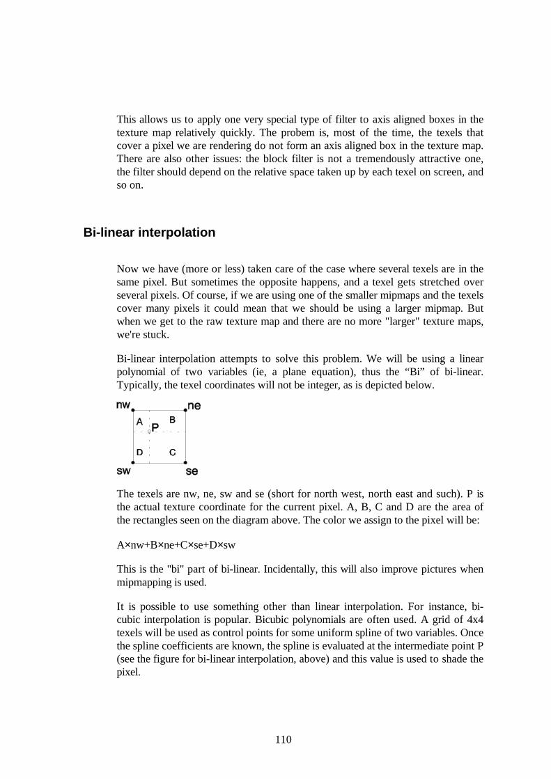
110

This allows us to apply one very special type of filter to axis aligned boxes in thetexture map relatively quickly. The probem is, most of the time, the texels thatcover a pixel we are rendering do not form an axis aligned box in the texture map.There are also other issues: the block filter is not a tremendously attractive one,the filter should depend on the relative space taken up by each texel on screen, andso on.

Bi-linear interpolation

Now we have (more or less) taken care of the case where several texels are in thesame pixel. But sometimes the opposite happens, and a texel gets stretched overseveral pixels. Of course, if we are using one of the smaller mipmaps and the texelscover many pixels it could mean that we should be using a larger mipmap. Butwhen we get to the raw texture map and there are no more "larger" texture maps,we're stuck.

Bi-linear interpolation attempts to solve this problem. We will be using a linearpolynomial of two variables (ie, a plane equation), thus the “Bi” of bi-linear.Typically, the texel coordinates will not be integer, as is depicted below.

The texels are nw, ne, sw and se (short for north west, north east and such). P isthe actual texture coordinate for the current pixel. A, B, C and D are the area ofthe rectangles seen on the diagram above. The color we assign to the pixel will be:

A×nw+B×ne+C×se+D×sw

This is the "bi" part of bi-linear. Incidentally, this will also improve pictures whenmipmapping is used.

It is possible to use something other than linear interpolation. For instance, bi-cubic interpolation is popular. Bicubic polynomials are often used. A grid of 4x4texels will be used as control points for some uniform spline of two variables. Oncethe spline coefficients are known, the spline is evaluated at the intermediate point P(see the figure for bi-linear interpolation, above) and this value is used to shade thepixel.

111

Tri-linear interpolation

Tri-linear interpolation is bi-linear interpolation with an additional interpolation.First, a description for uniform mipmapping will be given, then this will beextended to nonuniform mipmapping and summed area tables.

When we use mipmapping, we need a function which tells us what mipmap to use.However, maybe this function tells us to use "mipmap #3.15", which we round tosimply "mipmap #3". This means that we should use a mipmap somewhat inbetween 3 and 4, but more towards 3. Tri-linear interpolation simply interpolateslinearly the mipmap between mipmap 3 and 4 (probably using, in our specificexample of "mipmap #3.15", 85% of mipmap 3 and 15% of mipmap 4).

This will make the change in mipmaps quite smoother, which will have animportant effect on animations in particular.

Using nonuniform mipmapping, we simply extend our idea to interpolate linearlybetween four mipmaps. Ie, if we want mipmap #3.2 in the x direction and #5.7 inthe y direction, we mix in (0.8×0.3)=0.24 of mipmap (3,5) with (0.2×0.3)=0.06 ofmipmap (4,5), (0.8×0.7)=0.56 of mipmap (3,6) and lastly (0.2×0.7)=0.14 ofmipmap (4,7). As we can see, mipmap (3,6) is the dominant one, as is to beexpected and mipmap (4,5) is barely used at all.

112

Glossary

Complex numbers: a number with a real and imaginary part, of the form Z=a+bi, where i isthe imaginary part. We define i2=-1. This way, we can define addition,multiplication, subtraction, and even inverse. Complex numbers can be comparedto points in the plane. As such, they have a polar coordinate form. From this wecan define the euclidian norm, or absolute value of a complex number. By usingEuler's representation, we can put this form in exponential form. It is of note thatmultiplication by unit complex numbers represent rotations in the plane.

Convex: term used to describe polytopes, such as polygons and polyhedra. It means thatthe inside angle is always less than or equal to 180°. A triangle is always convex. Asquare or a rectangle is convex, but other quadrilaterals may not be convex. Theterm convex is sometimes used for a vertex or edge to say that the inside angle atthe vertex or edge is less than or equal to 180°. An equivalent definition ofconvexity is, given a polytope, the intersection of the polytope and any line isalways 0 or 2 points except in degenerate cases. A stricter mathematical definitionis used in the spline chapter. It is a generalization of our simpler definitions.

Concave: any non self-intersecting polytope that is not convex is concave.

Edge: a line segment between 2 vertices. An edge typically delimitates a polygon. Asquare has 4 edges, a cube has 12.

Euler angles: 3 angles used to represent a specific orientation. Can be used to representany rotation, but is not very useful in practice for several reasons. First, the orderin which the rotations are applied is important. Second, it is very hard to find theEuler angles for a given orientation. Third, the angles have very little physicalmeaning.

Face: a polygon that delimitates a polyhedron. A face is always planar. A cube has 6 faces.Also, since polygons in 3d have two sides, they are sometimes referred to as faces.

Mach banding: The human eye accentuates contrasts. Therefore, if two surfaces of slightlydifferent colors lie next to each other, the boundary between the two will be clearlyvisible since it's an area of high contrast (contrast is, more or less, change of colorover distance). This happens when we have too few colors to give a continuoustexture to a surface, or when coloring adjacent faces of an object with uniform butslightly different shades of the same color.

113

Matrix: a 2 dimensional array of real numbers. Can also be thought as an array of vectors,or a vector of vectors.

Normalizing: making a vector V of unit length, by multiplying it by 1/|V|.

Polygon: a flat, 2d polytope delimited by straight edges and vertices. Examples includetriangles, squares, decagons. We normally prefer all vertices to be distinct, and thatedges do not cross. We don't like it either when the polygon is disconnected (e.g.has several, distinct parts that are not connected).

Polyhedron: a 3d polytope delimited by planar faces, linear edges and vertices. Examplesinclude cubes, tetrahedra, icosahedra. As with the polygon, we prefer vertices tobe distinct, edges not to cross, faces not to intersect, and the polyhedron to bemade of one piece as opposed to several disconnected pieces.

Polynomial: a mathematical entity that can be reduced to the forma0+a1x+a2x2+a3x3+...+anxn for some n, ai being a real number and xi a realvariable. Example polynomials include: 3, 2+x, x5+2x+3, x(x+2)(x-3). Examplesof things that are not polynomials: x(x+1)/(x+2), x2+x+sinx.

Polytope: an object in n dimensions defined by linear constraints. Examples in 2d and 3dare polygons and polyhedra, respectively. Polytopes are normally made of a singlepiece. That is, from any point in a polytope, there is a path (which might betwisted) that can get you to any other point in the polytope without exiting thepolytope.

Quaternion: similar to a complex number, a quaternion has 1 real and 3 imaginary parts. Itis generally written as Q=a+bi+cj+dk, where i, j and k are orthonormal imaginaryparts. These imaginary components satisfy the following equalities: ij=-ij=k, jk=-jk=i, ki=-ik=j, i2=j2=k2=ijk=-1. From that, addition, subtraction and multiplicationoperations can be defined. The useful thing about quaternions is, just multiplicationby unit complex numbers represent rotations in 2d, multiplication by unitquaternions represent rotations in 3d.

Taylor series: A power series that approximates a function.

Texel: One unit in the texture map, the texture map equivalent of a pixel.

Texture mapping: Historically, this is the "sticking" of a "picture" on top of a polygon. Abitmap, called texture map, is mapped on a polygon or triangle. This has beengeneralized greatly however. Now, texture maps are sometimes replaced by afunction of an x,y,z point in space. Also, the texture need no longer be a simplepicture. The texture can be slight perturbations to the surface normal (bumpmapping), a "transparency level" (alpha channel) or a number of other things.

Pixel: The smallest dot displayable by the hardware. Also used to describe one smallsquare unit in a bitmap.

114

Vector: strictly speaking, a n-uplet, such as (3,2,5,1). It can be viewed as an arrow in anynumber of dimensions, from one point p1 to a point p2. The vector from (x,y,z) to(a,b,c) is (a-x,b-y,c-z).

Vertex: a point, usually called this way when it is the endpoint of at least one edge. Asquare has 4 vertices, a cube has 8.

115

Bibliography

[1] James Foley, Andries van Dam, Steven Feiner, John Hughes, Computer GraphicsPrinciples and Practice, Addison-Wesley, 1990.

[2] Thomas H. Cormen, Charles E. Leiserson, Ronald L. Rivest, Introduction toAlgorithms, McGraw-Hill, 1989.

[3] S. D. Conte, Carl de Boor, Elementary Numerical Analysis, McGraw-Hill, 1980.

[4] Ming Chieh Lin, Efficient Collision Detection for animation and robotics, PhDThesis at University of California at Berkeley, 1993.

[5] Barsky, B., Computer Graphics and Geometric Modeling Using Beta-splines,Springer-Verlag, New York, 1988.