Welcome to the course MAT3500/MAT4500 TOPOLOGY.My name is John Rognes, and my email address is rognes@math.uio.no.TOPOS τ oπoς means place/location. LOGOS λoγoς means study/reason. Topology

provides a language for proving results about shapes.Early examples in the work of Euler:Bridges of Konigsberg (1736). Seek continuous path traversing each bridge exactly once.

Distances immaterial. Reduces to a counting problem in graph theory, which is easier tosettle.

Euler characteristic (1758). The surface of a polyhedron consists of V vertices, E edges andF faces. The alternating sum χ = V −E+F is invariant under subdivision of the surface, andis in fact a topological invariant. Compare cube, cube with a truncated vertex, octahedron,and a toric solid. Suggests spheres/surfaces of convex bodies and tori are topologicallydistinct.

Topology emphasizes continuity, which ensures preservation of limits. Recall continuity inthe context of metric spaces, before generalizing to topological spaces.

Metric spaces (X, d) −→ Topological spaces (X, T ).Definition: A metric d on a set X is a (real-valued) function

d : X ×X −→ R(x, y) −→ d(x, y)

satisfying(a) d(x, y) ≥ 0 for all x, y ∈ X, and d(x, y) = 0 if and only if x = y.[We could have written d : X ×X → [0,∞) = R+.](b) d(x, y) = d(y, x) for all x, y ∈ X [symmetry].(c) d(x, z) ≤ d(x, y) + d(y, z) for all x, y, z ∈ X [triangle inequality].Draw a triangle 4xyz. We call the pair (X, d) a metric space. Elements of X are called

points.Example: X = Rn = {~x = (x1, . . . , xn) | xi ∈ R for 1 ≤ i ≤ n} with the Euclidean dis-

tance

d(~x, ~y) =√

(y1 − x1)2 + · · ·+ (yn − xn)2 =

(n∑i=1

(yi − xi)2

)1/2

.

Example: For a < b and p ≥ 1 real numbers, X = C([a, b]) = {f : [a, b] → R |f is continuous} with

dp(f, g) =

(∫ b

a

|g(t)− f(t)|p dt)1/p

the Lp-distance, equal to= ‖g − f‖p

given by the Lp-norm. The metric space (X, dp) comes from the normed vector space(X, ‖ − ‖p). In the case p = 2, the L2-norm

‖h‖2 = 〈h, h〉1/2

comes from the inner product

〈f, g〉 =

∫ b

a

f(t)g(t) dt

1

making (X, 〈−,−〉) an inner product space.Inner product spaces −→ normed vector spaces −→ metric spaces.Consider two metric spaces (X, dX) and (Y, dY ). A function f : X → Y is an isometry if

dX(x, y) = dY (f(x), f(y))

for all x, y ∈ X.Example: The isometries f : R→ R are the translations

f(x) = x+ b

and the reflections

f(x) = −x+ b .

These are isometric isomorphisms, meaning that f : X → Y is bijective, hence admits aninverse function g : Y → X, such that g(f(x)) = x for all x ∈ X and f(g(y)) = y for ally ∈ Y . We write g ◦ f = 1X and f ◦ g = 1Y . Note that g is automatically an isometry.

If there exists an isometric isomorphism f : (X, dX) → (Y, dY ) then (X, dX) and (Y, dY )are metrically equivalent. Any property about the points of X and their distances can betranslated to a logically equivalent statement about the points of Y and their distances, bysending each x ∈ X to its image f(x) ∈ Y .

The study of metric spaces up to metric equivalence may (somewhat superfluously) becalled metric geometry. Trigonometry is a simple example. Euler’s studies do not dependon the full metric structure.

GEOMETRY means earth measurement.Topology focuses on a less rigid class of functions, namely the continuous functions, briefly

called maps.Definition: Let (X, dX) and (Y, dY ) be two metric spaces, and let f : X → Y be a function.

Fix a point x ∈ X. We say that f is continuous at x if for any positive real number ε thereis a positive real number δ such that for each y ∈ X with dX(x, y) < δ it is true thatdY (f(x), f(y)) < ε. “In order to surely be mapped within ε of f(x) in Y , it is enough tostart within δ of x in X.”

If f : X → Y is continuous at x, for each point x ∈ X, we say that f is continuous, orthat f is a map.

Here are some sample results about continuous functions f : [a, b]→ R.Theorem: f achieves its minimum c and its maximum d [extreme value theorem].This ensures that optimization problems have a solution.Theorem: f achieves all values between c and d [intermediate value theorem].Corollary: If f : [0, 1] → [0, 1] is continuous, then there exists a point x ∈ [0, 1] with

f(x) = x, i.e., a fixed point.Proof: Consider g : [0, 1]→ R given by g(x) = f(x)− x. Then g(0) ≥ 0 and g(1) ≤ 0, so

g(x) = 0 for some x ∈ [0, 1]. QEDWe will extend these kinds of results to all metric spaces (X, d), and beyond, to topological

spaces (X, T ).The ε-δ definition of continuity can we reformulated in terms of the notion of open subsets.

We first review this for metric spaces, and then turn this into a definition of topologicalspaces.

2

Definition: Let (X, d) be a metric space, x ∈ X a point and ε > 0 a positive real number.Let

Bd(x, ε) = {y ∈ X | d(x, y) < ε}be the (open) ε-ball around x in X. We simply write B(x, ε) if d is implicit.

A subset U of X is open if for each point x ∈ U there is an ε > 0 such that B(x, ε) ⊂ U .Example: An open interval (a, b) in R is open, but a half-open interval (a, b] or [a, b), or

a closed interval [a, b], is not. Note: To be ‘not open’ is not the same as being ‘closed’.Lemma: An ε-ball U = B(x, ε) is open.Proof: For each y ∈ B(x, ε) we must find a δ > 0 such that B(y, δ) ⊂ B(x, ε). Let

δ = ε− d(x, y). Then for each z ∈ B(y, δ) we have d(x, z) ≤ d(x, y) + d(y, z) < d(x, y) + δ =d(x, y) + ε− d(x, y) = ε. QED

Proposition: Let (X, dX) and (Y, dY ) be metric spaces, and let f : X → Y be a function.Then f is continuous if and only if for each open subset V ⊂ Y the preimage

f−1(V ) = {x ∈ X | f(x) ∈ V }is open in X.

Moral: Continuity of f : (X, dX) → (Y, dY ) only depends on which subsets of X and Yare open, not on the precise metrics dX and dY .

Basic properties of open subsets in (X, d):Proposition: Let (X, d) be a metric space.(a) The empty and full subsets U = ∅ and U = X are open.(b) If U1, . . . , Un are open subsets in X, then the finite intersection

U1 ∩ · · · ∩ Un =n⋂i=1

Ui

is also open in X.(c) If Uα, Uβ, . . . is any collection of open subsets in X, where α, β, · · · ∈ J lie in any

indexing set, then the union

Uα ∪ Uβ ∪ · · · =⋃α∈J

Uα

is also open in X.Proof: ((ETC))

§12 Topological Spaces: In point set topology we interpret shape to mean a set X, whoseelements we call the points of X, together with enough information to determine whichfunctions mapping to or from X are continuous. This means that we must know exactlywhich subsets U ⊂ X are open. We do this by axiomatically declaring some or all of thesubsets to be open. The remaining subsets are then not open. To obtain a reasonabletheory, we insist that the specification of which subsets of X are open must satisfy the threeconditions of the proposition above.

Definition: A topological space is a set X together with a specification of which subsetsU ⊂ X are said to be open. We assume that

(a) The subsets ∅ and X are open.(b) The intersection

U1 ∩ · · · ∩ Unof any finite collection {U1, . . . , Un} of open subsets of X is open.

3

(c) The union ⋃α∈J

Uα

of any (finite or infinite) collection {Uα}α∈J of open subsets of X is open.Remark: The ordering of (b) and (c) is often switched. We think finite intersections are

easier than arbitrary unions. By induction on n it suffices to check (b) for n = 2. The casesn = 1 and J = {α} (a single element) are tautological. The case J = ∅ of (c) amounts tothe case U = ∅ of (a), while the case n = 0 of (b) can be interpreted as the case U = X of(a).]

Example: A metric space (X, d) determines a topological space, with the same set X ofpoints, where we declare a subset U ⊂ X to be open in the topological sense if and only ifit is open in the metric sense. We call this the topological space underlying the given metricspace.

Consider a topological space X, defined as above. We need notation for the specificationof which subsets U of X are open, and which are not. We do this by letting

T = {U | U is an open subset of X}denote the collection of all open subsets. This is a set whose elements are the sets U thatare open subsets of X, i.e., T is a set of sets. To avoid confusion, we will refer to a set ofsets as a collection of sets, so that a collection is a set whose elements are themselves sets.Knowledge of the collection T then determines which subsets of X are open, since U ⊂ Xis open if and only if U ∈ T . We reformulate the definition as follows:

Definition: A topological space (X, T ) is a set X and a collection T of subsets of X, suchthat

(a) ∅ ∈ T and X ∈ T .(b) If U1, . . . , Un ∈ T then U1 ∩ · · · ∩ Un ∈ T .(c) If Uα ∈ T for each α ∈ J , then

⋃α∈J Uα ∈ T .

We call the elements x ∈ X the points of X, and we call the elements U ∈ T the opensubsets of X. We call the collection T the topology on X.

Example: Let X be any set. In the trivial topology on X only ∅ and X are open subsets,so that

Ttriv = {∅, X} .Example: Let X be any set. In the discrete topology on X every subset U ⊂ X is open,

so thatTdisc = {U | U ⊂ X} = P(X)

equals the power set on X.Example: The empty space X = ∅ admits only one topology, which is both trivial and

discrete:Ttriv = Tdisc = {∅} .

Example: Each one point space X = {a} also admits only one topology, which is bothtrivial and discrete:

Ttriv = Tdisc = {∅, X} .Example: A two point space X = {a, b} admits four different topologies.(1) The trivial topology Ttriv = {∅, X}.(2) A Sierpinski topology Ta = {∅, {a}, X} where {a} is open but {b} is not.

4

(3) Another Sierpinski topology Tb = {∅, {b}, X} where {b} is open but {a} is not.(4) The discrete topology Tdisc = {∅, {a}, {b}, X}.Example: A three point space X = {a, b, c} admits 29 different topologies. We omit to list

them.Definition: Let (X, TX) and (Y, TY ) be topological spaces, and let f : X → Y be a function.

Then f is continuous if for each open subset V in Y the preimage

f−1(V ) = {x ∈ X | f(x) ∈ V }is open in X.

Equivalently, f is continuous if for each V ∈ TY the preimage f−1(V ) ∈ TX .[In terms of power sets, continuity asks that the function V 7→ f−1(V ) takes TY ⊂ P(Y )

to TX ⊂ P(X).]If (X, dX) and (Y, dY ) are metric spaces, with underlying topological spaces (X, TX) and

(Y, TY ), then a function f : X → Y is continuous in the metric sense if and only if it iscontinuous in the topological sense. Hence continuity of f : X → Y only depends on thetopological spaces (X, TX) and (Y, TY ), not on the specific metrics dX and dY .

For metric spaces, we can talk about isometries (for metric geometry) or continuous maps(for topology), while for topological spaces we can (only) talk about continuous maps. How-ever, for these, the topological spaces are more closely adapted to the essence of that notion.

Different metric spaces can have the same underlying topological space. Since the pointsets are the same, this means that two metric spaces (X, d1) and (X, d2), with differentmetrics d1 and d2, can have the same notion of open subset, and hence determine the sametopology T and underlying topological space (X, T ).

Consider the unit circle

X = S1 = {(x1, x2) | x21 + x2

2 = 1} ⊂ R2

in the Euclidean plane. We can give S1 the subspace metric d1, where

d1(~x, ~y) = ‖~y − ~x‖2

for ~x, ~y ∈ S1 equals the distance between these points in R2, i.e., the length of the chordconnecting them.

We can also give S1 the Riemannian metric d2, where

d2(~x, ~y) = inf ‖γ‖is the length of the shortest path γ in S1 connecting ~x to ~y, i.e., the length of the arcconnecting the two points. If γ : [a, b] → S1 ⊂ R is a continuously differentiable path, itslength is defined as

‖γ‖ =

∫ b

a

‖γ′(t)‖2 dt ,

where γ′(t) ∈ R2 gives the velocity and ‖γ′(t)‖2 gives the speed of the curve at time t.These metrics differ, but give rise to the same open subsets. This follows from

d1(~x, ~y)

2= sin

d2(~x, ~y)

2.

Fortunately, even if we people may disagree on what is the correct measure of distancebetween two points on S1, we will agree on what it means for functions f : S1 → Y org : W → S1 to be continuous, for either one of these two metrics.

5

In the analogous situation for the unit sphere S2 ⊂ R3, modeling the Earth’s surface,moving one Earth radius from the North pole with respect to the subspace metric from R3

brings you to 30 degrees north of the equator, near Cairo, while moving one Earth radiuswith respect to the Riemannian metric only brings you to 32.7 degrees north, near Nazareth.

The rule (Metric spaces −→ Topological spaces) is thus not one-to-one (= injective), andloses some information, but this information is irrelevant for the purpose of understandingcontinuity.

The passage to topological spaces also permits us to generalize the theory and considernew examples, because not every topological space comes from a metric space.

Example: In any metric space (X, d), distinct points x 6= y can be separated by disjointopen subsets U = B(x, ε) and V = B(y, ε), where we set ε = d(x, y)/2. This is calledthe Hausdorff property. However, not every topological space has the Hausdorff property.For example, this happens for the trivial topology and the two Sierpinski topologies onX = {a, b}. Hence these topological spaces cannot come from a metric space, and are notmetrizable.

A less obscure topology that does not come from a metric is the topology Tp of pointwiseconvergence on X = C([a, b]). Each topology determines a notion of convergence, and forTp a sequence of functions

f1, f2, . . . , fn, . . .

converges in (X, Tp) to a function g if and only if the sequence of real numbers

f1(t), f2(t), . . . , fn(t), . . .

converges in R to g(t), for each t ∈ [a, b]. This is a sensible topology on X, and it has theHausdorff property, but it does nonetheless not come from a metric d on X = C([a, b]).

The rule (Metric spaces −→ Topological spaces) is thus also not onto (= surjective). Toview pointwise convergence as an instance of a general notion of convergence, we must gobeyond metric spaces.

We will study the Urysohn/Tychonoff metrization theorem, which gives sufficient (but notnecessary) conditions for a topological space to come from a metric space.

We shall define what it means for a topological space (X, TX) to be compact. A subsetA ⊂ R, with the subspace topology is compact if and only if it is closed and bounded, inthe metric sense. In particular, a closed interval [a, b] is compact. Moreover, the continuousimage of a compact space is compact. Hence, if f : [a, b] → R is continuous, then its imageA = f([a, b]) is a closed and bounded subset of R. In particular, c = inf A and d = supAare both elements of A, which implies that f achieves its minimum and its maximum. Thegeneral notion of compactness, and the theorem that the continuous image of a compactspace is compact, vastly generalize the extreme value theorem.

We shall also define what it means for a topological space (X, TX) to be connected. Asubset A ⊂ R is connected if and only if it is an interval. In particular, a closed interval [a, b]is connected. Moreover, the continuous image of a connected space is connected. Hence, iff : [a, b] → R is continuous, then its image A = f([a, b]) ⊂ [c, d] is an interval in R, hencemust be equal to [c, d]. In particular, each intermediate value between c and d is also achievedby f . The general notion of connectedness, and the theorem that the continuous image of aconnected space is connected, vastly generalize the intermediate value theorem.

The union [0, 1] ∪ [2, 3] is compact but not connected. The interval [1,∞) is connectedbut not compact.

6

Theorem: If f : [0, 1] × [0, 1] → [0, 1] × [0, 1] is any continuous map, then there exists afixed point ~x = (x1, x2) ∈ [0, 1]× [0, 1] with f(~x) = ~x.

We prove this in Section 55, using the fundamental group. More generally, Brouwer proved:Theorem: If f : [0, 1]n → [0, 1]n is any continuous map, then there exists a fixed point

~x ∈ [0, 1]n with f(~x) = ~x.The proof for n ≥ 3 uses homology, discussed in MAT4530 – Algebraic Topology I.

Two topological spaces (X, TX) and (Y, TY ) are topologically equivalent, if there existsmutually inverse continuous functions f : X → Y and g : Y → X. We then call f (or g) ahomeomorphism, and say that X and Y are homeomorphic. We often write X ∼= Y or

f : X∼=−→ Y

to indicate that f is a homeomorphism.HOMEO means similar.Example: If X = (0, 1] and Y = [1,∞), the functions f : X → Y with f(x) = 1/x and

g : Y → X with g(y) = 1/y are mutually inverse and both continuous. Hence f : (0, 1] →[1,∞) is a homeomorphism.

In general, a homeomorphism f and its inverse g specify a one-to-one correspondence (=bijection) between the points of X and the points of Y , sending x ∈ X to f(x) ∈ Y . Underthis correspondence, a subset U ⊂ X is open if and only if

f(U) = {f(x) ∈ Y | x ∈ U}is open in Y . Note that this is equal to the set

g−1(U) = {y ∈ Y | g(y) ∈ U} .Hence any statement about (X, TX) that only refers to the points and open subsets of Xis logically equivalent to the corresponding statement about (Y, TY ), under the substitutionx 7→ f(x), U 7→ f(U) = g−1(U). Properties given by such statements are said to betopological properties.

For example, for a space to be discrete, Hausdorff, metrizable, compact or connected, areall examples of topological properties.

The surface of a doughnut, the surface of a mug with one handle, the space of possibleplacements for the hour hand and the minute hand of an analog clock, the space of config-urations for a suitable linkage, the product space S1 × S1, a quotient space of the squareI × I, a quotient space of a hexagon, and the complex points on an elliptic curve, are allexamples of topologically equivalent spaces. These are all Hausdorff, metrizable, compactand connected, but are not discrete.

—Metric properties. Completeness and completion. Metrics on the rational numbers. The

reals and the p-adic numbers. Product relation. The functional equation for the Riemannζ-function (in Landau ξ-form).

Sequential spaces, compactly generated (weak) Hausdorff spaces.Grothendieck topoi, quasi-topological spaces.Local vs. global. Manifold geometry. Topological, PL, differentiable, (complex) analytic,

algebraic categories. Singularities.Projective spaces. Zariski topology.—

7

§13 Bases for Topologies: Explicitly specifying a topology T can be cumbersome.Example: For X = R with the metric topology, the open subsets U ⊂ X are (finite or)

countable unions of disjoint open intervals:

U =∐i

(ai, bi) .

For X = R2 with the metric topology, an explicit enumeration of the open subsets (withoutrepetitions) is difficult to spell out.

In the case of metric spaces (X, d), the ε-balls B(x, ε) help us present open sets.Lemma: Each open U ⊂ X is a union of ε-balls (for varying x ∈ X and ε > 0), and each

such union is open.Proof: Let U be (metrically) open. For each x ∈ U choose εx > 0 such that B(x, εx) ⊂ U .

Then

U =⋃x∈U

B(x, εx) .

QEDHence the metrically open subsets of X are precisely the unions of (arbitrary collections

of) ε-balls. They key feature of ε-balls that ensures that the metrically open sets define atopology is the following.

Lemma: Let B1 = B(x1, ε1) and B2 = B(x2, ε2) be any two ε-balls. For each x ∈ B1 ∩B2

there is an εx > 0 such that

B(x, εx) ⊂ B1 ∩B2 .

Equivalently, the intersection B1 ∩B2 is a union of ε-balls.Proof: Let

εx = min{ε1 − d(x1, x), ε2 − d(x2, x)} .Then y ∈ B(x, εx) satisfies d(x1, y) ≤ d(x1, x) + d(x, y) < d(x1, x) + ε1 − d(x1, x) = ε1, soy ∈ B1. Likewise y ∈ B2. Hence

B1 ∩B2 =⋃

x∈B1∩B2

B(x, εx) .

QEDWe carry these ideas over to general topological spaces. Let X be any set.Definition: A collection B of subsets of X is called a basis if(a) for each x ∈ X there is a basis element B ∈ B with x ∈ B, and(b) for any two basis elements B1, B2 ∈ B and any x ∈ B1 ∩B2 there is a Bx ∈ B with

x ∈ Bx ⊂ B1 ∩B2 .

Lemma: Condition (b) is equivalent to asking that the intersection of any two basiselements is a union

B1 ∩B2 =⋃α∈J

Bα

of basis elements.Proof: For each x ∈ B1 ∩B2 choose Bx as in (b). Then

B1 ∩B2 =⋃

x∈B1∩B2

Bx .

8

QEDDefinition: A basis B generates a topology T , with open subsets given by arbitrary unions

U =⋃α∈J

Bα

of basis elements Bα ∈ B.Lemma 13.1’: A subset U ⊂ X is open if and only if for each x ∈ U there exists a basis

element B ∈ B with

x ∈ B ⊂ U .

Proof: If

U =⋃α∈J

Bα

is open, and x ∈ U , then there exists an α with

x ∈ Bα ⊂ U

and Bα ∈ B. Conversely, if we for each x ∈ U can choose a Bx ∈ B with x ∈ Bx ⊂ U then

U =⋃x∈U

Bx

is a union of basis elements, hence is open. QEDWe must justify the term “topology”.Lemma: The collection T is a topology on X.Proof: (a) The empty subset U = ∅ is the union over J = ∅. The full subset U = X is

the union over J = X, where Bx ∈ B is any basis element containing x.(b) If U =

⋃α∈J Bα and V =

⋃β∈K Bβ are open, with each Bα, Bβ ∈ B, then

U ∩ V =⋃

α∈J,β∈K

Bα ∩Bβ

is a union of intersections Bα ∩Bβ, each of which is a union of basis elements. Hence U ∩ Vis a union of basis elements, and is open.

(c) Any union of unions of basis elements is a union of basis elements, hence is open. QEDIn this situation, we say that B is a basis for the topology T . This is similar, but not

identical, to the notion of a basis for a vector space. In a vector space, each vector can beuniquely written as a finite linear combination of basis vectors. In a topological space, eachopen subset can be written as a union of basis elements. However, the presentation is notassumed to be unique, and the union may well be over an infinite indexing set. In bothsituations, the choice of a basis is hardly ever unique, so different bases can generated thesame topology.

Example: In a metric space (X, d), the ε-balls

B = {B(x, ε) | x ∈ X, ε > 0}form a basis for the metric topology T .

Example: The open intervals

(a, b) = {x ∈ R | a < x < b}form a basis for the metric topology on R.

9

Example: Circular disc Bcirc and rectangular Brect bases for topologies on R2.

(a, b)× (c, d) ∩ (a′, b′)× (c′, d′) = (a′, b)× (c′, d)

if a ≤ a′ < b ≤ b′, c ≤ c′ < d ≤ d′.Example: The single set X forms a basis for the trivial topology on X.Example: The singleton sets {x} for x ∈ X form a basis for the discrete topology on X.How can we recognize that a collection C is a basis for a given topology T ?Lemma 13.2: Let (X, T ) be a topological space, and let C be a collection of open subsets

in X. Suppose that for each open U ⊂ X and each point x ∈ U there is a C ∈ C withx ∈ C ⊂ U . Then C is a basis for the topology T .

Proof: (1) Check that C is a basis. (2) Check that the topology T ′ generated by C is equalto T . ((ETC))

Coarser and finer topologies:When X has two or more elements, there exist several different topologies on X. Some of

these are comparable in the following sense. If T ′ and T are topologies on the same set X,we say that T ′ is finer than T if T ′ ⊃ T , i.e., if each open subset in (X, T ) is also open in(X, T ′). We then also say that T is coarser than T ′.

Example: The discrete topology is finer than any other topology. The trivial topologyis coarser than any other topology. The Sierpinski topology Ta is not comparable with theSierpinski topology Tb.

Clearly B ⊂ T .Lemma: The topology T generated by a basis B is the coarsest topology that contains B.Lemma 13.3: Let B and B′ be bases for the topologies T and T ′ respectively, on X. The

following are equivalent:(1) The topology T ′ is finer than the topology T .(2) For each point x ∈ X and basis element B ∈ B with x ∈ B there is a basis element

B′ ∈ B′ with

x ∈ B′ ⊂ B .

Proof: ((ETC))Example: The circular disc basis B = Bcirc and the rectangular basis B′ = Brect define the

same topology, T = T ′, on R2.Definition: For any set X, the identity function id = idX : X → X is given by id(x) = x

for each x ∈ X.Lemma: Let T1 and T2 be topologies on X. The identity function idX : (X, T1)→ (X, T2)

is continuous if and only if T1 is finer than T2.Proof: Continuity asks that for each V ∈ T2 the preimage

id−1X (V ) = V

lies in T1, i.e., that T2 ⊂ T1.Roughly speaking, continuous functions map from finer to coarser topologies. Functions

going the other way, from coarser to finer topologies, are usually discontinuous.Subbases:We obtain a topology from a basis by imposing closure under arbitrary unions. We can

obtain a basis from a smaller collection, called a subbasis, by imposing closure under finiteintersections.

10

Definition: A subbasis S is any collection of subsets of X. The basis B generated by S isthe collection of finite intersections

B = S1 ∩ · · · ∩ Snof subbasis elements S1, . . . , Sn ∈ S. The topology T generated by the subbasis S is thetopology generated by this basis. It consists of arbitrary unions of finite intersections ofsubbasis elements.

Lemma: The collection B is a basis.Proof: (a) The empty intersection of subset of X (with n = 0) is X, so X ∈ B.(b) The intersection of two basis elements B1 = S1 ∩ · · · ∩ Sn and B2 = Sn+1 ∩ · · · ∩ Sn+m

is the basis element

B1 ∩B2 = S1 ∩ · · · ∩ Sn+m .

QEDMunkres assumes that for each x ∈ X there is some S ∈ S with x ∈ S. This appears to

be superfluous. Clearly S ⊂ B ⊂ T .Lemma: The topology T generated by S is the coarsest topology that contains S.We will see examples of subbases when we discuss product topologies in Section 15. The

following example appears in Section 46.Example: A subbasis for the topology of pointwise convergence Tp on X = C([a, b]) is the

collection of subsets

St,(c,d) = {f : [a, b]→ R | f(t) ∈ (c, d)} ,where t ∈ [a, b] and (c, d) ⊂ R.

Continuity in terms of bases and subbases in the target:Lemma: Let (X, TX) and (Y, TY ) be topological spaces, and let B be a basis for the

topology on Y . A function f : X → Y is continuous if and only if for each basis elementB ∈ B the preimage f−1(B) is open in X.

Proof: Each open subset in Y is a union

V =⋃α∈J

Bα

of basis elements Bα ∈ B, and

f−1(V ) =⋃α∈J

f−1(Bα) ,

so f−1(V ) is open if each f−1(Bα) is open in X.Example: If (Y, d) is a metric space, a function f : X → Y is continuous if and only if the

preimage

f−1(Bd(y, ε))

of each ε-ball in (Y, d) is open in X.Lemma: Let (X, TX) and (Y, TY ) be topological spaces, and let S be a subbasis for the

topology on Y . A function f : X → Y is continuous if and only if for each subbasis elementS ∈ S the preimage f−1(S) is open in X.

Proof: Let B be the basis generated by S. Each basis element is a finite intersection

B = S1 ∩ · · · ∩ Sn11

of subbasis elements Si ∈ S, and

f−1(B) = f−1(S1) ∩ · · · ∩ f−1(Sn) ,

so f−1(B) is open if each f−1(Si) is open in X. Now use the previous lemma.

§15 The Product Topology on X × Y : If X and Y are sets, the Cartesian product

X × Y = {(x, y) | x ∈ X, y ∈ Y }is the set of ordered pairs (x, y), with x in X and y ∈ Y .

Example: R2 = R× R is the Cartesian plane.Let Z be any set. To give a function

f : Z −→ X × Yis equivalent to give two functions g : Z → X and h : Z → Y , related by

f(z) = (g(z), h(z))

for each z ∈ Z. If X, Y and Z are topological spaces, we will now give the set X × Ya topology, so that the function f is continuous if and only if the functions g and h arecontinuous. To give a map

f : Z −→ X × Ywill thus be equivalent to give two maps g : Z → X and h : Z → Y , related by

f(z) = (g(z), h(z))

for each z ∈ Z. This so-called universal property characterizes the product topology onX × Y , and could be taken as a definition, once one knows that such a topology exists.

Definition: Let (X, TX) and (Y, TY ) be topological spaces. The product basis on X × Y isthe collection

B = {U × V | U ∈ TX , V ∈ TY }of subsets of X × Y . The product topology T on X × Y is the topology generated by B.

((Draw picture of U × V ⊂ X × Y .))We check that B is a basis (for a topology) on X × Y . (a) Since X ∈ TX and Y ∈ TY we

have X × Y ∈ B, so each (x, y) ∈ X × Y lies in a basis element. (b) Let B1 = U1 × V1 andB2 = U2 × V2 be basis elements. Then

B1 ∩B2 = (U1 ∩ U2)× (V1 ∩ V2)

is also a basis element, since U1 ∩ U2 ∈ TX and V1 ∩ V2 ∈ TY .The union of two product basis elements

(U1 × V1) ∪ (U2 × V2)

is usually not a basis element. The product basis B is therefore usually not a topology. Thetopology it generates instead consists of arbitrary unions

W =⋃α∈J

Uα × Vα

of basis elements.Proposition (= Theorem 15.1): Let B be a basis for a topology on X, and let C be a basis

for a topology on Y . Then the collection

D = {B × C | B ∈ B, C ∈ C}12

is a basis for the product topology on X × Y .Proof: Apply the recognition Lemma 13.2. For each openW ⊂ X×Y and point (x, y) ∈ W

we need to find a D ∈ D with (x, y) ∈ D ⊂ W . Since W is open, there is a product basiselement U × V with (x, y) ∈ U × V ⊂ W , where U is open in X and Y is open in V . Thenx ∈ U and y ∈ V . Since U is open, there is a basis element B ∈ B with x ∈ B ⊂ U . Likewisethere is a basis element C ∈ C with y ∈ C ⊂ V . Then D = B × C is as required. QED

Example: The open rectangles(a, b)× (c, d)

form a basis for the product topology on R2 = R× R. This equals the “rectangular” basis.We have seen that this defines the same topology as the “circular” or “metric” basis withelements

B((x, y), ε)

where (x, y) ∈ R2 and ε > 0. Hence the product topology and the metric topology on R2

are the same.Example: S1×S1 with the product topology is the torus surface. (This is not homeomor-

phic to the unit sphere S2.)The product basis comes from a smaller subbasis. This point of view will be useful when

we consider products of an arbitrary collection of topological spaces.Definition: Let (X, TX) and (Y, TY ) be topological spaces. The product subbasis on X×Y

is the collectionS = {U × Y | U ∈ TX} ∪ {X × V | V ∈ TY }

of subsets of X × Y .Lemma: The product subbasis S generates the product basis B, hence also the product

topology T , on X × Y .Proof: Finite intersections of subbasis elements are all of the form

(U × Y ) ∩ (X × V ) = U ∩ Vwith U ⊂ X and V ⊂ Y open. Hence S generates the product basis B. QED

Let

π1 : X × Y −→ X

(x, y) 7−→ x

be the projection to the first coordinate, and let

π2 : X × Y −→ Y

(x, y) 7−→ y

be the projection to the second coordinate.Lemma: Give X × Y the product topology. Then the projections

π1 : X × Y −→ X

andπ2 : X × Y −→ Y

are continuous.Proof: For each open U ⊂ X the preimage

π−11 (U) = U × Y

13

lies in the product (sub-)basis, hence is open in the product topology. Likewise, for eachopen V ⊂ Y the preimage

π−12 (V ) = X × V

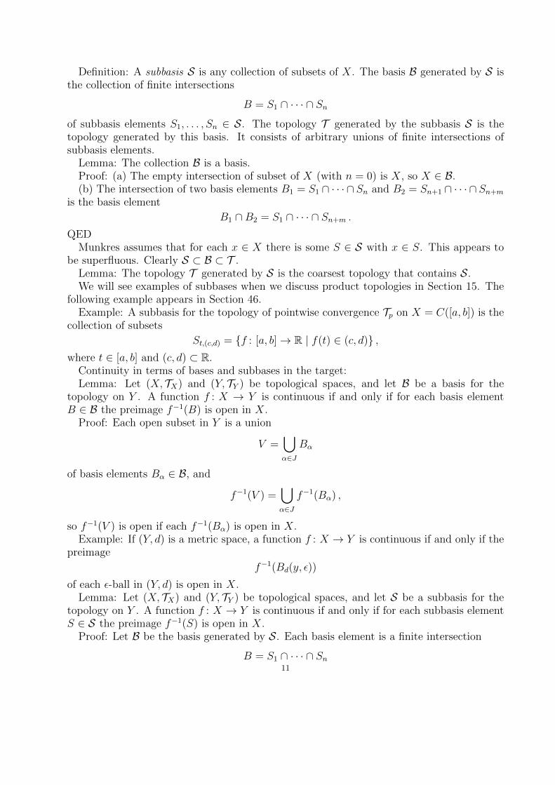
lies in the product (sub-)basis, hence is open in the product topology. QEDWe can now verify the universal property of the product topology.Proposition: Let Z, X and Y be topological spaces, and give X×Y the product topology.

A functionf : Z −→ X × Y

is continuous if and only if its component functions

g = π1f : Z −→ X

andh = π2f : Z −→ Y

are both continuous.Z

π1f

{{f

��

π2f

##X X × Yπ1oo

π2// Y

Proof: We can check continuity of f using the product subbasis

S = {π−11 (U) | U ∈ TX} ∪ {π−1

2 (V ) | V ∈ TY } .Hence f is a map if and only if

f−1(π−11 (U)) = g−1(U)

is open in Z for each open U ⊂ X, and

f−1(π−12 (V )) = h−1(V )

is open in Z for each open V ⊂ Y . This is equivalent to g and h being continuous. QED

§16 The Subspace Topology on Y ⊂ X: Let Y be a subset of X. Let Z be any set. Togive a function

f : Z −→ Y

is equivalent to giving a function g : Z → X with g(z) ∈ Y for each z ∈ Z. If X and Zare topological spaces, we will now give the subset Y a topology such that the function f iscontinuous if and only if g is continuous.

Definition: Let (X, TX) be a topological space, and let Y ⊂ X be a subset. The subspacetopology on Y is the collection

TY = {Y ∩ U | U ∈ TX} .With this topology, we say that Y is a subspace of X.

Lemma: The subspace topology is a topology.Proof: (Y ∩ U1) ∩ · · · ∩ (Y ∩ Un) = Y ∩ (U1 ∩ · · · ∩ Un) and⋃

α∈J

(Y ∩ Uα) = Y ∩⋃α∈J

Uα .

QEDDefinition: Let i : Y → X denote the inclusion map, with i(y) = y for all y ∈ X.

14

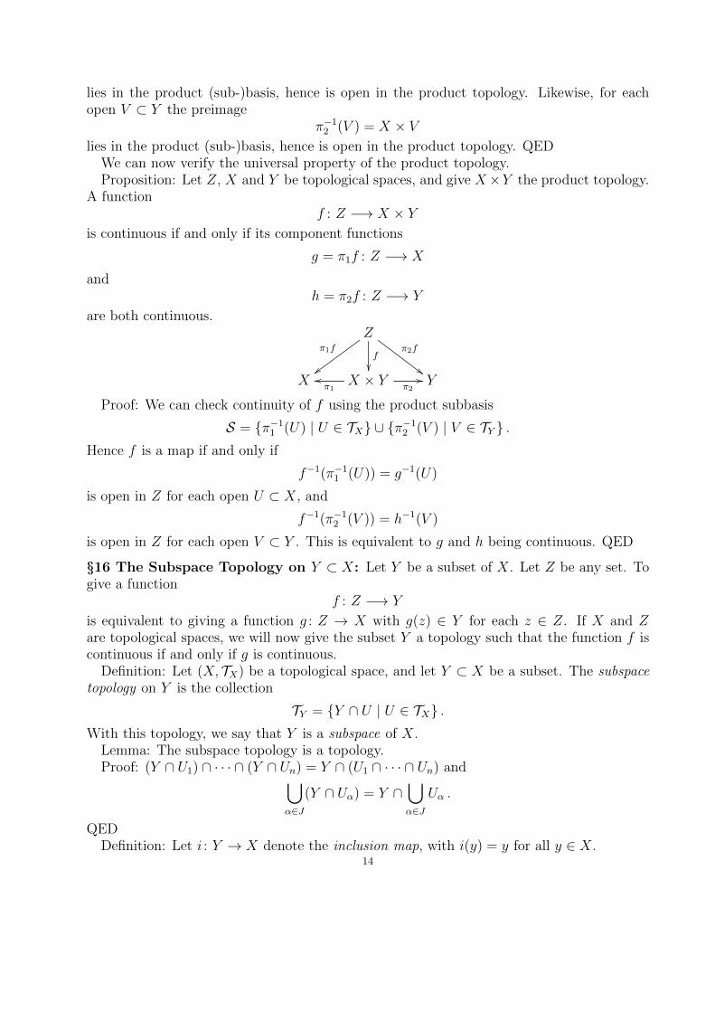
Lemma: The inclusion map is a map.Proof: i−1(U) = Y ∩ U for each U ⊂ X. QEDLemma: f : Z → Y is continuous if and only if g = if : Z → X is continuous.Proof: f−1(Y ∩ U) = (if)−1(U) for all U ⊂ X. QEDExample: Let S2 ⊂ R3 be the unit sphere, with the subspace topology. The product space

S2 × R3

consists of pairs (p, v), with p ∈ S2 and v ∈ R3. The tangent plane TpS2 to S2 at p consists

of the vectors orthogonal to p, i.e., the vectors v satisfying p · v = 0. Let the tangent bundle

TS2 = {(p, v) ∈ S2 × R3 | p · v = 0} =∐p∈S2

TpS2

be the disjoint union of all of the tangent planes, topologized as a subspace of S2×R3. Thebundle projection

π : TS2 −→ S2

is the map given by π(p, v) = p. The point preimages

π−1(p) = TpS2

are the tangent planes. A continuous vector field on S2 is a map f : S2 → TS2 such thatπf = idS2 .

TS2

π

��S2

f==

id// S2

To each point p ∈ S2 the vector field associates a tangent vector v ∈ TpS2, with f(p) = (p, v).The subspace

S2 × S2 ⊂ S2 × R3

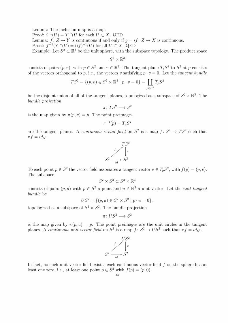
consists of pairs (p, u) with p ∈ S2 a point and u ∈ R3 a unit vector. Let the unit tangentbundle be

US2 = {(p, u) ∈ S2 × S2 | p · u = 0} ,topologized as a subspace of S2 × S2. The bundle projection

π : US2 −→ S2

is the map given by π(p, u) = p. The point preimages are the unit circles in the tangentplanes. A continuous unit vector field on S2 is a map f : S2 → US2 such that πf = idS2 .

US2

π

��S2

f<<

id// S2

In fact, no such unit vector field exists: each continuous vector field f on the sphere has atleast one zero, i.e., at least one point p ∈ S2 with f(p) = (p, 0).

15

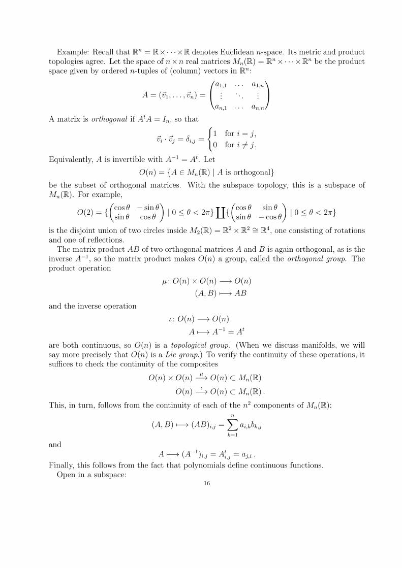
Example: Recall that Rn = R×· · ·×R denotes Euclidean n-space. Its metric and producttopologies agree. Let the space of n×n real matrices Mn(R) = Rn×· · ·×Rn be the productspace given by ordered n-tuples of (column) vectors in Rn:

A = (~v1, . . . , ~vn) =

a1,1 . . . a1,n...

. . ....

an,1 . . . an,n

A matrix is orthogonal if AtA = In, so that

~vi · ~vj = δi,j =

{1 for i = j,

0 for i 6= j.

Equivalently, A is invertible with A−1 = At. Let

O(n) = {A ∈Mn(R) | A is orthogonal}be the subset of orthogonal matrices. With the subspace topology, this is a subspace ofMn(R). For example,

O(2) = {(

cos θ − sin θsin θ cos θ

)| 0 ≤ θ < 2π}

∐{(

cos θ sin θsin θ − cos θ

)| 0 ≤ θ < 2π}

is the disjoint union of two circles inside M2(R) = R2×R2 ∼= R4, one consisting of rotationsand one of reflections.

The matrix product AB of two orthogonal matrices A and B is again orthogonal, as is theinverse A−1, so the matrix product makes O(n) a group, called the orthogonal group. Theproduct operation

µ : O(n)×O(n) −→ O(n)

(A,B) 7−→ AB

and the inverse operation

ι : O(n) −→ O(n)

A 7−→ A−1 = At

are both continuous, so O(n) is a topological group. (When we discuss manifolds, we willsay more precisely that O(n) is a Lie group.) To verify the continuity of these operations, itsuffices to check the continuity of the composites

O(n)×O(n)µ−→ O(n) ⊂Mn(R)

O(n)ι−→ O(n) ⊂Mn(R) .

This, in turn, follows from the continuity of each of the n2 components of Mn(R):

(A,B) 7−→ (AB)i,j =n∑k=1

ai,kbk,j

andA 7−→ (A−1)i,j = Ati,j = aj,i .

Finally, this follows from the fact that polynomials define continuous functions.Open in a subspace:

16

Let Y be a subspace of X. A subset V ⊂ Y is also a subset of X. If TX and TY arethe topologies on X and Y , then “V is open in X” means V ∈ TX , while “V is open in Y ”means V ∈ TY . If V is open in X, then V = Y ∩V is also open in Y , but the converse needsnot hold. The converse does hold if Y is open in X:

Lemma: Let Y be a subspace of X. If V is open in Y , and Y is open in X, then V isopen in X.

Proof: First, V = Y ∩ U for some open U in X. Second, Y is open in X. Hence theintersection Y ∩ Y = V is open in X. QED

Subspaces and bases:Lemma: Let Y ⊂ X. If B is a basis for the topology on X, then

BY = {Y ∩B | B ∈ B}is a basis for the subspace topology on Y .

Proof: We use the recognition lemma. Each Y ∩ B for B ∈ B is open in Y . For eachy ∈ Y ∩U with U open in X there is a B ∈ B with y ∈ B ⊂ U , and then y ∈ Y ∩B ⊂ Y ∩U .QED

Subspaces and products:Theorem: Let A be a subspace of X and B a subspace of Y . Then the product topology

on A×B is equal to the subspace topology from X × Y .Proof: Let U range over the open subsets of X and let V range over the open subsets of

Y , so that U ×V ranges over the product basis for X×Y . Then A∩U ranges over the opensubsets of A and B ∩ V ranges over the open subsets of B. Hence

(A ∩ U)× (B ∩ V ) = (A×B) ∩ (U ∩ V )

ranges over the product basis for A×B, as well as over a basis for the subspace topology onA×B. Hence these bases are equal, and generate the same topology. QED

§17 Closed Sets: Definition: A subset A in a topological space X is said to be closedprecisely when X − A is open.

Lemma: The closed subsets of X are the complements A = X − U of the open subsets Uin X.

Proof: X − A = U if and only if A = X − U . QEDExample: The intervals [a, b] in R are closed, because (−∞, a) ∪ (b,∞) is open.Example: Let a < b. As subsets of R, ∅ is open and closed, (a, b) is open but not closed,

[a, b] is not open but closed, and [a, b) is neither open nor closed. Hence there is no logicalimplication between the statements “A is open”, “A is not open”, “A is closed” and “A isnot closed”.

There is also, in general, no relation between the terms “a subset of a topological space isclosed” and “a collection is closed under certain operations”.

Example: The first quadrant [0,∞)× [0,∞) in R2 because its complement

(−∞, 0)× R ∪ R× (−∞, 0)

is open in R2.Example: In the trivial topology on X, the closed subsets are ∅ and X.Example: In the discrete topology on X, each subset is closed.Example: In the subspace Y = [0, 1]∪ (2, 3) of R the subsets A = [0, 1] = Y ∩ (−1/2, 3/2)

and B = (2, 3) = Y ∩ (3/2, 7/2) are both open. Since A = Y − B and B = Y − A, both17

subsets are also closed. (In Section 23 we will say that A and B form a separation of Y ,exhibiting Y as a disconnected, i.e., not connected, space.)

Theorem: Let X be a topological space. The collection C of closed subsets satisfies(a) The subsets ∅ and X are closed.(b) The union

C1 ∪ · · · ∪ Cnof any finite collection of closed subsets is closed.

(c) The intersection ⋂α∈J

Cα

of any (finite or infinite) collection of closed subsets is closed.Proof:

X − C1 ∪ · · · ∪ Cn = (X − C1) ∩ · · · ∩ (X − Cn)

is a finite intersection of open sets, hence is open.

X −⋂α∈J

Cα =⋃α∈J

(X − Cα)

is a union of open sets, hence is open. QEDLet X be any set. Given a collection C of subsets C of X satisfying (a), (b) and (c) above,

the collection T of complements U = X − C satisfies the conditions to define a topologyon X, so that C is the collection of closed subsets. Hence we could equally well define atopological space in terms of the set X and the collection C of closed subsets.

Zariski topology: Consider the complex polynomials

p(x) =d∑i=0

aixi

in one variable, where d ≥ 0 varies freely. These are the elements p(x) ∈ C[x]. The zero set

Z(p) = {z ∈ C | p(z) = 0}is a finite subset of C, unless p = 0, in which case Z(0) = C. Conversely, each finite subset

{z1, . . . , zd}of C arises as the zero set of a polynomial

p(x) = (x− z1) · · · · · (x− zd)= xd − (z1 + · · ·+ zd)x

d−1 + · · ·+ (−1)dz1 · · · zdFrancois Viete/Vieta (1540–1603). This collection C of subsets of C, i.e., the finite subsetsand the set C itself, satisfy (a), (b) and (c) of the theorem. Hence their complements

U(p) = C− Z(p) = {z ∈ C | p(z) 6= 0}and ∅ = C − C form the open sets in a topology TZar on C, called the Zariski topology.Oscar Zariski (1899–1986). This topology is coarser than the metric topology on C ∼= R2,but is finer than the discrete topology.

Cofinite topology: A similar construction works for any set X. The collection

Ccof = {F ⊂ X | F is finite} ∪ {X}18

of finite subset F ⊂ X, together with X itself, is closed under finite unions and arbitraryintersections. Hence the collection

Tcof = {X − F | F is finite} ∪ {∅}of complements of finite sets, together with ∅, define a topology on X. We call this thecofinite or finite complement topology on X.

If the set X is finite then each subset is finite, so C = Tcof = P(X) and the cofinitetopology equals the discrete topology. If X is infinite then each singleton set {x} is closed,but not open, in X, so in this case the cofinite topology is strictly coarser than the discretetopology.

Zariski topology on Cn:Consider the complex polynomials

p(x1, . . . , xn) =∑

i1,...,in≥0

ai1,...,inxi11 · · · · · xinn

in n variables, where only finitely many coefficients ai1,...,in are nonzero. These are theelements

p(x1, . . . , xn) ∈ C[x1, . . . , xn] .

The collection C of zero sets

Z(p) = {(z1, . . . , zn) | p(z1, . . . , zn) = 0}are closed under finite unions, since Z(p)∪Z(q) = Z(pq) where pq is the product of p and q.However, for n ≥ 2 it is not generally closed under intersections. Hence the collection B ofcomplements

Cn − Z(p) = {(z1, . . . , zn) | p(z1, . . . , zn) 6= 0}is not a topology. However, it is closed under finite intersections, and defines a basis for aZariski topology, with closed subsets the intersections⋂

α∈J

Z(pα) = {(z1, . . . , zn) | pα(z1, . . . , zn) = 0 for all α ∈ J}

= {(z1, . . . , zn) | p(z1, . . . , zn) = 0 for all p ∈ I}

where I = (pα | α ∈ J) ⊂ C[x1, . . . , xn] is the ideal generated by the pα. The Zariski opensets are the unions ⋃

α∈J

(Cn − Z(pα)) = Cn −⋂α∈J

Z(pα) .

In fact (David Hilbert, Emmy Noether), each Zariski open subset arises are a finite suchunion, since each ideal I in C[x1, . . . , xn] is finitely generated.

Closed sets in subspaces:Lemma: Let Y ⊂ X be a subspace. A subset A of Y is closed in the subspace topology if

and only if A = Y ∩ C for some closed C ⊂ X.Proof: The open subsets of Y are those of the form Y ∩ U for U open in X. Hence the

closed subsets of Y are those of the form

Y − Y ∩ U = Y ∩ (X − U)

for U open in X, which are those of the form Y ∩ C for C closed in X. QED19

Lemma: Let Y ⊂ X be a subspace and let A ⊂ Y . If A is closed in X then A is closed inY . The converse holds if Y is closed in X.

Proof: If A is closed in X then A = Y ∩ A is closed in Y . If A = Y ∩ C with Y and Cclosed in X then A is closed in X. QED

Interior, closure and boundary:Definition: Let X be a space and A ⊂ X any subset. The union

IntA =⋃{U | U ⊂ A, U open in X}

of the subsets of A that are open in X is an open subset of A called the interior of A in X.Lemma: IntA is the largest open subset of A, in the sense that it is open in X and

contained in A, and is maximal with this property, so that for each open U in X with U ⊂ Awe have U ⊂ IntA.

Note that IntA = A is and only if A is open in X.Example: The interior of [a, b] in R is (a, b), while the interior of [a, b] × {0} in R2 is ∅.

Hence the interior depends not only on A, but also on the containing space X.If A ⊂ C we say that A is a subset of C, or that C is a superset of A.Definition: Let X be a space and A ⊂ X any subset. The intersection

ClA =⋂{C | A ⊂ C, C closed in X}

of the supersets of A that are closed in X is a closed superset of A called the closure of Ain X.

Lemma: ClA is the smallest closed superset of A, in the sense that it is closed in X andcontains A, and is minimal with this property, so that for each closed C in X with A ⊂ Cwe have ClA ⊂ C.

Note that A = ClA is and only if A is closed in X.Lemma: X − ClA = Int(X − A) and X − IntA = Cl(X − A).Proof: U ⊂ X − A is open if and only if X − U ⊃ A is closed, and U ⊂ A is open if and

only if X − U ⊃ X − A is closed. QEDDefinition: For A ⊂ X, with X a topological space, the (topological) boundary of A in X

is

BdA = ClA− IntA .

This is a closed subset of X.Common alternative notations are A = IntA, A = ClA and ∂A = BdA. We might write

ClX A for the closure on A in X, to emphasize X.Closure in subspaces:The dependence of the closure of A on the containing space is clarified by the following

result.Theorem: Let Y ⊂ X be a subspace, and A ⊂ Y a subset. Let A denote the closure of A

in X. Then the closure of A in Y equals Y ∩ A:

ClY A = Y ∩ ClX A .

Proof: Letting {Cα}α∈J range over the closed sets in X that contain A, the intersectionsY ∩ Cα ranges over the closed sets in Y that contain A. Taking intersections we find

ClY A =⋂α∈J

(Y ∩ Cα) = Y ∩⋂α∈J

Cα = Y ∩ ClX A .

20

QEDThis suggest reserving the notation A for the closure in X, since Y ∩ A is then available

as notation for the closure in Y .Neighborhoods:Open sets express nearness (or proximity) conditions, in the sense that for x ∈ U ⊂ X

with U open in the topological space X, the condition “for all y ∈ U” is one way of saying“for all y ∈ X that are sufficiently close to x”. For example, in a metric space (X, d) thecondition “for all y ∈ B(x, ε)” is equivalent to saying “for all y ∈ X with d(x, y) < ε”.

Definition: If x ∈ U ⊂ X with U open in X, then we say that U is a neighborhood of xin X.

Replacing U by a smaller open subset V containing x, with x ∈ V ⊂ U , then expressesa more restrictive closeness condition, and “for y sufficiently close to x” usually quantifies aproperty that holds for each (arbitrarily small) neighborhood of x in X.

Some authors refer to our neighborhoods as “open neighborhood”, and call any N ⊂ Xcontaining an open neigborhood a “neighborhood”, without requiring N itself to be open:

x ∈ U ⊂ N ⊂ X .

If A∩U is nonempty, so that A∩U 6= ∅, we say that A intersects U , or that A meets U .The following theorem expresses the closure of A in terms of A meeting neighborhoods.

Theorem 17.5(a): Let A be a subset of a space X. A point x ∈ X lies in A = ClA if andonly if for each neighborhood U of x in X the intersection A ∩ U is nonempty.

In other words, x ∈ A if and only if each neighborhood of x intersects A.Proof: Let K = X − A be the complement of A. A point x ∈ X lies in IntK if and only

if there is an open U ⊂ X with x ∈ U ⊂ K. Equivalently, x ∈ IntK if and only if for someneighborhood U of x in X we have A ∩ U = ∅. Then the negated statements must also beequivalent, so that x ∈ X − IntK if and only if there exists a neighborhood U of x in Xwith A ∩ U 6= ∅. Here X − IntK = Cl(X −K) = ClA.

Theorem 17.5(b): Let B be a basis for the topology on a space X, and let A ⊂ X be asubset. A point x ∈ X lies in A = ClA if and only if for each basis element B containing xthe intersection A ∩B is nonempty.

Proof: There is an open U ⊂ X with x ∈ U ⊂ K if and only if there is a basis elementB ∈ B with x ∈ B ⊂ K. QED

Example: The closure of A = (a, b) in R is A = [a, b].Example: The closure of A = {1/n | n ∈ N} in R is A = {0} ∪ A.Example: The closure of the set A = Q of rational numbers in R is A = R. (This is

not the same as the algebraic closure, which consists of the algebraic numbers, omitting thetranscendental numbers.)

Proof: For each x ∈ R and each ε > 0 the neighborhood B(x, ε) = (x− ε, x + ε) contains(many) rational numbers.

Example: The closure of A = (−∞, 1) ∪ (1, 2) ∪ (Q ∩ (2, 4)) ∪ {5} is A = (−∞, 4] ∪ {5}.Example: If A is closed and U is open, then A−U = A∩ (X −U) is closed and U −A =

U ∩ (X − A) is open.Dense subsets:Definition: A subset A of a space X is dense in X if A = X.Lemma: A is dense in X if and only if each nonempty open ∅ 6= U ⊂ X intersects A.

21

Proof: Each x ∈ X lies in A if and only if for each x ∈ X and each open U containingx the intersection A ∩ U is nonempty. This is equivalent to asking that for each nonemptyopen U the intersection A ∩ U is nonempty.

Example: Q is dense in R.(We omit the discussion of “limit points”, less confusingly known as “cluster points”.)Convergence:Definition: Let N = {1, 2, 3, . . . } be the set of (positive) natural numbers. (Munkres writes

Z+ for this set.) A sequence in a set X is a function

N −→ X

n 7−→ xn .

We often describe the sequence by an infinite (ordered) list

x1, x2, x3, . . .

of elements in X, or write (xn)n = (xn)∞n=1 for this sequence. It is also common to write{xn}n = {xn}∞n=1, even if this suggests an unordered list, or just the set of values of thefunction n 7→ xn.

Definition: Let (X, T ) be a topological space. A sequence

x1, x2, x3, . . .

converges to a point x ∈ X if for each neighborhood U of x there is an integer N such thatxn ∈ U for all n ≥ N .

Lemma: Let B be a basis for the topology on X. A sequence (xn)n converges to x if andonly if for each basis neighborhood x ∈ B ∈ B there is an N such that xn ∈ B for all n ≥ N .

If (xn)n converges to x, then we say that x is a limit of the sequence.Example: Let (X, d) be a metric space. Then (xn)n converges to x if and only if for each

ε > 0 there is an N such that d(xn, x) < ε for each n ≥ N . Many sequences do not converge,but a sequence in a metric space can converge to at most one point.

Example: In X = {a, b} with the Sierpinski topology Ta = {∅, {a}, X}, the constantsequence xn = a for all n ≥ 1 converges to a. It also converges to b, because the onlyneighborhood of b is U = X, which contains xn for all n. A sequence in a general topologicalspace can thus converge to multiple points.

Hausdorff spaces:To ensure the uniqueness of limits, when they exist, Felix Hausdorff (1868–1942) identified

the following property.Definition: A topological space X is Hausdorff if for each pair x 6= y of distinct points in

X there are neighborhoods U and V of x and y, respectively, with U ∩ V = ∅.Lemma: Any metric space (X, d) is Hausdorff.Proof: Given x 6= y in X let ε = d(x, y)/2. Then U = B(x, ε) and V = B(y, ε) are

neighborhoods of x and y, respectively, with U ∩ V = ∅ (by the triangle inequality). QEDExample: The Sierpinski space (X, Ta) is not Hausdorff, since the only neighborhood of b

is V = X, which contains a, so no neighborhood U of a is disjoint from V .Theorem 17.10: If X is a Hausdorff space, then a sequence (xn)n in X can converge to at

most one point of X.Proof: Suppose that (xn)n converges to x and to y, with x 6= y. Choose disjoint neigh-

borhoods U and V of x and y. Then there are integers N and M so that xn ∈ U for all22

n ≥ N and xn ∈ V for all n ≥M . For n = max{M,N} this asserts that xn ∈ U ∩ V , whichis impossible, since U ∩ V = ∅. QED

Hence, in Hausdorff spaces we can speak of the limit of a sequence, granting that one suchexists.

Separation axioms:Theorem 17.8: Let X be a Hausdorff space. Then each finite subset F ⊂ X is closed.Proof: It suffices to prove that “points are closed” in Hausdorff spaces, i.e., that each

singleton set {y} ⊂ X is closed. For each point x 6= y there exist disjoint separatingneighborhoods Ux and Vx of x and y, respectively. Then

X − {y} =⋃x 6=y

Ux

is the union of the open sets Ux, hence is open. Thus {y} is closed. QEDExample: The opposite implication does not hold, since any infinite set X with the finite

complement topology is not Hausdorff. If U and V are neighborhoods of x and y, then X−Uand X − V are finite, so (X − U) ∪ (X − V ) = X − (U ∩ V ) is a union of two finite sets,hence is finite. Since X is infinite, we cannot have U ∩ V = ∅.

The Hausdorff property is one of a list of additional hypotheses one might make about atopological space, called separation axioms, or Trennungsaxiome. The condition (T1) thatpoints are closed is weaker than the Hausdorff property (T2), and stronger conditions, called(T3), (T4), regularity and normality, appear in Section 31.

§18 Continuous Functions: Recall:Definition: Let (X, TX) and (Y, TY ) be topological spaces. A function f : X → Y is

continuous if and only if for each open V in Y the preimage f−1(V ) is open in X.Note that continuity depends on the chosen topologies on X and Y , and that it suffices

to check that f−1(V ) is open in X for V ranging through a basis, or through a subbasis, forthe topology on Y .

We can reexpress continuity in terms of the closure operator A 7→ A, or in terms ofpreimages of closed sets.

Theorem 18.1: Let X and Y be topological spaces, and f : X → Y a function. Thefollowing are equivalent.

(1) The function f is continuous.

(2) For each A ⊂ X one has f(A) ⊂ f(A).(3) For each closed B ⊂ Y the preimage f−1(B) is closed in X.

Proof: If f is continuous and x ∈ A we show that f(x) ∈ f(A). Let V be a neighborhoodof f(x) in Y . Then f−1(V ) is a neighborhood of x in X, so A ∩ f−1(V ) 6= ∅. Hence

f(A) ∩ V 6= ∅, so f(x) ∈ f(A).

If f(A) ⊂ f(A) for each A, and B is closed in Y , let A = f−1(B). Then f(A) ⊂ B, so

f(A) ⊂ B, since B is closed. The hypothesis then implies f(A) ⊂ B and A ⊂ f−1(B) = A.Hence A = A is closed.

If f−1(B) is closed for each closed B, then for each open V let B = Y − V , so thatV = Y −B and

f−1(V ) = f−1(Y −B) = X − f−1(B)

is the complement of an closed in X, hence is open in X. QED23

Definition: Let x ∈ X. We say that f : X → Y is continuous at x if for each neighborhoodV of f(x) there is a neighborhood U of x with f(U) ⊂ V .

Theorem 18.1 (cont.): Let X and Y be topological spaces, and f : X → Y a function. Thefollowing are equivalent.

(1) The function f is continuous.(4) For each x ∈ X the function f is continuous at x.

Proof: If f is continuous, x ∈ X and f(x) ∈ V is open in Y , then x ∈ f−1(V ) is open inX, so U = f−1(V ) is a neighborhood of x with f(U) ⊂ V .

Conversely, if f is continuous at each x ∈ X, and V ⊂ Y is open, then for each x ∈ f−1(V )we can choose a neighborhood Ux of x with f(Ux) ⊂ V . Then Ux ⊂ f−1(V ), and

U =⋃

x∈f−1(V )

Ux

is a union of open subsets, hence is open. Moreover f−1(V ) ⊂ U ⊂ f−1(V ), so f−1(V ) = Uis open. QED

The category of topological spaces:Theorem 18.2: Let X, Y , Z and W be topological spaces, and let f : X → Y , g : Y → Z

and h : Z → W be continuous. Then the composite function

g ◦ f : X −→ Z

is continuous. Moreover, each identity function

idX : X −→ X

is continuous. These satisfy

(h ◦ g) ◦ f = h ◦ (g ◦ f) : X −→ W

f ◦ idX = f : X −→ Y

idY ◦ f = f : X −→ Y .

Proof: For each open V ⊂ Z the preimage g−1(V ) is open in Y , so the preimage

(g ◦ f)−1(V ) = {x ∈ X | g(f(x)) ∈ V }= {x ∈ X | f(x) ∈ g−1(V )}= f−1(g−1(V ))

is open in X. For each open V ⊂ X, the preimage (idX)−1(V ) = V is of course open in X.QED

Following Samuel Eilenberg (1913–1998) and Saunders MacLane (1909–2005), we say thatthe collection of topological spaces and the sets of continuous functions between them, withthe composition law and identity functions given above, form a category.

Theorem 18.2 (cont.): The unique function η : ∅ → Y is continuous. For each singletonspace {y} the unique function ε : X → {y} is continuous.

Proof: The requisite preimages are empty, or all of X, hence are open. QEDWe say that ∅ is the initial topological space, and each {y} is a terminal topological

space. More generally, each function f : X → Y from a space (X, Tdisc) with the discretetopology, or to a space (Y, Ttriv) to a space with the trivial topology, will be continuous.

24

Theorem 18.2 (cont.): For each subspace A ⊂ X, the inclusion i : A → X is continuous.Hence the restriction

f |A = f ◦ i : A −→ Y

of a continuous function f : X → Y is continuous.Proof: For each open V ⊂ X the preimage i−1(V ) = A ∩ V is open in the subspace

topology on A. QEDThe converse does not hold: If a restriction f |A is continuous for some subspace A of

X, it does not generally hold that f is continuous on all of X. For the dual setting of a“corestriction”, there is a logical equivalence.

Theorem 18.2 (cont.): For each subspace B ⊂ Y , with inclusion j : B → Y , a functionf : X → B is continuous if and only if

g = j ◦ f : X −→ Y

is continuous. We call f the corestriction of g, but this terminology is not fully standard.Proof:

f−1(B ∩ V ) = g−1(V )

for all (open) V ⊂ Y . QEDExample: A constant function g : X → Y , with g(X) = {y} a singleton set, is continuous.

This is the case B = {y} and f = ε : X → {y} of the above.It is more plausible that if X = A∪B and the restrictions f |A : A→ Y and f |B : B → Y

of a function f : X → Y are continuous, then f might be continuous. Still, some hypothesesare needed.

Theorem 18.2 (cont.): Let X =⋃α∈J Uα, where each Uα is open in X. Then f : X → Y

is continuous if and only if f |Uα : Uα → Y is continuous for each α ∈ J .Proof: Let V ⊂ Y be open.

f−1(V ) =⋃α∈J

Uα ∩ f−1(V ) =⋃α∈J

(f |Uα)−1(V ) .

If f |Uα is continuous, then (f |Uα)−1(V ) is open in Uα, hence also in X since Uα is open. Ifthis holds for each α ∈ J , then the union above, which equals f−1(V ), is also open. QED

A similar result holds if X is viewed as a finite union of closed subspaces. The case of twosubspaces implies the general finite case, by induction.

Theorem 18.3 (The pasting lemma): Let X = A∪B, where A and B are closed in X. Thenf : X → Y is continuous and and only if f |A : A→ Y and f |B : B → Y are continuous.

Proof: Let C ⊂ Y be closed. Then

f−1(C) = (f |A)−1(C) ∪ (f |B)−1(C) .

Here (f |A)−1(C) is closed in the subspace A, since f |A is continuous, and is therefore alsoclosed in X, since A is closed. Likewise (f |B)−1(C) is closed in the subspace B, since f |Bis continuous, and is therefore also closed in X, since B is closed. Hence f−1(C) is a finiteunion of closed subsets of X, and is therefore closed. QED

Example: If X = [0, 1] is written as the infinite union of closed subsets

X = {0} ∪⋃n≥1

[1

n+ 1,

1

n] ,

25

a function f : [0, 1] → R can be continuous on {0} (automatically) and on each [ 1n+1

, 1n]

without being continuous at x = 0 in [0, 1]. For example, f(0) = 1 and f(x) = 0 forx ∈ (0, 1] is such a function.

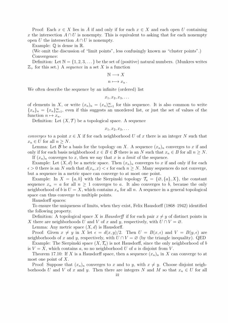
Sums of spaces: In the special case when X = A∪B with A∩B = ∅ is a disjoint union oftwo closed subspaces, or, equivalently, of two open subspaces, we say that X is the sum ofthe spaces A and B, and often write X = AtB. Let ι1 : A→ AtB and ι2 : B → AtB bethe two inclusion maps. Then f : AtB → Y is continuous if and only if fι1 = f |A : A→ Yand fι2 = f |B : B → Y are continuous.

Aι1 //

fι1 ##

A tBf

��

Bι2oo

fι2{{Y

This universal property characterizes the sum A t B of the topological spaces A and B inmanner that is dual to the characterization of the product space A×B from Section 15.

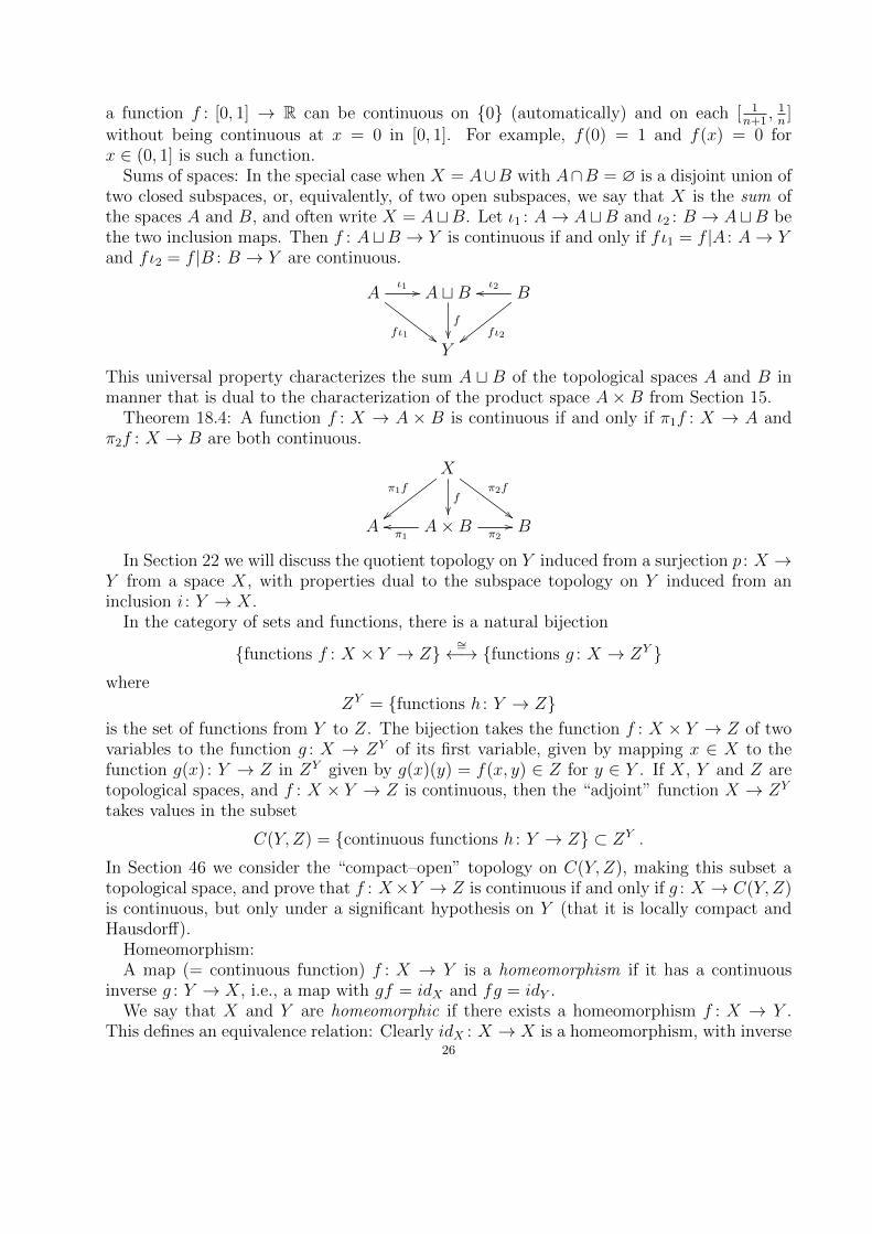
Theorem 18.4: A function f : X → A × B is continuous if and only if π1f : X → A andπ2f : X → B are both continuous.

Xπ1f

{{f��

π2f

##A A×Bπ1oo

π2// B

In Section 22 we will discuss the quotient topology on Y induced from a surjection p : X →Y from a space X, with properties dual to the subspace topology on Y induced from aninclusion i : Y → X.

In the category of sets and functions, there is a natural bijection

{functions f : X × Y → Z}∼=←→ {functions g : X → ZY }

whereZY = {functions h : Y → Z}

is the set of functions from Y to Z. The bijection takes the function f : X × Y → Z of twovariables to the function g : X → ZY of its first variable, given by mapping x ∈ X to thefunction g(x) : Y → Z in ZY given by g(x)(y) = f(x, y) ∈ Z for y ∈ Y . If X, Y and Z aretopological spaces, and f : X × Y → Z is continuous, then the “adjoint” function X → ZY

takes values in the subset

C(Y, Z) = {continuous functions h : Y → Z} ⊂ ZY .

In Section 46 we consider the “compact–open” topology on C(Y, Z), making this subset atopological space, and prove that f : X×Y → Z is continuous if and only if g : X → C(Y, Z)is continuous, but only under a significant hypothesis on Y (that it is locally compact andHausdorff).

Homeomorphism:A map (= continuous function) f : X → Y is a homeomorphism if it has a continuous

inverse g : Y → X, i.e., a map with gf = idX and fg = idY .We say that X and Y are homeomorphic if there exists a homeomorphism f : X → Y .

This defines an equivalence relation: Clearly idX : X → X is a homeomorphism, with inverse26

idX . If f : X → Y is a homeomorphism, with inverse g = f−1, then g : Y → X is ahomeomorphism with inverse f . If f : X → Y and f ′ : Y → Z are homeomorphisms, withinverses g : Y → X and g′ : Z → Y , then f ′f : X → Z is a homeomorphism with inverse gg′.This is the notion of isomorphism in the category of topological spaces and maps.

If f : (X, TX)→ (Y, TY ) is a homeomorphism, with inverse g, then the rule

TX∼=←→ TY

U 7−→ f(U) = g−1(U)

defines a bijection between the two topologies, with inverse V 7→ g(V ) = f−1(V ). Anytopological property of (X, T ), i.e., one expressed in terms of the points and open sets of Xis then logically equivalent to the corresponding property of (Y, TY ), with x replaced by f(x)and U replaced by f(U) = g−1(U).

Example: The function

f : B(0, π/2) −→ R2

r · (cos θ, sin θ) 7−→ tan r · (cos θ, sin θ)

is a homeomorphism from the open disc of radius π/2 to the full plane.Non-example: The continuous bijection

f : [0, 2π) −→ S1

x 7−→ (cosx, sinx)

is not a homeomorphism, because the inverse function

g : S1 −→ [0, 2π)

is discontinuous at (1, 0). The preimage f−1(V ) of the neighborhood V = [0, π) of g(1, 0) = 0is a half-open semicircle, from (1, 0) through (0, 1) to (−1, 0), including the endpoint (1, 0).This is not open in the subspace topology on S1, since any neighborhood of (1, 0) will containpoints (x, y) with y < 0.

Topological embeddings (= imbeddings): Given a map e : X → Y we can give the imagesubset e(X) the subspace topology from Y . There is then a surjective corestricted mapf : X → e(X). If e is injective, then f is a continuous bijection. If, moreover, f is ahomeomorphism, then we say that e : X → Y is an embedding.

Example: An embedding k : S1 → R3 is called a knot.Example: View S1 as the unit circle in R2 ∼= C. The map

e : S1 −→ S1 × S1

e(z) = (z2, z3)

defines an embedding with image a trefoil knot in the torus surface.Manifolds: Geometric topology often means the study of manifolds.Definition: Let n ≥ 0. A topological n-manifold is a locally Euclidean Hausdorff space, i.e.,

a Hausdorff space M such that each point p ∈M has a neighborhood U that is homeomorphicto (an open subset of) Rn.

If h : U ∼= h(U) with h(U) ⊂ Rn open, then V = B(h(p), ε) ⊂ h(U) for some ε > 0, andU ′ = h−1(V ) is a neighborhood of p that is homeomorphic to B(h(p), ε). Since B(h(p), ε) ∼=Rn, we might replace U with U ′ and assume that it is homeomorphic to (all of) Rn.

27

In Section 36 we add the hypothesis that a manifold admits a countable basis B ={B1, B2, B3, . . . } for its topology, and prove that each compact n-manifold can be embeddedin a Euclidean space RN for some finite N .

Manifolds often arise with more structure than a topology. In MAT4520 we study dif-ferentiable manifolds, where we also specify what it means for a function f : M → R to bedifferentiable. This means that each differentiable curve γ : [a, b]→ M has a tangent vectorγ′(t) at each point γ(t), and the tangent vectors at a point p ∈M form a tangent space TpM ,which is an n-dimensional vector space. This lets us use linear algebra and multivariablecalculus on M , where we in undergraduate courses usually had to restrict to working overan open subset of Rn. By equipping each tangent space with an inner product, we obtaina Riemannian manifold, where the length of a curve γ can be measured by integrating thelength of its tangent vectors.

‖γ‖ =

∫ b

a

|γ′(t)| dt

A 1-manifold is a curve and a 2-manifold is a surface. Each topological manifold of di-mension n ≤ 3 admits an essentially unique differentiable structure, so in this range ofdimensions the study of differentiable manifolds is the same as the study of topological man-ifolds. Each compact connected curve is homeomorphic to S1, and each compact connectedsurface can be obtained from S2 by forming a “connected sum” with finitely many tori T 2,or with finitely many projective planes RP 2. These are classified by their Euler character-istic and their (non-)orientability. William Thurston (1946–2012) formulated and partiallyproved the geometrization conjecture, saying that each compact connected 3-manifold is aconnected sum of “geometric pieces”, i.e., prime 3-manifolds that admit one of eight explicitgeometries, including the spherical, Euclidean and hyperbolic geometries. This conjecturewas proved by Grigori Perelman (1966–) in 2003, using the Ricci flow from Riemannian ge-ometry. This includes a proof of the very famous Poincare conjecture, formulated correctlyin 1904 by Henri Poincare (1854–1912), that each compact simply-connected 3-manifold ishomeomorphic to S3.

In dimension 4, there is a vast difference between topological manifolds and differen-tiable manifolds. Not every topological 4-manifold admits a differentiable structure, andother manifolds, including R4, admit an uncountable number of essentially distinct (non-diffeomorphic), differentiable structures. This follows from the work of Simon Donaldson(1957–) on “instanton gauge theory” (ask Kim Frøyshov), and Michael Freedman (1951–)on “topological surgery”. Freedman proved the 4-dimensional generalized Poincare conjec-ture in 1981 (and an book aiming to make the long proof accessible to current readers wasrecently published).

In dimensions n ≥ 5 the difference is more moderate, in that each compact connectedtopological n-manifold admits a finite number of distinct differentiable structure. The firstexamples were found in 1956 by John Milnor (1931–), who showed that S7 admits 14 other“exotic” differentiable structures than the usual one, for a total of 15, or of 28 if orientationsare taken into account. The “surgeries” used by Milnor are far easier to implement in thedifferentiable category than in the topological category, and led, in the 1960s and 1970s, to aquite good classification strategy for manifolds of dimension n ≥ 5, called “surgery theory”,mainly due to William Browder (1934–), Sergei Novikov (1938–), Dennis Sullivan (1941–)and C.T.C. Wall (1936–). A key first step was the proof in 1961 by Stephen Smale (1930–) of

28

the generalized Poincare conjecture, in all dimensions n ≥ 5. The broader theory transformsthe geometric problem into algebraic problems about quadratic forms over integral grouprings of the form Z[π], where π can be the fundamental group of a manifold.

The classification of differentiable structures on spheres was reduced by Milnor and MichelKervaire (1927–2007) to questions in homotopy theory within algebraic topology (MAT4530,MAT4540, MAT4580/9580), in areas where progress is still being made (Hill–Hopkins–Ravenel, 2016). The parametrized refinement of the surgery classification of manifolds frombeing “up to h-cobordism” to being “up to diffeomorphism” was expressed by FriedhelmWaldhausen (with Bjørn Jahren and JR) in terms of the algebraic K-theory of so-called“brave new rings”, being homotopy theoretic analogues of group rings.

—Complex manifolds.Algebraic varieties.Singularity theory.—

§19 The Product Topology: Finite products of topological spaces are defined inductively,so that

X1 × · · · ×Xn = (X1 × · · · ×Xn−1)×Xn .

Infinite products will be defined directly.Let J and X be sets. A function

x : J −→ X

α 7−→ x(α)

is an ordered J-tuple of elements in X. We call xα = x(α) the α-th coordinate of x. Let XJ

be the set of such functions/ordered J-tuples, x = (xα)α∈J .Definition: Let J be any set, and for each α ∈ J let Xα be a set. Let X =

⋃α∈J Xα. The

Cartesian product ∏α∈J

Xα

is the subset of XJ consisting of (xα)α∈J with xα ∈ Xα for each α ∈ J .In the special case when the Xα are all equal (to X),∏

α∈J

X = XJ .

For each β ∈ J , let

πβ :∏α∈J

Xα −→ Xβ

(xα)α∈J 7−→ xβ

be the projection to the β-th coordinate.Definition: Let Xα be a topological space, for each α ∈ J . Let

Sβ = {π−1β (Uβ) | Uβ open in Xβ}

29

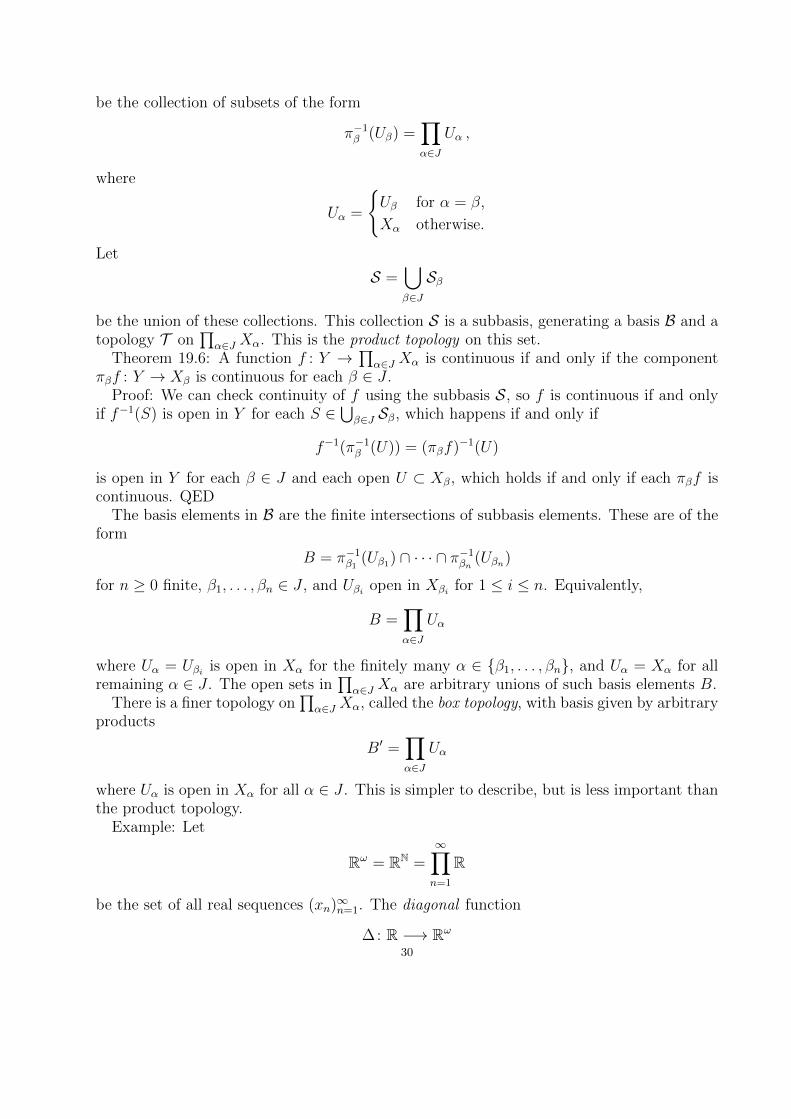
be the collection of subsets of the form

π−1β (Uβ) =

∏α∈J

Uα ,

where

Uα =

{Uβ for α = β,

Xα otherwise.

Let

S =⋃β∈J

Sβ

be the union of these collections. This collection S is a subbasis, generating a basis B and atopology T on

∏α∈J Xα. This is the product topology on this set.

Theorem 19.6: A function f : Y →∏

α∈J Xα is continuous if and only if the componentπβf : Y → Xβ is continuous for each β ∈ J .

Proof: We can check continuity of f using the subbasis S, so f is continuous if and onlyif f−1(S) is open in Y for each S ∈

⋃β∈J Sβ, which happens if and only if

f−1(π−1β (U)) = (πβf)−1(U)

is open in Y for each β ∈ J and each open U ⊂ Xβ, which holds if and only if each πβf iscontinuous. QED

The basis elements in B are the finite intersections of subbasis elements. These are of theform

B = π−1β1

(Uβ1) ∩ · · · ∩ π−1βn

(Uβn)

for n ≥ 0 finite, β1, . . . , βn ∈ J , and Uβi open in Xβi for 1 ≤ i ≤ n. Equivalently,

B =∏α∈J

Uα

where Uα = Uβi is open in Xα for the finitely many α ∈ {β1, . . . , βn}, and Uα = Xα for allremaining α ∈ J . The open sets in

∏α∈J Xα are arbitrary unions of such basis elements B.

There is a finer topology on∏

α∈J Xα, called the box topology, with basis given by arbitraryproducts

B′ =∏α∈J

Uα

where Uα is open in Xα for all α ∈ J . This is simpler to describe, but is less important thanthe product topology.

Example: Let

Rω = RN =∞∏n=1

R

be the set of all real sequences (xn)∞n=1. The diagonal function

∆: R −→ Rω

30

given by ∆(t)n = t for all t ∈ R and n ∈ N is continuous when Rω is given the producttopology, but not for the box topology, since the preimage of the box product basis element

B′ =∞∏n=1

(−1/n, 1/n)

is⋂∞n=1(−1/n, 1/n) = {0}, which is not open in R.

Theorem 19.2: Let Bα be a basis for the topology on Xα, for each α ∈ J . Then thecollection of products

B =∏α∈J

Uα

where Uα ∈ Bα for finitely many α ∈ J , and Uα = Xα for all of the remaining α, is a basisfor the product topology on

∏α∈J Xα.

Theorem 19.4: If Xα is Hausdorff for each α ∈ J , then so is∏

α∈J Xα.Theorem 19.3: Let Aα be a subspace of Xα for each α ∈ J . Then the product topology

on∏

α∈J Aα is equal to the subspace topology inherited from∏

α∈J Xα.Theorem 19.5: Let Aα be a subspace of Xα for each α ∈ J . Then∏

α∈J

Aα =∏α∈J

Aα .

Proof: (⊂) If x = (xα)α∈J lies in∏

α∈J Aα, then xα ∈ Aα for each α ∈ J . Any neighborhoodU of x in

∏α∈J Xα contains a basis neighborhood B =

∏α∈J Uα with each Uα open in Xα

(and only finitely many Uα 6= Xα). Then Uα is a neighborhood of xα ∈ Aα, for each α ∈ J ,so Aα ∩ Uα 6= ∅. Choose yα ∈ Aα ∩ Uα. Then y = (yα)α∈J lies in

∏α∈J Aα ∩

∏α∈J Uα, so B

meets∏

α∈J Aα. Hence x lies in the closure of∏

α∈J Aα.(⊃) Since Aα ⊃ Aα we have ∏

α∈J

Aα ⊃∏α∈J

Aα .

We claim that the left hand product is closed, which implies that it contains the closure ofthe right hand product. The claim follows from∏

α∈J

Aα =⋂α∈J

π−1α (Aα) ,

since Aα is closed in Xα for each α ∈ J , so that π−1α (Aα) is closed in

∏α∈J Xα by continuity

of πα, and therefore the displayed intersection of closed sets is itself closed. QEDPointwise convergence:Let J be a set and X a topological space. We can view the product topology on

XJ = {(xα)α∈J}

as giving a topology on the set of functions f : J → X. In this guise, the product topologyis also known as the pointwise convergence topology, for the following reason.

Definition: Let J be a set and X a topological space. A sequence (fn)n of functionsfn : J → X converges pointwise to a function f : J → X if for each α ∈ J the sequence(fn(α))n in X converges to f(α).

31

Proposition: Let J be a set and X a topological space. A sequence (fn)n of functionsfn : J → X converges to a function f : J → X, with respect to the product topology onXJ =

∏J X, if and only if the sequence (fn) converges pointwise to f .

(Compare Exercise 19.6 in Munkres’ book, or Proposition 2.7.5 in my course notes.)

§20 The Metric Topology: Recall the definition of a metric d on a set X. The ε-ballsBd(x, ε) form a basis for the metric topology Td on X. Such topologies are said to bemetrizable.

Example: The discrete metric

d(x, y) =

{0 if x = y,

1 if x 6= y,

induces the discrete topology, since each singleton set {x} = Bd(x, 1) is open.Consider X = Rn, with the Euclidean metric

d(x, y) = d2(x, y) =

√√√√ n∑i=1

(yi − xi)2

and the square metricρ(x, y) = d∞(x, y) = max

1≤i≤n|yi − xi| .

We haveρ(x, y) ≤ d(x, y) ≤

√nρ(x, y)

soBρ(x, ε/

√n) ⊂ Bd(x, ε) ⊂ Bρ(x, ε)

for all ε > 0.Theorem 20.3: The Euclidean topology Td, the square topology Tρ and the product topol-

ogy Tprod on Rn are all equal.Proof: Each Euclidean basis neighborhood Bd(x, ε) of x contains a square basis neighbor-

hood Bρ(x, ε/√n) of x, so Td ⊂ Tρ.

Each square basis neighborhood

Bρ(x, ε) =n∏i=1

(xi − ε, xi + ε)

is a product basis neighborhood, so Tρ ⊂ Tprod.The open intervals (a, b) form a basis for the metric topology on R, so the

B =n∏i=1

(ai, bi)

form a basis for the product topology. If x ∈ B then Bd(x, ε) ⊂ B with

ε = min1≤i≤n

{xi − ai, bi − xi} .

Hence Tprod ⊂ Td. QEDMore generally, any two norms on a finite-dimensional real vector space define the same

topology. Similar proofs show that any finite product of metric spaces is metrizable.32

Consider X = Rω. The expression

d(x, y) =

√√√√ ∞∑i=1

(yi − xi)2

does not always converge, hence does not define a metric on Rω. It does, however, define ametric on the subset

`2 = {x ∈ Rω |∞∑i=1

x2i <∞}

of square summable sequences. In fact, this is a vector subspace, and the metric comes froman inner product (and a norm) on that vector space.

Likewise, the expression

ρ(x, y) = supi∈N|yi − xi|

is not always finite, hence does not define a metric on Rω. It does, however, define a metricon the subset

`∞ = {x ∈ Rω | supi∈N|xi| <∞}

of bounded sequences. In fact, this is a vector subspace, and the metric comes from a norm(but not an inner product) on that vector space.

Bounded metric spaces:Definition: A metric space (X, d) is bounded if there is an M ∈ R such that d(x, y) ≤ M

for all x, y ∈ X.Being bounded is a property of the metric, not of the topology.Theorem 20.1: Given a metric space (X, d), let

d(x, y) = min{d(x, y), 1} .Then d defines a bounded metric on X, giving the same topology as d.

Proof: We check the triangle inequality for d. Consider x, y, z ∈ X. If d(x, y) ≥ 1 ord(y, z) ≥ 1 then

d(x, z) ≤ 1 ≤ d(x, y) + d(y, z) .

Otherwise

d(x, z) ≤ d(x, z) ≤ d(x, y) + d(y, z) .

The distances in the metric space (X, d) are bounded by M = 1. For x ∈ X and 0 < ε ≤ 1we have

Bd(x, ε) = Bd(x, ε) ,

and these form bases for the topologies Td and Td, which must therefore be equal. QEDThe supremum ρ(x, y) = supi∈N |yi−xi| would always be defined if we replaced the distance

d(a, b) = |b− a| in R with its bounded variant d. This works for arbitrary metric spaces andindex sets.

Uniform metric: Let (X, d) be any metric space, and let J be any set. For x, y ∈ XJ let

ρ(x, y) = supα∈J

d(xα, yα) ,

where d(xα, yα) = min{d(xα, yα), 1}.33

Lemma: ρ defines a metric on XJ , and the associated topology Tρ is called the uniformtopology.

Proof: The triangle inequality follows from

supα∈J

(d(xα, yα) + d(yα, zα)) ≤ supα∈J

d(xα, yα) + supα∈J

d(yα, zα) .

QEDTheorem 20.4: The uniform topology on XJ is finer than the product topology.Proof: The product topology on XJ is the coarsest topology for which all of the projections

πβ : XJ −→ X

are continuous. Hence it suffices to show that πβ is continuous when XJ is given the uniformtopology, for each β ∈ J . Fix a point x = (xα)α∈J ∈ XJ and a β ∈ J , so that πβ(x) = xβ.The metric basis neighborhoods of xβ in (X, d) are of the form Bd(xβ, ε) for ε > 0. For anyy ∈ XJ we have

d(xβ, yβ) ≤ ρ(x, y) ,

soBρ(x, ε) ⊂ π−1

β (Bd(xβ, ε)) ,

and πβ is continuous. QEDAddendum: When J is infinite, the uniform topology is strictly finer than the product

topology.The (proof of the) next theorem shows that a countable product of metric spaces, such

as R, is also metrizable. An example in the next section shows that for uncountable J , theproduct space RJ will not be metrizable.

Theorem 20.5: Let d(a, b) = min{|b − a|, 1} be the standard bounded metric on R. Forx, y ∈ Rω let

D(x, y) = supi∈N

d(xi, yi)

i.

Then D is a metric that induces the product topology on Rω.Proof: The triangle inequality for D follows from that for d and

supi

d(xi, yi) + d(yi, zi)

i≤ sup

i

d(xi, yi)

i+ sup

i

d(yi, zi)

i.

To show that the product topology is finer than the metric topology, let U be a metricneighborhood of x. Then there exists ε > 0 with x ∈ BD(x, ε) ⊂ U . We will find a productneighborhood V of x with V ⊂ BD(x, ε). To do so, choose an N ∈ N with 1/N < ε. Let

V = (x1 − ε, x1 + ε)× · · · × (xN − ε, xN + ε)× R× R× . . .be a product basis neighborhood of x = (xi)i. For any y ∈ Rω we have

D(x, y) = supi

d(xi, yi)

i≤ max{ d(x1, y1)

1, . . . ,

d(xN , yN)

N,

1

N}

sinced(xi, yi)

i≤ 1

i≤ 1

Nfor all i ≥ N . If y ∈ V then d(xi, yi)/i < ε/i ≤ ε for 1 ≤ i ≤ N , and 1/N < ε by our choiceof N , so D(x, y) < ε. Hence V ⊂ BD(x, ε).

34

Conversely, to show that the metric topology is finer than the product topology, considera product basis neighborhood

W =∏i∈N

Ui

of x, with Ui open in R for i ∈ {α1, . . . , αn} and Ui = R for the remaining i ∈ N. Thenxi ∈ (xi − εi, xi + εi) ⊂ Ui for some 0 < εi ≤ 1, for each i ∈ {α1, . . . , αn}. We will find anε > 0 with BD(x, ε) ⊂ W . To do so, choose

ε = min{εii| i = α1, . . . , αn} .

If y ∈ BD(x, ε) thend(xi, yi)

i≤ D(x, y) < ε ≤ εi

ifor each i ∈ {α1, . . . , αn}. Hence d(xi, yi) < εi ≤ 1 and |yi− xi| < εi for each of these i. Thisensures that y ∈ W , so BD(x, ε) ⊂ W . QED

§21 The Metric Topology (continued): We suppose known:Theorem 21.1: If (X, dX) and (Y, dY ) are metric spaces, then a function f : X → Y is

continuous with respect to the associated topologies if and only if for each x ∈ X and ε > 0there is a δ > 0 such that dX(x, y) < δ implies dY (f(x), f(y)) < ε.

Lemma 21.4: The functions

R× R −→ R(x, y) 7−→ x+ y

(x, y) 7−→ x− y(x, y) 7−→ x · y

and

R× (R− {0}) −→ R(x, y) 7−→ x/y

are continuous.The proof can be carried out with the ε-δ characterization of continuity. This implies:Theorem 21.5: If X is a topological space and f, g : X → R are continuous functions, then

so are f + g, f − g and f · g. If g(x) 6= 0 for all x ∈ X, then f/g is continuous.Proof: We can view g as a map to R− {0} and write f/g as the composition

X(f,g)−→ R× (R− {0}) /−→ R ,

where the function (f, g) to the product is continuous since each component function hasthis property. The other cases are similar. QED

Subspace metric:If (X, d) is a metric space and A ⊂ X any subset, then the restriction

dA = d|A× A : A× A −→ Rdefines a metric on A called the subspace metric. The metric topology on A associated todA is equal to the subspace topology.

The sequence lemma:35

In a metric space (X, d), the (countable) collection

{Bd(x, 1/n) | n ∈ N}forms a neighborhood basis at x, in the sense that each open U ⊂ X with x ∈ U contains (atleast) one of these neighborhoods Bd(x, 1/n). After all, each such open U contains Bd(x, ε)for some ε > 0, and then it also contains Bd(x, 1/n) for (all) n with 1/n < ε.

This lets us characterize the points in the closure A of a subset A ⊂ X as the limits (in X)of sequences in A. (Do not confuse these limits with the limit points = cluster points ofSection 17.)

Lemma 21.2 (The sequence lemma): Let X be a topological space, and let A ⊂ X.(a) If (an)n is a sequence of points in A, and an → x in X as n→∞, then x ∈ A.(b) If X is metrizable, then the converse holds: For each x ∈ A there is a sequence (an)n

in A with an → x in X as n→∞.Proof: (a) Convergence of (an)n to x means that for each neighborhood U of x in X there

is an N such that an ∈ U for all n ≥ N . Hence aN ∈ A ∩ U , so U meets A. This impliesthat x ∈ A.

(b) Suppose x ∈ A. Then each neighborhood Bd(x, 1/n) meets A, so we can choosean ∈ A ∩ Bd(x, 1/n). We claim that (an)n converges to x in X. To check this, consider anyneighborhood U of x. It contains Bd(x, ε) for some ε > 0, hence also contains Bd(x, 1/n) foreach 1/n < ε. Thus an ∈ Bd(x, 1/n) ⊂ U for all n ≥ N , where N is chosen so that 1/N < ε.This implies that an → x as n→∞. QED

Example: If J is uncountable, then RJ =∏

J R is not metrizable. See Munkres (page 133)for a proof that RJ does not satisfy part (b) of the sequence lemma.

Sequential characterization of continuity:For metric spaces, we can characterize continuity in terms of preservation of limits of

sequences.Theorem 21.3: Let f : X → Y be a function.(a) If f is continuous, and xn → x in X as n→∞, then f(xn)→ f(x) in Y as n→∞.(b) If X is metrizable, then the converse holds: Suppose that whenever (xn)n is a sequence

with xn → x in X as n→∞, then f(xn)→ f(x) in Y as n→∞. Then f is continuous.Proof: (a) Let V be any neighborhood of f(x). Then f−1(V ) is a neighborhood of x, so

there is an N with xn ∈ f−1(V ) for all n ≥ N . Then f(xn) ∈ V for all n ≥ N . Hencef(xn)→ f(x) in Y as n→∞.

(b) Let A ⊂ X be arbitrary. We prove that f(A) ⊂ f(A) and appeal to Theorem 18.1.Let x ∈ A. Since X is metrizable, there exists a sequence (an)n in A with an → x in Xas n → ∞. By assumption, (f(an))n then converges to f(x) in Y as n → ∞. Since this

is a sequence in f(A), it follows that f(x) ∈ f(A). Hence f(A) ⊂ f(A), and f must becontinuous. QED

Note that only the existence of the countable neighborhood basis around each point x ∈X was needed for the sequence lemma and the convergent sequence characterization ofcontinuity, not the full existence of a metric d. We return to this in Section 30.

Uniform convergence:For a set J and metric space (X, d) we can think of the product topology and the uniform

topology on ∏J

X = {(xα)α∈J}

36

as giving topologies on the function set

XJ = {f : J −→ X} .This leads to two notions of convergence on the set XJ . As noted in Section 19, thefirst of these is that of pointwise convergence, which makes sense for arbitrary topologi-cal spaces X. The second notion is known as uniform convergence, and only makes sense formetric spaces (X, d).

Definition: Let J be a set and (X, d) a metric space. A sequence (fn)n of functionsfn : J → X converges uniformly to a function f : J → X if for each ε > 0 there is aninteger N such that d(fn(α), f(α)) < ε for all n ≥ N and α ∈ J .

Proposition: Let J be a set and (X, d) a metric space. Let

ρ(f, g) = supα∈J

d(f(α), g(α))

be the associated uniform metric on XJ . A sequence (fn)n of functions fn : J → X convergesto a function f : J → X, with respect to the uniform topology on XJ , if and only if thesequence (fn) converges uniformly to f .

(See Section 21, Exercise 7 in Munkres’ book.)Uniform limit theorem:In the case where J is also a topological space, it makes sense to restrict attention to the

functions f : J → X that are continuous. Let us switch from J and X to X and Y , so thatwe are considering the subset C(X, Y ) of Y X .

Theorem 21.6 (Uniform limit theorem): Let X be a topological space and (Y, d) a metricspace. Let fn : X → Y for n ≥ 1 be a sequence of continuous functions. If (fn)n convergesuniformly to a function f : X → Y , then f is continuous.

Proof: We show that f is continuous at each point x0 ∈ X. Let V be a neighborhoodof f(x0) in Y . Choose ε > 0 so that B(f(x0), ε) ⊂ V . By uniform convergence fn → f asn→∞ we can choose N ∈ N so that for all x ∈ X we have

d(fN(x), f(x)) < ε/3 .

By continuity of fN : X → Y at x0 we can choose a neighborhood U of x0 in X with

d(fN(x0), fN(x)) < ε/3

for all x ∈ U . Then

d(f(x0), f(x)) ≤ d(f(x0), fN(x0)) + d(fN(x0), fN(x)) + d(fN(x), f(x))

< ε/3 + ε/3 + ε/3 = ε

for all x ∈ U . QED

§22 The Quotient Topology: We turn to how to paste topological spaces together. IfX = A ∪ B is a union of two subsets, and A and B have assigned topologies, we can formtheir disjoint union A tB with the sum topology, and there is a surjective function

p : A tB −→ X .

A subset U ⊂ AtB is open in the sum topology if and only if A∩U is open in A and B∩Uis open in B. We will now see how to use the surjection p to specify a topology on X, calledthe quotient topology from A tB.

37

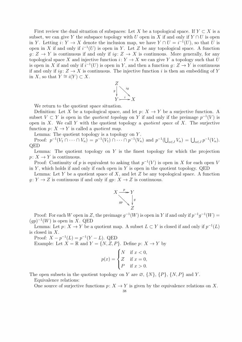
First review the dual situation of subspaces: Let X be a topological space. If Y ⊂ X is asubset, we can give Y the subspace topology with U open in X if and only if Y ∩ U is openin Y . Letting i : Y → X denote the inclusion map, we have Y ∩ U = i−1(U), so that U isopen in X if and only if i−1(U) is open in Y . Let Z be any topological space. A functiong : Z → Y is continuous if and only if ig : Z → X is continuous. More generally, for anytopological space X and injective function i : Y → X we can give Y a topology such that Uis open in X if and only if i−1(U) is open in Y , and then a function g : Z → Y is continuousif and only if ig : Z → X is continuous. The injective function i is then an embedding of Yin X, so that Y ∼= i(Y ) ⊂ X.

Z

g

��

ig

Y // i // X

We return to the quotient space situation.Definition: Let X be a topological space, and let p : X → Y be a surjective function. A

subset V ⊂ Y is open in the quotient topology on Y if and only if the preimage p−1(V ) isopen in X. We call Y with the quotient topology a quotient space of X. The surjectivefunction p : X → Y is called a quotient map.

Lemma: The quotient topology is a topology on Y .Proof: p−1(V1 ∩ · · · ∩ Vn) = p−1(V1) ∩ · · · ∩ p−1(Vn) and p−1(

⋃α∈J Vα) =

⋃α∈J p

−1(Vα).QED

Lemma: The quotient topology on Y is the finest topology for which the projectionp : X → Y is continuous.

Proof: Continuity of p is equivalent to asking that p−1(V ) is open in X for each open Vin Y , which holds if and only if each open in Y is open in the quotient topology. QED

Lemma: Let Y be a quotient space of X, and let Z be any topological space. A functiong : Y → Z is continuous if and only if gp : X → Z is continuous.

Xp // //

gp

Y

g

��Z

Proof: For eachW open in Z, the preimage g−1(W ) is open in Y if and only if p−1g−1(W ) =(gp)−1(W ) is open in X. QED

Lemma: Let p : X → Y be a quotient map. A subset L ⊂ Y is closed if and only if p−1(L)is closed in X.

Proof: X − p−1(L) = p−1(Y − L). QEDExample: Let X = R and Y = {N,Z, P}. Define p : X → Y by

p(x) =

N if x < 0,

Z if x = 0,

P if x > 0.

The open subsets in the quotient topology on Y are ∅, {N}, {P}, {N,P} and Y .Equivalence relations:One source of surjective functions p : X → Y is given by the equivalence relations on X.

38

Definition: A relation on X is a subset R ⊂ X ×X. We write xRy if (x, y) ∈ R. We saythat R is an equivalence relation if

(1) xRx for all x ∈ X;(2) If xRy then yRx;(3) If xRy and yRz then xRz.We then write [x] = {y ∈ X | xRy} for the equivalence class of x with respect to R. This

is a subset of X. Note that [x] = [y] if and only if xRy. Let

X/R = {[x] | x ∈ X}

be the collection of equivalence classes with respect to R. The canonical projection

q : X −→ X/R

x 7−→ [x]

is surjective.If X is a topological space and R an equivalence relation on X, then we can give X/R

the quotient topology from the canonical projection q : X → X/R, making X/R a quotientspace of X and making q a quotient map. Here V ⊂ X/R is open if and only if

q−1(V ) = {x ∈ X | [x] ∈ V }

is open in X.Given any surjection p : X → Y , we can define an equivalence relation R by setting xRy

for (x, y) ∈ X×X if and only if p(x) = p(y) in Y . Then p factors as the canonical projectionq : X → X/R followed by the bijection X/R ∼= Y sending [x] to p(x). If p : X → Y is aquotient map, and we give X/R the quotient topology, then X/R ∼= Y is a homeomorphism.(This is dual to the situation for embeddings.)

Example: Let X = S2 be the unit sphere in R3, and define an equivalence relation R byxRy if y = ±x. The equivalence classes [x] = {x,−x} are the (unordered) pairs of antipodalpoints. The set RP 2 = X/R equals the collection of such pairs, and is called the (real)projective plane. The canonical projection

q : S2 −→ RP 2

maps x ∈ S2 to [x] = {x,−x}. The quotient topology on RP 2 has as open subsets theV ⊂ RP 2 for which q−1(V ) is open in S2.

Can also view RP 2 as the space of lines L ⊂ R3 through the origin. For each fixed planeα ⊂ R3 through the origin, the set of L ⊂ α define a subset of RP 2 called a projective line.The projective points and lines satisfy similar axioms to those of the Euclidean plane, butthere are no parallel lines. Any two projective points lie on precisely one projective line,and any two projective lines meet in precisely one projective point. (Compare MAT4510 –Geometric Structures.)

(We could also construct RP 2 as a quotient space of R3 − {0}, with p : R3 − {0} → RP 2

identifying nonzero x, y ∈ RP 3 if Rx = Ry, i.e., if there is a nonzero λ ∈ R with y = λx.In this case, the quotient topologies from S2 and from RP 3 − {0} agree, as we may checklater.)

Open maps and closed maps:39

Definition: A continuous function f : X → Y is an open map if for each open U ⊂ X theimage f(U) is open in Y . It is a closed map if for each closed K ⊂ X the image f(K) isclosed in Y .

Lemma: Let p : X → Y be continuous and surjective. If p is an open map, or a closedmap, then p is a quotient map.

Proof: We must show that if V ⊂ Y and p−1(V ) is open in X, then V is open. Bysurjectivity, p(p−1(V )) = V , so if p−1(V ) is open in X and p is an open map, then V is openin Y .

In the closed map case, we show that if L ⊂ Y and p−1(L) is closed in X, then L isclosed in Y . The converse holds by the closed set criterion for the continuity of p, so thiswill characterize the topology on Y as being the quotient topology induced from X alongp : X → Y . By surjectivity, p(p−1(L)) = L, so if p−1(L) is closed in X and p is a closed map,then L is closed in Y . QED

Some maps are both open and closed. Some quotient maps are neither open nor closed.Example: Let π1 : R × R → R be the first projection. This is continuous and surjective.

Moreover, it is an open map, since π1(U × V ) = U is open in R for each element U × V inthe product basis for R×R. Hence it is also a quotient map. It is not a closed map, because

C = {(x, y) ∈ R× R | xy = 1}

is closed in R× R, while the image π1(C) = R− {0} is not closed in R.See Munkres’ Section 22 for more on the (lack of) compatibility between quotient topolo-

gies and other constructions, such as products and subspaces.

§23 Connected Spaces: The Intermediate Value Theorem asserts that for a continuousfunction f : [a, b] → R each r between f(a) and f(b) arises as a value r = f(c) for somec ∈ [a, b]. This is a consequence of the fact that [a, b] is connected, which is a topologicalproperty that we now discuss for general topological spaces.

We will say that a topological space X is disconnected if there is a continuous surjection (=surjective map) f : X → {a, b}, where {a, b} has the discrete topology. Letting U = f−1(a)and V = f−1(b), this is equivalent to asking that U ∪V = X, U ∩V = ∅, U and V are openin X, and U and V are nonempty.

Definition: A separation of a topological space X is a pair of nonempty open subsetsU, V ⊂ X with U ∪ V = X and U ∩ V = ∅. If a separation of X exists, then X isdisconnected. If no separation of X exists, then X is connected.

By this definition, the empty space ∅ is connected. Some authors require connected spacesto be nonempty, so that there is a three-case distinction: empty, connected or disconnected.This is similar to the classification of natural numbers as the unit, the primes and thecomposite numbers.

Lemma: A (nonempty) space X is connected if and only if the only open and closedsubsets U ⊂ X are ∅ and X.

Proof: If U and V are a separation of X, then U is open and closed, and U 6= ∅, U 6= X.The converse also holds, with V = X − U . QED

Example: X = {a, b} with the trivial topology is connected, since the only open and closedsubsets are ∅ and X.

Connected subspaces:40

Recall that for A ⊂ Y ⊂ X we write A for the closure of A in X. The following isLemma 23.1, reformulated in terms of closures in place of “limit points”.

Lemma: Let Y ⊂ X be a subspace. A separation of Y is a pair A and B of nonemptysubsets with A ∪B = Y , A ∩B = ∅ and A ∩ B = ∅.

Proof: If A and B is a separation of Y , then B is closed in Y , so that B = Y ∩ B, whichimplies

A ∩ B = A ∩ Y ∩ B = A ∩B = ∅ .

Switching the roles of A and B proves that A ∩B = ∅.Conversely, given A and B as above, A ∩B ⊂ A ∩ B = ∅, so A ∩B = ∅. Then

Y ∩ B = (A ∪B) ∩ B = (A ∩ B) ∪ (B ∩ B) = ∅ ∪B = B

is closed in B, since B is closed in X, so that A = Y −B is open in Y . Symmetrically, B isopen in Y . Hence A and B is a separation of Y .

Example: Let Y = [−1, 0) ∪ (0, 1] as a subspace of R. Then A = [−1, 0) and B = (0, 1] isa separation of Y , because A = [−1, 0] does not meet B and B = [0, 1] does not meet A.

Example: Let Y = [−1, 1], A = [−1, 0] and B = (0, 1]. Then A and B is not a separationof Y , since A meets B = [0, 1] in 0. We will see that Y is connected.

Example: The subspace of rationals Q ⊂ R is disconnected. If Y ⊂ Q contains at least twopoints, say p < q, then there is an irrational r ∈ (p, q) and A = Y ∩ (−∞, r), B = Y ∩ (r,∞)is a separation of Y . Hence the only connected subspaces of Q are the singleton sets (andthe empty set).

Example: Let Y ⊂ R2 be the subspace

Y = {(x, 0) | x ∈ R} ∪ {(x, y) | x > 0, y = 1/x} .Then A = {(x, 0) | x ∈ R} and B = {(x, y) | x > 0, y = 1/x} form a separation of Y , sinceA = A and B = B are disjoint.

New connected spaces from old:Continuous images, many unions, and all products of connected spaces are connected.Theorem 23.5: The continuous image of a connected space is connected.Proof: Let f : X → Y be a surjective map, with X connected. We show that Y is

connected. Suppose that U and V is a separation of Y . Then f−1(U) and f−1(V ) are aseparation of X. ((ETC: Elaborate?)) Since X is connected, this is impossible. Hence noseparation of Y exists, and Y is connected.

More generally, if f : X → Y is continuous, but not necessarily surjective, then core-striction g : X → f(X) is a surjective map, and the argument above shows that f(X) is aconnected subspace of Y . QED

Lemma 23.2: If C and D is a separation of X, and Y ⊂ X is a connected subspace, thenY ⊂ C or Y ⊂ D.

Proof: Let A = Y ∩ C and B = Y ∩D. These are open in Y , with union Y and emptyintersection. If they are both nonempty, they give a separation of Y . Since Y is connected,no such separation exists, which means that A or B is empty, so that Y is contained in Dor C, respectively. QED

Theorem 23.3: If X =⋃α∈J Yα and p ∈

⋂α∈J Yα, with each Yα connected, then X is

connected.Proof: Suppose that C and D is a separation of X. Then p ∈ C or p ∈ D, but not both.

Suppose the first. Each Yα is contained in C or D. Since p ∈ Yα we cannot have Yα ⊂ D, so41

Yα ⊂ C. This holds for each α, so X ⊂ C. This implies C = X and D = ∅, which is not avalid separation. QED

Theorem 23.6+: Any product of connected spaces is connected.Proof: An empty product is a single point, which is connected.We prove that a product X ×Y of two connected spaces is (empty or) connected. Choose

p = (a, b) ∈ X × Y . For each x ∈ X the union

Tx = X × {b} ∪ {x} × Y

is a union of two connected spaces that meet in (x, b), hence is connected. Moreover

X × Y =⋃x∈X

Tx

is a union of connected spaces that all contain (a, b). Hence this is also connected.The case of finite products follows by induction.The case of infinite products is left to Example 23.7 and Exercise 23.10. QEDTheorem 23.4: Let Y ⊂ X be a connected subspace. If Y ⊂ Z ⊂ Y then Z is also

connected.Proof: Suppose that C and D are a separation of Z. Then the connected subspace Y lies

in C or D. Suppose the first, so that Y ⊂ C. Recall that C ∩ D = ∅. Then Z ⊂ Y ⊂ Cdoes not meet D, which contradicts the assumption that D ⊂ Z is nonempty. QED

§24 Connected Subspaces of the Real Line: Munkres considers quite general orderedsets, with the order topology from Section 14, which we have omitted. We specialize to thecase of R, with the usual metric topology.

[Follow §3.2-§3.7 from topology.pdf.]

Matrix groups. Let n ≥ 1. An n× n matrix

A = (ai,j)ni,j=1

with real entries can be viewed as an n-tuple of column vectors

A = [v1| . . . |vn]

with each vj ∈ Rn, for 1 ≤ j ≤ n. Let

Mn(R) = {A | A is a real n× n matrix}

be the vector space of all such matrices. Then there are linear isomorphisms

Mn(R) ∼= (Rn)n ∼= Rn2

.

We topologize Mn(R) so that these are homeomorphisms, where Rn2has the product topol-

ogy, which equals the metric topology from any norm on this vector space.The product of matrices defines a continuous function

· : Mn(R)×Mn(R) −→Mn(R) ,

since each entry in A ·B = AB is a polynomial in the entries of A and B.The determinant of a matrix defines a continuous function

det : Mn(R) −→ R ,42

since det(A) is a polynomial in the entries of A. Let

GLn(R) = {A ∈Mn(R) | det(A) 6= 0}be the subspace of invertible matrices, let

GL+n (R) = {A ∈Mn(R) | det(A) > 0}

be the subspace of orientation-preserving matrices, and let

SLn(R) = {A ∈Mn(R) | det(A) = 1}be the subspace of volume-preserving matrices. Each of these is preserved under matrixmultiplication, and matrix inverse, hence defines a group. In each case the multiplicationpairing, as well as the inverse map sending A to A−1, is continuous, so these are topologicalgroups.

Note that GLn(R) and GL+n (R) are open subsets of Mn(R) ∼= Rn2

hence are n2-dimensionalmanifolds. One can prove that SLn(R) is an (n2 − 1)-dimensional manifold.

Note that GLn(R) is not connected, since it maps onto R−{0}. We claim that GL+n (R) and

SLn(R) are path connected, so that GLn(R) has precisely two (path) connected components.To prove the first claim, we use Gaussian elimination/row reduction of matrices. For i 6= jlet

Ei,j(r) =

1 0 . . . 0 . . . 0 . . . 00 1 . . . 0 . . . 0 . . . 0. . . . . . . . . . . . . . . . . . . . . . . .0 0 . . . 1 . . . r . . . 0. . . . . . . . . . . . . . . . . . . . . . . .0 0 . . . 0 . . . 1 . . . 0. . . . . . . . . . . . . . . . . . . . . . . .0 0 . . . 0 . . . 0 . . . 1

be the elementary matrix that differs from the identity matrix In by an entry r in the (i, j)-thposition. The rule A 7→ Ei,j(R)A is the row operation that adds r times the j-th row to thei-th row. For any invertible matrix A there is a finite sequence of row operations that bringsA to the form

D =

λ1 0 . . . 0 . . . 0 . . . 00 λ2 . . . 0 . . . 0 . . . 0. . . . . . . . . . . . . . . . . . . . . . . .0 0 . . . λi . . . 0 . . . 0. . . . . . . . . . . . . . . . . . . . . . . .0 0 . . . 0 . . . λj . . . 0. . . . . . . . . . . . . . . . . . . . . . . .0 0 . . . 0 . . . 0 . . . λn

with λ1, . . . , λn−1 > 0. If det(A) > 0 then also λn > 0. This uses that the operation ofinterchanging two rows and changing the sign of one of them can be realized by three rowoperations of the kind mentioned above. Hence

D = Eik,jk(rk) · · · · · Ei1,j1(r1)A

for some finite k. Note that Ei,j(r)−1 = Ei,j(−r). Hence

A = Ei1,j1(−r1) · · · · · Eik,jk(−rk)D .43

Letting t ∈ [0, 1] we obtain a path

f(t) = Ei1,j1(−tr1) · · · · · Eik,jk(−trk)Din GLn(R) from f(0) = D to f(1) = A. If λ1, . . . , λn > 0 then there is also a path

g(t) = (1− t)D + tIn

from g(0) = D to g(1) = In. Hence each A ∈ GL+n (R) lies in the same path component as

In, so GL+n (R) is path connected. The surjective map

GL+n (R) −→ SLn(R)

sending A to A/ det(A)1/n shows that SLn(R) is also path connected.The subspaces GLn(R) and GL+

n (R) of Mn(R) are not closed, since the zero matrix liesin the closure of either one, hence these groups are not compact. They are, however, locallycompact. Trivially, SL1(R) = {1} is compact, but SLn(R) is not compact for n ≥ 2. Onceone proves that SLn(R) is a manifold, it follows that it is locally compact.

LetOn = {A ∈Mn(R) | AtA = In}

be the subspace of orthogonal matrices. It is a subspace of GLn(R), since det(A) = {±1}for each orthogonal A. It is preserved under the group operations, hence is a topologicalsubgroup of GLn(R). Let

SOn = {A ∈ On | det(A) = 1}be the special orthogonal group. It is a topological subgroup of SLn(R).

We claim that On and SOn are compact. To see this, note that the function

f : Mn(R) −→Mn(R)

sending A to AtA is continuous, so On = f−1(In) is the preimage of a closed point, hence isclosed in Mn(R),. In particular, for

A = [v1| . . . |vn]

orthogonal each vi is a unit vector, so

On ⊂ Sn−1 × · · · × Sn−1

is a bounded subspace of (Rn)n. Hence On is compact, and so is its closed subspace SOn =det−1(1). In fact, On is a maximal compact subgroup of GLn(R), while SOn is a maximalcompact subgroup of GL+

n (R) and of SLn(R).One can show that On and SOn are n(n−1)/2-dimensional manifolds, and are in particular

locally path connected. The Gram–Schmidt orthogonalization process defines a surjectivemap

g : GLn(R) −→ On

that maps GL+n (R) onto SOn. Hence SOn is (path) connected, and On has precisely two

(path) components.For n = 2, the group SO2 consists of the rotations(

cos θ − sin θsin θ cos θ

)for 0 ≤ θ < 2π, and is homeomorphic to S1. The other component of O2 consists of thereflections in lines through the origin, hence is also homeomorphic to RP 1 ∼= S1.

44

One often calls SOn the n-dimensional rotation group, but note that for n ≥ 4, more thanone planar rotation is usually involved. For example,

A =

cosα − sinα 0 0sinα cosα 0 0

0 0 cos β − sin β0 0 sin β cos β

∈ SO4

acts on R4 the composite of a rotation by α in the first two coordinates and a rotation by βin the last two coordinates.

45