Machine Learning Srihari

Backpropagation

Sargur Srihari

1

Machine Learning Srihari

Topics in Backpropagation•  Terminology of backpropagation1.  Evaluation of Error function derivatives2.  Error Backpropagation algorithm3.  A simple example4.  The Jacobian matrix

2

Machine Learning Srihari

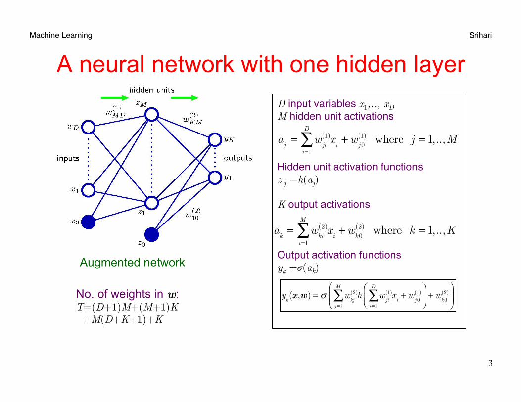
D input variables x1,.., xD M hidden unit activations

Hidden unit activation functionsz j =h(aj) K output activations Output activation functions yk =σ(ak)

A neural network with one hidden layer

3

y

k(x,w) = σ w

kj(2)

j=1

M

∑ h wji(1)

i=1

D

∑ xi+w

j 0(1)⎛

⎝⎜⎞

⎠⎟+w

k0(2)

⎛

⎝⎜

⎞

⎠⎟

a

j= w

ji(1)x

i+w

j 0(1)

i=1

D

∑ where j = 1,..,M

a

k= w

ki(2)x

i+w

k0(2)

i=1

M

∑ where k = 1,..,K

No. of weights in w: T=(D+1)M+(M+1)K =M(D+K+1)+K

Augmented network

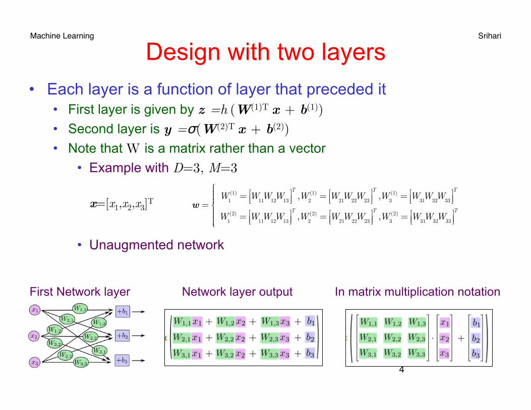
Machine Learning Srihari Design with two layers

•  Each layer is a function of layer that preceded it •  First layer is given by z =h (W(1)T x + b(1)) •  Second layer is y =σ(W(2)T x + b(2)) •  Note that W is a matrix rather than a vector

•  Example with D=3, M=3

•  Unaugmented network

4

Network layer output In matrix multiplication notation First Network layer

x=[x1,x2,x3]T

w =W

1(1) = W

11W

12W

13⎡⎣⎢

⎤⎦⎥T,W

2(1) = W

21W

22W

23⎡⎣⎢

⎤⎦⎥T,W

3(1) = W

31W

32W

33⎡⎣⎢

⎤⎦⎥T

W1(2) = W

11W

12W

13⎡⎣⎢

⎤⎦⎥T,W

2(2) = W

21W

22W

23⎡⎣⎢

⎤⎦⎥T,W

3(2) = W

31W

32W

33⎡⎣⎢

⎤⎦⎥T

⎧

⎨

⎪⎪⎪⎪

⎩⎪⎪⎪⎪

Machine Learning Srihari

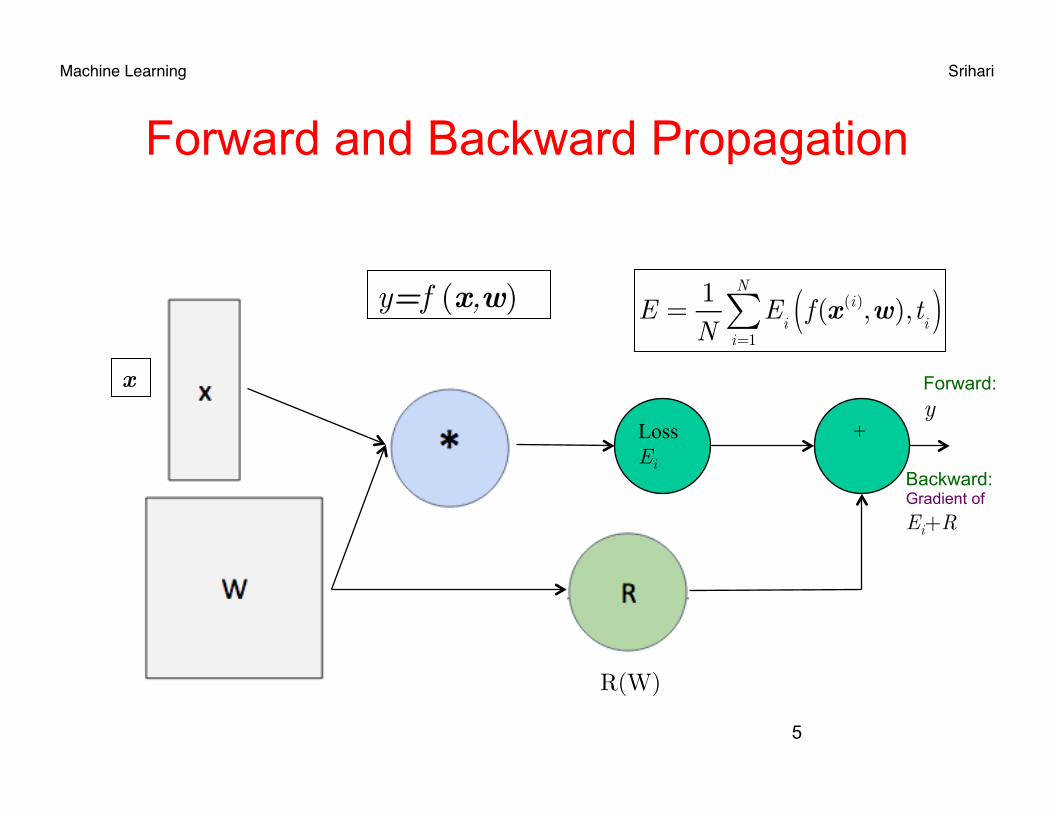
Forward and Backward Propagation

5

y=f (x,w)

Loss Ei

+

Backward: Gradient of Ei+R

R(W)

E =

1N

Ei

i=1

N

∑ f (x (i),w),ti( )

x Forward: y

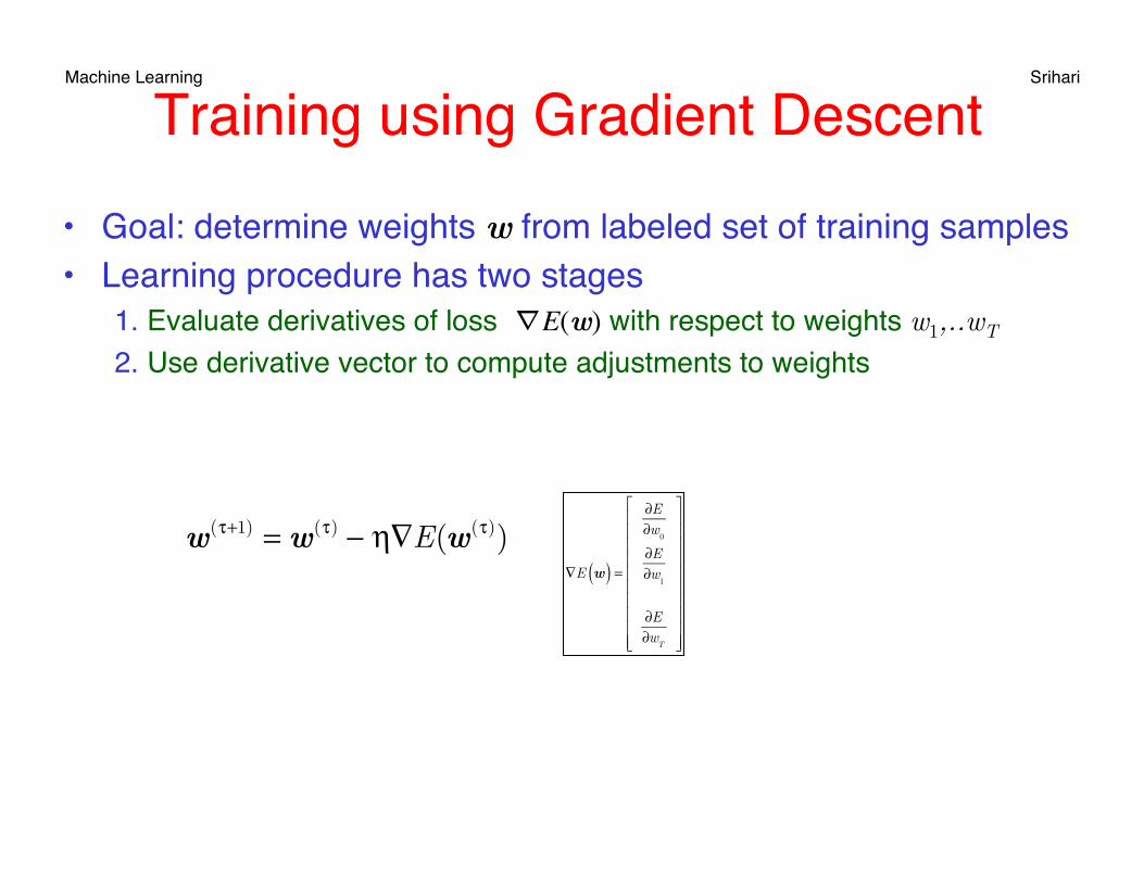
Machine Learning Srihari Training using Gradient Descent

•  Goal: determine weights w from labeled set of training samples•  Learning procedure has two stages

1. Evaluate derivatives of loss ∇E(w) with respect to weights w1,..wT 2. Use derivative vector to compute adjustments to weights

w(τ+1) = w(τ) − η∇E(w(τ))

∇E w( ) =

∂E∂w

0

∂E∂w

1

∂E∂w

T

⎡

⎣

⎢⎢⎢⎢⎢⎢⎢⎢⎢⎢

⎤

⎦

⎥⎥⎥⎥⎥⎥⎥⎥⎥⎥

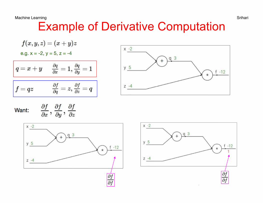
Machine Learning Srihari Example of Derivative Computation

7

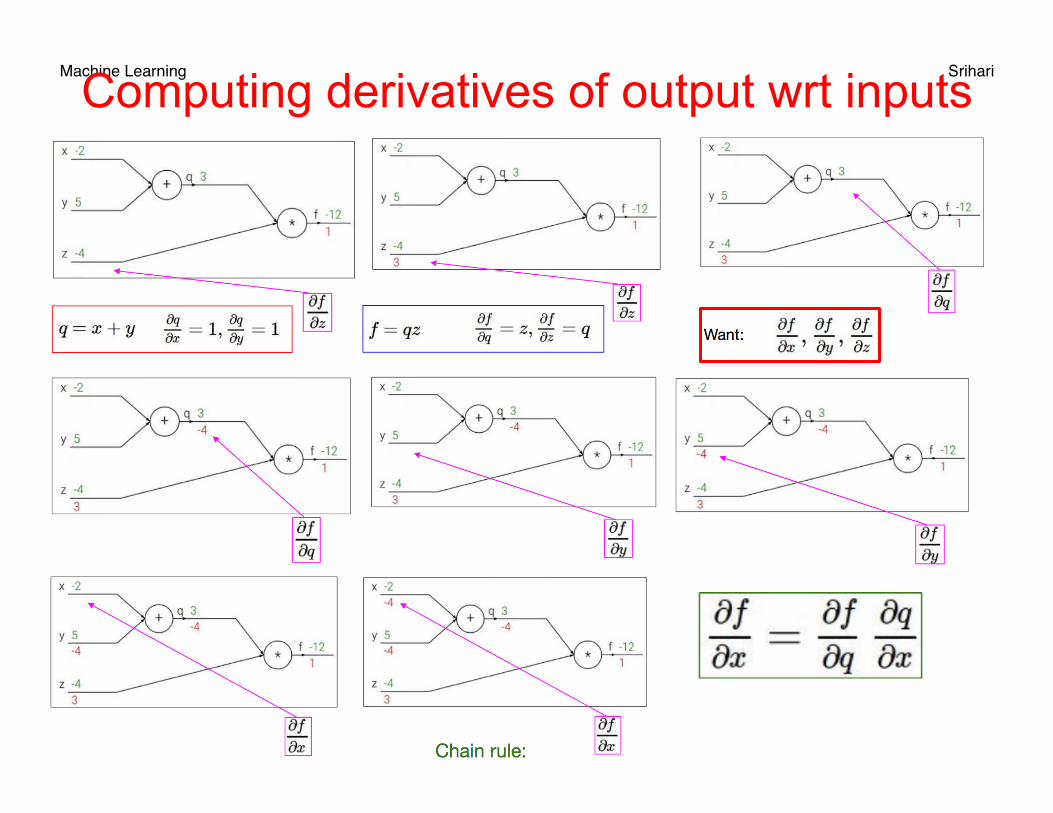
Machine Learning Srihari Computing derivatives of output wrt inputs

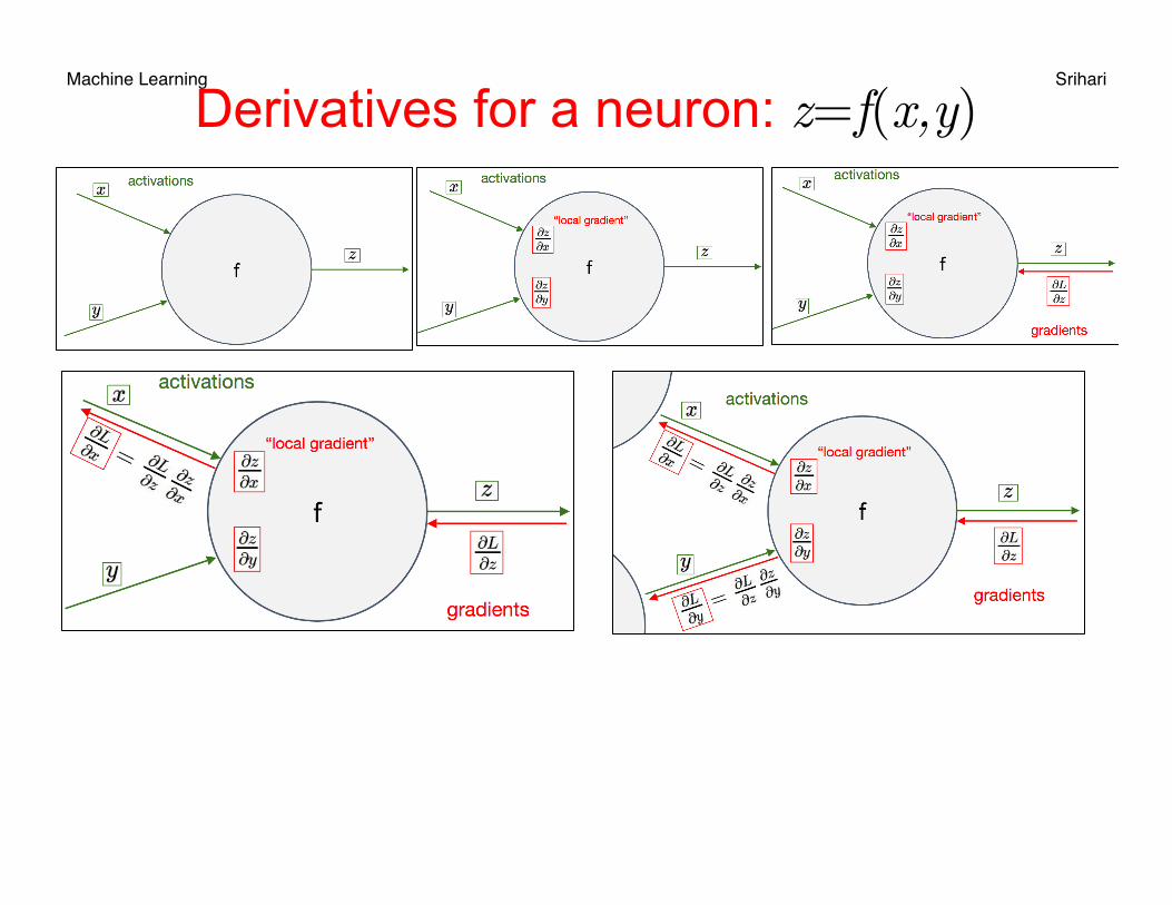
Machine Learning Srihari Derivatives for a neuron: z=f(x,y)

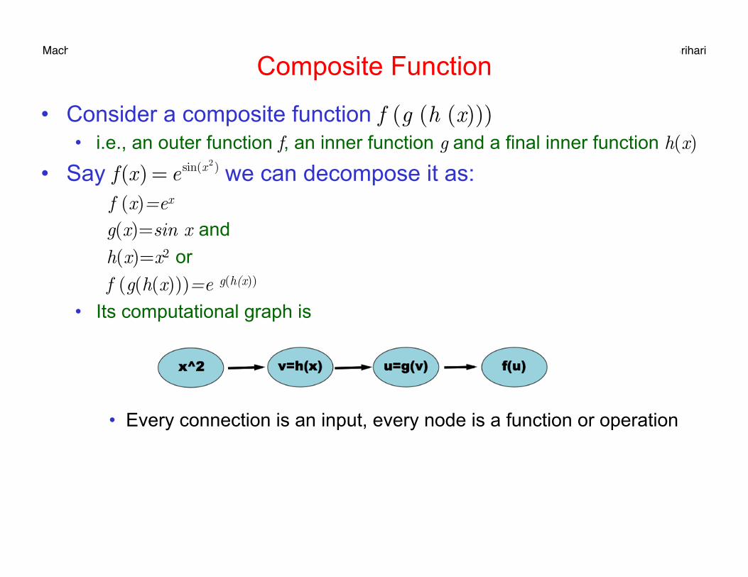
Machine Learning Srihari Composite Function

•  Consider a composite function f (g (h (x))) •  i.e., an outer function f, an inner function g and a final inner function h(x)

•  Say we can decompose it as: f (x)=ex

g(x)=sin x and h(x)=x2 or f (g(h(x)))=e g(h(x)) •  Its computational graph is

•  Every connection is an input, every node is a function or operation

f (x) = e sin(x2)

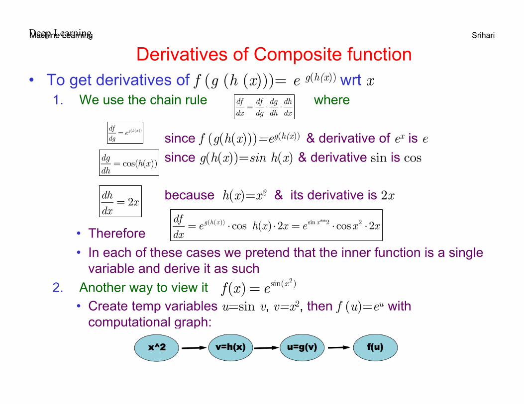
Machine Learning Srihari Derivatives of Composite function

•  To get derivatives of f (g (h (x)))= e g(h(x)) wrt x 1.  We use the chain rule where

since f (g(h(x)))=eg(h(x)) & derivative of ex is e since g(h(x))=sin h(x) & derivative sin is cos because h(x)=x2 & its derivative is 2x

•  Therefore •  In each of these cases we pretend that the inner function is a single

variable and derive it as such 2.  Another way to view it

•  Create temp variables u=sin v, v=x2, then f (u)=eu with computational graph:

dfdx

=dfdg⋅dgdh⋅dhdx

dfdg

= eg(h(x ))

dgdh

= cos(h(x))

dhdx

= 2x

dfdx

= eg(h(x )) ⋅cos h(x) ⋅2x = e sinx**2 ⋅cosx 2 ⋅2x

Deep Learning

f (x) = e sin(x2)

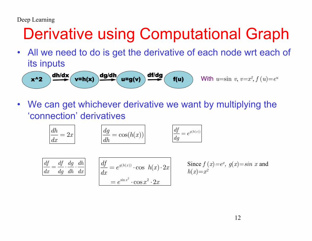
Machine Learning Srihari

Derivative using Computational Graph •  All we need to do is get the derivative of each node wrt each of

its inputs

•  We can get whichever derivative we want by multiplying the ‘connection’ derivatives

12

dfdg

= eg(h(x ))

dgdh

= cos(h(x))

dhdx

= 2x

With u=sin v, v=x2, f (u)=eu

dfdx

=dfdg⋅dgdh⋅dhdx

dfdx

= eg(h(x )) ⋅cos h(x) ⋅2x

= e sinx2

⋅cosx 2 ⋅2x

Since f (x)=ex, g(x)=sin x and h(x)=x2

Deep Learning

Machine Learning Srihari

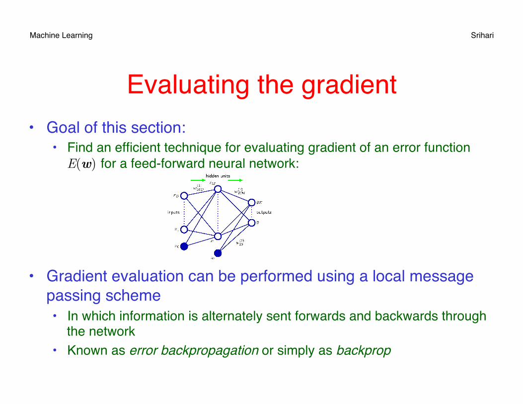
Evaluating the gradient•  Goal of this section:

•  Find an efficient technique for evaluating gradient of an error function E(w) for a feed-forward neural network:

•  Gradient evaluation can be performed using a local message passing scheme•  In which information is alternately sent forwards and backwards through

the network•  Known as error backpropagation or simply as backprop

Machine Learning Srihari

Back-propagation Terminology and Usage•  Backpropagation is term used in neural computing literature to

mean a variety of different things•  Term is used here for computing derivative of the error function wrt the

weights•  In a second separate stage the derivatives are used to compute the

adjustments to be made to the weights•  Can be applied to error function other than sum of squared

errors•  Used to evaluate other matrices such as Jacobian and Hessian

matrices•  Second stage of weight adjustment using calculated derivatives

can be tackled using variety of optimization schemes substantially more powerful than gradient descent

Machine Learning Srihari

Overview of Backprop algorithm•  Choose random weights for the network •  Feed in an example and obtain a result •  Calculate the error for each node (starting from the last stage

and propagating the error backwards) •  Update the weights •  Repeat with other examples until the network converges on the

target output

•  How to divide up the errors needs a little calculus

15

Machine Learning Srihari Evaluation of Error Function Derivatives

•  Derivation of back-propagation algorithm for•  Arbitrary feed-forward topology•  Arbitrary differentiable nonlinear activation function•  Broad class of error functions

•  Error functions of practical interest are sums of errors associated with each training data point

•  We consider problem of evaluating•  For the nth term in the error function•  Derivatives are wrt the weights w1,..wT

•  This can be used directly for sequential optimization or accumulated over training set (for batch)

16

E(w) = E

nn=1

N

∑ (w)

∇En(w)

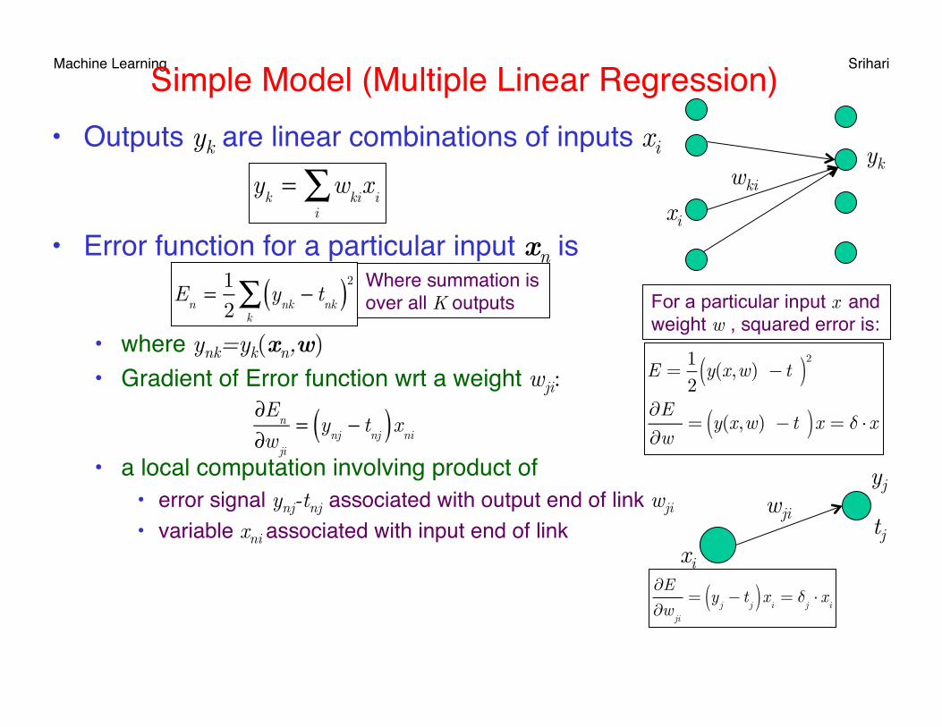
Machine Learning Srihari Simple Model (Multiple Linear Regression)•  Outputs yk are linear combinations of inputs xi

•  Error function for a particular input xn is

•  where ynk=yk(xn,w) •  Gradient of Error function wrt a weight wji:

•  a local computation involving product of•  error signal ynj-tnj associated with output end of link wji

•  variable xni associated with input end of link

E

n= 1

2y

nk− t

nk( )k∑ 2

y

k= w

kii∑ x

i

∂En

∂wji

= ynj− t

nj( )xni

xi

wji

yj

For a particular input x and weight w , squared error is:

∂E∂w

ji

= yj− t

j( )xi = δj ⋅xi

xi

wki

yk

E =12

y(x,w) − t( )2

∂E∂w

= y(x,w) − t( )x = δ ⋅x

tj

Where summation is over all K outputs

Machine Learning Srihari

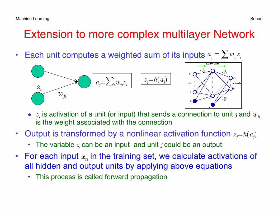
Extension to more complex multilayer Network•  Each unit computes a weighted sum of its inputs

•  zi is activation of a unit (or input) that sends a connection to unit j and wji

is the weight associated with the connection•  Output is transformed by a nonlinear activation function zj=h(aj)

•  The variable zi can be an input and unit j could be an output

•  For each input xn in the training set, we calculate activations of all hidden and output units by applying above equations

•  This process is called forward propagation

a

j= w

jii∑ z

i

aj=∑iwjizi zi wji

zj=h(aj)

Machine Learning Srihari

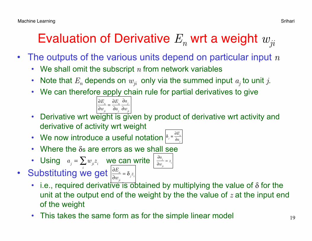
Evaluation of Derivative En wrt a weight wji

•  The outputs of the various units depend on particular input n •  We shall omit the subscript n from network variables •  Note that En depends on wji only via the summed input aj to unit j. •  We can therefore apply chain rule for partial derivatives to give

•  Derivative wrt weight is given by product of derivative wrt activity and

derivative of activity wrt weight •  We now introduce a useful notation •  Where the δs are errors as we shall see •  Using we can write

•  Substituting we get •  i.e., required derivative is obtained by multiplying the value of δ for the

unit at the output end of the weight by the the value of z at the input end of the weight

•  This takes the same form as for the simple linear model 19

∂En

∂wji

=∂E

n

∂aj

∂aj

∂wji

δ

j≡∂E

n

∂aj

∂En

∂wji

= δjz

i

a

j= w

jii∑ z

i ∂a

j

∂wji

= zi

Machine Learning Srihari

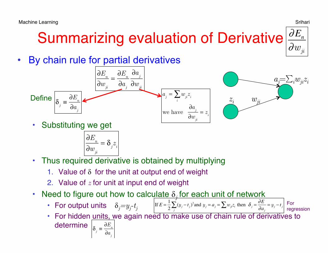
Summarizing evaluation of Derivative •  By chain rule for partial derivatives

•  Substituting we get

•  Thus required derivative is obtained by multiplying1.  Value of δ for the unit at output end of weight 2.  Value of z for unit at input end of weight

•  Need to figure out how to calculate δj for each unit of network •  For output units δj=yj-tj •  For hidden units, we again need to make use of chain rule of derivatives to

determine

zi wji

∂En

∂wji

=∂E

n

∂aj

∂aj

∂wji

δ

j≡∂E

n

∂aj

aj= w

jii∑ z

i

we have ∂a

j

∂wji

= zi

∂En

∂wji

= δjz

i

aj=∑iwjizi

Define

∂En

∂wji

δ

j≡∂E

n

∂aj

If E = 1

2(y j − t j )

2

j∑ and y j = aj = w jizi∑ then δ j =

∂E∂aj

= y j − t j Forregression

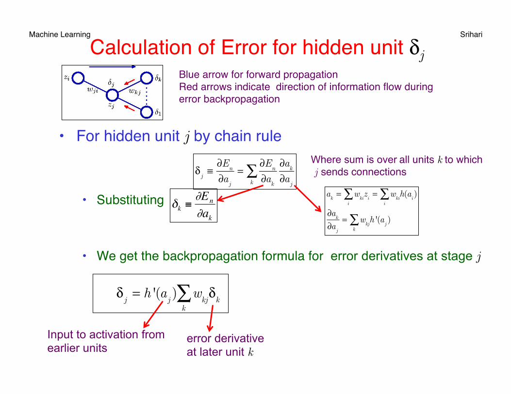
Machine Learning Srihari Calculation of Error for hidden unit δj

•  For hidden unit j by chain rule

•  Substituting

•  We get the backpropagation formula for error derivatives at stage j

Blue arrow for forward propagationRed arrows indicate direction of information flow during error backpropagation

δ

j≡∂E

n

∂aj

=∂E

n

∂akk

∑ ∂ak

∂aj

€

δk ≡∂En

∂ak

ak= w

kii∑ z

i= w

kii∑ h(a

i)

∂ak

∂aj

= wkj

k∑ h '(a

j)

δ

j= h '(a

j) w

kjk∑ δ

k

error derivative at later unit k

Where sum is over all units k to which j sends connections

Input to activation from earlier units

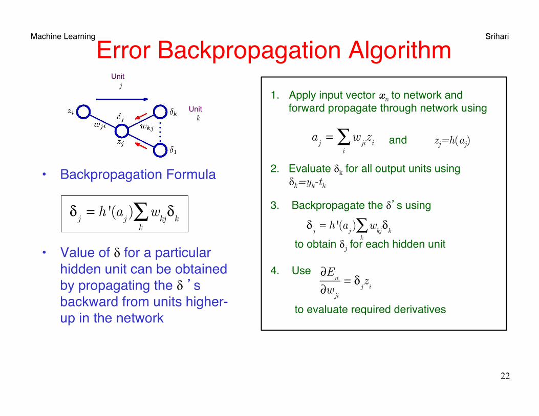
Machine Learning Srihari

3. Backpropagate the δ’s using

to obtain δj for each hidden unit

4. Use

to evaluate required derivatives

Error Backpropagation Algorithm

•  Backpropagation Formula

•  Value of δ for a particular hidden unit can be obtained by propagating the δ ’s backward from units higher-up in the network

22

δ

j= h '(a

j) w

kjk∑ δ

k

1.  Apply input vector xn to network and forward propagate through network using

a

j= w

jii∑ z

i and zj=h(aj)

2. Evaluate δk for all output units using δk=yk-tk

δ

j= h '(a

j) w

kjk∑ δ

k

∂En

∂wji

= δjz

i

Unit j

Unit k

Machine Learning Srihari

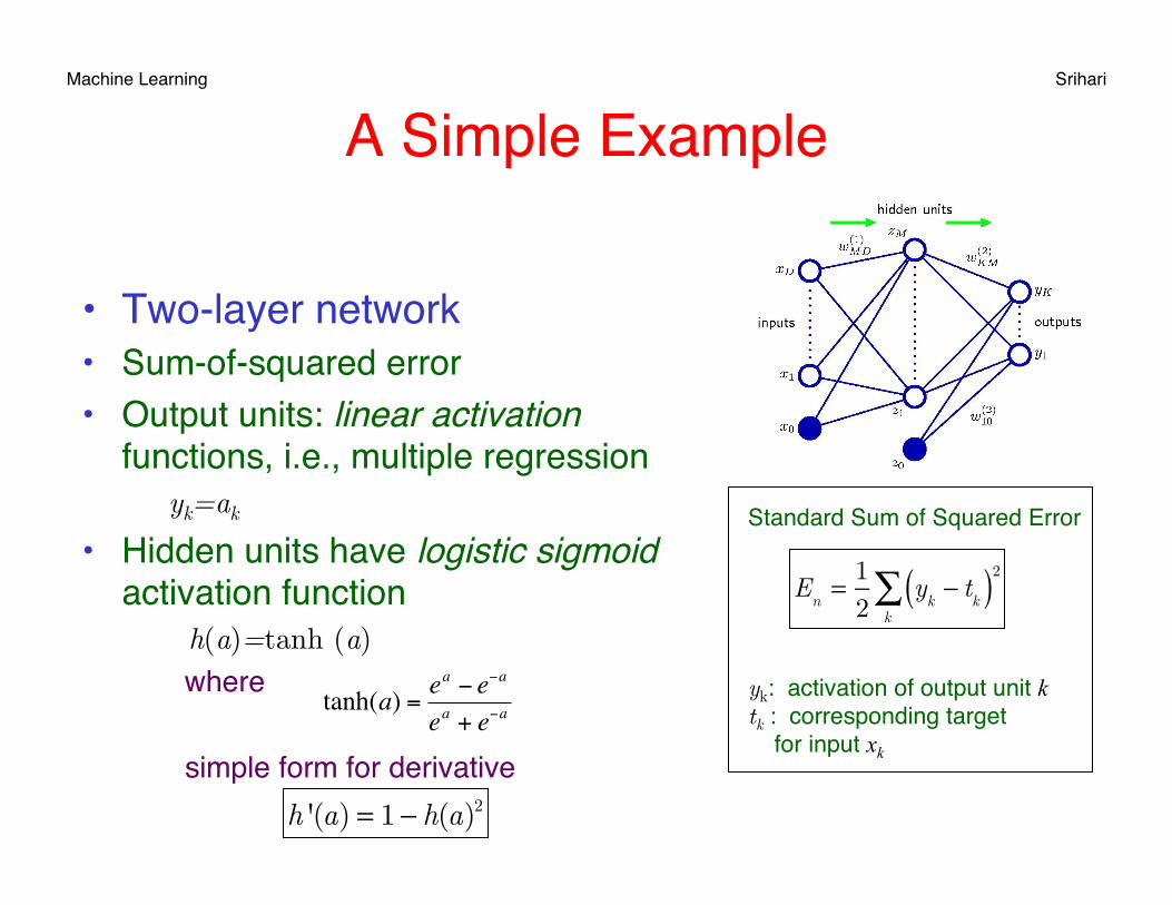
A Simple Example

•  Two-layer network•  Sum-of-squared error•  Output units: linear activation

functions, i.e., multiple regression yk=ak

•  Hidden units have logistic sigmoid activation function

h(a)=tanh (a) where

simple form for derivative

€

tanh(a) =ea − e−a

ea + e−a

h '(a) = 1 − h(a)2

Standard Sum of Squared Error

yk: activation of output unit k tk : corresponding target for input xk

E

n= 1

2y

k− t

k( )k∑ 2

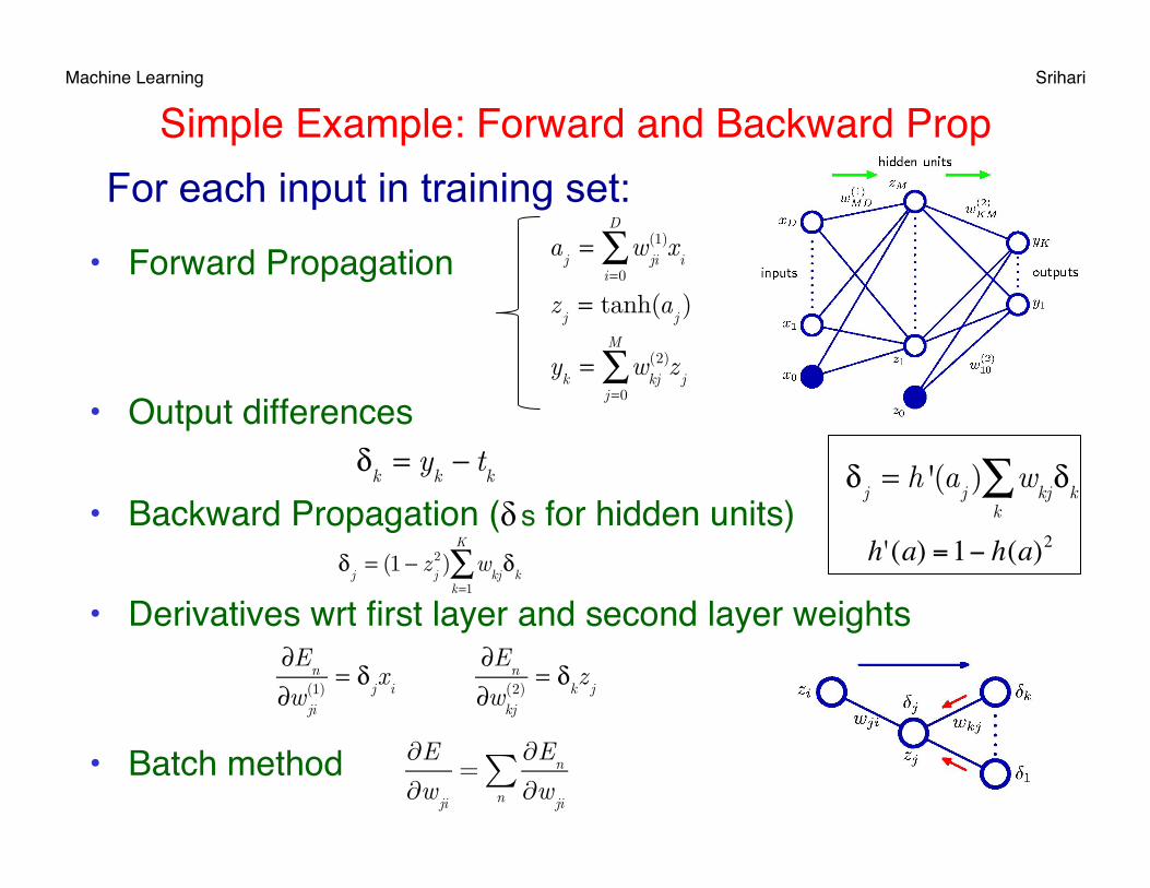
Machine Learning Srihari Simple Example: Forward and Backward Prop

•  Forward Propagation

•  Output differences

•  Backward Propagation (δ s for hidden units)

•  Derivatives wrt first layer and second layer weights

•  Batch method

aj= w

ji(1)

i=0

D

∑ xi

zj= tanh(a

j)

yk= w

kj(2)

j=0

M

∑ zj

δk= y

k− t

k

δ

j= (1 − z

j2) w

kjδ

kk=1

K

∑

∂En

∂wji(1)

= δjx

i

∂En

∂wkj(2)

= δkz

j

For each input in training set:

€

h'(a) =1− h(a)2 δ

j= h '(a

j) w

kjk∑ δ

k

∂E

∂wji

=∂E

n

∂wjin

∑

Machine Learning Srihari

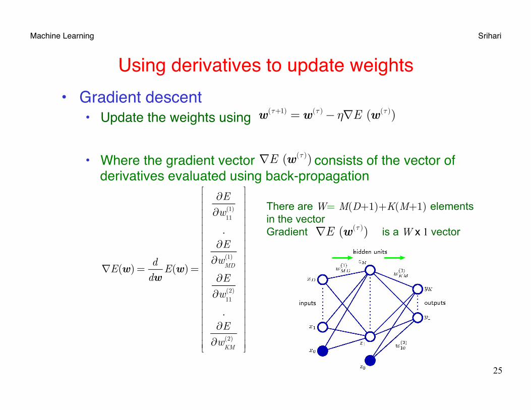
Using derivatives to update weights•  Gradient descent

•  Update the weights using

•  Where the gradient vector consists of the vector of derivatives evaluated using back-propagation

25

w(τ+1) = w(τ)− η∇E (w(τ))

∇E (w(τ))

∇E(w) =d

dwE(w) =

∂E∂w

11(1)

.∂E∂w

MD(1)

∂E∂w

11(2)

.∂E∂w

KM(2)

⎡

⎣

⎢⎢⎢⎢⎢⎢⎢⎢⎢⎢⎢⎢⎢⎢⎢⎢⎢⎢⎢⎢

⎤

⎦

⎥⎥⎥⎥⎥⎥⎥⎥⎥⎥⎥⎥⎥⎥⎥⎥⎥⎥⎥⎥

There are W= M(D+1)+K(M+1) elements in the vector Gradient is a W x 1 vector ∇E (w(τ))

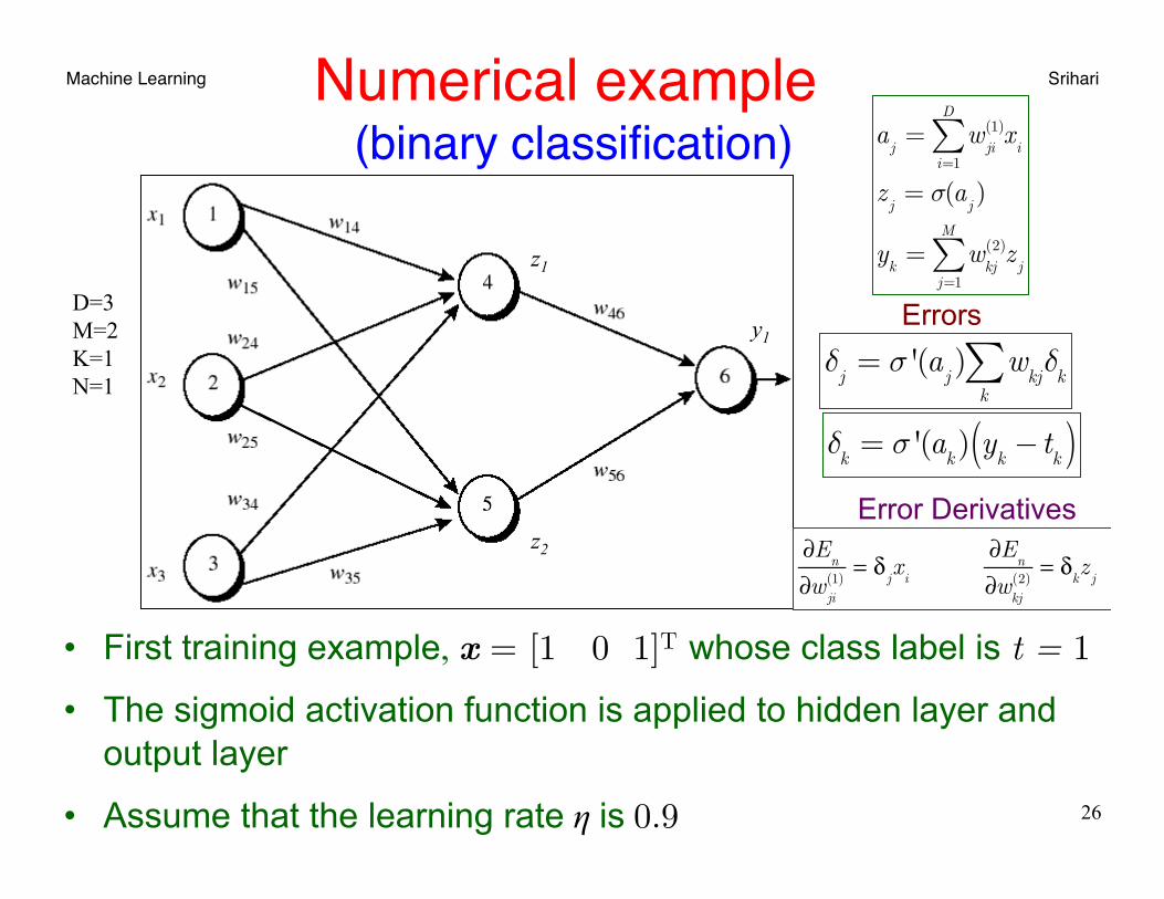
Machine Learning Srihari Numerical example (binary classification)

26

•  First training example, x = [1 0 1]T whose class label is t = 1

•  The sigmoid activation function is applied to hidden layer and output layer

•  Assume that the learning rate η is 0.9

D=3 M=2 K=1 N=1

δj

= σ '(aj) w

kjk∑ δ

k

aj

= wji(1)

i=1

D

∑ xi

zj

= σ(aj)

yk

= wkj(2)

j=1

M

∑ zj

z2

z1

y1 Errors

δ

k= σ '(a

k) y

k− t

k( )Error Derivatives

∂En

∂wji(1)

= δjx

i

∂En

∂wkj(2)

= δkz

j

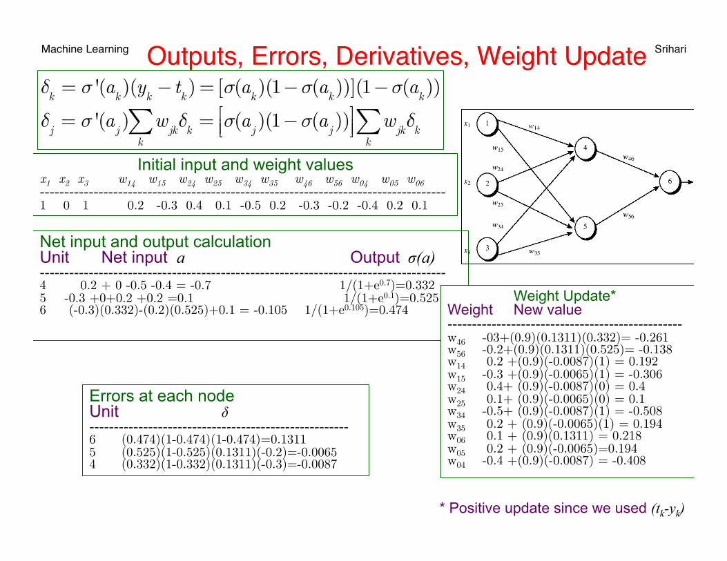
Machine Learning Srihari Outputs, Errors, Derivatives, Weight Update

δk

= σ '(ak)(y

k− t

k) = [σ(a

k)(1−σ(a

k))](1−σ(a

k))

δj

= σ '(aj) w

jkk∑ δ

k= σ(a

j)(1−σ(a

j))⎡

⎣⎢⎤⎦⎥ w

jkk∑ δ

k

Initial input and weight values x1 x2 x3 w14 w15 w24 w25 w34 w35 w46 w56 w04 w05 w06 ----------------------------------------------------------------------------------- 1 0 1 0.2 -0.3 0.4 0.1 -0.5 0.2 -0.3 -0.2 -0.4 0.2 0.1

Net input and output calculation Unit Net input a Output σ(a) ----------------------------------------------------------------------------------- 4 0.2 + 0 -0.5 -0.4 = -0.7 1/(1+e0.7)=0.332 5  -0.3 +0+0.2 +0.2 =0.1 1/(1+e0.1)=0.525 6  (-0.3)(0.332)-(0.2)(0.525)+0.1 = -0.105 1/(1+e0.105)=0.474

Errors at each node Unit δ ----------------------------------------------------- 6 (0.474)(1-0.474)(1-0.474)=0.1311 5 (0.525)(1-0.525)(0.1311)(-0.2)=-0.0065 4 (0.332)(1-0.332)(0.1311)(-0.3)=-0.0087

Weight Update* Weight New value ------------------------------------------------ w46 -03+(0.9)(0.1311)(0.332)= -0.261 w56 -0.2+(0.9)(0.1311)(0.525)= -0.138 w14 0.2 +(0.9)(-0.0087)(1) = 0.192 w15 -0.3 +(0.9)(-0.0065)(1) = -0.306 w24 0.4+ (0.9)(-0.0087)(0) = 0.4 w25 0.1+ (0.9)(-0.0065)(0) = 0.1 w34 -0.5+ (0.9)(-0.0087)(1) = -0.508 w35 0.2 + (0.9)(-0.0065)(1) = 0.194 w06 0.1 + (0.9)(0.1311) = 0.218 w05 0.2 + (0.9)(-0.0065)=0.194 w04 -0.4 +(0.9)(-0.0087) = -0.408

* Positive update since we used (tk-yk)

Machine Learning Srihari

MATLAB Implementation (Pseudocode)

•  Allows for multiple hidden layers •  Allows for training in batches •  Determines gradients using back-propagation using sum-

of-squared error •  Determines misclassification probability

Machine Learning

Srihari 28

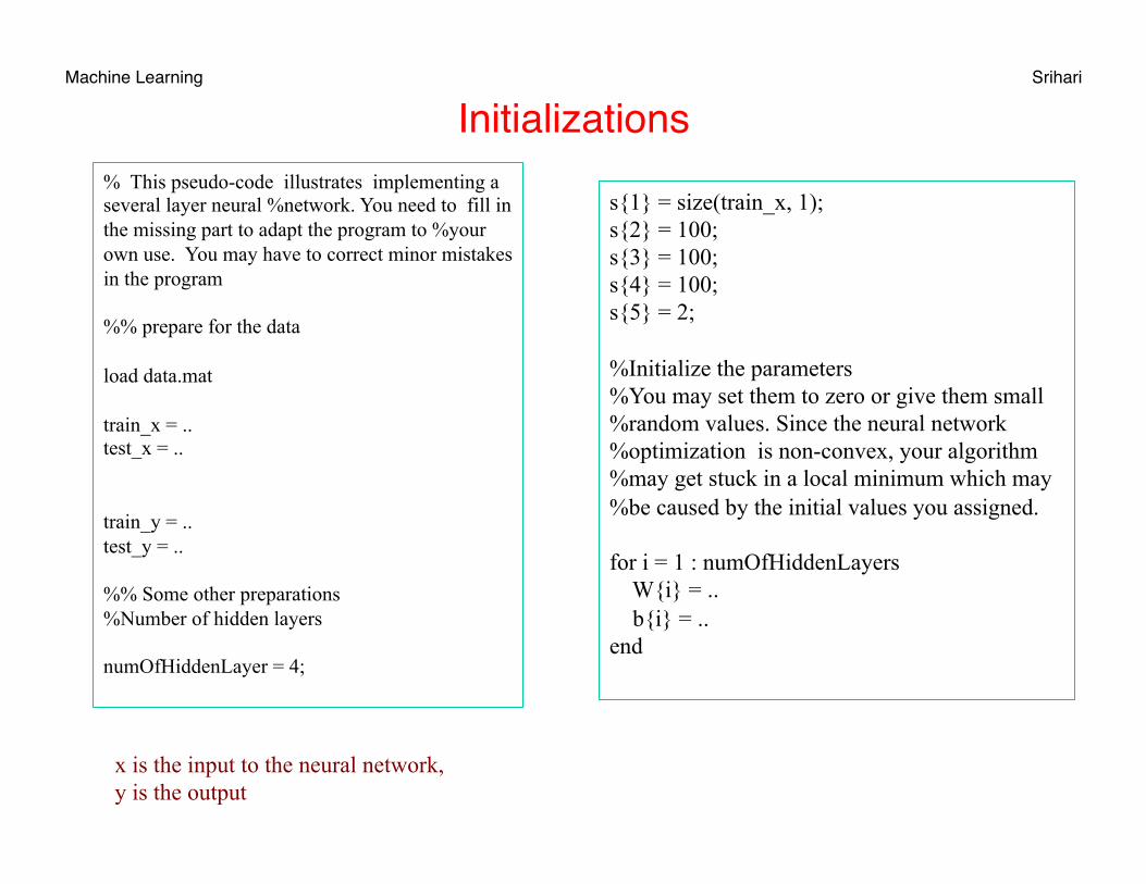
Machine Learning Srihari Initializations

% This pseudo-code illustrates implementing a several layer neural %network. You need to fill in the missing part to adapt the program to %your own use. You may have to correct minor mistakes in the program %% prepare for the data load data.mat train_x = .. test_x = .. train_y = .. test_y = .. %% Some other preparations %Number of hidden layers numOfHiddenLayer = 4;

s{1} = size(train_x, 1); s{2} = 100; s{3} = 100; s{4} = 100; s{5} = 2; %Initialize the parameters %You may set them to zero or give them small %random values. Since the neural network %optimization is non-convex, your algorithm %may get stuck in a local minimum which may %be caused by the initial values you assigned. for i = 1 : numOfHiddenLayers W{i} = .. b{i} = .. end

x is the input to the neural network, y is the output

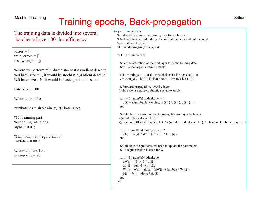
Machine Learning Srihari Training epochs, Back-propagation

losses = []; train_errors = []; test_wrongs = []; %Here we perform mini-batch stochastic gradient descent %If batchsize = 1, it would be stochastic gradient descent %If batchsize = N, it would be basic gradient descent batchsize = 100; %Num of batches numbatches = size(train_x, 2) / batchsize; %% Training part %Learning rate alpha alpha = 0.01; %Lambda is for regularization lambda = 0.001; %Num of iterations numepochs = 20;

for j = 1 : numepochs %randomly rearrange the training data for each epoch %We keep the shuffled index in kk, so that the input and output could %be matched together kk = randperm(size(train_x, 2)); for l = 1 : numbatches %Set the activation of the first layer to be the training data %while the target is training labels a{1} = train_x(:, kk( (l-1)*batchsize+1 : l*batchsize ) ); y = train_y(:, kk( (l-1)*batchsize+1 : l*batchsize ) ); %Forward propagation, layer by layer %Here we use sigmoid function as an example for i = 2 : numOfHiddenLayer + 1 a{i} = sigm( bsxfun(@plus, W{i-1}*a{i-1}, b{i-1}) ); end %Calculate the error and back-propagate error layer by layers d{numOfHiddenLayer + 1} = -(y - a{numOfHiddenLayer + 1}) .* a{numOfHiddenLayer + 1} .* (1-a{numOfHiddenLayer + 1}); for i = numOfHiddenLayer : -1 : 2 d{i} = W{i}' * d{i+1} .* a{i} .* (1-a{i}); end %Calculate the gradients we need to update the parameters %L2 regularization is used for W for i = 1 : numOfHiddenLayer dW{i} = d{i+1} * a{i}’; db{i} = sum(d{i+1}, 2); W{i} = W{i} - alpha * (dW{i} + lambda * W{i}); b{i} = b{i} - alpha * db{i}; end end

The training data is divided into several batches of size 100 for efficiency

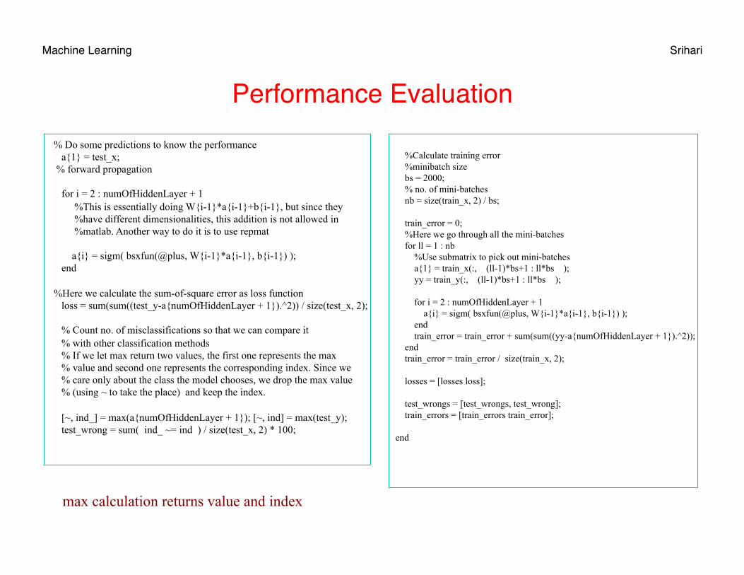
Machine Learning Srihari

Performance Evaluation % Do some predictions to know the performance a{1} = test_x; % forward propagation for i = 2 : numOfHiddenLayer + 1 %This is essentially doing W{i-1}*a{i-1}+b{i-1}, but since they %have different dimensionalities, this addition is not allowed in %matlab. Another way to do it is to use repmat a{i} = sigm( bsxfun(@plus, W{i-1}*a{i-1}, b{i-1}) ); end %Here we calculate the sum-of-square error as loss function loss = sum(sum((test_y-a{numOfHiddenLayer + 1}).^2)) / size(test_x, 2); % Count no. of misclassifications so that we can compare it % with other classification methods % If we let max return two values, the first one represents the max % value and second one represents the corresponding index. Since we % care only about the class the model chooses, we drop the max value % (using ~ to take the place) and keep the index. [~, ind_] = max(a{numOfHiddenLayer + 1}); [~, ind] = max(test_y); test_wrong = sum( ind_ ~= ind ) / size(test_x, 2) * 100;

%Calculate training error %minibatch size bs = 2000; % no. of mini-batches nb = size(train_x, 2) / bs; train_error = 0; %Here we go through all the mini-batches for ll = 1 : nb %Use submatrix to pick out mini-batches a{1} = train_x(:, (ll-1)*bs+1 : ll*bs ); yy = train_y(:, (ll-1)*bs+1 : ll*bs ); for i = 2 : numOfHiddenLayer + 1 a{i} = sigm( bsxfun(@plus, W{i-1}*a{i-1}, b{i-1}) ); end train_error = train_error + sum(sum((yy-a{numOfHiddenLayer + 1}).^2)); end train_error = train_error / size(train_x, 2); losses = [losses loss]; test_wrongs = [test_wrongs, test_wrong]; train_errors = [train_errors train_error]; end

max calculation returns value and index

Machine Learning Srihari

Efficiency of Backpropagation•  Computational Efficiency is main aspect of back-prop•  No of operations to compute derivatives of error function scales

with total number W of weights and biases•  Single evaluation of error function for a single input requires

O(W) operations (for large W)•  This is in contrast to O(W2) for numerical differentiation

•  As seen next

32

Machine Learning Srihari

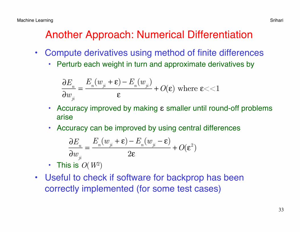
Another Approach: Numerical Differentiation•  Compute derivatives using method of finite differences

•  Perturb each weight in turn and approximate derivatives by

•  Accuracy improved by making ε smaller until round-off problems arise

•  Accuracy can be improved by using central differences

•  This is O(W2)

•  Useful to check if software for backprop has been correctly implemented (for some test cases)

33

∂En

∂wji

=E

n(w

ji+ ε)− E

n(w

ji)

ε+O(ε) where ε<<1

∂En

∂wji

=E

n(w

ji+ ε)− E

n(w

ji− ε)

2ε+O(ε2)

Machine Learning Srihari

Summary of Backpropagation

•  Derivatives of error function wrt weights are obtained by propagating errors backward

•  It is more efficient than numerical differentiation•  It can also be used for other computations

•  As seen next for Jacobian

34

Machine Learning Srihari

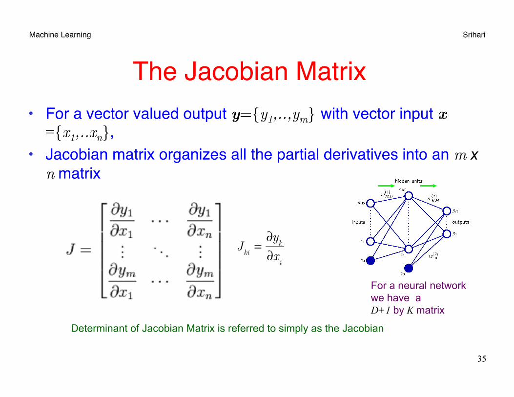
The Jacobian Matrix•  For a vector valued output y={y1,..,ym} with vector input x

={x1,..xn}, •  Jacobian matrix organizes all the partial derivatives into an m x

n matrix

35

J

ki=∂y

k

∂xi

Determinant of Jacobian Matrix is referred to simply as the Jacobian

For a neural network we have a D+1 by K matrix

Machine Learning Srihari

Jacobian Matrix Evaluation•  In backprop, derivatives of error function wrt weights are

obtained by propagating errors backwards through the network

•  The technique of backpropagation can also be used to calculate other derivatives

•  Here we consider the Jacobian matrix•  Whose elements are derivatives of network outputs wrt inputs

•  Where each such derivative is evaluated with other inputs fixed

36

J

ki=∂y

k

∂xi

Machine Learning Srihari

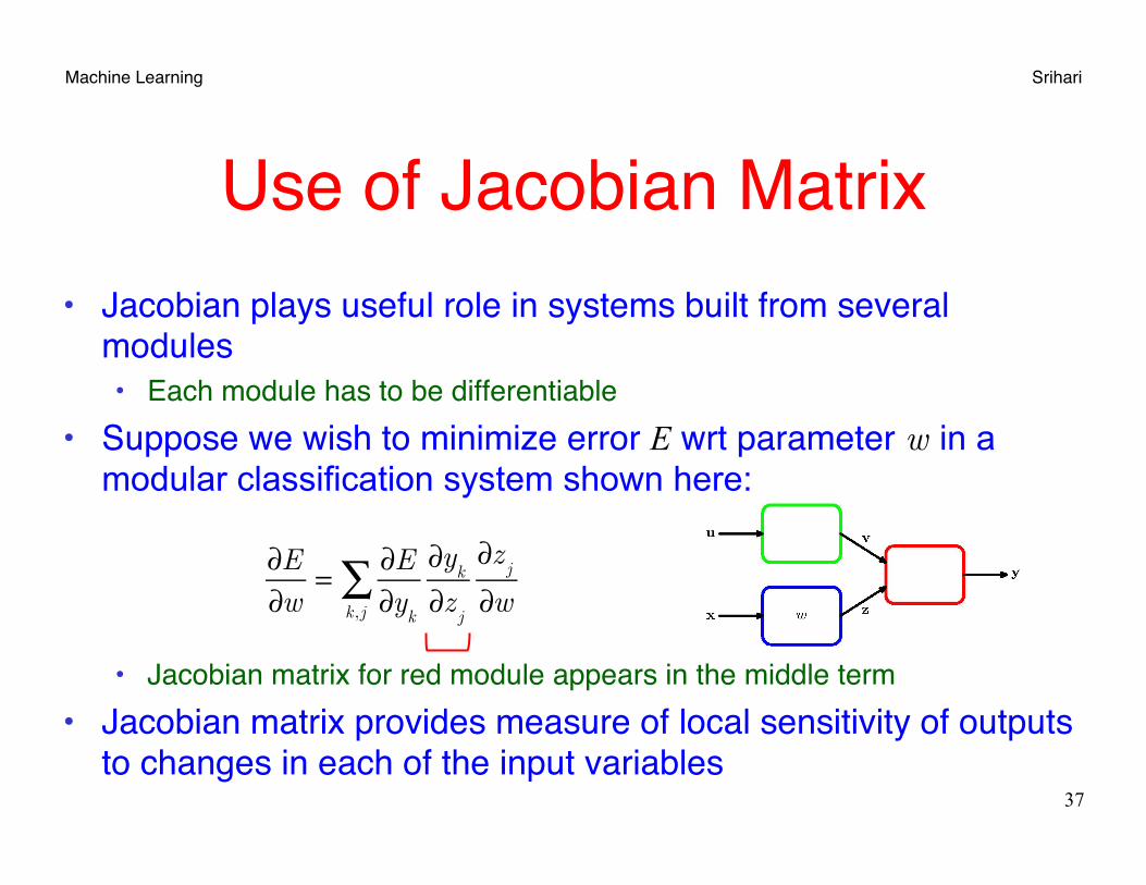
Use of Jacobian Matrix•  Jacobian plays useful role in systems built from several

modules•  Each module has to be differentiable

•  Suppose we wish to minimize error E wrt parameter w in a modular classification system shown here:

•  Jacobian matrix for red module appears in the middle term•  Jacobian matrix provides measure of local sensitivity of outputs

to changes in each of the input variables37

∂E∂w

= ∂E∂y

kk,j∑ ∂y

k

∂zj

∂zj

∂w

Machine Learning Srihari

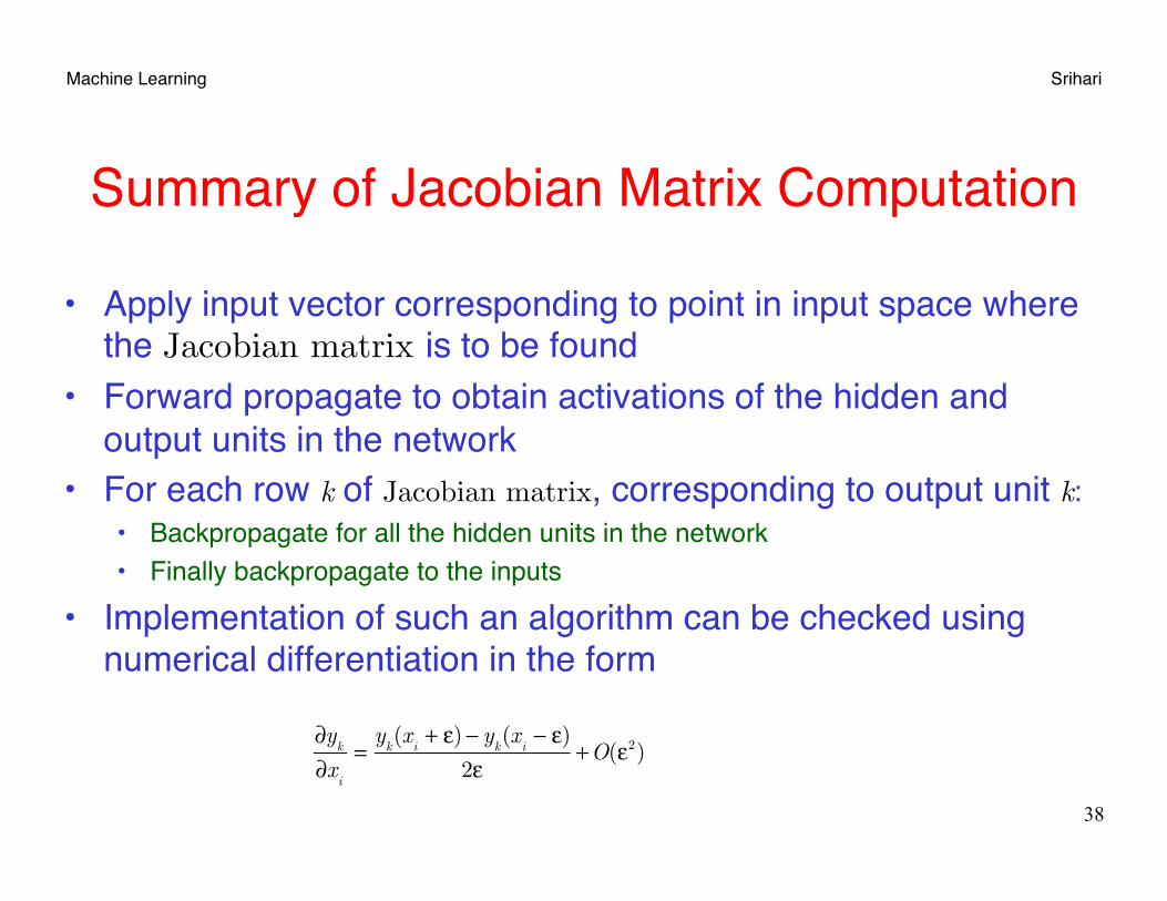
Summary of Jacobian Matrix Computation

•  Apply input vector corresponding to point in input space where the Jacobian matrix is to be found

•  Forward propagate to obtain activations of the hidden and output units in the network

•  For each row k of Jacobian matrix, corresponding to output unit k:•  Backpropagate for all the hidden units in the network•  Finally backpropagate to the inputs

•  Implementation of such an algorithm can be checked using numerical differentiation in the form

38

∂yk

∂xi

=y

k(x

i+ ε)− y

k(x

i− ε)

2ε+O(ε2)

Machine Learning Srihari Summary

•  Neural network learning needs learning of weights from samples involves two steps: •  Determine derivative of output of a unit wrt each input•  Adjust weights using derivatives

•  Backpropagation is a general term for computing derivatives•  Evaluate δk for all output units

•  (using δk=yk-tk for regression)•  Backpropagate the δk’s to obtain δj for each hidden unit•  Product of δ’s with activations at the unit provide the derivatives for that

weight•  Backpropagation is also useful to compute a Jacobian matrix

with several inputs and outputs•  Jacobian matrices are useful to determine the effects of different inputs

39