Vacuum Instabilities with a Wrong-Sign Higgs-Gluon-Gluon ...
20
Vacuum Instabilities with a Wrong-Sign Higgs-Gluon-Gluon Amplitude Matthew Reece [email protected] Department of Physics, Harvard University, Cambridge, MA 02138 November 1, 2018 Abstract The recently discovered 125 GeV boson appears very similar to a Standard Model Higgs, but with data favoring an enhanced h → γγ rate. A number of groups have found that fits would allow (or, less so after the latest updates, prefer) that the ht ¯ t coupling have the opposite sign. This can be given meaning in the context of an electroweak chiral Lagrangian, but it might also be interpreted to mean that a new colored and charged particle runs in loops and produces the opposite-sign hGG amplitude to that generated by integrating out the top, as well as a contribution reinforcing the W - loop contribution to hFF . In order to not suppress the rate of h → WW and h → ZZ , which appear to be approximately Standard Model-like, one would need the loop to “overshoot,” not only canceling the top contribution but producing an opposite-sign hGG vertex of about the same magnitude as that in the SM. We argue that most such explanations have severe problems with fine-tuning and, more importantly, vacuum stability. In particular, the case of stop loops producing an opposite-sign hGG vertex of the same size as the Standard Model one is ruled out by a combination of vacuum decay bounds and LEP constraints. We also show that scenarios with a sign flip from loops of color octet charged scalars or new fermionic states are highly constrained. 1 Introduction The Higgs discovery represents a major milestone in particle physics [1,2]. It brings renewed urgency to the question of naturalness: if the Higgs has precisely the properties predicted by the Standard Model, we may be forced to confront the possibility that we live in what is, to all appearances, a finely-tuned world. The experimental results so far present us with tantalizing hints that σ × Br(h → γγ) may be substantially larger than the Standard Model prediction [3,4]. Indeed, a number of groups of theorists have attempted to fit the data allowing for non-Standard-Model Higgs couplings, both before [5–15] and after [16–24] the July 4, 2012 discovery announcement. Although many details of the fits and the allowed parameter space are explained in these references, we can summarize the situation (keeping in mind that the error bars are still rather large) by saying that the Higgs σ × Br to WW and ZZ is essentially consistent with the Standard Model, the rate to γγ is somewhat high, and the rate to τ leptons may be low although Tevatron results suggest that the b-quark rate is not very suppressed. In almost every way, the Higgs appears to be nearly Standard- Model-like. Nonetheless, fits of the Higgs couplings allow (or even, less so after recent ATLAS h → WW results, favor) a region with R t = -1, i.e. a flipped sign of the Higgs–top–top coupling. This sign is fixed in the Standard Model without higher-dimension operators, but can be altered in the electroweak 1 arXiv:1208.1765v2 [hep-ph] 23 Oct 2012
Transcript of Vacuum Instabilities with a Wrong-Sign Higgs-Gluon-Gluon ...
Vacuum Instabilities with a Wrong-Sign Higgs-Gluon-GluonAmplitude
Matthew [email protected]
Department of Physics, Harvard University, Cambridge, MA 02138
November 1, 2018
Abstract
The recently discovered 125 GeV boson appears very similar to a Standard Model Higgs, butwith data favoring an enhanced h→ γγ rate. A number of groups have found that fits would allow(or, less so after the latest updates, prefer) that the ht t coupling have the opposite sign. This can begiven meaning in the context of an electroweak chiral Lagrangian, but it might also be interpretedto mean that a new colored and charged particle runs in loops and produces the opposite-sign hGGamplitude to that generated by integrating out the top, as well as a contribution reinforcing the W -loop contribution to hF F . In order to not suppress the rate of h→WW and h→ Z Z , which appear tobe approximately Standard Model-like, one would need the loop to “overshoot,” not only cancelingthe top contribution but producing an opposite-sign hGG vertex of about the same magnitude asthat in the SM. We argue that most such explanations have severe problems with fine-tuning and,more importantly, vacuum stability. In particular, the case of stop loops producing an opposite-signhGG vertex of the same size as the Standard Model one is ruled out by a combination of vacuumdecay bounds and LEP constraints. We also show that scenarios with a sign flip from loops of coloroctet charged scalars or new fermionic states are highly constrained.
1 Introduction
The Higgs discovery represents a major milestone in particle physics [1,2]. It brings renewed urgency tothe question of naturalness: if the Higgs has precisely the properties predicted by the Standard Model,we may be forced to confront the possibility that we live in what is, to all appearances, a finely-tunedworld. The experimental results so far present us with tantalizing hints that σ× Br(h→ γγ) may besubstantially larger than the Standard Model prediction [3,4]. Indeed, a number of groups of theoristshave attempted to fit the data allowing for non-Standard-Model Higgs couplings, both before [5–15]and after [16–24] the July 4, 2012 discovery announcement.
Although many details of the fits and the allowed parameter space are explained in these references,we can summarize the situation (keeping in mind that the error bars are still rather large) by sayingthat the Higgs σ × Br to WW and Z Z is essentially consistent with the Standard Model, the rate toγγ is somewhat high, and the rate to τ leptons may be low although Tevatron results suggest that theb-quark rate is not very suppressed. In almost every way, the Higgs appears to be nearly Standard-Model-like. Nonetheless, fits of the Higgs couplings allow (or even, less so after recent ATLAS h→WWresults, favor) a region with Rt = −1, i.e. a flipped sign of the Higgs–top–top coupling. This sign isfixed in the Standard Model without higher-dimension operators, but can be altered in the electroweak
1
arX
iv:1
208.
1765
v2 [
hep-
ph]
23
Oct
201
2
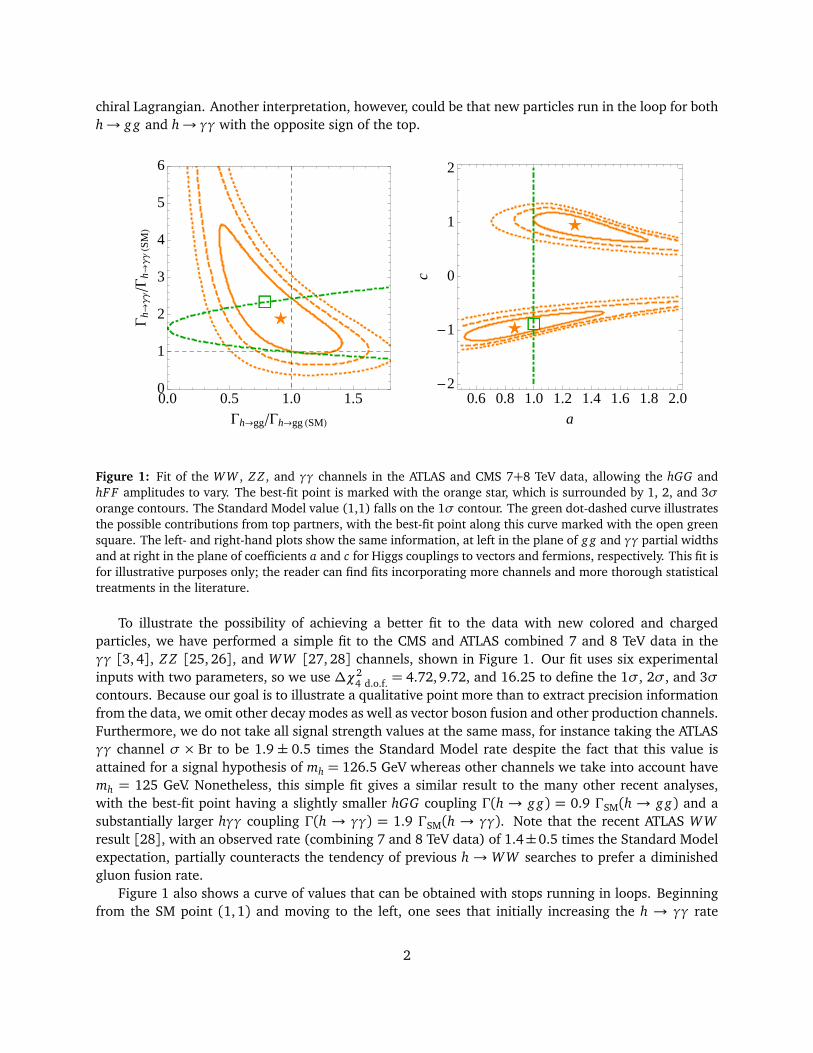
chiral Lagrangian. Another interpretation, however, could be that new particles run in the loop for bothh→ g g and h→ γγ with the opposite sign of the top.
øøáá
0.0 0.5 1.0 1.50
1
2
3
4
5
6
Gh®gg�Gh®gg HSML
Gh®
ΓΓ�G
h®ΓΓ
HSM
L øø
øø áá
0.6 0.8 1.0 1.2 1.4 1.6 1.8 2.0-2
-1
0
1
2
ac
Figure 1: Fit of the WW , Z Z , and γγ channels in the ATLAS and CMS 7+8 TeV data, allowing the hGG andhF F amplitudes to vary. The best-fit point is marked with the orange star, which is surrounded by 1, 2, and 3σorange contours. The Standard Model value (1,1) falls on the 1σ contour. The green dot-dashed curve illustratesthe possible contributions from top partners, with the best-fit point along this curve marked with the open greensquare. The left- and right-hand plots show the same information, at left in the plane of g g and γγ partial widthsand at right in the plane of coefficients a and c for Higgs couplings to vectors and fermions, respectively. This fit isfor illustrative purposes only; the reader can find fits incorporating more channels and more thorough statisticaltreatments in the literature.
To illustrate the possibility of achieving a better fit to the data with new colored and chargedparticles, we have performed a simple fit to the CMS and ATLAS combined 7 and 8 TeV data in theγγ [3, 4], Z Z [25, 26], and WW [27, 28] channels, shown in Figure 1. Our fit uses six experimentalinputs with two parameters, so we use ∆χ2
4 d.o.f. = 4.72,9.72, and 16.25 to define the 1σ, 2σ, and 3σcontours. Because our goal is to illustrate a qualitative point more than to extract precision informationfrom the data, we omit other decay modes as well as vector boson fusion and other production channels.Furthermore, we do not take all signal strength values at the same mass, for instance taking the ATLASγγ channel σ × Br to be 1.9 ± 0.5 times the Standard Model rate despite the fact that this value isattained for a signal hypothesis of mh = 126.5 GeV whereas other channels we take into account havemh = 125 GeV. Nonetheless, this simple fit gives a similar result to the many other recent analyses,with the best-fit point having a slightly smaller hGG coupling Γ(h → g g) = 0.9 ΓSM(h → g g) and asubstantially larger hγγ coupling Γ(h → γγ) = 1.9 ΓSM(h → γγ). Note that the recent ATLAS WWresult [28], with an observed rate (combining 7 and 8 TeV data) of 1.4±0.5 times the Standard Modelexpectation, partially counteracts the tendency of previous h→ WW searches to prefer a diminishedgluon fusion rate.
Figure 1 also shows a curve of values that can be obtained with stops running in loops. Beginningfrom the SM point (1,1) and moving to the left, one sees that initially increasing the h → γγ rate
2
decreases the h→ g g rate, but at a certain point the curve turns around and both rates increase. Thiscorresponds to reversing the sign of the hGG amplitude. The best-fit point on the curve has Γ(h →g g) = 0.8 ΓSM(h→ g g) (but with an amplitude of opposite sign) and Γ(h→ γγ) = 2.3 ΓSM(h→ γγ).A similar observation appeared recently in Ref. [18]. However, it is important to realize that this is avery large loop effect, inverting the sign of the hGG amplitude from a top loop by subtracting a newcontribution twice as large. Such large loop effects are not expected in the “natural SUSY” scenario thatoften motivates consideration of light stops [29, 30], and are not innocuous. In particular, the sameparticles that run in these loops affect the Higgs potential, and if they are scalars, they have a potentialof their own with possible new minima. We will argue that these effects are not benign, and trying touse the upper branch of the green curve in Figure 1 to explain the data brings with it a host of newproblems, whether the new particles are scalars or fermions.
2 Loop effects of charged and colored particles
2.1 Computing the effects
New particles that obtain a portion of their mass from the Higgs boson also alter the Higgs potential.We will be primarily concerned with their effect on the Higgs quartic, which determines the mass ofthe Higgs boson once the appropriate vacuum is found. To compute the shift in the quartic, we use theone-loop Coleman-Weinberg potential,
VCW =1
32π2
∑
(−1)FM 4
�
logM 2
µ2 −3
2
�
, (1)
expressing the mass of the new particles in terms of the Higgs field H, expanding as a function ofH, and reading off the coefficient of |H|4 to obtain a correction δλ to the quartic. Note that whenexpanding around the origin and reading off the |H|4 term, we neglect possible |H|4 log |H|2 terms thatwould arise from fields that are massless when the Higgs has no vev. Because we are interested innegative contributions to the hGG coupling, the dominant effect of increasing the Higgs vev should beto decrease the mass of the fields we integrate out, and this is a reasonable approximation to use.
Corrections to the effective Higgs couplings to photons and gluons are easily understood in terms ofthe low-energy theorem [31,32]. Namely, to read off the effective coupling induced by integrating outheavy particles, one treats them as a Higgs-dependent mass threshold in the beta function, obtainingthe effective vertex from the running of 1/g2:
−1
4g2 GaµνGaµν ⊃−
1
4
�
−∆b
16π2 logdet M2(h)�
GaµνGaµν ⊃
∆b
64π2
h
vGaµνGaµν ∂ logdet M2
∂ log v. (2)
with ∆b the beta function coefficient of the states that were integrated out. An analogous statementholds for couplings to photons, the only difference being that it is the electromagnetic beta functioncoefficient that appears. In the case that the mass of the new particles is not much greater than halfthe Higgs mass, it can be important to take into account mass-dependent corrections to the low-energy
theorem. In particular, for fermions these corrections are 1+7m2
h
120m2F+ O (m4
h/m4F ) and for scalars 1+
2m2h
15m2S+O (m4
h/m4S).
3
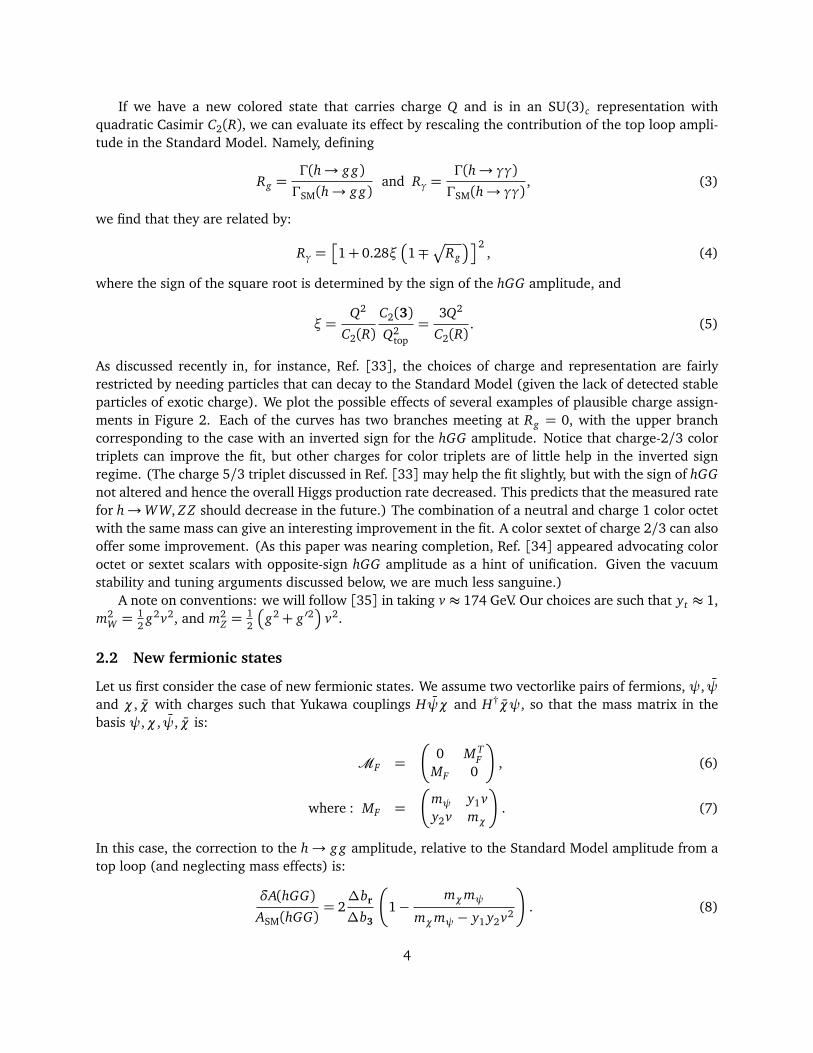
If we have a new colored state that carries charge Q and is in an SU(3)c representation withquadratic Casimir C2(R), we can evaluate its effect by rescaling the contribution of the top loop ampli-tude in the Standard Model. Namely, defining
Rg =Γ(h→ g g)ΓSM(h→ g g)
and Rγ =Γ(h→ γγ)ΓSM(h→ γγ)
, (3)
we find that they are related by:
Rγ =�
1+ 0.28ξ�
1∓p
Rg
��2, (4)
where the sign of the square root is determined by the sign of the hGG amplitude, and
ξ=Q2
C2(R)C2(3)Q2
top
=3Q2
C2(R). (5)
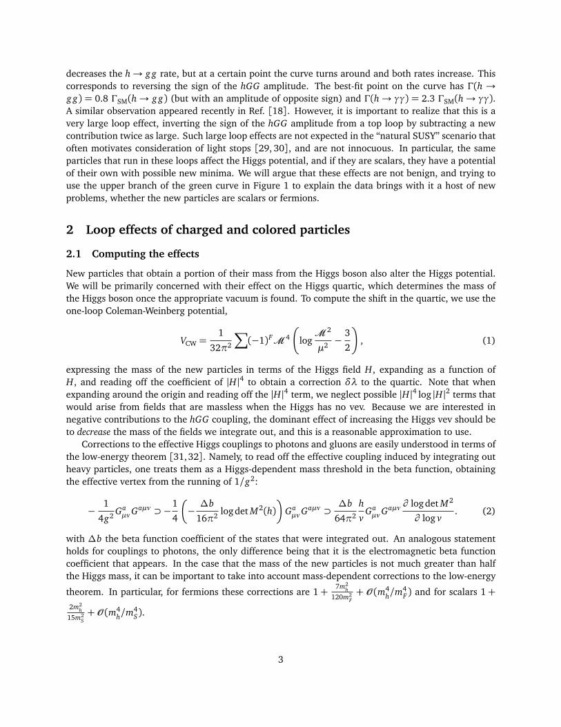
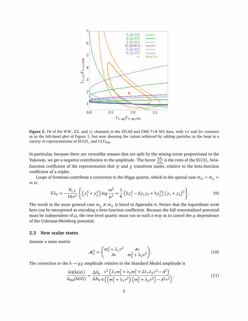
As discussed recently in, for instance, Ref. [33], the choices of charge and representation are fairlyrestricted by needing particles that can decay to the Standard Model (given the lack of detected stableparticles of exotic charge). We plot the possible effects of several examples of plausible charge assign-ments in Figure 2. Each of the curves has two branches meeting at Rg = 0, with the upper branchcorresponding to the case with an inverted sign for the hGG amplitude. Notice that charge-2/3 colortriplets can improve the fit, but other charges for color triplets are of little help in the inverted signregime. (The charge 5/3 triplet discussed in Ref. [33]may help the fit slightly, but with the sign of hGGnot altered and hence the overall Higgs production rate decreased. This predicts that the measured ratefor h→WW, Z Z should decrease in the future.) The combination of a neutral and charge 1 color octetwith the same mass can give an interesting improvement in the fit. A color sextet of charge 2/3 can alsooffer some improvement. (As this paper was nearing completion, Ref. [34] appeared advocating coloroctet or sextet scalars with opposite-sign hGG amplitude as a hint of unification. Given the vacuumstability and tuning arguments discussed below, we are much less sanguine.)
A note on conventions: we will follow [35] in taking v ≈ 174 GeV. Our choices are such that yt ≈ 1,m2
W =12
g2v2, and m2Z =
12
�
g2+ g ′2�
v2.
2.2 New fermionic states
Let us first consider the case of new fermionic states. We assume two vectorlike pairs of fermions, ψ, ψand χ, χ with charges such that Yukawa couplings Hψχ and H†χψ, so that the mass matrix in thebasis ψ,χ, ψ, χ is:
MF =
�
0 M TF
MF 0
�
, (6)
where : MF =
�
mψ y1vy2v mχ
�
. (7)
In this case, the correction to the h→ g g amplitude, relative to the Standard Model amplitude from atop loop (and neglecting mass effects) is:
δA(hGG)ASM(hGG)
= 2∆br
∆b3
�
1−mχmψ
mχmψ− y1 y2v2
�
. (8)
4
øø
0.0 0.5 1.0 1.5
1
2
3
4
5
6
7
Gh®gg�Gh®gg HSML
Gh®
ΓΓ�G
h®ΓΓ
HSM
L
3, Q=2�33, Q=1�33, Q=5�38, Q=0+16, Q=4�36, Q=2�3
ø: Best Fit
Figure 2: Fit of the WW , Z Z , and γγ channels in the ATLAS and CMS 7+8 TeV data, with 1σ and 2σ contoursas in the left-hand plot of Figure 1, but now showing the values achieved by adding particles in the loop in avariety of representations of SU(3)c and U(1)EM.
In particular, because there are vectorlike masses that are split by the mixing terms proportional to theYukawas, we get a negative contribution to the amplitude. The factor ∆br
∆b3is the ratio of the SU(3)c beta-
function coefficient of the representation that ψ and χ transform under, relative to the beta-functioncoefficient of a triplet.
Loops of fermions contribute a correction to the Higgs quartic, which in the special case mψ = mχ =m is:
δλF =−Nc;F
16π2
¨
�
y41 + y4
2
�
logm2
µ2 +1
6
�
5y21 − 2y1 y2+ 5y2
2
�
�
y1+ y2�2
«
. (9)
The result in the more general case mχ 6= mψ is listed in Appendix A. Notice that the logarithmic termhere can be interpreted as encoding a beta function coefficient. Because the full renormalized potentialmust be independent of µ, the tree-level quartic must run in such a way as to cancel the µ-dependenceof the Coleman-Weinberg potential.
2.3 New scalar states
Assume a mass matrix
M 2S =
�
m21+λ1v2 Av
Av m22+λ2v2
�
. (10)
The correction to the h→ g g amplitude relative to the Standard Model amplitude is
δA(hGG)ASM(hGG)
=∆br
∆b3
v2�
λ1m22+λ2m2
1+ 2λ1λ2v2− A2�
4��
m21+λ1v2
��
m22+λ2v2
�
− A2v2� , (11)
5
The factor of 1/4 arises from the relative beta function coefficients of a single color-triplet scalar andthe top quark, whereas the factor ∆br
∆b3again corrects for the case when the field is not in the 3 of
SU(3)c . As in the case of fermions, the effect of mixing (here proportional to A) is to split the masseigenstates and thus give a negative contribution. On the other hand, the quartic couplings λ1,2 cangive contributions of either sign.
The correction to the Higgs quartic in the case where the mass parameters m1 and m2 are equal is:
δλS =Nc;S
32π2
�
(λ21+λ
22) log
m2
µ2 + (λ1+λ2)A2
m2 −1
6
A4
m4
�
. (12)
The result in the more general case m1 6= m2 is given in Appendix A. To compare to a more fa-miliar expression: if the scalar states are stops in a supersymmetric theory, we have m2
1 = m2Q3
,
m22 = m2
uc3, Nc;S = 3, λ1 = y2
t +�
12− 2
3sin2 θW
�
cos(2β) g2+g ′2
2, λ2 = y2
t +23
sin2 θW cos(2β) g2+g ′2
2,
and A= yt�
At sinβ −µ cosβ�
. In particular, the part of δλS that is polynomial in A, dropping terms oforder g2, taking m2
Q3= m2
uc3= m2
t , and assuming large enough tanβ , is:
δλS ≈3
16π2 y4t
X 2t
m2t
−1
12
X 4t
m4t
!
, (13)
with X t = At − µ cotβ . This is the familiar result that can be found in, for example, [36]. As for
the logarithmic term, tops contribute − 316π2 y4
t logm2
t
µ2 , so the µ-dependence cancels and the leftover
logarithmic correction is 316π2 y4
t logm2
t
m2t, which is also of the familiar expected form.
3 Vacuum stability
Given the results of the Coleman-Weinberg calculation, it is apparent that trying to achieve a largeenough loop correction to change the sign of the hGG coupling is a dangerous game. Flipping the signimplies having a particle with a mass that diminishes with increasing Higgs VEV. One possibility for thisis a mixing effect: either one has vectorlike fermions getting a majority of their mass independent ofthe Higgs, or scalars that mix analogously to the familiar case of stops in supersymmetric theories. Inthe case of fermions, the most dangerous effect is the renormalization group running from the fermionYukawa coupling, which pushes the Higgs quartic toward negative values in the UV and can lead toan unstable vacuum [37]. For scalars, the RG effect is not dangerous, as the Higgs quartic is pushedtoward larger values in the UV. However, there is a large negative threshold correction, proportionalto the fourth power of the mixing parameter A (familiar from the case of stops), which threatens tomake the Higgs tachyonic. Furthermore, such large mixing parameters can lead to color and chargebreaking minima of the tree-level potential [38]. The remaining alternative, which does not requirelarge mixings, is that one can have scalars with a positive mass2 and a negative quartic coupling tothe Higgs. Such a negative quartic coupling again can lead to color- and charge-breaking minima orrunaway directions. Our goal in this section is to give some simple estimates of the parameter spaceleading to catastrophic vacuum instabilities and show that most attempts to achieve an hGG couplingof approximately the Standard Model magnitude but opposite sign are ruled out by them.
6

3.1 Inverting hGG with Stops
Given that we are looking for large changes to the Higgs potential that require light new colored andcharged particles, it is reasonable to first consider whether stops can be responsible, since naturalnessof electroweak symmetry breaking in supersymmetric theories favors light stops [29, 30]. In the caseof stops, the general results discussed in the previous section imply a correction to the hGG amplitude(specializing the general result Eq. 11):
A(hGG)ASM(hGG)
= 1+1
4
m2t
m2t1
+m2
t
m2t2
−m2
t X 2t
m2t1
m2t2
, (14)
up to small D-term corrections (taken into account in the plots below). Here m t1and m t2
are masseigenvalues, not Lagrangian parameters. The effect of stops on Higgs branching ratios has been dis-cussed in several papers in the recent literature [6,17,18,24,39], which reach a variety of conclusions.As emphasized by Ref. [39], light unmixed stops tend to increase the hGG coupling and decrease thehγγ coupling, whereas highly mixed stops contribute large corrections to m2
Hu(thus requiring more
tuning for EWSB) and lead to large corrections to b → sγ that must also be tuned away. The sameconsiderations led Ref. [24] to focus on the “funnel” region in which the stop corrections to hGG aresmall. On the other hand, Refs. [18,22] argued for light and highly mixed stops in the region with theinverted sign of hGG, which could improve the fit to data.
2500
5000
7500
10 000
12 500
15 000
17 500
20 000
150
250
350
450
500 1000 1500 2000
500
1000
1500
2000
mQ
mU
Lightest Stop Mass and Xt
0.1
0.20.3 0.4
0.5
0.6
0.7
0.8
0.9750
1000
1250 1500
17502000
2250 2500
2750
500 1000 1500 2000
500
1000
1500
2000
mQ
mU
Heaviest Stop Mass and sin2Θt�
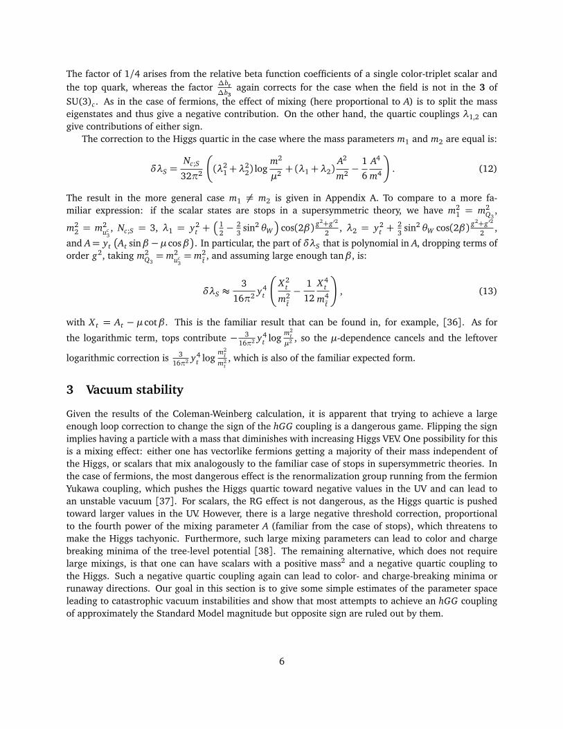
Figure 3: Stop parameter space that achieves a hGG coupling that is −1 times its Standard Model value. Thiscondition reduces the three-dimensional parameter space (mQ, mU , X t) to two dimensions, which we parametrizewith mQ and mU . At left: contours of the lightest stop mass (orange, dashed) and the value of X t needed toachieve the desired coupling (purple, solid). At right: contours of the heavy stop mass (orange, dashed) and thecorresponding stop mixing sin2 θ t parametrizing the right-handedness of the stop (purple, solid).
We illustrate the parameter space that can achieve A(hGG) = −ASM(hGG) in Figure 3. As is clearfrom equation 14, this occurs at very large values of the mixing parameter X t . This leads to a large
7
splitting between the two stop mass eigenstates. In this region of parameter space, the lightest stopeigenvalue tends to be fairly light. For example, pushing the light eigenstate up to 450 GeV implies 20TeV A-terms, which is an enormously finely-tuned scenario, both from the point of view of electroweaksymmetry breaking and of b→ sγ. In fact, from the Coleman-Weinberg discussion in Section 2.3, onecan readily see that such large A-terms lead to very large negative threshold corrections to the Higgsmass. This implies the need for very large beyond-MSSM couplings of the Higgs boson that are capableof lifting its mass up to 125 GeV. When such couplings become large enough, it is difficult to imaginethat other Higgs properties remain unmodified, so that considering only stop-loop modifications to thepartial widths is dubious. On the other hand, one may wonder if the lower-left corner of the plot, witha light stop eigenstate, can fit the data, with large but no longer unreasonably large A-terms. It is stillrather tuned. Recent experimental searches for direct production of light stops [40–45] constrain muchof the stop parameter space with m t1
<∼ 500 GeV, but only for sufficiently light neutralinos. The more
squeezed regime will be probed by a combination of traditional missing-ET signatures [46–55] and spincorrelations [56], and even the case of R-parity violation may be constrained soon [57]. Nonetheless,for the moment, these considerations still allow as a logical possibility that light, highly mixed stopssignificantly alter the Higgs properties.
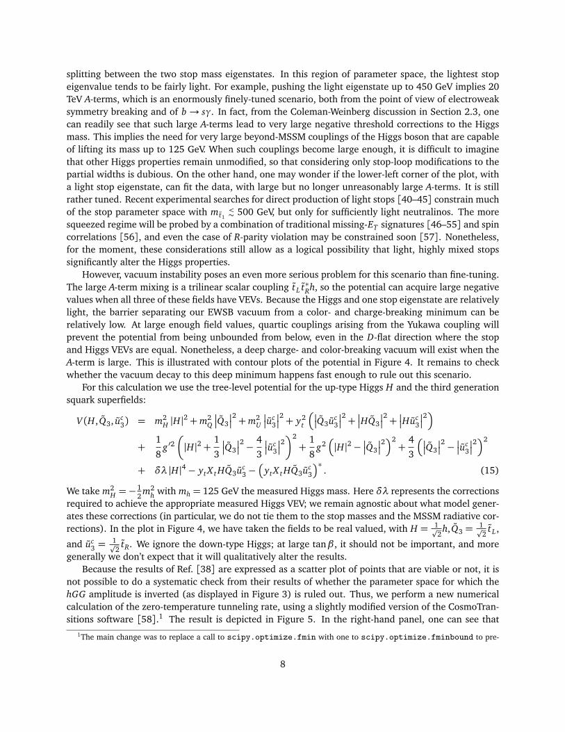
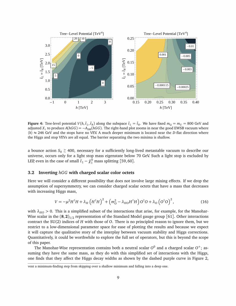
However, vacuum instability poses an even more serious problem for this scenario than fine-tuning.The large A-term mixing is a trilinear scalar coupling tL t∗Rh, so the potential can acquire large negativevalues when all three of these fields have VEVs. Because the Higgs and one stop eigenstate are relativelylight, the barrier separating our EWSB vacuum from a color- and charge-breaking minimum can berelatively low. At large enough field values, quartic couplings arising from the Yukawa coupling willprevent the potential from being unbounded from below, even in the D-flat direction where the stopand Higgs VEVs are equal. Nonetheless, a deep charge- and color-breaking vacuum will exist when theA-term is large. This is illustrated with contour plots of the potential in Figure 4. It remains to checkwhether the vacuum decay to this deep minimum happens fast enough to rule out this scenario.
For this calculation we use the tree-level potential for the up-type Higgs H and the third generationsquark superfields:
V (H, Q3, uc3) = m2
H |H|2+m2
Q
�
�Q3
�
�
2+m2
U
�
�uc3
�
�
2+ y2
t
�
�
�Q3uc3
�
�
2+�
�HQ3
�
�
2+�
�Huc3
�
�
2�
+1
8g ′2�
|H|2+1
3
�
�Q3
�
�
2−4
3
�
�uc3
�
�
2�2
+1
8g2�
|H|2−�
�Q3
�
�
2�2+
4
3
�
�
�Q3
�
�
2−�
�uc3
�
�
2�2
+ δλ |H|4− yt X t HQ3uc3−�
yt X t HQ3uc3
�∗. (15)
We take m2H =−
12m2
h with mh = 125 GeV the measured Higgs mass. Here δλ represents the correctionsrequired to achieve the appropriate measured Higgs VEV; we remain agnostic about what model gener-ates these corrections (in particular, we do not tie them to the stop masses and the MSSM radiative cor-rections). In the plot in Figure 4, we have taken the fields to be real valued, with H = 1p
2h, Q3 =
1p2
tL ,
and uc3 =
1p2
tR. We ignore the down-type Higgs; at large tanβ , it should not be important, and moregenerally we don’t expect that it will qualitatively alter the results.
Because the results of Ref. [38] are expressed as a scatter plot of points that are viable or not, it isnot possible to do a systematic check from their results of whether the parameter space for which thehGG amplitude is inverted (as displayed in Figure 3) is ruled out. Thus, we perform a new numericalcalculation of the zero-temperature tunneling rate, using a slightly modified version of the CosmoTran-sitions software [58].1 The result is depicted in Figure 5. In the right-hand panel, one can see that
1The main change was to replace a call to scipy.optimize.fmin with one to scipy.optimize.fminbound to pre-
8
-5
0
0
0
5
10
15
20
-1 0 1 2 30.0
0.5
1.0
1.5
2.0
2.5
3.0
h @TeVD
t� L=
t� R@T
eVD
Tree-Level Potential @TeV4D
-0.01
-0.005
-0.003
-0.00025-0.000115
0.001
0.15 0.20 0.25 0.30 0.35 0.400.00
0.05
0.10
0.15
0.20
0.25
h @TeVD
t� L=
t� R@T
eVD
Tree-Level Potential @TeV4D
Figure 4: Tree-level potential V (h, tL , tR) along the subspace tL = tR. We have fixed mQ = mU = 800 GeV andadjusted X t to produce A(hGG) =−ASM(hGG). The right-hand plot zooms in near the good EWSB vacuum where⟨h⟩ ≈ 246 GeV and the stops have no VEV. A much deeper minimum is located near the D-flat direction wherethe Higgs and stop VEVs are all equal. The barrier separating the two minima is shallow.
a bounce action S0>∼ 400, necessary for a sufficiently long-lived metastable vacuum to describe our
universe, occurs only for a light stop mass eigenstate below 70 GeV. Such a light stop is excluded byLEP, even in the case of small t1− χ0
1 mass splitting [59,60].
3.2 Inverting hGG with charged scalar color octets
Here we will consider a different possibility that does not involve large mixing effects. If we drop theassumption of supersymmetry, we can consider charged scalar octets that have a mass that decreaseswith increasing Higgs mass,
V =−µ2H†H +λH
�
H†H�2+�
m2O −λHOH†H
�
O†O+λO
�
O†O�2
, (16)
with λHO > 0. This is a simplified subset of the interactions that arise, for example, for the Manohar-Wise scalar in the (8,2)1/2 representation of the Standard Model gauge group [61]. Other interactionscontract the SU(2) indices of H with those of O. There is no principled reason to ignore them, but werestrict to a low-dimensional parameter space for ease of plotting the results and because we expectit will capture the qualitative story of the interplay between vacuum stability and Higgs corrections.Quantitatively, it could be worthwhile to explore the full set of operators, but this is beyond the scopeof this paper.
The Manohar-Wise representation contains both a neutral scalar O0 and a charged scalar O+; as-suming they have the same mass, as they do with this simplified set of interactions with the Higgs,one finds that they affect the Higgs decay widths as shown by the dashed purple curve in Figure 2,
vent a minimum-finding step from skipping over a shallow minimum and falling into a deep one.
9
5
10
2030
50
400 500 600 700 800 900 1000
400
500
600
700
800
900
1000
mQ @GeVD
mU
@GeV
DBounce Action
100
200
400
60 GeV 70 GeV
80 GeV
90 GeV
100 GeV
300 350 400 450
300
350
400
450
mQ @GeVD
mU
@GeV
D
Bounce Action
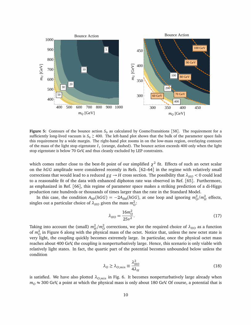
Figure 5: Contours of the bounce action S0 as calculated by CosmoTransitions [58]. The requirement for asufficiently long-lived vacuum is S0
>∼ 400. The left-hand plot shows that the bulk of the parameter space fails
this requirement by a wide margin. The right-hand plot zooms in on the low-mass region, overlaying contoursof the mass of the light stop eigenstate t1 (orange, dashed). The bounce action exceeds 400 only when the lightstop eigenstate is below 70 GeV, and thus cleanly excluded by LEP constraints.
which comes rather close to the best-fit point of our simplified χ2 fit. Effects of such an octet scalaron the hGG amplitude were considered recently in Refs. [62–64] in the regime with relatively smallcorrections that would lead to a reduced g g → H cross section. The possibility that λHO < 0 could leadto a reasonable fit of the data with enhanced diphoton rate was observed in Ref. [65]. Furthermore,as emphasized in Ref. [66], this regime of parameter space makes a striking prediction of a di-Higgsproduction rate hundreds or thousands of times larger than the rate in the Standard Model.
In this case, the condition ANP(hGG) = −2ASM(hGG), at one loop and ignoring m2O/m
2H effects,
singles out a particular choice of λHO given the mass m2O:
λHO =16m2
O
25v2 . (17)
Taking into account the (small) m2H/m
2O corrections, we plot the required choice of λHO as a function
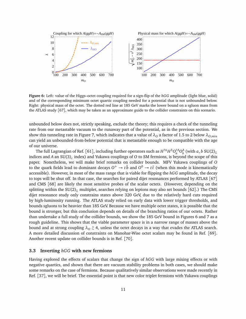
of m2O in Figure 6 along with the physical mass of the octet. Notice that, unless the new octet state is
very light, the coupling quickly becomes extremely large. In particular, once the physical octet massreaches about 400 GeV, the coupling is nonperturbatively large. Hence, this scenario is only viable withrelatively light states. In fact, the quartic part of the potential becomes unbounded below unless thecondition
λO ≥ λO;min ≡λ2
HO
4λH(18)
is satisfied. We have also plotted λO;min in Fig. 6. It becomes nonperturbatively large already whenmO ≈ 300 GeV, a point at which the physical mass is only about 180 GeV. Of course, a potential that is
10
100 200 300 400 500 600 7000
2
4
6
8
10
12
mO
Λ
Coupling for which AHggHL=-ASMHggHL
ΛO;min
ΛHO
100 200 300 400 500 600 700
100150200250300350400
mO
mO2
-v2
ΛH
O
Physical mass for which AHggHL=-ASMHggHL
Figure 6: Left: value of the Higgs–octet coupling required for a sign-flip of the hGG amplitude (light blue, solid)and of the corresponding minimum octet quartic coupling needed for a potential that is not unbounded below.Right: physical mass of the octet. The dotted red line at 185 GeV marks the lower bound on a sgluon mass fromthe ATLAS study [67], which may be taken as an approximate guide to the collider constraints on this scenario.
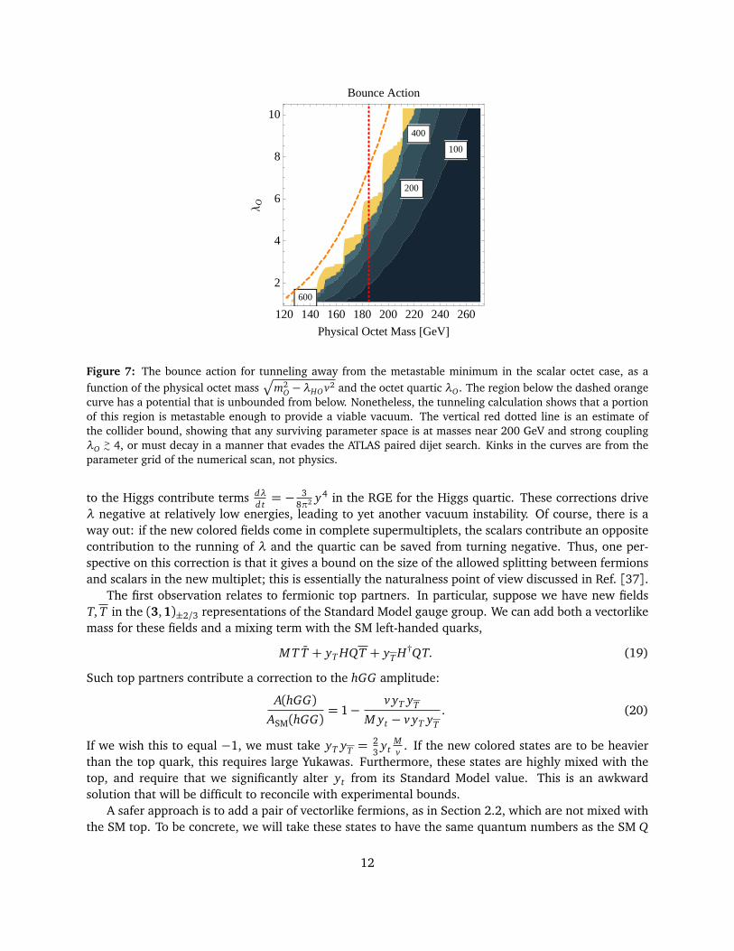
unbounded below does not, strictly speaking, exclude the theory; this requires a check of the tunnelingrate from our metastable vacuum to the runaway part of the potential, as in the previous section. Weshow this tunneling rate in Figure 7, which indicates that a value of λO a factor of 1.5 to 2 below λO;mincan yield an unbounded-from-below potential that is metastable enough to be compatible with the ageof our universe.
The full Lagrangian of Ref. [61], including further operators such as H†aH bO†Aa OA
b (with a, b SU(2)Lindices and A an SU(3)c index) and Yukawa couplings of O to SM fermions, is beyond the scope of thispaper. Nonetheless, we will make brief remarks on collider bounds. MFV Yukawa couplings of Oto the quark fields lead to dominant decays O+ → t b and O0 → t t (when this mode is kinematicallyaccessible). However, in most of the mass range that is viable for flipping the hGG amplitude, the decayto tops will be shut off. In that case, the searches for paired dijet resonances performed by ATLAS [67]and CMS [68] are likely the most sensitive probes of the scalar octets. (However, depending on thesplitting within the SU(2)L multiplet, searches relying on leptons may also set bounds [62].) The CMSdijet resonance study only constrains states above 320 GeV, due to the relatively hard cuts requiredby high-luminosity running. The ATLAS study relied on early data with lower trigger thresholds, andbounds sgluons to be heavier than 185 GeV. Because we have multiple octet states, it is possible that thebound is stronger, but this conclusion depends on details of the branching ratios of our octets. Ratherthan undertake a full study of the collider bounds, we show the 185 GeV bound in Figures 6 and 7 as arough guideline. This shows that the viable parameter space is in a narrow range of masses above thebound and at strong coupling λO
>∼ 4, unless the octet decays in a way that evades the ATLAS search.
A more detailed discussion of constraints on Manohar-Wise octet scalars may be found in Ref. [69].Another recent update on collider bounds is in Ref. [70].
3.3 Inverting hGG with new fermions
Having explored the effects of scalars that change the sign of hGG with large mixing effects or withnegative quartics, and shown that there are vacuum stability problems in both cases, we should makesome remarks on the case of fermions. Because qualitatively similar observations were made recently inRef. [37], we will be brief. The essential point is that new color triplet fermions with Yukawa couplings
11
100
200
400
600
120 140 160 180 200 220 240 260
2
4
6
8
10
Physical Octet Mass @GeVD
ΛO
Bounce Action
Figure 7: The bounce action for tunneling away from the metastable minimum in the scalar octet case, as afunction of the physical octet mass
p
m2O −λHO v2 and the octet quartic λO. The region below the dashed orange
curve has a potential that is unbounded from below. Nonetheless, the tunneling calculation shows that a portionof this region is metastable enough to provide a viable vacuum. The vertical red dotted line is an estimate ofthe collider bound, showing that any surviving parameter space is at masses near 200 GeV and strong couplingλO
>∼ 4, or must decay in a manner that evades the ATLAS paired dijet search. Kinks in the curves are from the
parameter grid of the numerical scan, not physics.
to the Higgs contribute terms dλd t= − 3
8π2 y4 in the RGE for the Higgs quartic. These corrections driveλ negative at relatively low energies, leading to yet another vacuum instability. Of course, there is away out: if the new colored fields come in complete supermultiplets, the scalars contribute an oppositecontribution to the running of λ and the quartic can be saved from turning negative. Thus, one per-spective on this correction is that it gives a bound on the size of the allowed splitting between fermionsand scalars in the new multiplet; this is essentially the naturalness point of view discussed in Ref. [37].
The first observation relates to fermionic top partners. In particular, suppose we have new fieldsT, T in the (3,1)±2/3 representations of the Standard Model gauge group. We can add both a vectorlikemass for these fields and a mixing term with the SM left-handed quarks,
M T T + yT HQT + yT H†QT. (19)
Such top partners contribute a correction to the hGG amplitude:
A(hGG)ASM(hGG)
= 1−v yT yT
M yt − v yT yT. (20)
If we wish this to equal −1, we must take yT yT =23
ytMv
. If the new colored states are to be heavierthan the top quark, this requires large Yukawas. Furthermore, these states are highly mixed with thetop, and require that we significantly alter yt from its Standard Model value. This is an awkwardsolution that will be difficult to reconcile with experimental bounds.
A safer approach is to add a pair of vectorlike fermions, as in Section 2.2, which are not mixed withthe SM top. To be concrete, we will take these states to have the same quantum numbers as the SM Q
12
and uc fields, but with a parity that prevents mixing terms with the SM. Furthermore, we will simplifythe story by taking mχ = mψ = M and y1 = y2 = y . Obtaining the amplitude A(hGG) = −ASM(hGG)then requires that y2v2 = 1
2M2, with mass eigenvalues about Mlight ≈ 0.29M and Mheavy ≈ 1.7M .
The finite correction to λ (which must have a value of about 0.13 for the correct Higgs VEV) from the
Coleman-Weinberg formula can then be expressed as − M4
4π2v4 ≈ −3.4M4
light
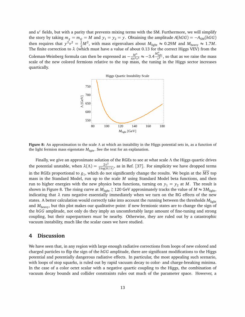
v4 , so that as we raise the massscale of the new colored fermions relative to the top mass, the tuning in the Higgs sector increasesquartically.
80 100 120 140 160 180
550
600
650
700
750
Mlight @GeVD
L@G
eVD
Higgs Quartic Instability Scale
Figure 8: An approximation to the scale Λ at which an instability in the Higgs potential sets in, as a function ofthe light fermion mass eigenstate Mlight. See the text for an explanation.
Finally, we give an approximate solution of the RGEs to see at what scale Λ the Higgs quartic drivesthe potential unstable, when λ(Λ) = 2π2
3 log(H/Λ) , as in Ref. [37]. For simplicity we have dropped terms
in the RGEs proportional to g1, which do not significantly change the results. We begin at the MS topmass in the Standard Model, run up to the scale M using Standard Model beta functions, and thenrun to higher energies with the new physics beta functions, turning on y1 = y2 at M . The result isshown in Figure 8. The rising curve at Mlight
>∼ 120 GeV approximately tracks the value of M ≈ 3Mlight,
indicating that λ runs negative essentially immediately when we turn on the RG effects of the newstates. A better calculation would correctly take into account the running between the thresholds Mlightand Mheavy, but this plot makes our qualitative point: if new fermionic states are to change the sign ofthe hGG amplitude, not only do they imply an uncomfortably large amount of fine-tuning and strongcoupling, but their superpartners must be nearby. Otherwise, they are ruled out by a catastrophicvacuum instability, much like the scalar cases we have studied.
4 Discussion
We have seen that, in any region with large enough radiative corrections from loops of new colored andcharged particles to flip the sign of the hGG amplitude, there are significant modifications to the Higgspotential and potentially dangerous radiative effects. In particular, the most appealing such scenario,with loops of stop squarks, is ruled out by rapid vacuum decay to color- and charge-breaking minima.In the case of a color octet scalar with a negative quartic coupling to the Higgs, the combination ofvacuum decay bounds and collider constraints rules out much of the parameter space. However, a
13
light octet scalar around 200 GeV with a large self-coupling may still be allowed. This loophole couldlikely be closed by a more thorough analysis, or by further collider searches. Fermionic states are onlyallowed if they are part of a supermultiplet with the scalar states nearby.
In the scalar cases, one could ask whether adding new terms to the potential, beyond those we haveconsidered, could lift the dangerous minima and render the A(hGG) =−ASM(hGG) scenario viable afterall. However, a local change in the potential far from the good EWSB vacuum is unlikely to have mucheffect, since in the stop case the tunneling is to a very deep minimum, and in the octet scalar case to arunaway direction. In both scenarios, the fundamental problem is that a relatively low barrier separatesthe vacuum that could represent our universe from a steep downhill plunge. Any physics that couldmake this viable has to change the potential near our vacuum, making the shallow hill in the potentialinto a sizable barrier. This likely requires new strong coupling, and although such models would haveto be analyzed on a case-by-case basis, it seems unlikely that a model that could achieve this would notalso alter Higgs production or decay in other ways, rendering the original motivation moot.
A safer scenario to fit possible deviations in the data is to rely on loop corrections of charged color-singlet particles to enhance the hγγ rate. This has received attention recently in Refs. [37,71–76]. In thescenarios involving new scalars, it may be worthwhile to do a careful scan for charge-violating minimaand tunneling rates that could constrain the parameter space in a similar way to that we discussedhere. The various difficulties with tuning and vacuum instabilities arise simply because achieving largeeffects with loops requires venturing into extreme regions of parameter space. (A distinctive scenario inwhich the correct sign of the amplitude arises is from loops of new charged gauge bosons [73,77,78].)If the LHC observations continue to indicate substantial deviations in Higgs properties, it may meanthat the effect arises at tree-level, which is easily achieved by non-decoupling effects of further Higgsstates [14,79–84]. Searching for such states should continue to be a central part of the LHC’s ongoinginvestigation of the nature of electroweak symmetry breaking.
Acknowledgments
I thank Patrick Meade for useful discussions that helped to initiate this project, and Max Wainwright forhelpful correspondence regarding the CosmoTransitions software. I also thank Haipeng An, JiJi Fan,Christophe Grojean, Veronica Sanz, and Mike Trott for interesting discussions or correspondence, andMike Trott for comments on the draft. A portion of this work was carried out while visiting the PerimeterInstitute for Theoretical Physics. Research at Perimeter Institute is supported by the Government ofCanada through Industry Canada and by the Province of Ontario through the Ministry of EconomicDevelopment & Innovation. This work was also supported in part by the Fundamental Laws Initiativeof the Harvard Center for the Fundamental Laws of Nature.
14
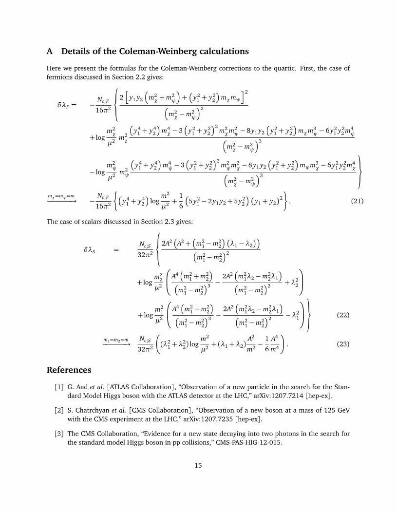
A Details of the Coleman-Weinberg calculations
Here we present the formulas for the Coleman-Weinberg corrections to the quartic. First, the case offermions discussed in Section 2.2 gives:
δλF = −Nc;F
16π2
2h
y1 y2
�
m2χ +m2
ψ
�
+�
y21 + y2
2
�
mχmψi2
�
m2χ −m2
ψ
�2
+ logm2χ
µ2 m2χ
�
y41 + y4
2
�
m4χ − 3
�
y21 + y2
2
�2m2χm2
ψ− 8y1 y2
�
y21 + y2
2
�
mχm3ψ− 6y2
1 y22 m4
ψ�
m2χ −m2
ψ
�3
− logm2ψ
µ2 m2ψ
�
y41 + y4
2
�
m4ψ− 3�
y21 + y2
2
�2m2ψm2
χ − 8y1 y2
�
y21 + y2
2
�
mψm3χ − 6y2
1 y22 m4
χ�
m2χ −m2
ψ
�3
mχ=mψ=m−−−−−−→ −
Nc;F
16π2
¨
�
y41 + y4
2
�
logm2
µ2 +1
6
�
5y21 − 2y1 y2+ 5y2
2
�
�
y1+ y2�2
«
. (21)
The case of scalars discussed in Section 2.3 gives:
δλS =Nc;S
32π2
2A2�
A2+�
m21−m2
2
�
�
λ1−λ2�
�
�
m21−m2
2
�2
+ logm2
2
µ2
A4�
m21+m2
2
�
�
m21−m2
2
�3 −2A2�
m21λ2−m2
2λ1
�
�
m21−m2
2
�2 +λ22
+ logm2
1
µ2
A4�
m21+m2
2
�
�
m21−m2
2
�3 −2A2�
m21λ2−m2
2λ1
�
�
m21−m2
2
�2 −λ21
(22)
m1=m2=m−−−−−−→
Nc;S
32π2
�
(λ21+λ
22) log
m2
µ2 + (λ1+λ2)A2
m2 −1
6
A4
m4
�
. (23)
References
[1] G. Aad et al. [ATLAS Collaboration], “Observation of a new particle in the search for the Stan-dard Model Higgs boson with the ATLAS detector at the LHC,” arXiv:1207.7214 [hep-ex].
[2] S. Chatrchyan et al. [CMS Collaboration], “Observation of a new boson at a mass of 125 GeVwith the CMS experiment at the LHC,” arXiv:1207.7235 [hep-ex].
[3] The CMS Collaboration, “Evidence for a new state decaying into two photons in the search forthe standard model Higgs boson in pp collisions,” CMS-PAS-HIG-12-015.
15
[4] The ATLAS Collaboration, “Observation of an excess of events in the search for the StandardModel Higgs boson in the gamma-gamma channel with the ATLAS detector,” ATLAS-CONF-2012-091.
[5] C. Englert, T. Plehn, M. Rauch, D. Zerwas and P. M. Zerwas, “LHC: Standard Higgs and HiddenHiggs,” Phys. Lett. B 707, 512 (2012) arXiv:1112.3007 [hep-ph].
[6] D. Carmi, A. Falkowski, E. Kuflik and T. Volansky, “Interpreting LHC Higgs Results from NaturalNew Physics Perspective,” arXiv:1202.3144 [hep-ph].
[7] A. Azatov, R. Contino and J. Galloway, “Model-Independent Bounds on a Light Higgs,” JHEP1204, 127 (2012) arXiv:1202.3415 [hep-ph].
[8] J. R. Espinosa, C. Grojean, M. Muhlleitner and M. Trott, “Fingerprinting Higgs Suspects at theLHC,” JHEP 1205, 097 (2012) arXiv:1202.3697 [hep-ph].
[9] P. P. Giardino, K. Kannike, M. Raidal and A. Strumia, “Reconstructing Higgs boson propertiesfrom the LHC and Tevatron data,” JHEP 1206, 117 (2012) arXiv:1203.4254 [hep-ph].
[10] T. Li, X. Wan, Y.-K. Wang and S.-H. Zhu, “Constraints on the Universal Varying Yukawa Couplings:from SM-like to Fermiophobic,” arXiv:1203.5083 [hep-ph].
[11] M. Rauch, “Determination of Higgs-boson couplings (SFitter),” arXiv:1203.6826 [hep-ph].
[12] J. Ellis and T. You, “Global Analysis of Experimental Constraints on a Possible Higgs-Like Particlewith Mass 125 GeV,” JHEP 1206, 140 (2012) arXiv:1204.0464 [hep-ph].
[13] M. Klute, R. Lafaye, T. Plehn, M. Rauch and D. Zerwas, “Measuring Higgs Couplings from LHCData,” Phys. Rev. Lett. 109, 101801 (2012) arXiv:1205.2699 [hep-ph].
[14] A. Azatov, S. Chang, N. Craig and J. Galloway, “Early Higgs Hints for Non-Minimal Supersym-metry,” arXiv:1206.1058 [hep-ph].
[15] D. Carmi, A. Falkowski, E. Kuflik and T. Volansky, “Interpreting the Higgs,” arXiv:1206.4201[hep-ph].
[16] T. Corbett, O. J. P. Eboli, J. Gonzalez-Fraile and M. C. Gonzalez-Garcia, “Constraining anomalousHiggs interactions,” arXiv:1207.1344 [hep-ph].
[17] P. P. Giardino, K. Kannike, M. Raidal and A. Strumia, “Is the resonance at 125 GeV the Higgsboson?,” arXiv:1207.1347 [hep-ph].
[18] M. R. Buckley and D. Hooper, “Are There Hints of Light Stops in Recent Higgs Search Results?,”arXiv:1207.1445 [hep-ph].
[19] J. Ellis and T. You, “Global Analysis of the Higgs Candidate with Mass ∼ 125 GeV,”arXiv:1207.1693 [hep-ph].
[20] M. Montull and F. Riva, “Higgs discovery: the beginning or the end of natural EWSB?,”arXiv:1207.1716 [hep-ph].
16
[21] J. R. Espinosa, C. Grojean, M. Muhlleitner and M. Trott, “First Glimpses at Higgs’ face,”arXiv:1207.1717 [hep-ph].
[22] D. Carmi, A. Falkowski, E. Kuflik, T. Volansky and J. Zupan, “Higgs After the Discovery: A StatusReport,” arXiv:1207.1718 [hep-ph].
[23] T. Plehn and M. Rauch, “Higgs Couplings after the Discovery,” arXiv:1207.6108 [hep-ph].
[24] J. R. Espinosa, C. Grojean, V. Sanz and M. Trott, “NSUSY fits,” arXiv:1207.7355 [hep-ph].
[25] The ATLAS Collaboration, “Observation of an excess of events in the search for the StandardModel Higgs boson in the H → Z Z (∗) → 4` channel with the ATLAS detector,” ATLAS-CONF-2012-092.
[26] The CMS Collaboration, “Evidence for a new state in the search for the standard model Higgsboson in the H to ZZ to 4 leptons channel in pp collisions at sqrt(s) = 7 and 8 TeV,” CMS-PAS-HIG-12-016.
[27] The CMS Collaboration, “Search for the standard model Higgs boson decaying to a W pair in thefully leptonic final state in pp collisions at sqrt(s) = 8 TeV,” CMS-PAS-HIG-12-017.
[28] The ATLAS Collaboration, “Observation of an Excess of Events in the Search for the StandardModel Higgs Boson in the H → WW (∗) → `ν`ν Channel with the ATLAS Detector,” ATLAS-CONF-2012-098.
[29] S. Dimopoulos and G. F. Giudice, “Naturalness constraints in supersymmetric theories withnonuniversal soft terms,” Phys. Lett. B 357, 573 (1995) hep-ph/9507282.
[30] A. G. Cohen, D. B. Kaplan and A. E. Nelson, “The More minimal supersymmetric standardmodel,” Phys. Lett. B 388, 588 (1996) hep-ph/9607394.
[31] J. R. Ellis, M. K. Gaillard and D. V. Nanopoulos, “A Phenomenological Profile of the Higgs Boson,”Nucl. Phys. B 106, 292 (1976).
[32] M. A. Shifman, A. I. Vainshtein, M. B. Voloshin and V. I. Zakharov, “Low-Energy Theorems forHiggs Boson Couplings to Photons,” Sov. J. Nucl. Phys. 30, 711 (1979) [Yad. Fiz. 30, 1368(1979)].
[33] A. G. Cohen and M. Schmaltz, “New Charged Particles from Higgs Couplings,” arXiv:1207.3495[hep-ph].
[34] I. Dorsner, S. Fajfer, A. Greljo, and J. F. Kamenik, “Higgs Uncovering Light Scalar Remnants ofHigh Scale Matter Unification,” arXiv:1208.1266 [hep-ph].
[35] S. P. Martin, “A Supersymmetry primer,” In Kane, G.L. (ed.): Perspectives on supersymmetry II1-153 hep-ph/9709356.
[36] M. S. Carena, M. Quiros and C. E. M. Wagner, “Effective potential methods and the Higgs massspectrum in the MSSM,” Nucl. Phys. B 461, 407 (1996) hep-ph/9508343.
[37] N. Arkani-Hamed, K. Blum, R. T. D’Agnolo and J. Fan, “2:1 for Naturalness at the LHC?,”arXiv:1207.4482 [hep-ph].
17
[38] A. Kusenko, P. Langacker and G. Segre, “Phase transitions and vacuum tunneling into chargeand color breaking minima in the MSSM,” Phys. Rev. D 54, 5824 (1996) hep-ph/9602414.
[39] K. Blum, R. T. D’Agnolo and J. Fan, “Natural SUSY Predicts: Higgs Couplings,” arXiv:1206.5303[hep-ph].
[40] The ATLAS Collaboration, “Search for light top squark pair production in final states with leptonsand b-jets with the ATLAS detector in
ps = 7 TeV proton–proton collisions,” ATLAS-CONF-2012-
070.
[41] The ATLAS Collaboration, “Search for light top squark pair production in final states with leptonsand b-jets with the ATLAS detector in
ps = 7 TeV proton–proton collisions,” ATLAS-CONF-2012-
071.
[42] The ATLAS Collaboration, “Search for direct top squark pair production in final states with oneisolated lepton, jets, and missing transverse momentum in
ps = 7 TeV pp collisions using 4.7
fb−1 of ATLAS data ,” ATLAS-CONF-2012-073.
[43] The ATLAS Collaboration, “Search for a supersymmetric partner of the top quark in final stateswith jets and missing transverse momentum at
ps=7 TeV with the ATLAS detector ,” ATLAS-
CONF-2012-074.
[44] The CMS Collaboration, “A search for the decays of a new heavy particle in multijet events withthe razor variables at CMS in pp collisions at
ps=7 TeV,” CMS-PAS-SUS-12-009.
[45] The CMS Collaboration, “Search for supersymmetery in final states with missing transverse mo-mentum and 0, 1, 2, or ≥ 3 b jets with CMS,” CMS-PAS-SUS-11-022.
[46] P. Meade and M. Reece, “Top partners at the LHC: Spin and mass measurement,” Phys. Rev. D74, 015010 (2006) hep-ph/0601124.
[47] T. Han, R. Mahbubani, D. G. E. Walker and L. -T. Wang, “Top Quark Pair plus Large MissingEnergy at the LHC,” JHEP 0905, 117 (2009) arXiv:0803.3820 [hep-ph].
[48] T. Plehn, M. Spannowsky, M. Takeuchi and D. Zerwas, “Stop Reconstruction with Tagged Tops,”JHEP 1010, 078 (2010) arXiv:1006.2833 [hep-ph].
[49] M. Asano, H. D. Kim, R. Kitano and Y. Shimizu, “Natural Supersymmetry at the LHC,” JHEP1012, 019 (2010) arXiv:1010.0692 [hep-ph].
[50] T. Plehn, M. Spannowsky and M. Takeuchi, “Boosted Semileptonic Tops in Stop Decays,” JHEP1105, 135 (2011) arXiv:1102.0557 [hep-ph].
[51] Y. Bai, H. -C. Cheng, J. Gallicchio and J. Gu, “Stop the Top Background of the Stop Search,”JHEP 1207, 110 (2012) arXiv:1203.4813 [hep-ph].
[52] T. Plehn, M. Spannowsky and M. Takeuchi, “Stop searches in 2012,” arXiv:1205.2696 [hep-ph].
[53] D. S. M. Alves, M. R. Buckley, P. J. Fox, J. D. Lykken and C. -T. Yu, “Stops and MET: the shape ofthings to come,” arXiv:1205.5805 [hep-ph].
18
[54] D. E. Kaplan, K. Rehermann and D. Stolarski, “Searching for Direct Stop Production in HadronicTop Data at the LHC,” JHEP 1207, 119 (2012) arXiv:1205.5816 [hep-ph].
[55] C. -Y. Chen, A. Freitas, T. Han and K. S. M. Lee, “New Physics from the Top at the LHC,”arXiv:1207.4794 [hep-ph].
[56] Z. Han, A. Katz, D. Krohn and M. Reece, “(Light) Stop Signs,” to appear in JHEP, arXiv:1205.5808[hep-ph].
[57] C. Brust, A. Katz and R. Sundrum, “SUSY Stops at a Bump,” arXiv:1206.2353 [hep-ph].
[58] C. L. Wainwright, “CosmoTransitions: Computing Cosmological Phase Transi-tion Temperatures and Bubble Profiles with Multiple Fields,” Comput. Phys. Com-mun. 183, 2006 (2012) arXiv:1109.4189 [hep-ph]; Software version 1.0.1 fromhttp://chasm.ucsc.edu/cosmotransitions/.
[59] G. Abbiendi et al. [OPAL Collaboration], “Search for scalar top and scalar bottom quarks at LEP,”Phys. Lett. B 545, 272 (2002) [Erratum-ibid. B 548, 258 (2002)] hep-ex/0209026.
[60] P. Achard et al. [L3 Collaboration], “Search for scalar leptons and scalar quarks at LEP,” Phys.Lett. B 580, 37 (2004) hep-ex/0310007.
[61] A. V. Manohar and M. B. Wise, “Flavor changing neutral currents, an extended scalar sector, andthe Higgs production rate at the CERN LHC,” Phys. Rev. D 74, 035009 (2006) hep-ph/0606172.
[62] Y. Bai, J. Fan and J. L. Hewett, “Hiding a Heavy Higgs Boson at the 7 TeV LHC,” arXiv:1112.1964[hep-ph].
[63] B. A. Dobrescu, G. D. Kribs and A. Martin, “Higgs Underproduction at the LHC,” Phys. Rev. D85, 074031 (2012) arXiv:1112.2208 [hep-ph].
[64] K. Kumar, R. Vega-Morales and F. Yu, “Effects from New Colored States and the Higgs Portal onGluon Fusion and Higgs Decays,” arXiv:1205.4244 [hep-ph].
[65] B. Batell, S. Gori and L. -T. Wang, “Exploring the Higgs Portal with 10/fb at the LHC,” JHEP1206, 172 (2012) arXiv:1112.5180 [hep-ph].
[66] G. D. Kribs and A. Martin, “Enhanced di-Higgs Production through Light Colored Scalars,”arXiv:1207.4496 [hep-ph].
[67] G. Aad et al. [ATLAS Collaboration], “Search for Massive Colored Scalars in Four-Jet Final Statesin sqrts=7 TeV proton-proton collisions with the ATLAS Detector,” Eur. Phys. J. C 71, 1828(2011) arXiv:1110.2693 [hep-ex].
[68] The CMS Collaboration, “Search for New Physics in the Paired Dijet Mass Spectrum,” CMS-PAS-EXO-11-016.
[69] C. P. Burgess, M. Trott and S. Zuberi, “Light Octet Scalars, a Heavy Higgs and Minimal FlavourViolation,” JHEP 0909, 082 (2009) arXiv:0907.2696 [hep-ph].
[70] W. Altmannshofer, R. Primulando, C. -T. Yu and F. Yu, “New Physics Models of Direct CP Violationin Charm Decays,” JHEP 1204, 049 (2012) arXiv:1202.2866 [hep-ph].
19
[71] M. Carena, S. Gori, N. R. Shah and C. E. M. Wagner, “A 125 GeV SM-like Higgs in the MSSM andthe γγ rate,” JHEP 1203, 014 (2012) arXiv:1112.3336 [hep-ph].
[72] M. Carena, S. Gori, N. R. Shah, C. E. M. Wagner and L. -T. Wang, “Light Stau Phenomenologyand the Higgs γγ Rate,” arXiv:1205.5842 [hep-ph].
[73] M. Carena, I. Low and C. E. M. Wagner, “Implications of a Modified Higgs to Diphoton DecayWidth,” arXiv:1206.1082 [hep-ph].
[74] A. Joglekar, P. Schwaller and C. E. M. Wagner, “Dark Matter and Enhanced Higgs to Di-photonRate from Vector-like Leptons,” arXiv:1207.4235 [hep-ph].
[75] H. An, T. Liu and L. -T. Wang, “125 GeV Higgs Boson, Enhanced Di-photon Rate, and GaugedU(1)PQ-Extended MSSM,” arXiv:1207.2473 [hep-ph].
[76] L. G. Almeida, E. Bertuzzo, P. A. N. Machado and R. Z. Funchal, “Does H → γγ Taste like vanillaNew Physics?,” arXiv:1207.5254 [hep-ph].
[77] A. Alves, E. Ramirez Barreto, A. G. Dias, C. A. de S.Pires, F. S. Queiroz and P. S. Rodrigues daSilva, “Probing 3-3-1 Models in Diphoton Higgs Boson Decay,” Phys. Rev. D 84, 115004 (2011)arXiv:1109.0238 [hep-ph].
[78] A. Alves, A. G. Dias, E. R. Barreto, C. A. d. S. Pires, F. S. Queiroz and P. S. R. da Silva, “Explainingthe Higgs Decays at the LHC with an Extended Electroweak Model,” arXiv:1207.3699 [hep-ph].
[79] L. J. Hall, D. Pinner and J. T. Ruderman, “A Natural SUSY Higgs Near 126 GeV,” JHEP 1204, 131(2012) arXiv:1112.2703 [hep-ph].
[80] K. Blum and R. T. D’Agnolo, “2 Higgs or not 2 Higgs,” Phys. Lett. B 714, 66 (2012)arXiv:1202.2364 [hep-ph].
[81] K. Hagiwara, J. S. Lee and J. Nakamura, “Properties of 125 GeV Higgs boson in non-decouplingMSSM scenarios,” arXiv:1207.0802 [hep-ph].
[82] B. Bellazzini, C. Petersson and R. Torre, “Photophilic Higgs from sgoldstino mixing,” Phys. Rev.D 86, 033016 (2012) arXiv:1207.0803 [hep-ph].
[83] N. Craig and S. Thomas, “Exclusive Signals of an Extended Higgs Sector,” arXiv:1207.4835 [hep-ph].
[84] D. S. M. Alves, P. J. Fox and N. J. Weiner, “Higgs Signals in a Type I 2HDM or with a Sister Higgs,”arXiv:1207.5499 [hep-ph].
20