Use of Computer Technology for Insight and Proof A. Eight Historical Examples B. Weaknesses and...
50
Use of Computer Technology for Insight and Proof A. Eight Historical Examples B. Weaknesses and Strengths R. Wilson Barnard, Kent Pearce Texas Tech University Presentation: January 2010
-
Upload
reynard-day -
Category
Documents
-
view
213 -
download
0
Transcript of Use of Computer Technology for Insight and Proof A. Eight Historical Examples B. Weaknesses and...

Use of Computer Technology for Insight and Proof
A. Eight Historical ExamplesB. Weaknesses and Strengths
R. Wilson Barnard, Kent Pearce
Texas Tech University
Presentation: January 2010
Eight Historical Examples
π/4’s Conjecture 2/3’s Conjecture Omitted Area Problem Polynomials with Nonnegative Coefficients
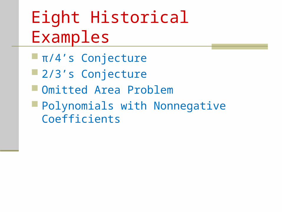
Eight Historical Examples
π/4’s Conjecture 2/3’s Conjecture Omitted Area Problem Polynomials with Nonnegative Coefficients Coefficient Conjecture of Brannan Bounds for Schwarzian Derivatives for
Hyperbolically Convex Functions Iceberg-type Problems in Two-Dimensions Campbell’s Subordination Conjecture
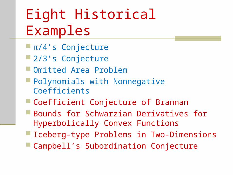
π/4’s Conjecture
Let D denote the open unit disk in the complex plane and let A be the set of analytical functions on D.
Let S denote the usual subset of A of normalized univalent functions.
Let L denote a continuous linear functional on A. A support point of S (with respect to L) is a
function such thatf S
Re ( ) Re ( ) for allL f L g g S
π/4’s Conjecture
In ’70s, one of the active approaches to attacking the Bieberbach Conjecture was routed through an investigation of extreme points and support points of S (since coefficient functionals are among other things linear).
Brickman, Brown, Duren, Hengartner, Kirwan, Leung, MacGregor, Pell, Pfluger, Ruscheweyh, Schaeffer, Schiffer, Schober, Spencer, Wilken
π/4’s Conjecture
Using boundary variational techniques, certain necessary conditions were deduced that a support point of S had to satisfy. Specifically, if Γ is the complement of the range of a support point of S, then Γ is a trajectory of a quadratic differential Γ is a single analytical arc tending to ∞ Γ tends to ∞ with monotonically increasing modulus Γ is asymptotic to a half-line at ∞ Γ satisfies the “π/4 property”
π/4’s Conjecture
π/4’s Conjecture
π/4’s Conjecture
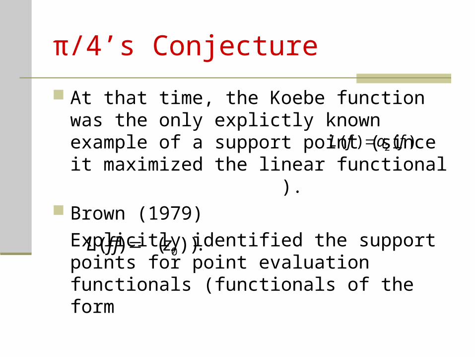
At that time, the Koebe function was the only explictly known example of a support point (since it maximized the linear functional ).
Brown (1979)
Explicitly identified the support points for point evaluation functionals (functionals of the form
2( ) ( )L f a f
0( ) ( ) ).L f f z
π/4’s Conjecture
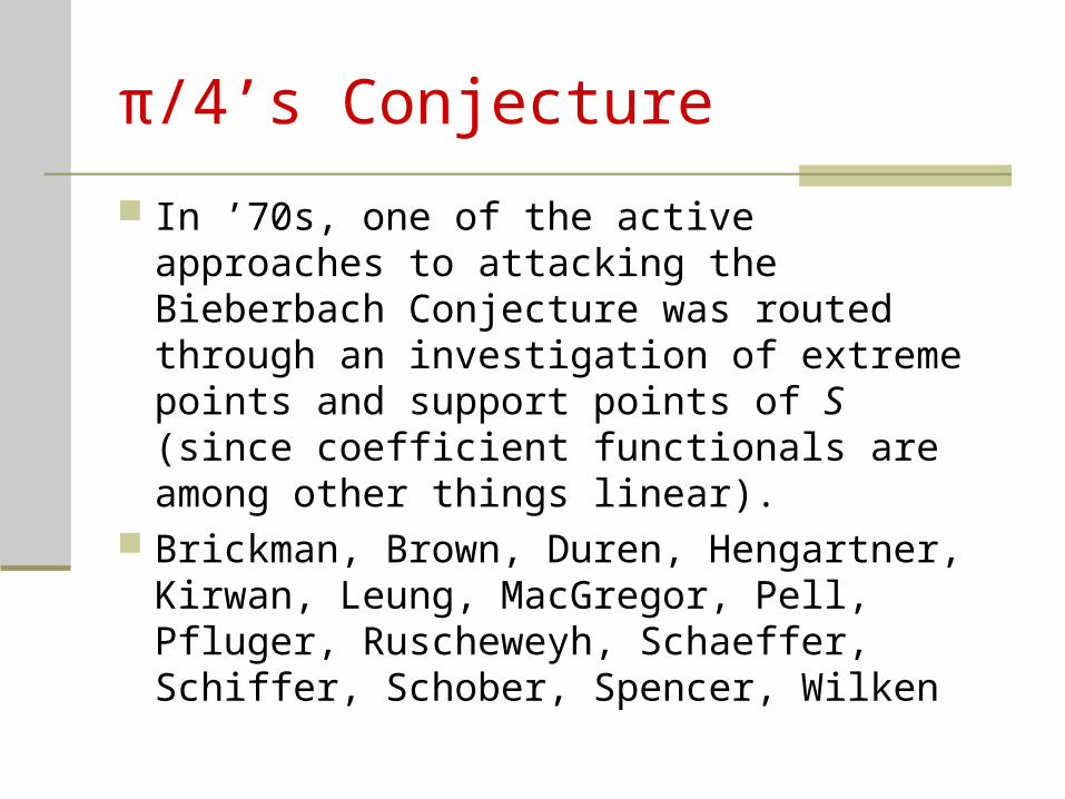
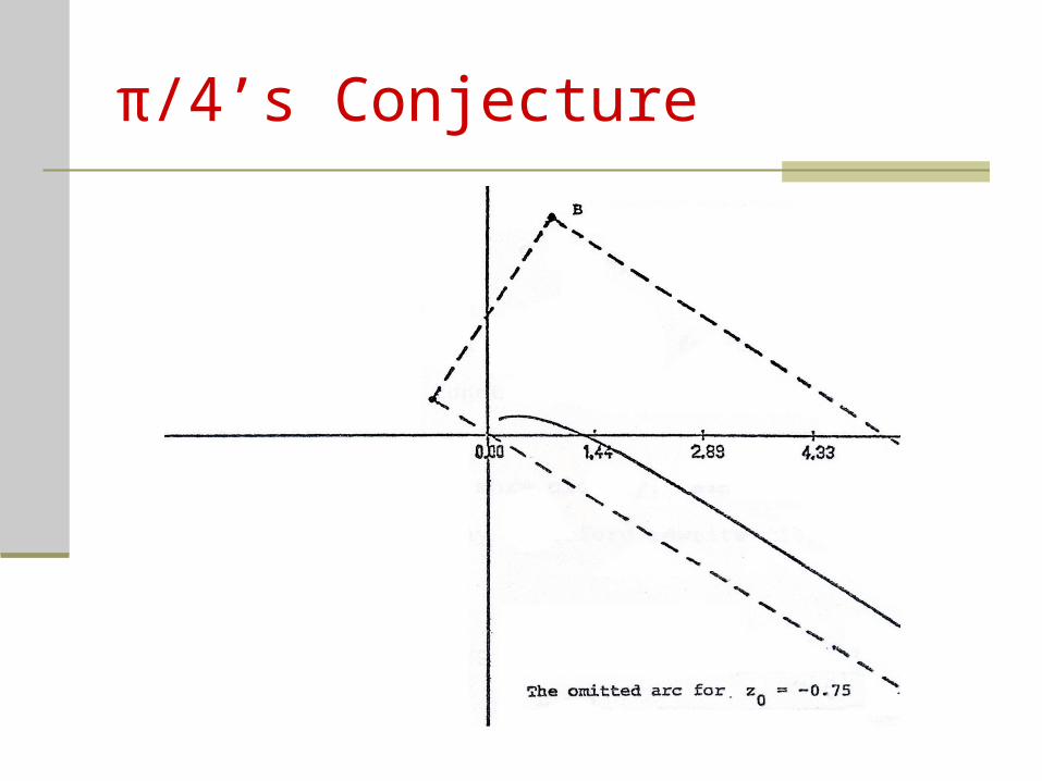
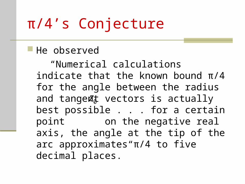
He observed
“Numerical calculations indicate that the known bound π/4 for the angle between the radius and tangent vectors is actually best possible . . . for a certain point on the negative real axis, the angle at the tip of the arc approximates π/4 to five decimal places.”
0z
π/4’s Conjecture
Shortly thereafter, I made an observation that a sharp result of Goluzin for bounding the argument of the derivative of a function in S could be interpreted to identify certain associated extremal functions (close-to-convex half-line mappings) as a support points of S and that π/4 was achieved exactly at the finite tip of the omitted half-line for two of these half-line mappings.
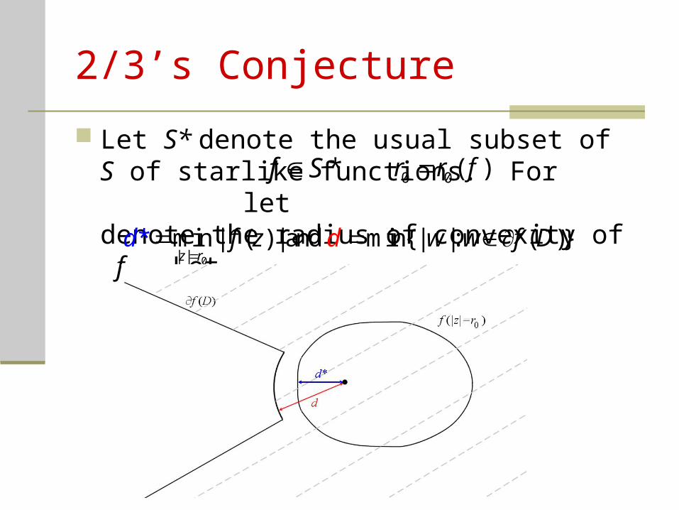
2/3’s Conjecture
Let S* denote the usual subset of S of starlike functions. For let denote the radius of convexity of f. Let
*f S 0 0 ( )r r f
0| |min | ( ) | and min{| |: ( )}*z r
f z w w f Ddd
2/3’s Conjecture
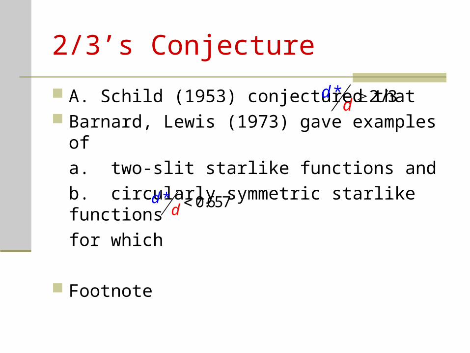
A. Schild (1953) conjectured that Barnard, Lewis (1973) gave examples of
a. two-slit starlike functions and
b. circularly symmetric starlike functions
for which
Footnote
2* / 3dd
0* .657dd
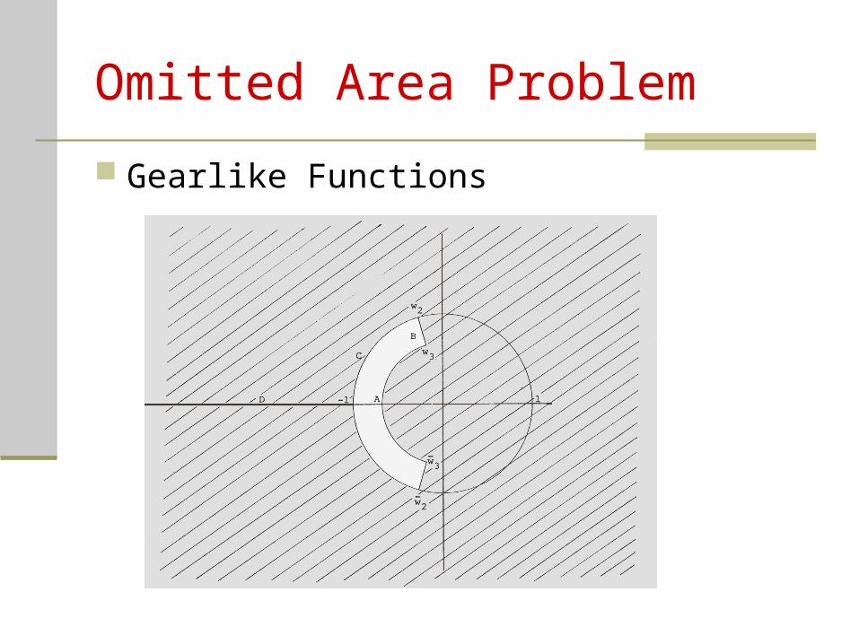
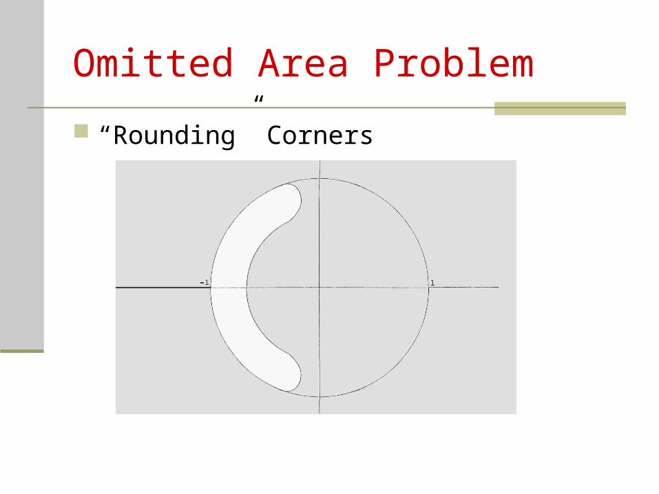
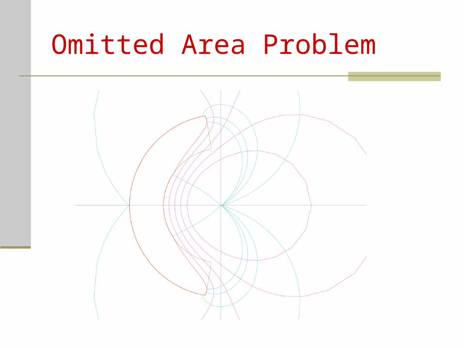
Omitted Area Problem
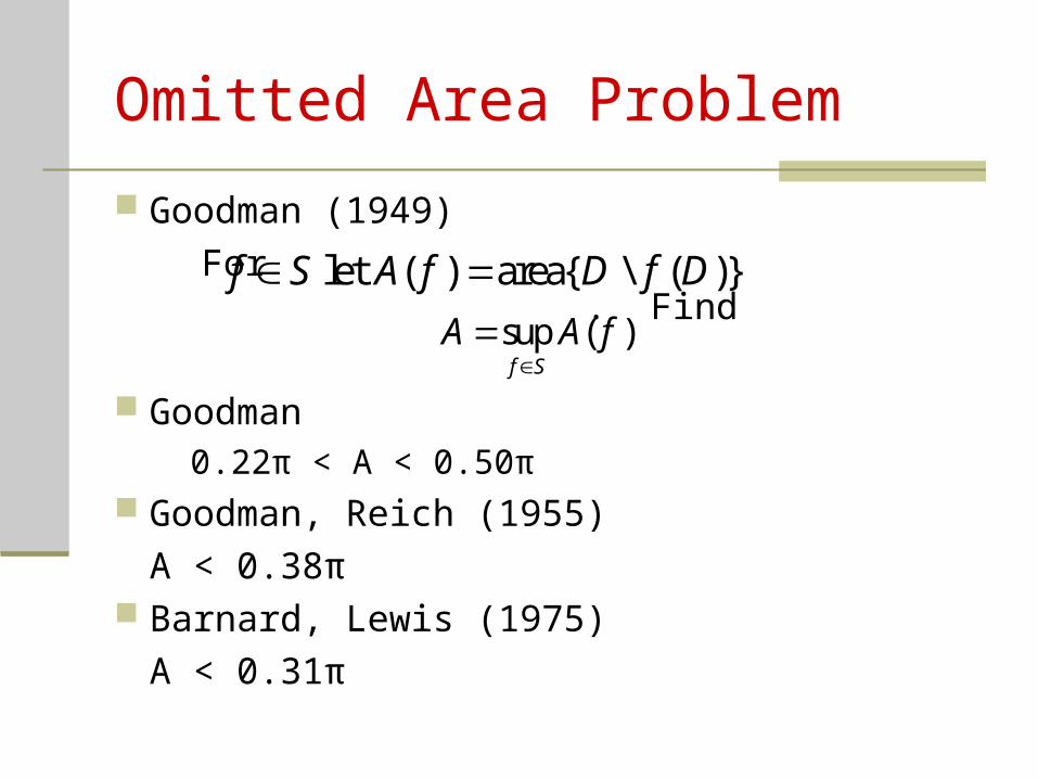
Goodman (1949)
For . Find
Goodman
0.22π < A < 0.50π Goodman, Reich (1955)
A < 0.38π Barnard, Lewis (1975)
A < 0.31π
let ( ) area{ \ ( )}f S A f D f D sup ( )f S
A A f
Omitted Area Problem
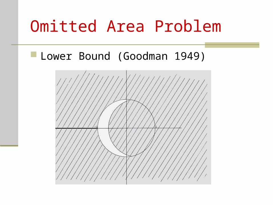
Lower Bound (Goodman 1949)
Omitted Area Problem
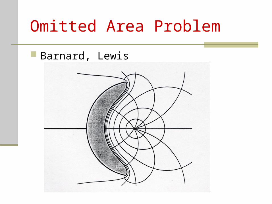
Barnard, Lewis
Omitted Area Problem
Gearlike Functions
Omitted Area Problem
“Rounding” Corners
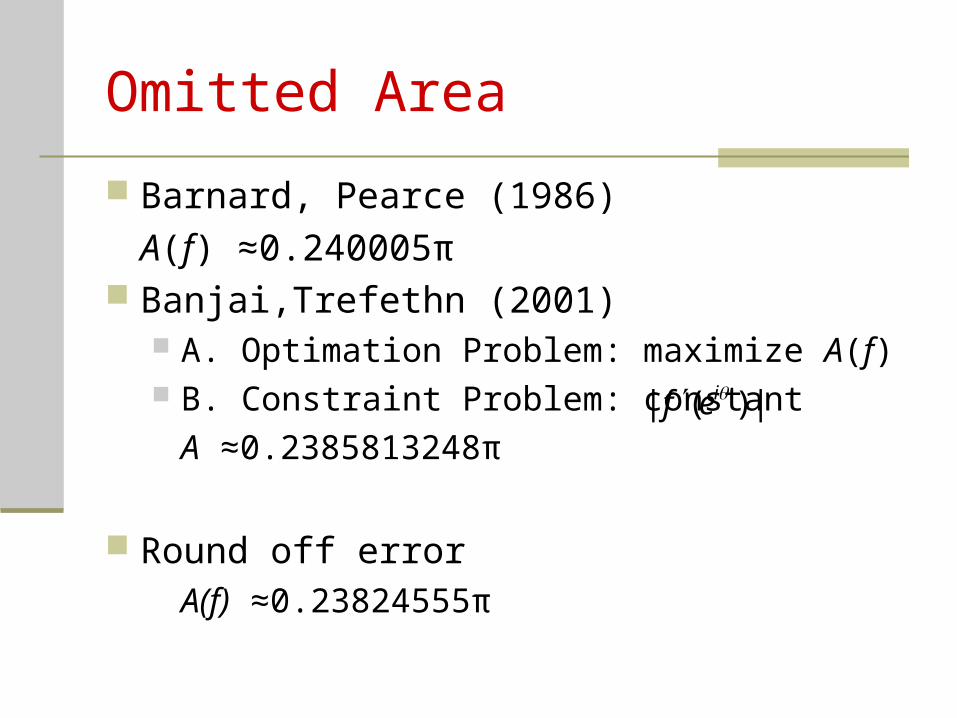
Omitted Area
Barnard, Pearce (1986)
A(f) ≈0.240005π Banjai,Trefethn (2001)
A. Optimation Problem: maximize A(f) B. Constraint Problem: constant
A ≈0.2385813248π
Round off errorA(f) ≈0.23824555π
| ( ) |if e
Omitted Area Problem
Polynomials with Nonnegative Coefficients Can a conjugate pair of zeros be factored from a
polynomial with nonnegative coefficients so that the resulting polynomial still has nonnegative roots?
Polynomials with Nonnegative Coefficients Initially, we supposed that if the pair of zeros with
greatest real part were factored out, the result would hold
In fact, it is true for polynomials of degree less than 6
But,
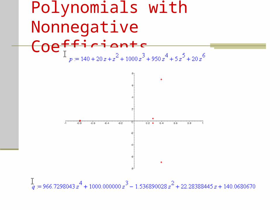
Polynomials with Nonnegative Coefficients
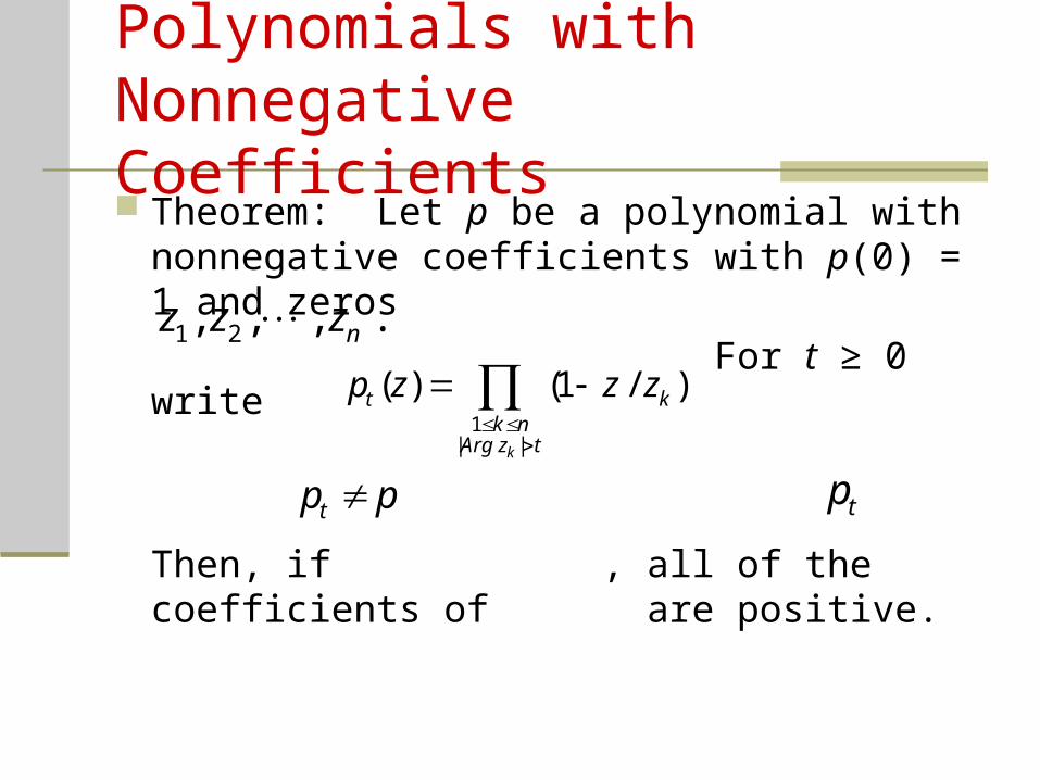
Polynomials with Nonnegative Coefficients Theorem: Let p be a polynomial with nonnegative
coefficients with p(0) = 1 and zeros
For t ≥ 0 write
Then, if , all of the coefficients of are positive.
1 2, , , .nz z z
1| |
( ) (1 / )
k
t kk n
Arg z t
p z z z
tp p tp
Linearity/Monotonicity Arguments
Sturm Sequence Arguments Coefficient Conjecture of Brannan Bounds for Schwarzian Derivatives for
Hyperbolically Convex Functions Iceberg-type Problems in Two-Dimensions Campbell’s Subordination Conjecture
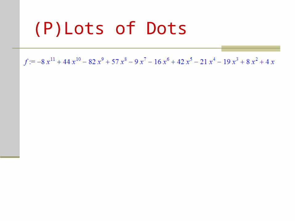
(P)Lots of Dots
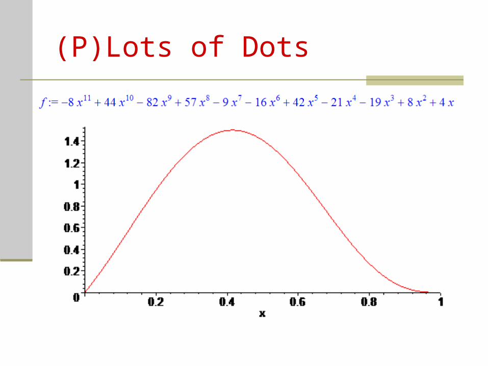
(P)Lots of Dots
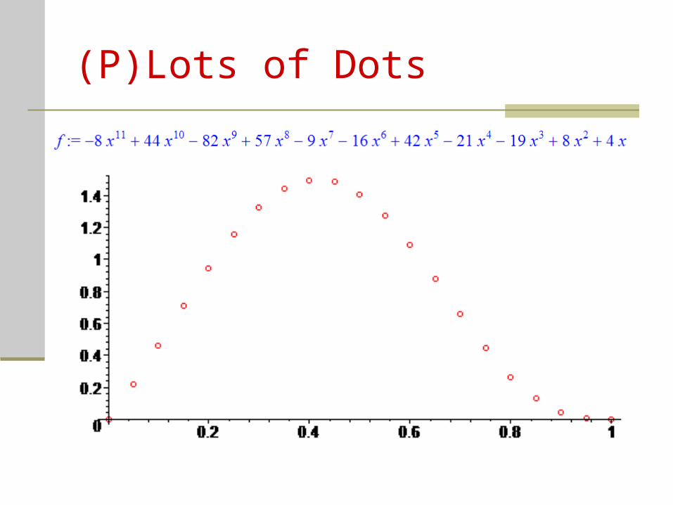
(P)Lots of Dots
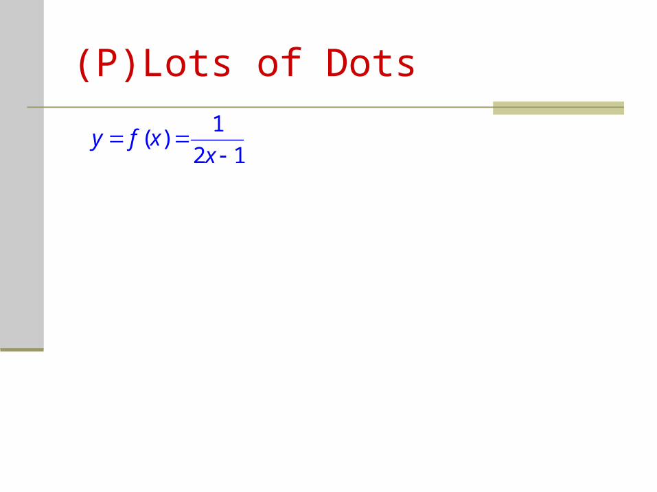
(P)Lots of Dots
1( )
2 1y f x
x
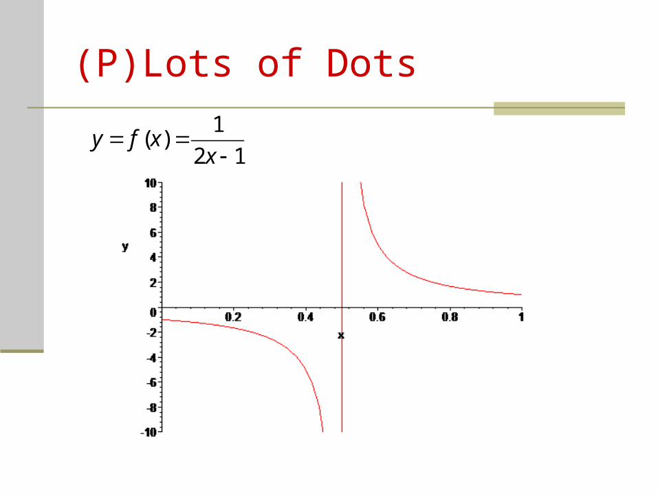
(P)Lots of Dots
1( )
2 1y f x
x
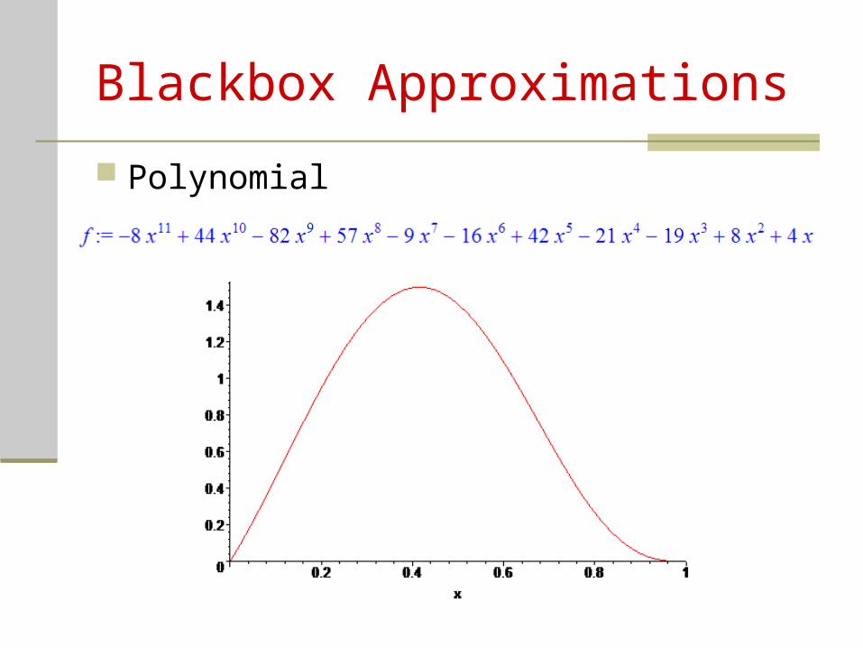
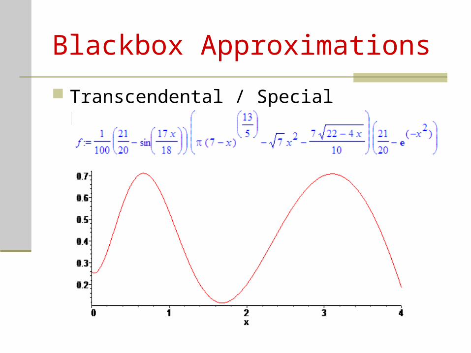
Blackbox Approximations
Polynomial
Blackbox Approximations
Transcendental / Special Functions
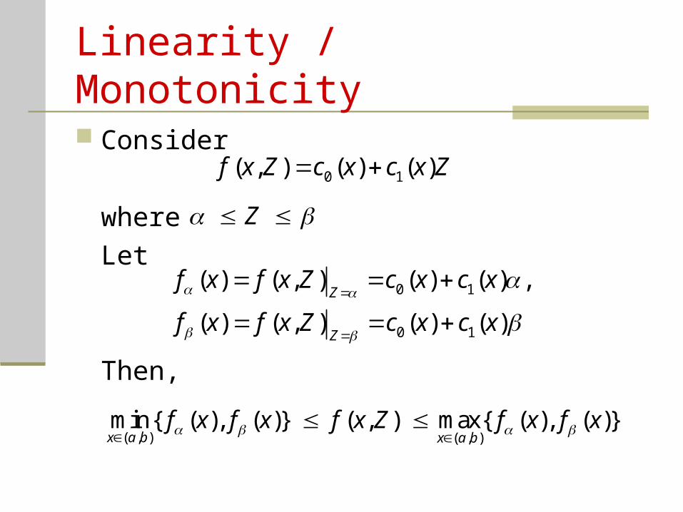
Linearity / Monotonicity
Consider
where
Let
Then,
0 1( , ) ( ) ( )f x Z c x c x Z
Z
0 1
0 1
( ) ( , ) ( ) ( ) ,
( ) ( , ) ( ) ( )Z
Z
f x f x Z c x c x
f x f x Z c x c x
( , ) ( , )min { ( ), ( )} ( , ) max{ ( ), ( )}x a b x a b
f x f x f x Z f x f x
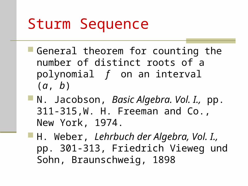
Sturm Sequence
General theorem for counting the number of distinct roots of a polynomial f on an interval (a, b)
N. Jacobson, Basic Algebra. Vol. I., pp. 311-315,W. H. Freeman and Co., New York, 1974.
H. Weber, Lehrbuch der Algebra, Vol. I., pp. 301-313, Friedrich Vieweg und Sohn, Braunschweig, 1898
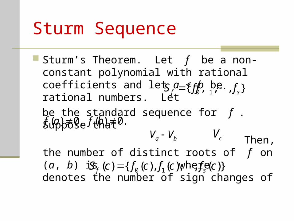
Sturm Sequence
Sturm’s Theorem. Let f be a non-constant polynomial with rational coefficients and let a < b be rational numbers. Let
be the standard sequence for f . Suppose that
Then, the number of distinct roots of f on (a, b) is where denotes the number of sign changes of
0 1{ , , , }f sS f f f
( ) 0, ( ) 0.f a f b a bV V cV
0 1( ) { ( ), ( ), , ( )}f sS c f c f c f c
Sturm Sequence
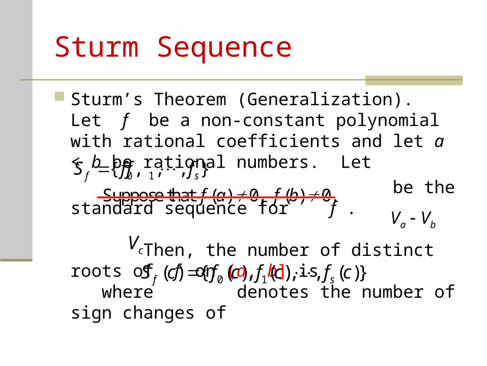
Sturm’s Theorem (Generalization). Let f be a non-constant polynomial with rational coefficients and let a < b be rational numbers. Let
be the standard sequence for f . Then, the number of distinct roots of f on (a, b] is where denotes the number of sign changes of
0 1{ , , , }f sS f f f Suppose that ( ) 0, ( ) 0.f a f b
a bV V
cV
0 1( ) { ( ), ( ), , ( )}f sS c f c f c f c
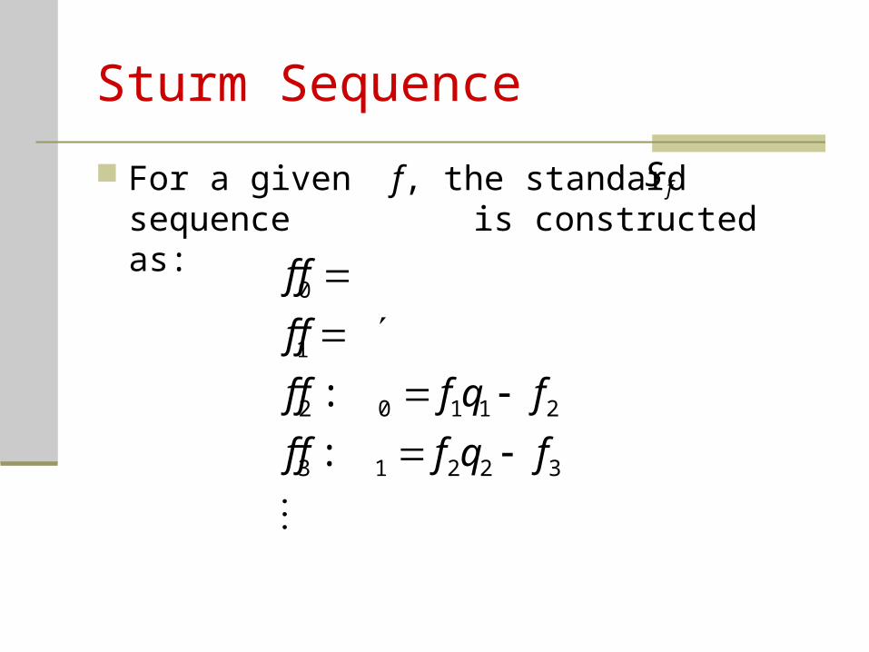
Sturm Sequence
For a given f, the standard sequence is constructed as:
fS
0
1
2 0 1 1 2
3 1 2 2 3
:
:
f f
f f
f f f q f
f f f q f
Sturm Sequence
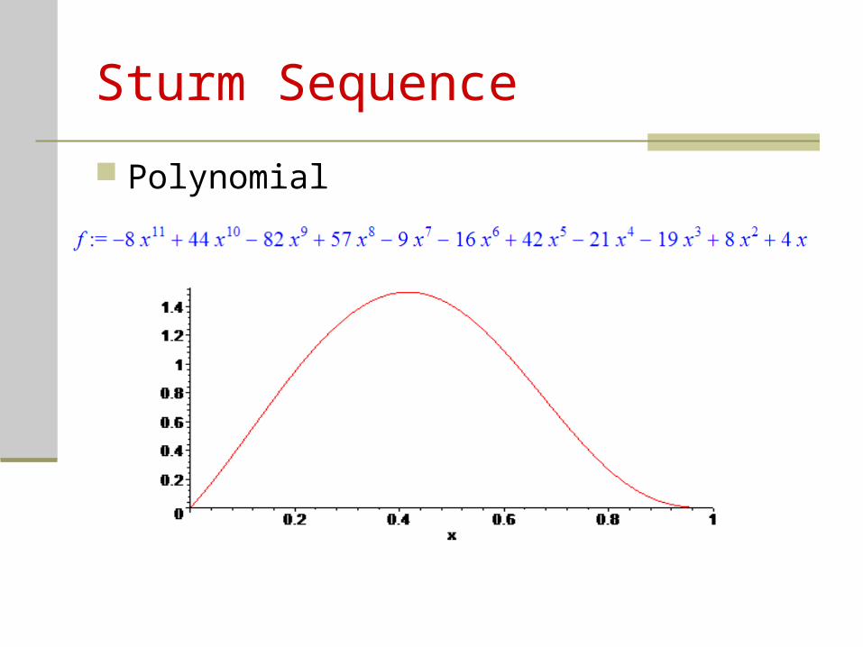
Polynomial
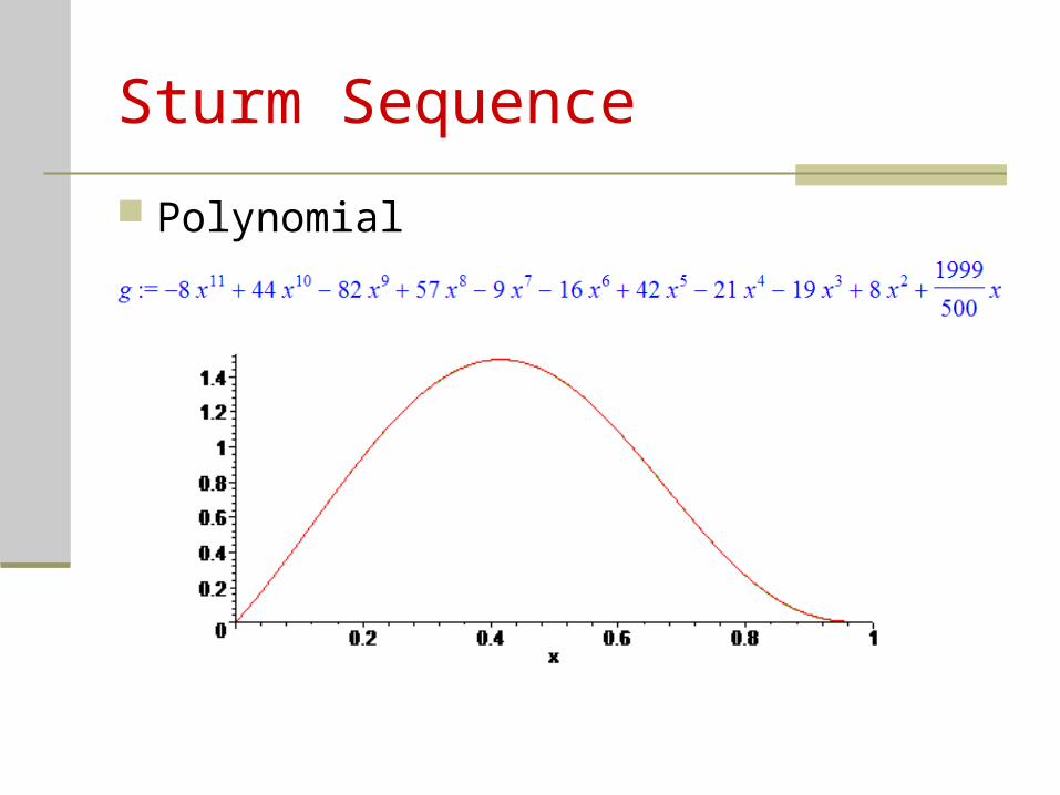
Sturm Sequence
Polynomial
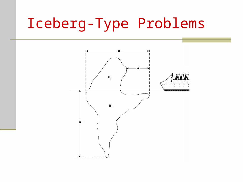
Iceberg-Type Problems
Iceberg-Type Problems
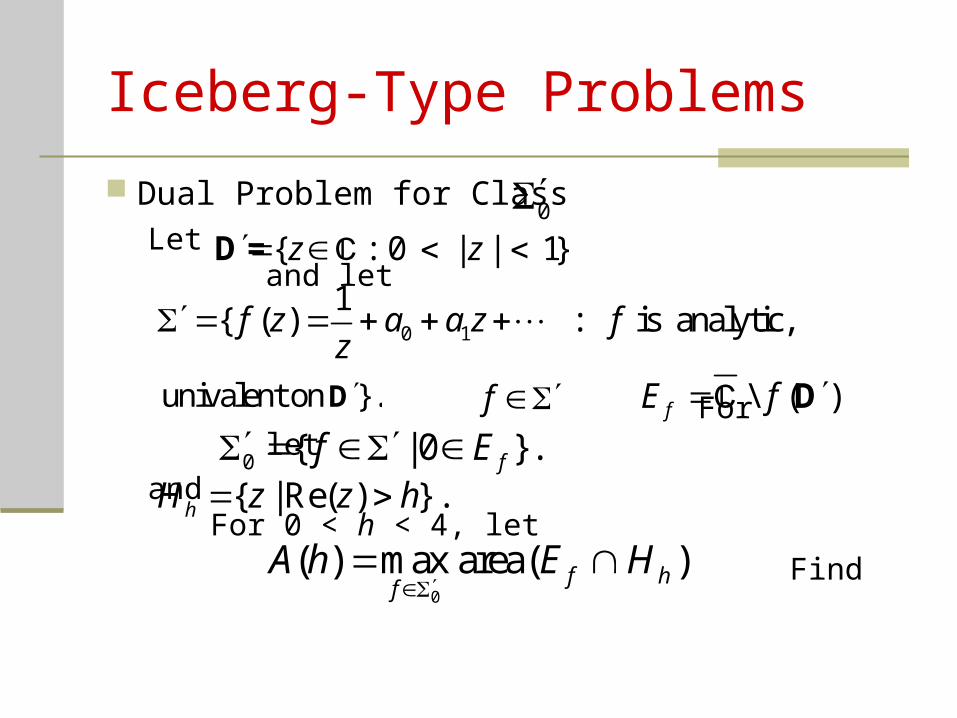
Dual Problem for Class Let and let
For let
and For 0 < h < 4, let
Find
0
( ) max area( )f hf
A h E H
{ | Re( ) }.hH z z h
0
0 1
1{ ( ) : is analytic,f z a a z f
z
univalent on }.D f \ ( )fE f D
0 { | 0 }.ff E
{ : 0 | | 1}z z D=
Iceberg-Type Problems
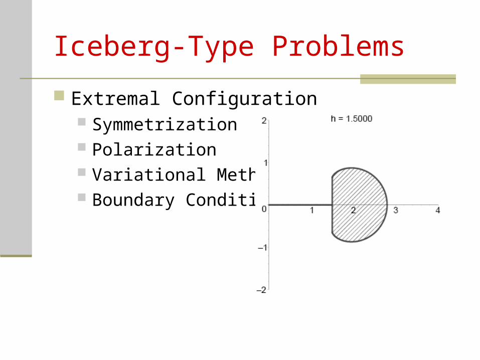
Extremal Configuration Symmetrization Polarization Variational Methods Boundary Conditions
Iceberg-Type Problems
Iceberg-Type Problems
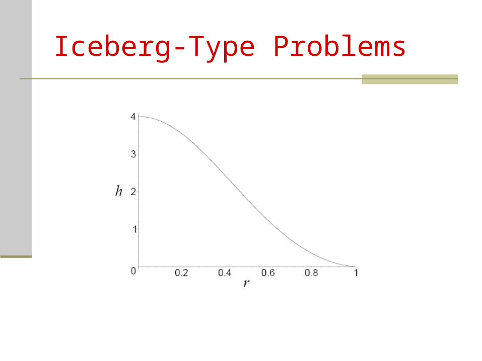
We obtained explicit formulas for A = A(r)
and h = h(r). However, the orginial problem was formulated to find A as a function of h, i.e. to find A = A(h).
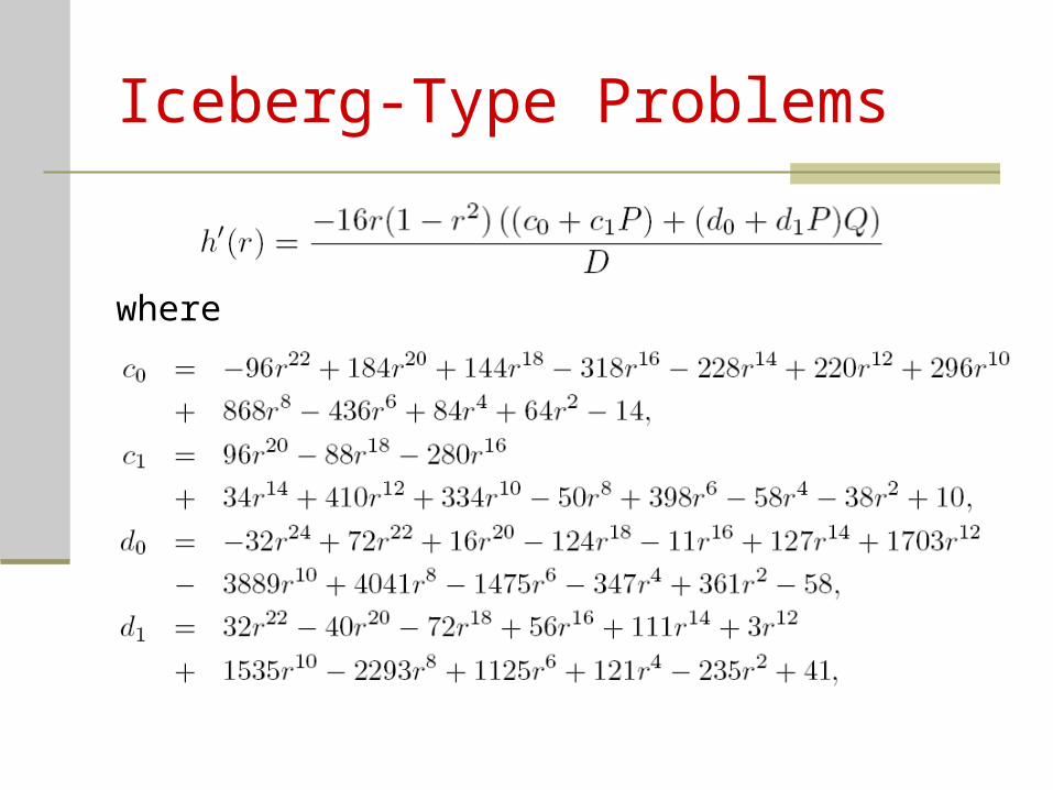
To find an explicit formulation giving A = A(h), we needed to verify that h = h(r) was monotone.
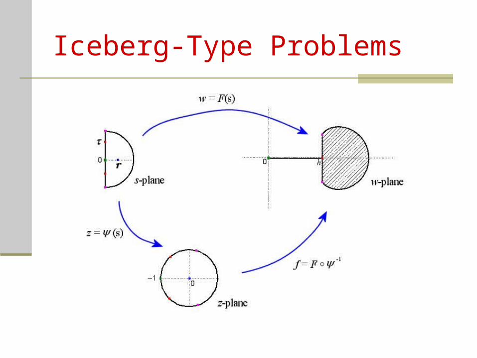
Iceberg-Type Problems
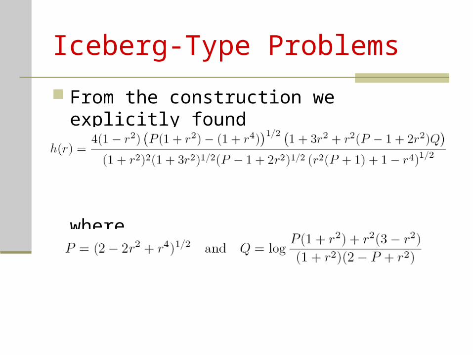
From the construction we explicitly found
where
Iceberg-Type Problems
Iceberg-Type Problems
where
Iceberg-Type Problems
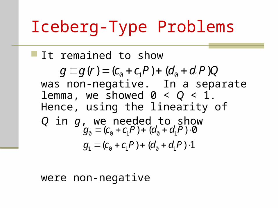
It remained to show
was non-negative. In a separate lemma, we showed 0 < Q < 1. Hence, using the linearity ofQ in g, we needed to show
were non-negative
0 1 0 1( ) ( ) ( )g g r c c P d d P Q
0 0 1 0 1
1 0 1 0 1
( ) ( ) 0
( ) ( ) 1
g c c P d d P
g c c P d d P
Iceberg-Type Problems
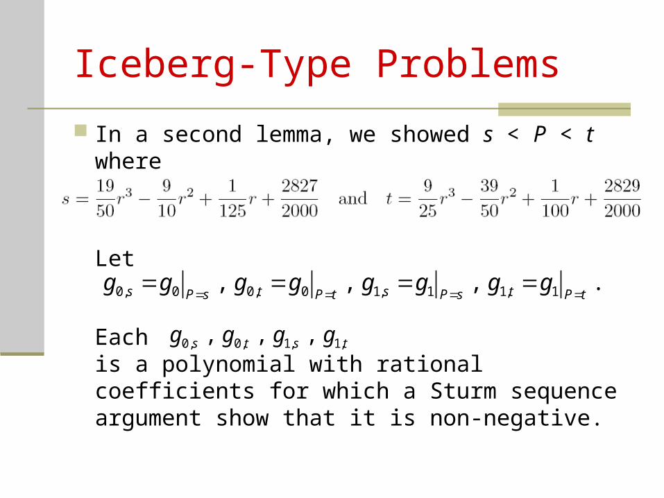
In a second lemma, we showed s < P < t where
Let
Each is a polynomial with rational coefficients for which a Sturm sequence argument show that it is non-negative.
0, 0 0, 0 1, 1 1, 1, , , .s t s tP s P t P s P tg g g g g g g g
0, 0, 1, 1,, , ,s t s tg g g g
Conclusions
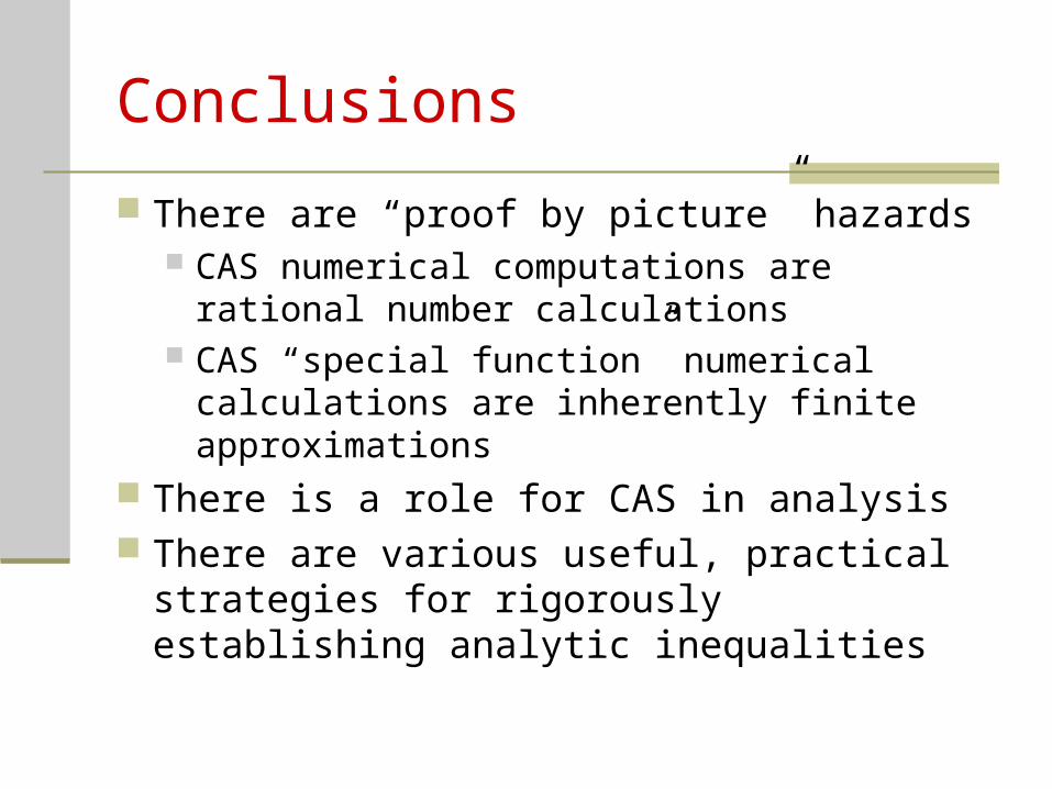
There are “proof by picture” hazards CAS numerical computations are rational number
calculations CAS “special function” numerical calculations are
inherently finite approximations There is a role for CAS in analysis There are various useful, practical strategies for
rigorously establishing analytic inequalities


![A DAY IN MY LIFE Spotlight 4. T HEY GO TO SCHOOL … [eı][ð][aı][α:] eighttheylightclass saytheirwritelarge “They go to school at eight,” Says little Kate.](https://static.fdocument.org/doc/165x107/5a4d1b327f8b9ab05999b779/a-day-in-my-life-spotlight-4-t-hey-go-to-school-eiai.jpg)