arX

iv:0

901.

2526

v1 [

astr

o-ph

.GA

] 16

Jan

200

9

Mon. Not. R. Astron. Soc.000, 1–20 (2008) Printed 1 June 2018 (MN LATEX style file v2.2)

Understanding the H2/HI Ratio in Galaxies

D. Obreschkow and S. RawlingsAstrophysics, Department of Physics, University of Oxford, Keble Road, Oxford, OX1 3RH, UK

Draft 1 June 2018

ABSTRACTWe revisit the mass ratioηgalaxy between molecular hydrogen (H2) and atomic hydrogen (HI)in different galaxies from a phenomenological and theoretical viewpoint. First, the local H2-mass function (MF) is estimated from the local CO-luminosity function (LF) of the FCRAOExtragalactic CO-Survey, adopting a variable CO-to-H2 conversion fitted to nearby observa-tions. This implies an average H2-densityΩH2 = (6.9±2.7)·10−5h−1 andΩH2/ΩHI = 0.26±0.11in the local Universe. Second, we investigate the correlations betweenηgalaxyand global galaxyproperties in a sample of 245 local galaxies. Based on these correlations we introduce fourphenomenological models forηgalaxy, which we apply to estimate H2-masses for each HI-galaxy in the HIPASS catalogue. The resulting H2-MFs (one for each model forηgalaxy) arecompared to the reference H2-MF derived from the CO-LF, thus allowing us to determinethe Bayesian evidence of each model and to identify a clear best model, in which, for spi-ral galaxies,ηgalaxy negatively correlates with both galaxy Hubble type and total gas mass.Third, we derive a theoretical model forηgalaxy for regular galaxies based on an expression fortheir axially symmetric pressure profile dictating the degree of molecularization. This modelis quantitatively similar to the best phenomenological oneat redshiftz = 0, and hence repre-sents a consistent generalization while providing a physical explanation for the dependenceof ηgalaxy on global galaxy properties. Applying the best phenomenological model forηgalaxyto the HIPASS sample, we derive the first integral cold gas-MF(HI+H2+helium) of the localUniverse.

Key words: ISM: atoms – ISM: molecules – ISM: clouds – radio lines: galaxies.

1 INTRODUCTION

The Interstellar Medium (ISM) plays a vital role in galaxiesas theirprimordial baryonic component and as fuel or exhaust of stars. Hy-drogen constitutes 74 per cent of the mass of the ISM. When it iscold and neutral it coexists in the atomic phase (HI) and molecularphase (H2). While the former follows a smooth distribution acrosslarge galactic substructures, the latter is found in dense molecularclouds (Drapatz & Zinnecker 1984) acting as the sole creches ofnewborn stars. The dissimilar but interlinked roles of HI and H2 insubstructure growth and star formation have caused a growing in-terest in simultaneous observations of both phases and cosmologi-cal simulations that distinguish between HI and H2.

Extragalactic observations of HI often use its prominent 21-cm emission line, and currently comprise several thousand galax-ies (HI Parkes All Sky Survey HIPASS, Barnes et al. 2001), andamaximum redshift ofz = 0.2 (Verheijen et al. 2007). By contrast,most H2-estimates must rely on indirect tracers, such as CO-lines,with uncertain conversion factors. In consequence, the phase ra-tio of neutral hydrogenη ≡ dMH2/dMHI and its value for entiregalaxiesηgalaxy ≡ MH2/MHI remain debated, and estimates of theuniversal density ratioηuniverse≡ ΩH2/ΩHI vary by an order of mag-nitude in the local Universe (e.g. 0.14, 0.42, 1.1 stated respectivelyby Boselli et al. 2002, Keres et al. 2003, Fukugita et al. 1998).

Ultimately, the uncertainties of H2-measurements hinder thereconstruction of cold gas massesMgas = (MHI + MH2)/β, whereβ ≈ 0.74 is the standard fraction of hydrogen in neutral gas withthe rest consisting of helium (He) and a minor fraction of heav-ier elements. The limitations of comparingMHI to Mgas caused bythe measurement uncertainties ofMH2 culminate in severe difficul-ties to compare statistically tight cold gas-mass functions (MFs) ofmodern cosmological simulations with precise HI-MFs extractedfrom HI-surveys, such as HIPASS. Both simulations and surveyshave reached statistical accuracies far better than any current modelfor ηgalaxy, and hence the comparison of observations with simula-tions is mainly limited by the uncertainty ofηgalaxy.

As an illustration, Fig. 1 displays the observed HI-MF fromthe HIPASS sample (Zwaan et al. 2005) together with several sim-ulated HI-MFs. The latter are based on the cold gas masses ofthe simulated galaxies produced by two different galaxy forma-tion models applied to the Millennium simulation (Bower et al.2006; De Lucia & Blaizot 2007). We have converted these coldgas masses into HI-masses using four models forηgalaxy from theliterature (Young & Knezek 1989; Keres et al. 2003; Boselli et al.2002; Sauty et al. 2003). The figure adopts the Hubble constantof the Millennium simulation, i.e.h = 0.73, whereh is definedby H0 = 100h km s−1 Mpc−1 with H0 being the present-day Hub-ble constant. The differential gas densityφHI is defined asφHI ≡

c© 2008 RAS

2 D. Obreschkow and S. Rawlings

log

(M

pc

)H

I/

-3f

log( )MHI / M

-5

-4

-3

-2

-1

8.0 8.5 9.0 9.5 10.0 10.5 11.0

hg = 0.14, constantalaxy

hgalaxy = 0.19...4.0, galaxy type dependent

hg ~ 0.04...0.5, galaxy type dependentalaxy

hg ~ 0.5...5.0, gas mass dependentalaxy~

~

f

h

h

h

h

Figure 1. Dots represent the observed HI-MF by Zwaan et al. (2005); linesrepresent simulated HI-MFs derived from the semi-analyticmodels byBower et al. (2006, red lines) and De Lucia & Blaizot (2007, blue lines).The four models ofηgalaxy were adopted or derived from Young & Knezek(1989, solid lines), Keres et al. (2003, dashed lines), Boselli et al. (2002,dotted lines), and Sauty et al. (2003, dash-dotted lines).

dρHI/d logMHI, whereρHI(MHI) is the space density (i.e. numberper volume) of HI-sources of massMHI. In Fig. 1 different modelsfor galaxy formation are distinguished by colour, while themodelsof ηgalaxy are distinguished by line type. Clearly, any conclusion re-garding the two galaxy formation models based on their HI-MFs isaffected by the choice of the model forηgalaxy.

This paper presents a state-of-the-art analysis of the galaxy-dependent phase ratioηgalaxy, the H2-MF and the integral cold gas-MF (HI+H2+He), utilizing various observational constraints. InSection 2, the determination of H2-masses via CO-lines is revisitedand an empirical, galaxy-dependent model for the CO-to-H2 con-version factor (X-factor) is derived from direct measurements ofa few nearby galaxies (Boselli et al. 2002 and references therein).In Section 3, this model is applied to recover anH2-MF from theCO-luminosity function (LF) by Keres et al. (2003). The resultingH2-MF significantly differs from the one obtained by Keres et al.(2003) using a constantX-factor. Section 4 presents an indepen-dent derivation of theH2-MF from a HI-sample with well char-acterized sample completeness (HIPASS, Barnes et al. 2001). Thisapproach is less prone to completeness errors, but it premises an es-timate of the H2/HI-mass ratioηgalaxy. Therefore, we propose fourphenomenological models ofηgalaxy (as functions of other galaxyproperties) and compute their Bayesian evidence by comparing theresulting H2-MFs to the reference H2-MF derived from the CO-LF.This empirical method is supported by Section 5, where we ana-lytically derive a galaxy-dependent model forηgalaxy on the basisof the relation betweenη and the pressure of the ISM (Leroy et al.2008). A brief discussion and a derivation of an integral cold gas-MF (HI+H2+He) are presented in Section 6. Section 7 concludesthe paper with a summary and outlook.

2 THE VARIABLE CO-TO-H 2 CONVERSION

2.1 Background: basic mass measurement of HI and H2

HI emits rest-frame 1.42 GHz radiation (λ = 0.21 m) originatingfrom the hyperfine spin-spin relaxation. Especially cold HI(T ∼50− 100 K, cf. Ferriere 2001) also appears in absorption against

background continuum sources or other HI-regions, but makes upa negligible fraction in most galaxies. Within this assumption, HIcan be considered as optically thin on galactic scales, and hence theHI-line intensity is a proportional mass tracer,

MHI

M⊙= 2.36 · 105 ·

S HI

Jy km s−1·(

Dl

Mpc

)2

, (1)

whereS HI is the integrated HI-line flux density andDl is the lumi-nosity distance to the source.

Unlike HI-detections, direct detections of H2 in emission relyon weak lines in the infrared and ultraviolet bands (Dalgarno2000) and have so far been limited to the Milky Way and afew nearby galaxies (e.g. Valentijn & van der Werf 1999). Occa-sionally, H2 has also been detected at high redshift (z ≈2–4)through absorptions lines associated with damped Lymanα sys-tems (Ledoux et al. 2003; Noterdaeme et al. 2008). All other H2-mass estimates use indirect tracers, mostly rotational emission linesof carbon monoxide (CO) – the second most abundant molecule inthe Universe. The most frequently used CO-emission line stemsfrom the relaxation of theJ = 1 rotational state of the predomi-nant isotopomer12C16O. Radiation from this transition is referredto as CO(1–0)-radiation and has a rest-frame frequency of 115 GHz(λ = 2.6 · 10−3 m), detectable with millimeter telescopes. The con-version between CO(1–0)-radiation and H2-masses is very subtleand generally expressed by theX-factor,

X ≡NH2/cm−2

ICO/(K km s−1)· 10−20, (2)

whereNH2 is the column density of molecules andICO is the inte-grated CO(1–0)-line intensity per unit surface area definedvia thesurface brightness temperatureTν in the Rayleigh-Jeans approxi-mation. Explicitly,ICO ≡

∫

TνdV = λ∫

Tνdν, whereV is the radialvelocity,ν is the frequency, andλ = |dV/dν| is the wavelength. Thisdefinition of theX-factor implies a mass-luminosity relation analo-gous to eq. (1) (see review by Young & Scoville 1991),

MH2

M⊙= 580· X ·

(

λ

mm

)2

· S CO

Jy km s−1·(

Dl

Mpc

)2

, (3)

whereS CO ≡∫

S CO,νdV denotes the integrated CO(1–0)-line fluxand Dl the luminosity distance.S CO,ν is the flux density per unitfrequency, for example expressed in Jy, and thusS CO has units likeJy km s−1. Note thatS CO relates to the physical fluxF, defined aspower per unit surface, via a factorλ, i.e.F ≡

∫

S CO,νdν = λ−1S CO.CO-luminosities are often defined asLCO ≡ 4πD2

l S CO (giving unitslike Jy km s−1 (h−1 Mpc)2), thus relating to actual radiative powerPCO via PCO = λ

−1LCO. In theλ-dependent notation above, eq. (3)remains valid for other molecular emission lines, as long asthe X-factor is redefined with the respective intensities in the denominatorof eq. (2).

2.2 Variation of the X-factor among galaxies

The theoretical and observational determination of theX-factor isa highly intricate task with a long history, and it is perhapsone ofthe biggest challenges for future CO-surveys.

Theoretically, the difficulty to estimateX arises from the in-direct mechanism of CO-emission and from the optical thicknessof CO(1–0)-radiation. CO resides inside molecular clouds alongwith H2 and acquires rotational excitations from H2-CO collisions,which can subsequently decay via photon-emission. This mecha-nism implies that the CO(1–0)-luminosity per unit molecular mass

c© 2008 RAS, MNRAS000, 1–20

Understanding the H2/HI Ratio in Galaxies 3

a priori depends on three aspects: (i) the amount of CO per unitH2, i.e. the CO/H2-mass ratio; (ii) the thermodynamic state vari-ables dictating the level populations of CO; (iii) the geometry ofthe molecular region influencing the degree of self-absorption.

The reason why the CO-luminosity can be used at all as aH2-mass tracer is a statistical one. In fact, CO-luminositiesarenormally integrated over kiloparsec or larger scales, suchas isinevitable given the spatial resolution of most extragalactic CO-surveys. Therefore, hundreds or thousands of molecular clouds arecombined into one measurement, and cloud properties, such as ge-ometries and thermodynamic state variables, probably tendtowardsa constant average, as long as most lines of sight to individualclouds do not pass through other clouds, where they would be af-fected by self-absorption. The latter assumption seems correct forall but nearly edge-on spiral galaxies (Ferriere 2001; Wall 2006).It is hence likely that the different geometries and thermodynamicvariables of molecular clouds can be neglected in the variations ofX and we expectX to depend most significantly on the averageCO/H2-mass ratio of the considered galaxy or galaxy part. How-ever, the determination of the CO/H2-ratio is itself difficult and itsrelation to the overall metallicity of the galaxy is uncertain.

Observational estimations ofX require CO-independent H2-mass measurements, which are limited to the Milky Way anda few nearby galaxies. Typical methods use the virial mass ofgiant molecular clouds assumed to be completely molecular-ized (Young & Scoville 1991), the line ratios of different CO-isotopomers (Wild et al. 1992), mm-radiation from cold dustasso-ciated with molecular clouds (Guelin et al. 1993), and diffuse highenergyγ-radiation caused by interactions of cosmic-rays with theISM (Bertsch et al. 1993; Hunter et al. 1997).

Early measurements suggested a fairly constantX in the inner2 − 10 kpc of the Galaxy, leading several authors to the conclu-sion thatX does not significantly depend on cloud properties andmetallicity (e.g. Young & Scoville 1991). This finding has recentlybeen supported by Blitz et al. (2007), who analyzed five galaxies inthe local group and found no clear trend between metallicityandX. The results of Young & Scoville (1991) and Blitz et al. (2007)rely on the assumption that molecular clouds are virialized. Usingthe same method Arimoto et al. (1996) detected strong variations ofX amongst galaxies and galactic substructures, and they found theempirical power-law relationX ∝ (O/H)−1. Israel (2000) pointedout that molecular clouds can not be considered as virialized struc-tures, and using far-infrared measurements rather than thevirialtheorem, Israel (1997) found an even tighter and steeper relation ina sample of 14 nearby galaxies,X ∝ (O/H)−2.7.

In summary, despite rigorous efforts to measureX and its re-lation to metallicity, the empirical findings remain uncertain anddepend on the method used to measureX. Since we can not over-come this issue, we shall use a model forX that relies on differentmethods to measureX, such as presented by Boselli et al. (2002).Their data set includes 14 nearby galaxies, for whichX was deter-mined from three different methods: the virial method, mm-data,andγ-ray data. Their data varies fromX = 0.88 in the centre ofthe face-on Sbc-spiral galaxy M 51 toX ≈ 60 in NGC 55, a barredirregular galaxy seen edge-on. The high values (X & 10) are oftenassociated with dwarf galaxies and nearly egde-on spiral galaxies,thus consistent with the interpretation of increased CO(1–0) self-absorption in these objects. Typical values for non-edge-on galax-ies lie aroundX ≈ 1− 5.

For the particular data set of Boselli et al. (2002), we shallcheck the validity of a constant-X model against variable modelsfor X, by comparing their Bayesian evidence – a powerful tool for

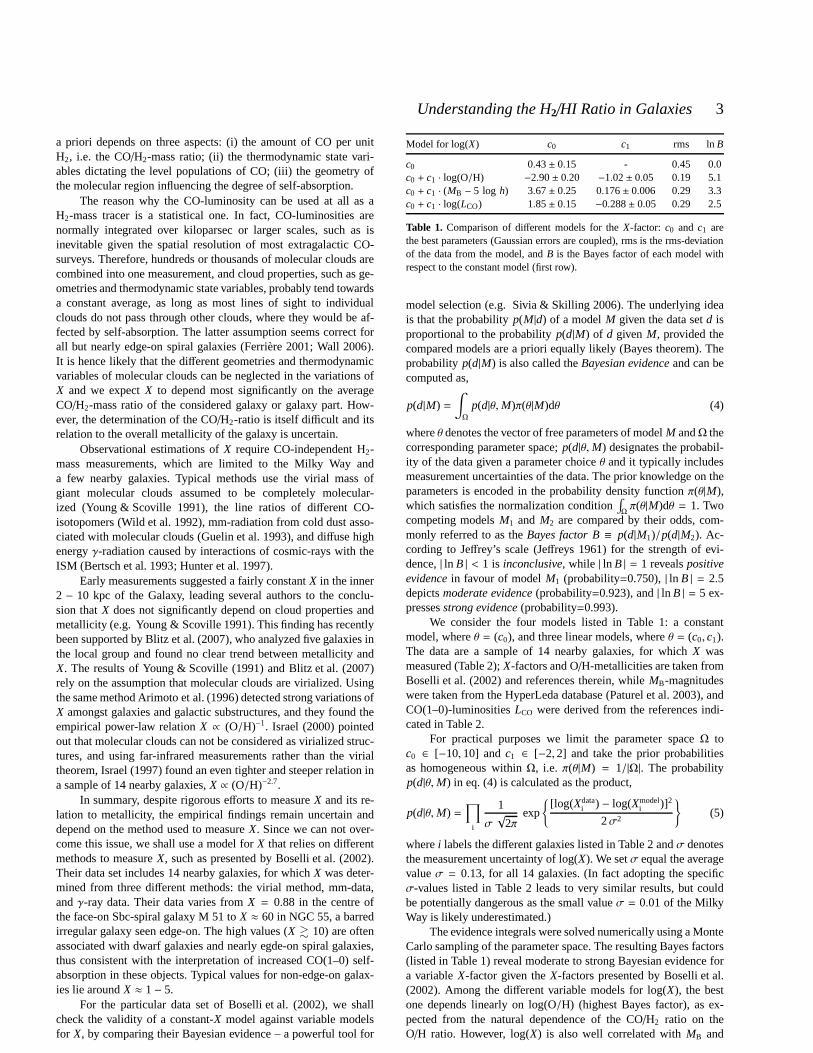
Model for log(X) c0 c1 rms lnB

c0 0.43± 0.15 - 0.45 0.0c0 + c1 · log(O/H) −2.90± 0.20 −1.02± 0.05 0.19 5.1c0 + c1 · (MB − 5 log h) 3.67± 0.25 0.176± 0.006 0.29 3.3c0 + c1 · log(LCO) 1.85± 0.15 −0.288± 0.05 0.29 2.5

Table 1. Comparison of different models for theX-factor: c0 and c1 arethe best parameters (Gaussian errors are coupled), rms is the rms-deviationof the data from the model, andB is the Bayes factor of each model withrespect to the constant model (first row).

model selection (e.g. Sivia & Skilling 2006). The underlying ideais that the probabilityp(M|d) of a modelM given the data setd isproportional to the probabilityp(d|M) of d given M, provided thecompared models are a priori equally likely (Bayes theorem). Theprobability p(d|M) is also called theBayesian evidence and can becomputed as,

p(d|M) =∫

Ω

p(d|θ,M)π(θ|M)dθ (4)

whereθ denotes the vector of free parameters of modelM andΩ thecorresponding parameter space;p(d|θ,M) designates the probabil-ity of the data given a parameter choiceθ and it typically includesmeasurement uncertainties of the data. The prior knowledgeon theparameters is encoded in the probability density functionπ(θ|M),which satisfies the normalization condition

∫

Ωπ(θ|M)dθ = 1. Two

competing modelsM1 and M2 are compared by their odds, com-monly referred to as theBayes factor B ≡ p(d|M1)/p(d|M2). Ac-cording to Jeffrey’s scale (Jeffreys 1961) for the strength of evi-dence,| ln B | < 1 is inconclusive, while | ln B | = 1 revealspositiveevidence in favour of modelM1 (probability=0.750),| ln B | = 2.5depictsmoderate evidence (probability=0.923), and| ln B | = 5 ex-pressesstrong evidence (probability=0.993).

We consider the four models listed in Table 1: a constantmodel, whereθ = (c0), and three linear models, whereθ = (c0, c1).The data are a sample of 14 nearby galaxies, for whichX wasmeasured (Table 2);X-factors and O/H-metallicities are taken fromBoselli et al. (2002) and references therein, whileMB-magnitudeswere taken from the HyperLeda database (Paturel et al. 2003), andCO(1–0)-luminositiesLCO were derived from the references indi-cated in Table 2.

For practical purposes we limit the parameter spaceΩ toc0 ∈ [−10, 10] andc1 ∈ [−2,2] and take the prior probabilitiesas homogeneous withinΩ, i.e. π(θ|M) = 1/|Ω|. The probabilityp(d|θ,M) in eq. (4) is calculated as the product,

p(d|θ,M) =∏

i

1

σ√

2πexp

[log(Xdatai ) − log(Xmodel

i )]2

2σ2

(5)

wherei labels the different galaxies listed in Table 2 andσ denotesthe measurement uncertainty of log(X). We setσ equal the averagevalueσ = 0.13, for all 14 galaxies. (In fact adopting the specificσ-values listed in Table 2 leads to very similar results, but couldbe potentially dangerous as the small valueσ = 0.01 of the MilkyWay is likely underestimated.)

The evidence integrals were solved numerically using a MonteCarlo sampling of the parameter space. The resulting Bayes factors(listed in Table 1) reveal moderate to strong Bayesian evidence fora variableX-factor given theX-factors presented by Boselli et al.(2002). Among the different variable models for log(X), the bestone depends linearly on log(O/H) (highest Bayes factor), as ex-pected from the natural dependence of the CO/H2 ratio on theO/H ratio. However, log(X) is also well correlated withMB and

c© 2008 RAS, MNRAS000, 1–20

4 D. Obreschkow and S. Rawlings

Object log(O/H) (a) M (b)B log(LCO) log(X) (a)

−5 log h

SMC -3.96 -16.82 -2.04(c) 1.00NGC1569 -3.81 -15.94 -1.60(d) 1.18M31 -2.99 -20.23 -1.40(e) 0.38± 0.21IC10 -3.69 -15.13 -1.09(f) 0.82± 0.12LMC -3.63 -17.63 -0.68(g) 0.90M81 -3 -19.90 -0.07(h) -0.15M33 -3.22 -18.61 0.20(i) 0.70± 0.11M82 -3 -17.30 0.67(d) 0.00NGC4565 - -21.74 1.12(h) 0.00NGC6946 -2.94 -20.12 1.24(h) 0.26NGC891 - -19.43 1.48(h) 0.18M51 -2.77 -19.74 1.80(h) -0.22Milky Way -3.1 -19.63 - 0.19± 0.01NGC6822 -3.84 -16.07 - 0.82± 0.20

Table 2. Observational data used for the derivation of a variableX-factor (Section 2.2).LCO is given in units of Jy km s−1 (h−1 Mpc)2.(a) O/H-metallicities andX-factors from Boselli et al. (2002), (b) ab-solute, extinction-corrected B-Magnitudes from the HyperLeda database(Paturel et al. 2003), (c) Rubio et al. (1991), (d) Young et al. (1989), (e)Heyer et al. (2000), (f) Leroy et al. (2006), (g) Fukui et al. (1999), (h) Sage(1993), (i) Heyer et al. (2004).

log(LCO), and hereafter we will use those relations because of thewidespread availability ofMB andLCO data. In fact, aX-factor de-pending onLCO simply translates to a non-linear conversion of CO-luminosities into H2-masses. If the two linear regressions betweenlog(X) andMB and between log(X) and log(LCO) were determinedindependently, they would imply a third linear relation betweenMB

and log(LCO). The later can, however, be determined more accu-rately from larger galaxy samples. The sample presented in Section4.1 (245 galaxies) yields

log(LCO) ≈ −4.5− 0.52 (MB − 5 log h), (6)

whereLCO is taken in units of Jy km s−1 (h−1 Mpc)2. To get the bestresult, we imposed this relation, while simultaneously minimizingthe square deviations of the two regressions between log(X) andrespectivelyMB and log(LCO). In such a way we find

log(X) = 1.97− 0.308 log(LCO) ± σX , (7)

log(X) = 3.36+ 0.160 (MB − 5 log h) ± σX . (8)

These two relations are shown in Fig. 2 (red solid lines). Forcom-parison the independent regressions, obtained without imposing therelation given in eq. (6), are plotted as dashed lines. Theserelationscorrespond to the parametersc0 andc1 given in Table 1. Other re-gressions found by Arimoto et al. (1996) and Boselli et al. (2002)are also displayed. Their approaches are similar, but Arimoto et al.(1996) used less galaxies (8 instead of 14). The 14 data points inFig. 2 are scattered around the relations of eqs. (7) and (8) with thesame rms-deviation of 0.29 in log(X). Combined with the averagemeasurement uncertainty ofσ = 0.13, this gives an estimated truephysical scatter in log(X) of σX = (0.292 − 0.132)1/2 = 0.26.

The variable models ofX given in eqs. (7) and (8) will be ap-plied in Sections 3 and 4. In order to account for the uncertainties ofX highlighted in the beginning of this section, we shall also presentthe results for a constantX-factor with random scatter in Section 3.

-21 -19 -17 -15

N1569

M31

M81

M33

M51

N891

-1

0

1

2

3 4 5

N6946

LMCIC10SMC

N4565

M82 N4565

M31

M81M51

MWN891

M33

LMC

M82

SMC

IC10

N6822

N1569

log(

)X

log( Mpc ])L hCO-1 -2 2/ [Jy km s M hB - 5 log

2

N6946

Figure 2. Points represent observedX-factors as a function of CO(1–0)-power LCO and absolute blue magnitudeMB for 14 local galaxies. Redsolid lines represent linear regressions respecting the mutual relation be-tween LCO and MB given in eq. (6); dashed lines represent indepen-dent linear regressions; the dotted line represents the linear fit found byArimoto et al. (1996); and the dash-dotted line represents the linear fit foundby Boselli et al. (2002).

3 DERIVING THE H 2-MF FROM THE CO-LF

Using the variable model for theX-factor of eq. (7), we shall nowrecover the local H2-mass function (H2-MF) from the CO-LF pre-sented by Keres et al. (2003). The latter is based on a far infrared-selected subsample of 200 galaxies from the FCRAO ExtragalacticCO-Survey (Young et al. 1995), which successfully reproduced the60µm-LF, thus limiting the errors caused by the incompletenessofthe sample. Keres et al. (2003) themselves derived a H2-MF usinga constant modelX = 3, which probably leads to an overestimationof the H2-abundance, especially in the high mass end, where theX-factors tend to be lower according to the data shown in Section2.2.

We applied eq. (7) with scatterσX = 0.26 to the individualdata points of the CO-LF given by Keres et al. (2003). The result-ing H2-MF – hereafter thereference H2-MF – is shown in Fig. 3together with theoriginal H2-MF derived by Keres et al. (2003)using the constant factorX = 3 without scatter. To both functionswe fitted a Schechter function (Schechter 1976) of the form

φH2 = ln(10) · φ∗ ·(

MH2

M∗

)α+1

exp

[

−(

MH2

M∗

)]

(9)

by minimising the weighted square deviations of all but the highestH2-mass bin. Keres et al. (2003) argue that this bin may containaCO-luminous subpopulation of starburst galaxies, similarly to thesituation in the far infrared continuum (Yun et al. 2001). Inany casethe last bin only marginally contributes to the universal H2-density.The Schechter function parameters are given in Table 3, as well asthe reducedχ2 of the fits, total H2-densitiesρH2 andΩH2 ≡ ρH2/ρcrit,and the average molecular ratioηuniverse≡ ΩH2/ΩHI. BothρH2 andΩH2 were evaluated from the fitted Schechter function rather thanthe binned data, andΩHI = (2.6 ± 0.3) h−110−4 was adopted fromthe HIPASS analysis by Zwaan et al. (2005).

Our new reference H2-MF is compressed in the mass-axiscompared to the original one, and our estimate ofρH2 (Table 3) is 33per cent smaller. The global H2/HI-mass ratio drops to 0.26± 0.11,implying a total cold gas density ofΩgas = (4.4 ± 0.8) · 10−4 h−1.The composition of cold gas becomes: 59± 6 per cent HI, 15± 6

c© 2008 RAS, MNRAS000, 1–20

Understanding the H2/HI Ratio in Galaxies 5

-6

-5

-4

-3

-2

-1

6.5 7.0 7.5 8.0 8.5 9.0 9.5 10.0 10.5

log( ])MH2/ [h-2 M

log

(M

pc

])H

2/ [

-3h

3ff

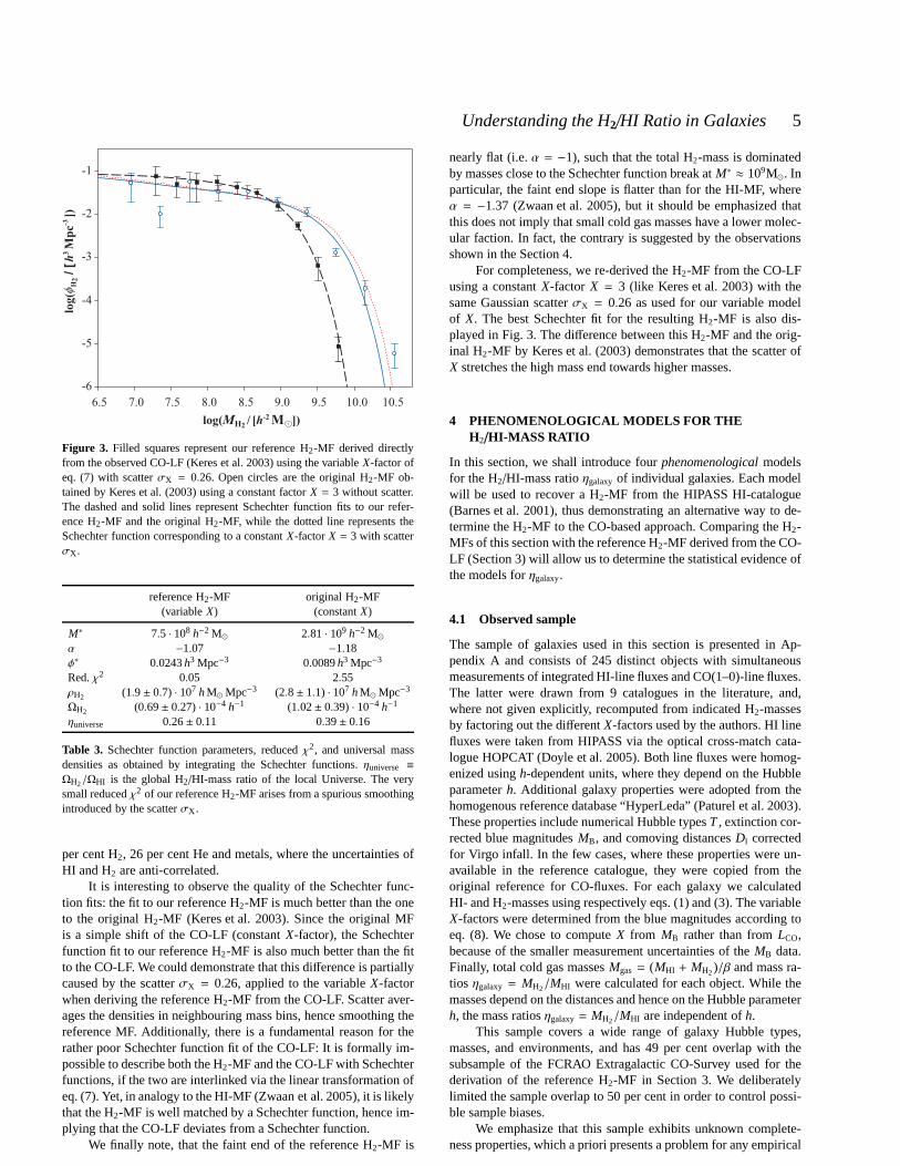
Figure 3. Filled squares represent our reference H2-MF derived directlyfrom the observed CO-LF (Keres et al. 2003) using the variable X-factor ofeq. (7) with scatterσX = 0.26. Open circles are the original H2-MF ob-tained by Keres et al. (2003) using a constant factorX = 3 without scatter.The dashed and solid lines represent Schechter function fitsto our refer-ence H2-MF and the original H2-MF, while the dotted line represents theSchechter function corresponding to a constantX-factorX = 3 with scatterσX .

reference H2-MF original H2-MF(variableX) (constantX)

M∗ 7.5 · 108 h−2 M⊙ 2.81 · 109 h−2 M⊙α −1.07 −1.18φ∗ 0.0243h3 Mpc−3 0.0089h3 Mpc−3

Red.χ2 0.05 2.55ρH2 (1.9± 0.7) · 107 h M⊙Mpc−3 (2.8± 1.1) · 107 h M⊙Mpc−3

ΩH2 (0.69± 0.27) · 10−4 h−1 (1.02± 0.39) · 10−4 h−1

ηuniverse 0.26± 0.11 0.39± 0.16

Table 3. Schechter function parameters, reducedχ2, and universal massdensities as obtained by integrating the Schechter functions. ηuniverse ≡ΩH2/ΩHI is the global H2/HI-mass ratio of the local Universe. The verysmall reducedχ2 of our reference H2-MF arises from a spurious smoothingintroduced by the scatterσX .

per cent H2, 26 per cent He and metals, where the uncertainties ofHI and H2 are anti-correlated.

It is interesting to observe the quality of the Schechter func-tion fits: the fit to our reference H2-MF is much better than the oneto the original H2-MF (Keres et al. 2003). Since the original MFis a simple shift of the CO-LF (constantX-factor), the Schechterfunction fit to our reference H2-MF is also much better than the fitto the CO-LF. We could demonstrate that this difference is partiallycaused by the scatterσX = 0.26, applied to the variableX-factorwhen deriving the reference H2-MF from the CO-LF. Scatter aver-ages the densities in neighbouring mass bins, hence smoothing thereference MF. Additionally, there is a fundamental reason for therather poor Schechter function fit of the CO-LF: It is formally im-possible to describe both the H2-MF and the CO-LF with Schechterfunctions, if the two are interlinked via the linear transformation ofeq. (7). Yet, in analogy to the HI-MF (Zwaan et al. 2005), it islikelythat the H2-MF is well matched by a Schechter function, hence im-plying that the CO-LF deviates from a Schechter function.

We finally note, that the faint end of the reference H2-MF is

nearly flat (i.e.α = −1), such that the total H2-mass is dominatedby masses close to the Schechter function break atM∗ ≈ 109M⊙. Inparticular, the faint end slope is flatter than for the HI-MF,whereα = −1.37 (Zwaan et al. 2005), but it should be emphasized thatthis does not imply that small cold gas masses have a lower molec-ular faction. In fact, the contrary is suggested by the observationsshown in the Section 4.

For completeness, we re-derived the H2-MF from the CO-LFusing a constantX-factor X = 3 (like Keres et al. 2003) with thesame Gaussian scatterσX = 0.26 as used for our variable modelof X. The best Schechter fit for the resulting H2-MF is also dis-played in Fig. 3. The difference between this H2-MF and the orig-inal H2-MF by Keres et al. (2003) demonstrates that the scatter ofX stretches the high mass end towards higher masses.

4 PHENOMENOLOGICAL MODELS FOR THEH2/HI-MASS RATIO

In this section, we shall introduce fourphenomenological modelsfor the H2/HI-mass ratioηgalaxy of individual galaxies. Each modelwill be used to recover a H2-MF from the HIPASS HI-catalogue(Barnes et al. 2001), thus demonstrating an alternative wayto de-termine the H2-MF to the CO-based approach. Comparing the H2-MFs of this section with the reference H2-MF derived from the CO-LF (Section 3) will allow us to determine the statistical evidence ofthe models forηgalaxy.

4.1 Observed sample

The sample of galaxies used in this section is presented in Ap-pendix A and consists of 245 distinct objects with simultaneousmeasurements of integrated HI-line fluxes and CO(1–0)-linefluxes.The latter were drawn from 9 catalogues in the literature, and,where not given explicitly, recomputed from indicated H2-massesby factoring out the differentX-factors used by the authors. HI linefluxes were taken from HIPASS via the optical cross-match cata-logue HOPCAT (Doyle et al. 2005). Both line fluxes were homog-enized usingh-dependent units, where they depend on the Hubbleparameterh. Additional galaxy properties were adopted from thehomogenous reference database “HyperLeda” (Paturel et al.2003).These properties include numerical Hubble typesT , extinction cor-rected blue magnitudesMB, and comoving distancesDl correctedfor Virgo infall. In the few cases, where these properties were un-available in the reference catalogue, they were copied fromtheoriginal reference for CO-fluxes. For each galaxy we calculatedHI- and H2-masses using respectively eqs. (1) and (3). The variableX-factors were determined from the blue magnitudes according toeq. (8). We chose to computeX from MB rather than fromLCO,because of the smaller measurement uncertainties of theMB data.Finally, total cold gas massesMgas = (MHI + MH2)/β and mass ra-tios ηgalaxy = MH2/MHI were calculated for each object. While themasses depend on the distances and hence on the Hubble parameterh, the mass ratiosηgalaxy= MH2/MHI are independent ofh.

This sample covers a wide range of galaxy Hubble types,masses, and environments, and has 49 per cent overlap with thesubsample of the FCRAO Extragalactic CO-Survey used for thederivation of the reference H2-MF in Section 3. We deliberatelylimited the sample overlap to 50 per cent in order to control possi-ble sample biases.

We emphasize that this sample exhibits unknown complete-ness properties, which a priori presents a problem for any empirical

c© 2008 RAS, MNRAS000, 1–20

6 D. Obreschkow and S. Rawlings

-2

-1

0

1

-5 0 5 10Morph. Type T

-1.3

log

(gala

xy

H2

HI

M)

=lo

g(

/)

Mh

E E/S0 S0 S0/a Sa Sab Sb Sbc Sc Scd Sd Sm Irr

h

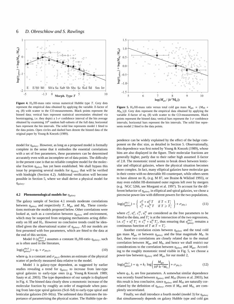
Figure 4. H2/HI-mass ratio versus numerical Hubble typeT . Grey dotsrepresent the empirical data obtained by applying the variable X-factor ofeq. (8) with scatter to the CO-measurements. Black points represent thebinned data; vertical bars represent statistical uncertainties obtained viabootstrapping, i.e. they depict a 1-σ confidence interval of the bin averageobtained by examining 104 random half-subsets of the full data; horizontalbars represent the bin intervals. The solid line representsmodel 1 fitted tothe data points. Open circles and dashed bars denote the binned data of theoriginal paper by Young & Knezek (1989).

model forηgalaxy. However, as long as a proposed model is formallycomplete in the sense that it embodies the essential correlationswith a set of free parameters, these parameters can be determinedaccurately even with an incomplete set of data points. The difficultyin the present case is that no reliable complete model for themolec-ular fractionηgalaxy has yet been established. We shall bypass thisissue by proposing several models forηgalaxy that will be verifiedwith hindsight (Section 4.2). Additional verification willbecomepossible in Section 5, where we shall derive a physical modelforηgalaxy.

4.2 Phenomenological models forηgalaxy

The galaxy sample of Section 4.1 reveals moderate correlationsbetweenηgalaxy and respectivelyT , Mgas and MB. These correla-tions motivate the models proposed below. Other correlations werelooked at, such as a correlation betweenηgalaxy and environment,which may be suspected from stripping mechanisms acting differ-ently on HI and H2. However no conclusive trends could be iden-tified given the observational scatter ofηgalaxy. All our models arefirst presented with free parameters, which are fitted to the data atthe end of this section.

Model 0 (ηobs,0galaxy) assumes a constant H2/HI-ratio ηgalaxy, such

as is often used in the literature,

log(ηobs,0galaxy) = q0 + σphy,0, (10)

whereq0 is a constant andσphy,0 denotes an estimate of the physicalscatter of perfectly measured data relative to the model.

Model 1 is galaxy-type dependent, as suggested by earlierstudies revealing a trend forηgalaxy to increase from late-typespiral galaxies to early-type ones (e.g. Young & Knezek 1989;Sauty et al. 2003). The type dependence of our sample is displayedin Fig. 4. The binned data clearly show a monotonic increase of themolecular fraction by roughly an order of magnitude when pass-ing from late-type spiral galaxies (Scd–Sd) to early-type spiral andlenticular galaxies (S0–S0/a). The unbinned data illustrates the im-portance of parametrising the physical scatter. The Hubbletype de-

-1.5

-1.0

-0.5

0.0

0.5

1.0

1.5

5 6 7 8 9 10

log( / [ ])Mgas h-2M

log

(g

ala

xy

H2

HI

M)

=lo

g(

/)

Mhh

Figure 5. H2/HI-mass ratio versus total cold gas massMgas ≡ (MHI +

MH2)/β. Grey dots represent the empirical data obtained by applying thevariable X-factor of eq. (8) with scatter to the CO-measurements. Blackpoints represent the binned data; vertical bars represent the 1-σ confidenceintervals; horizontal bars represent the bin intervals. The solid line repre-sents model 2 fitted to the data points.

pendence can be widely explained by the effect of the bulge com-ponent on the disc size, as detailed in Section 5. Observationally,this dependence was first noted by Young & Knezek (1989), whosebins are also displayed in the figure. Their molecular fractions aregenerally higher, partly due to their rather high assumedX-factorof 2.8. The monotonic trend seems to break down between lentic-ular and elliptical galaxies, where the physical situationbecomesmore complex. In fact, many elliptical galaxies have molecular gasin their centre with no detectable HI-counterpart, while others seemto have almost no H2 (e.g. M 87, see Braine & Wiklind 1993), ormay even exhibit HI-dominated outer regions left over by mergers(e.g. NGC 5266, see Morganti et al. 1997). To account for the dif-ferent behavior ofηgalaxy in elliptical and spiral galaxies, we chose apiecewise power-law with different powers for the two populations,

log(ηobs,1galaxy) =

cel1 + uel

1 T if T < T ∗1csp

1 + usp1 T if T > T ∗1

+ σphy,1 (11)

wherecel1 , uel

1 , csp1 , usp

1 are considered as the free parameters to befitted to the data, andT ∗1 is at the intersection of the two regressions,i.e. cel

1 + uel1 T ∗1 ≡ csp

1 + usp1 T ∗1, thus ensuring thatηobs,1

galaxy remains acontinuous function ofT at T = T ∗1.

Another correlation exists betweenηgalaxy and the total coldgas massMgas or betweenηgalaxy and the blue magnitudeMB. Infact, these two correlations are closely related due to the mutualcorrelation betweenMgas and MB, and hence we shall restrict ourconsiderations to the correlation betweenηgalaxy andMgas. Accord-ing to the roughly monotonic trend visible in Fig. 5, we choose apower-law betweenηgalaxy andMgas for our model 2,

log(ηobs,2galaxy) = q2 + k2 log

(

Mgas

109 h−2M⊙

)

+ σphy,2, (12)

whereq2, k2 are free parameters. A somewhat similar dependencewas recently found betweenηgalaxy andMHI (Keres et al. 2003), butthis result is less conclusive, sinceηgalaxy andMHI are naturally cor-related by the definition ofηgalaxy, even if MHI and MH2 are com-pletely uncorrelated.

Finally, we shall introduce a fourth model (model 3) forηgalaxy

that simultaneously depends on galaxy Hubble type and cold gas

c© 2008 RAS, MNRAS000, 1–20

Understanding the H2/HI Ratio in Galaxies 7

Model log(ηobs,igalaxy) i = 0 i = 1 i = 2 i = 3

qi −0.58+0.16−0.23 - −0.51+0.03

−0.04 -

celi - +0.18+0.40

−0.22 - −0.01+0.25−0.16

ueli - +0.12+0.14

−0.05 - +0.13+0.07−0.04

cspi - −0.14+0.10

−0.07 - −0.02+0.10−0.09

uspi - −0.12+0.01

−0.02 - −0.13+0.02−0.02

ki - - −0.24+0.05−0.05 −0.18+0.06

−0.07

T ∗i - −1.3+1.2−0.5 - −0.1+1.2

−0.6

σdata,i 0.71 0.66 0.67 0.62σphy,i 0.39 0.27 0.30 0.15

Table 4. The upper panel lists the most likely parameters and 1-σ confi-dence intervals of the four modelsηobs,i

galaxy (i = 0, ...,3). The bottom panelshows the rms-deviationsσdata,i of the data from the model predictions andthe estimated physical scatterσphy,i for each modeli.

mass,

log(ηobs,3galaxy) =

cel3 +uel

3 T (if T < T∗3)csp

3 +usp3 T (if T > T∗3)

(13)

+k3 log

(

Mgas

109 h−2M⊙

)

+ σphy,3 ,

wherecel3 , uel

3 , csp3 , usp

3 , k3 are free parameters andT ∗3 is defined ascel

3 + uel3 T ∗3 ≡ csp

3 + usp3 T ∗3, thus makingηobs,3

galaxy a continuous functionof T at T = T ∗3. Comparing this model with models 1 and 2, willalso allow us to study a possible degeneracy between model 1 andmodel 2 caused by a dependence between cold gas mass and galaxyHubble type.

The free parameters of the above models were determined byminimizing the rms-deviation between the model predictions andthe 245 observed values of log(ηgalaxy) (Appendix A). Optimizationin log-space is the most sensible choice sinceηgalaxy is subject toGaussian scatter in log-space as will be shown in the Section4.3.The most probable values of all parameters are shown in Table4together with the corresponding 1-σ confidence intervals. The lat-ter were obtained using a bootstrapping method that uses 104 ran-dom half-sized subsamples of the full data set and determines themodel-parameters for every one of them. The resulting distributionof values for each free parameter was approximated by a Gaussiandistribution and its standard deviationσ was divided by

√2 in or-

der to find the 1-σ confidence intervals for the full data set. Notethat in some cases the parameter uncertainties are coupled,i.e. achange in one parameter can be accommodated by changing theothers, such that the model remains nearly identical. For models 1and 2, the best fits are displayed in Figs. 4 and 5 as solid lines.

Table 4 also shows different scatters that will be explained inSection 4.3.

4.3 Scatter and uncertainty

The empirical values ofηgalaxy scatter around the model predictionsaccording to the distributions shown in Fig. 6 (dashed lines). Theclose similarity of these distributions to Gaussians in log-space(solid lines) allows us to consider the rms-deviations of the dataσdata as the standard deviations of a Gaussians. This exhibits theadvantage thatσdata can be decomposed in model-independent ob-servational scatterσobs and model-dependent physical scatterσphy

via the square-sum relationσ2data,i = σ

2obs+ σ

2phy,i , i = 0, ...,3.

The major contribution toσdata,i comes from observational

0

0.2

0.4

0.6

-2.0 -1.0 0.0 1.0 2.0

Norm

ali

zed

fre

qu

ency

Deviation from model = log( galaxy ga`laxy) – log( )h h

Model 0

Model 2

Model 1

Model 3

h hobs,i

Figure 6. Distributions of the deviations between the observed values oflog(ηgalaxy) and the model-values log(ηobs,i

galaxy) (i = 1, ...,3). Data points anddashed lines represent the actual distribution of the data;solid lines repre-sent Gaussian distributions with equal standard deviations.

scatter, as suggested by the close similarity of the different valuesof σdata,i . Indeed, the observational scatter inferred from theηgalaxy

values of the 22 repeated sources in our data isσobs ≈ 0.6. Thisscatter is a combination of CO-flux measurement uncertainties, un-certain CO/H2-conversions and HI-flux uncertainties (in decreas-ing significance). Sinceσobs is only marginally smaller thanσdata,i

for all models, the estimation of the physical scattersσphy,i (givenin Table 4) is uncertain. Nevertheless, we shall include these bestguesses of the physical scatter, when constructing the H2-MFs inSection 4.4.

4.4 Recovering the H2-MF and model evidence

Given a model forηgalaxy, H2-masses of arbitrary HI-galaxies can beestimated. We shall apply this technique to the 4315 sourcesin theHIPASS catalogue using our four models ofηobs,i

galaxy, i = 0, ...,3. Foreach model, the resulting H2-catalogue with 4315 objects will beconverted into a H2-MF, which can be compared to our referenceH2-MF derived directly from the CO-LF (Section 3).

For the modelsηobs,1galaxy(T ) andηobs,3

galaxy(Mgas, T ) Hubble typesTwere drawn from the HyperLeda database for each galaxy in theHIPASS catalogue by means of the galaxy identifiers given in theoptical cross-match catalogue HOPCAT (Doyle et al. 2005). H2-masses were then computed viaMH2 = η

obs,igalaxy MHI, i = 0, ...,3.

This equation is implicit in case of the mass-dependent modelsηobs,2

galaxy(Mgas) and ηobs,3galaxy(Mgas,T ), where Mgas = (MHI + MH2)/β.

All four models were applied with scatter, randomly drawn froma Gaussian distribution with the model-specific scatterσphy,i, listedin Table 4.

In order to reconstruct a H2-MF for each model, we employedthe 1/Vmax method (Schmidt 1968), whereVmax was calculatedfrom the analytic completeness function for HIPASS that dependson the HI peak flux densityS p, the integrated HI line fluxS int, andthe flux limit of the survey (Zwaan et al. 2004). After ensuring thatwe can accurately reproduce the HI-MF derived by Zwaan et al.(2005), we evaluated the four H2-MFs (one for each modelηobs,i

galaxy)displayed in Fig. 7 (dots). The uncertainties of log(φH2) vary aroundσ = 0.03− 0.1. Each function was fitted by a Schechter functionby minimizing the weighted rms-deviation (coloured solid lines).

The comparison of these four H2-MFs with the reference H2-

c© 2008 RAS, MNRAS000, 1–20

8 D. Obreschkow and S. Rawlings

log( )MH2/[ ]h

-2 M

7.0 7.5 8.0 8.5 9.0 9.5 10.0 10.5

Model 0

Model 1

Model 2

Model 3

-7

-6

-5

-4

-3

-2

-1

0

log(

H2/ [h

3M

pc

])-3

ff

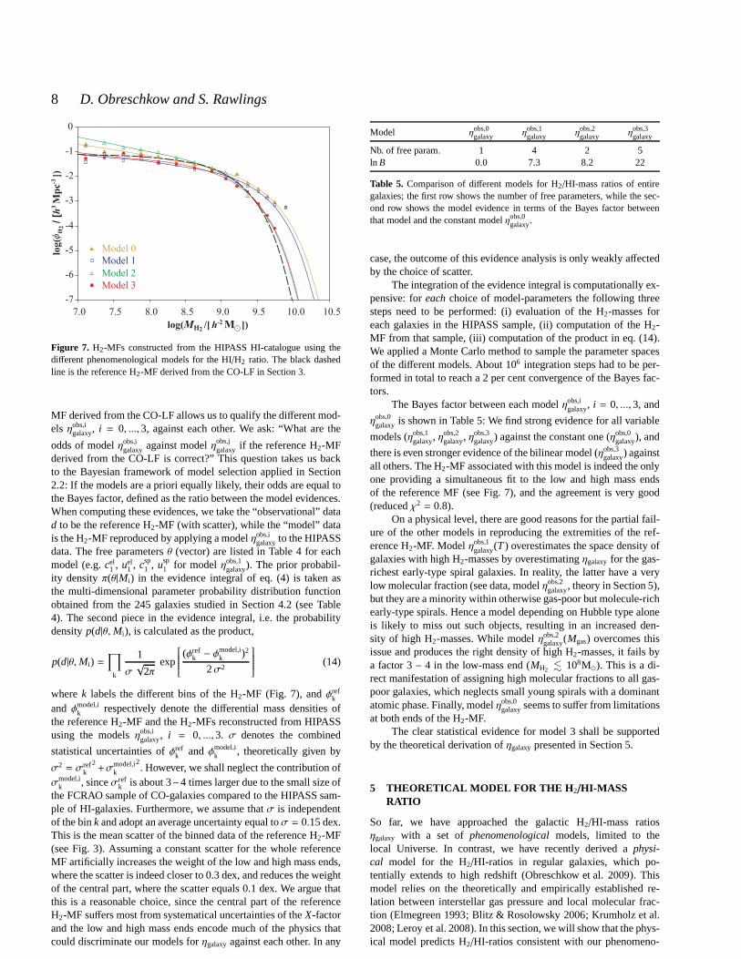
Figure 7. H2-MFs constructed from the HIPASS HI-catalogue using thedifferent phenomenological models for the HI/H2 ratio. The black dashedline is the reference H2-MF derived from the CO-LF in Section 3.

MF derived from the CO-LF allows us to qualify the different mod-els ηobs,i

galaxy, i = 0, ...,3, against each other. We ask: “What are the

odds of modelηobs,igalaxy against modelηobs,j

galaxy if the reference H2-MFderived from the CO-LF is correct?” This question takes us backto the Bayesian framework of model selection applied in Section2.2: If the models are a priori equally likely, their odds areequal tothe Bayes factor, defined as the ratio between the model evidences.When computing these evidences, we take the “observational” datad to be the reference H2-MF (with scatter), while the “model” datais the H2-MF reproduced by applying a modelηobs,i

galaxy to the HIPASSdata. The free parametersθ (vector) are listed in Table 4 for eachmodel (e.g.cel

1 , uel1 , csp

1 , usp1 for modelηobs,1

galaxy). The prior probabil-ity densityπ(θ|Mi) in the evidence integral of eq. (4) is taken asthe multi-dimensional parameter probability distribution functionobtained from the 245 galaxies studied in Section 4.2 (see Table4). The second piece in the evidence integral, i.e. the probabilitydensityp(d|θ,Mi), is calculated as the product,

p(d|θ,Mi) =∏

k

1

σ√

2πexp

(φrefk − φ

model,ik )2

2σ2

(14)

wherek labels the different bins of the H2-MF (Fig. 7), andφrefk

and φmodel,ik respectively denote the differential mass densities of

the reference H2-MF and the H2-MFs reconstructed from HIPASSusing the modelsηobs,i

galaxy, i = 0, ...,3. σ denotes the combined

statistical uncertainties ofφrefk andφmodel,i

k , theoretically given by

σ2 = σrefk

2+σmodel,i

k

2. However, we shall neglect the contribution of

σmodel,ik , sinceσref

k is about 3−4 times larger due to the small size ofthe FCRAO sample of CO-galaxies compared to the HIPASS sam-ple of HI-galaxies. Furthermore, we assume thatσ is independentof the bink and adopt an average uncertainty equal toσ = 0.15 dex.This is the mean scatter of the binned data of the reference H2-MF(see Fig. 3). Assuming a constant scatter for the whole referenceMF artificially increases the weight of the low and high mass ends,where the scatter is indeed closer to 0.3 dex, and reduces theweightof the central part, where the scatter equals 0.1 dex. We argue thatthis is a reasonable choice, since the central part of the referenceH2-MF suffers most from systematical uncertainties of theX-factorand the low and high mass ends encode much of the physics thatcould discriminate our models forηgalaxy against each other. In any

Model ηobs,0galaxy η

obs,1galaxy η

obs,2galaxy η

obs,3galaxy

Nb. of free param. 1 4 2 5ln B 0.0 7.3 8.2 22

Table 5. Comparison of different models for H2/HI-mass ratios of entiregalaxies; the first row shows the number of free parameters, while the sec-ond row shows the model evidence in terms of the Bayes factor betweenthat model and the constant modelηobs,0

galaxy.

case, the outcome of this evidence analysis is only weakly affectedby the choice of scatter.

The integration of the evidence integral is computationally ex-pensive: foreach choice of model-parameters the following threesteps need to be performed: (i) evaluation of the H2-masses foreach galaxies in the HIPASS sample, (ii) computation of the H2-MF from that sample, (iii) computation of the product in eq. (14).We applied a Monte Carlo method to sample the parameter spacesof the different models. About 106 integration steps had to be per-formed in total to reach a 2 per cent convergence of the Bayes fac-tors.

The Bayes factor between each modelηobs,igalaxy, i = 0, ...,3, and

ηobs,0galaxy is shown in Table 5: We find strong evidence for all variable

models (ηobs,1galaxy, η

obs,2galaxy, η

obs,3galaxy) against the constant one (ηobs,0

galaxy), and

there is even stronger evidence of the bilinear model (ηobs,3galaxy) against

all others. The H2-MF associated with this model is indeed the onlyone providing a simultaneous fit to the low and high mass endsof the reference MF (see Fig. 7), and the agreement is very good(reducedχ2 = 0.8).

On a physical level, there are good reasons for the partial fail-ure of the other models in reproducing the extremities of theref-erence H2-MF. Modelηobs,1

galaxy(T ) overestimates the space density ofgalaxies with high H2-masses by overestimatingηgalaxy for the gas-richest early-type spiral galaxies. In reality, the latterhave a verylow molecular fraction (see data, modelηobs,2

galaxy, theory in Section 5),but they are a minority within otherwise gas-poor but molecule-richearly-type spirals. Hence a model depending on Hubble type aloneis likely to miss out such objects, resulting in an increasedden-sity of high H2-masses. While modelηobs,2

galaxy(Mgas) overcomes thisissue and produces the right density of high H2-masses, it fails bya factor 3− 4 in the low-mass end (MH2 . 108M⊙). This is a di-rect manifestation of assigning high molecular fractions to all gas-poor galaxies, which neglects small young spirals with a dominantatomic phase. Finally, modelηobs,0

galaxyseems to suffer from limitationsat both ends of the H2-MF.

The clear statistical evidence for model 3 shall be supportedby the theoretical derivation ofηgalaxy presented in Section 5.

5 THEORETICAL MODEL FOR THE H 2/HI-MASSRATIO

So far, we have approached the galactic H2/HI-mass ratiosηgalaxy with a set of phenomenological models, limited to thelocal Universe. In contrast, we have recently derived aphysi-cal model for the H2/HI-ratios in regular galaxies, which po-tentially extends to high redshift (Obreschkow et al. 2009). Thismodel relies on the theoretically and empirically established re-lation between interstellar gas pressure and local molecular frac-tion (Elmegreen 1993; Blitz & Rosolowsky 2006; Krumholz et al.2008; Leroy et al. 2008). In this section, we will show that the phys-ical model predicts H2/HI-ratios consistent with our phenomeno-

c© 2008 RAS, MNRAS000, 1–20

Understanding the H2/HI Ratio in Galaxies 9

logical model 3 given in eq. (13). Hence the physical (or “theo-retical”) model provides a reliable explanation for the global phe-nomenology of the H2/HI-ratio in galaxies.

5.1 Background: theη–pressure relation

Understanding the observed continuous variation ofη within indi-vidual galaxies (e.g. Leroy et al. 2008) requires some explanation,since, fundamentally, there is no mixed thermodynamic equilib-rium of HI and H2. To first order, the ISM outside molecular cloudsis atomic, while a cloud-region in local thermodynamic equilib-rium (LTE) is either fully atomic or fully molecular, depending onthe local state variables. The apparent continuous variation of η isthe combined result of (i) a non-resolved conglomeration offullyatomic and fully molecular clouds, (ii) clouds with molecular coresand atomic shells in different LTE, and (iii) some cloud regionsoff LTE with actual transient mixtures of HI and H2. However, atime-dependent model for off-equilibrium clouds (Goldsmith et al.2007) revealed that the characteristic time taken between the on-set of cloud compression and full molecularization is of theorderof 107 yrs, much smaller than the typical age of molecular clouds,and hence the fraction of these clouds is small. Therefore, averagedover galactic parts (hundreds or thousands of clouds),η is dictatedby clouds in LTE, entirely defined by a number of state variables.

A theoretical frame exploiting the LTE of molecular cloudswas introduced by Elmegreen (1993), who considered an ideal-ized double population of homogeneous diffuse clouds and isother-mal self-gravitating clouds, both of which can have atomic andmolecular shells. In this model the molecular mass fractionfmol =

dMH2/d(MHI + MH2) of each cloud depends on the density profileand the photodissociative radiation density from starsj, correctedfor self-shielding by the considered cloud, mutual shielding amongdifferent clouds, and dust extinction. Since the shielding fromthisradiation depends on the gas pressure, Elmegreen (1993) finds thatfmol essentially scales with the external pressureP and photodisso-ciative radiation densityj, approximately followingfmol ∝ P2.2 j−1

with an asymptotic flattening towardsfmol = 1 at highP and lowj. This implies approximatelyη ≡ dMH2/dMHI ∝ P2.2 j−1. As-suming thatj is proportional to the surface density of starsΣstars

and that the stellar velocity dispersionσstarsvaries radially asΣ0.5stars,

Wong & Blitz (2002) and Blitz & Rosolowsky (2004, 2006) findroughly j ∝ P and henceη ∝ Pα with α = 1.2. Recently,Krumholz et al. (2008) have presented a more elaborate theory con-cluding thatα ≈ 0.8. However, the exponentα remains uncertain,thus requiring an empirical determination.

Observationally, Blitz & Rosolowsky (2004, 2006) were thefirst ones to reveal a surprisingly tight power-law relationbetweenpressure and molecular fraction based on a sample of 14 nearbygalaxies including dwarf galaxies, HI-rich galaxies, and H2-richgalaxies. Perhaps the richest observational study published so faris the one by Leroy et al. (2008), who analyzed 23 galaxies of TheHI Nearby Galaxy Survey (THINGS, Walter et al. 2008), for whichH2-densities had been derived from CO-data and star formationdensities. This analysis confirmed the power-law relation

η = (P/P∗)α, (15)

whereP is the local, kinematic midplane pressure of the gas, andP∗ andα are free parameters, whose best fit to the data is given byP∗ = 2.35 · 10−13 Pa andα = 0.8.

5.2 Physical model for the H2/HI-ratio in galaxies

We shall now consider the consequence of the model given ineq. (15) for the H2/HI-ratio of entire galaxies. To this end, we adoptthe models and methods presented in Obreschkow et al. (2009), re-stricting this paragraph to an overview.

First, we note that most cold gas of regular galaxies is nor-mally contained in a disc. This even applies to bulge-dominatedearly-type galaxies, such as suggested by recently presented CO-maps of five nearby elliptical galaxies (Young 2002). Hence,theHI- and H2-distributions of all regular galaxies can be well de-scribed by surface density profilesΣHI(r) andΣH2(r). We assumethat the disc is composed of axially symmetric, thin layers of starsand gas, which follow an exponential density profile with a genericscale lengthrdisc, i.e.

Σdiscstars(r) ∼ Σgas(r) ∼ ΣHI(r) + ΣH2(r) ∼ exp(−r/rdisc), (16)

wherer is the galactocentric radius andΣ denotes the mass col-umn densities of the different components. Next, we adopt the phe-nomenological relation of eq. (15), i.e.

ΣHI(r)ΣH2(r)

= [P(r)/P∗]α, (17)

and substitute the kinematic midplane pressureP(r) for (Elmegreen1989)

P(r) =π

2G Σgas(r)

(

Σgas(r) + f Σdiscstars(r)

)

, (18)

whereG is the gravitational constant andf ≡ σgas,z/σstars,z is theratio between the vertical velocity dispersions of gas and stars. Weadopt f = 0.4 according to Elmegreen (1989).

Eqs. (16, 17) can be solved forΣHI (r) and ΣH2(r). InObreschkow et al. (2009), we demonstrate that the resultingsurfaceprofiles are consistent with the empirical data of the two nearby spi-ral galaxies NGC 5055 and NGC 5194 (Leroy et al. 2008). Integrat-ingΣHI(r) andΣH2(r) over the exponential disc gives the gas massesMHI andMH2, hence providing an estimate of their ratioηgalaxy. An-alytically, ηgalaxy is given by an intricate expression, which is verywell approximated (relative error< 0.02 for all galaxies) by thedouble power-law

ηtheorygalaxy=

(

2.14η−0.406c + 6.09η−1.016

c

)−1, (19)

where

ηc =[

11.3 m4 kg−2 r−4discMgas

(

Mgas+ 0.4 Mdiscstars

)]0.8. (20)

ηc is a dimensionless parameter, which can be interpreted as theH2/HI-ratio at the center of a pure disc galaxy. For typical coldgasmasses of average galaxies (Mgas= 108−1010M⊙) and correspond-ing stellar masses and scale radii,ηc calculated from eq. (20) variesroughly between 0.1 and 50. Hence,ηgalaxy given in eq. (19) variesroughly between 0.01 and 1.

In summary, eqs. (19, 20) represent a theoretical model forηgalaxy, which uses three input parameters: the disc stellar massMdisc

stars, the cold gas massMgas, and the exponential scale radiusrdisc

(see Obreschkow et al. 2009 for a detailed discussion).

5.3 Mapping between theoretical and phenomenologicalmodels

We shall now show that our theoretical model for galactic H2/HI-mass ratios given in eqs. (19, 20) closely matches the best phe-nomenological model given in eq. (13). The mapping between the

c© 2008 RAS, MNRAS000, 1–20

10 D. Obreschkow and S. Rawlings

-1 0 1 2log( )

-2

log(

)

-1

0

gal

axy

theo

ry

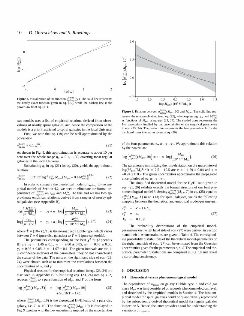
Figure 8. Visualization of the functionηtheorygalaxy(ηc). The solid line represents

the nearly exact function given in eq. (19), while the dashedline is thepower-law fit of eq. (21).

two models uses a list of empirical relations derived from obser-vations of nearby spiral galaxies, and hence the comparisonof themodels is a priori restricted to spiral galaxies in the localUniverse.

First, we note that eq. (19) can be well approximated by thepower-law

ηtheorygalaxy≈ 0.1η0.8

c . (21)

As shown in Fig. 8, this approximation is accurate to about 10percent over the whole rangeηc = 0.1, ...,50, covering most regulargalaxies in the local Universe.

Substitutingηc in eq. (21) for eq. (20), yields the approximaterelation

ηtheorygalaxy=

[

0.31 m4 kg−2 r−4discMgas

(

Mgas+ 0.4 Mdiscstars

)]0.64. (22)

In order to compare the theoretical model ofηgalaxy to the em-pirical models of Section 4.2, we need to eliminate the formal de-pendence ofηtheory

galaxy on rdisc and Mdiscstars. To this end we use two ap-

proximate empirical relations, derived from samples of nearby spi-ral galaxies (see Appendix B),

log

(

Mdiscstars

h−2M⊙

)

= γ1 + α1 log

(

Mgas

2 · 109 h−2 M⊙

)

, (23)

log

(

rdisc

h−1kpc

)

= γ2 + α2 log

(

Mdiscstars

5 · 109 h−2 M⊙

)

+ δ T , (24)

whereT ≡ (10−T )/16 is the normalized Hubble type, which variesbetweenT = 0 (pure disc galaxies) toT = 1 (pure spheroids).

The parameters corresponding to the bestχ2 fit (AppendixB) areα1 = 1.46 ± 0.1, γ1 = 9.80 ± 0.05, α2 = 0.45 ± 0.05,γ2 = 0.97± 0.05, δ = −1.07± 0.1. The given intervals are the 1-σ confidence intervals of the parameters; they do not characterizethe scatter of the data. The units on the right hand side of eqs. (23,24) were chosen such as to minimize the correlations betweentheuncertainties ofαi andγi .

Physical reasons for the empirical relations in eqs. (23, 24) arediscussed in Appendix B. Substituting eqs. (23, 24) into eq.(22)reducesηtheory

galaxy to a pure function ofMgas andT of the form

log[

ηtheorygalaxy(Mgas,T )

]

= log[

ηtheorygalaxy(Mgas,10)

]

(25)

+δ(0.16T − 1.6),

whereηtheorygalaxy(Mgas,10) is the theoretical H2/HI-ratio of a pure disc

galaxy, i.e.T = 10. The functionηtheorygalaxy(Mgas,10) is displayed in

Fig. 9 together with the 1-σ uncertainty implied by the uncertainties

log( / [10 ])Mgas9 -2

h M

-1.0

-1.0 -0.5 0.0 0.5 1.0 1.5-1.5

-1.5

-2.0

-2.5

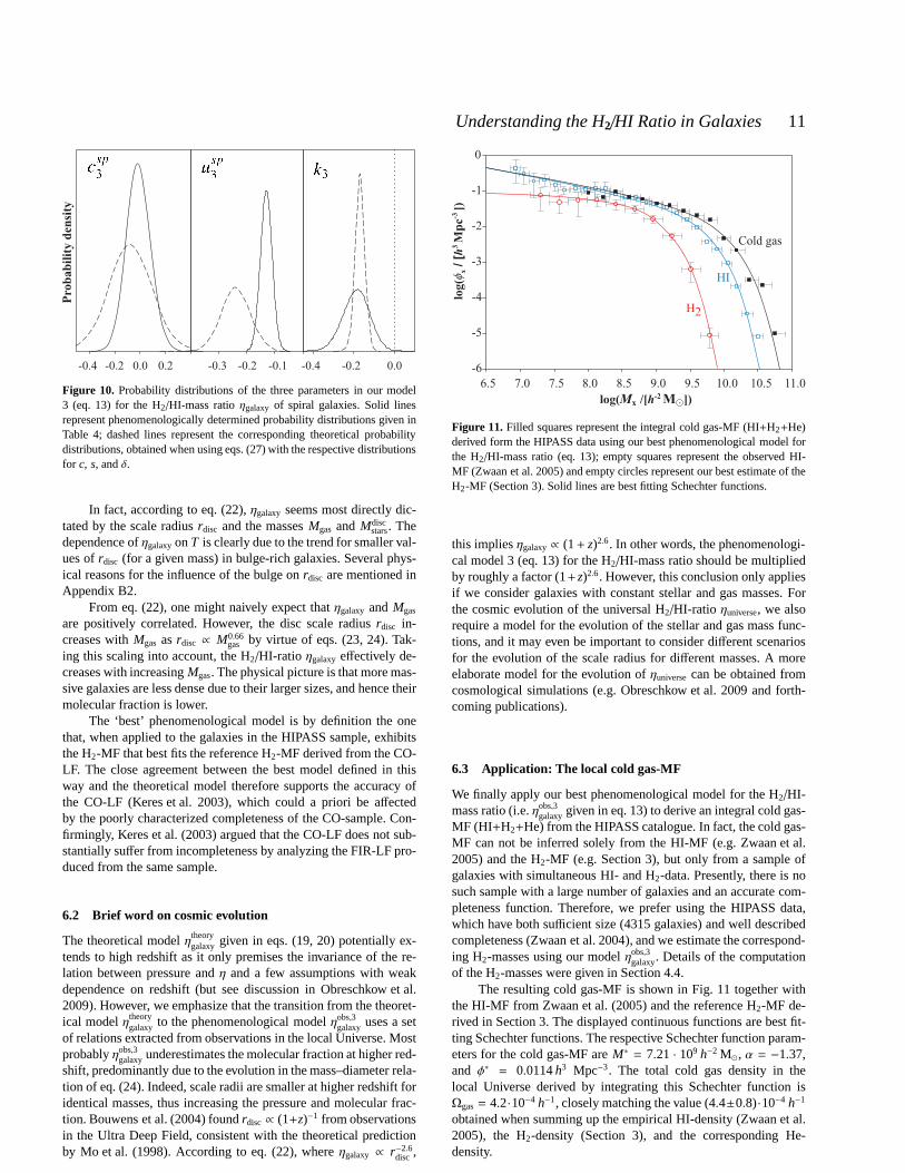
Figure 9. Relation betweenηtheorygalaxy(Mgas, 10) andMgas. The solid line rep-

resents the relation obtained from eq. (22), when expressing rdisc andMdiscstars

as functions ofMgas using eqs. (23, 24). The shaded zone represents the1-σ uncertainty implied by the uncertainties of the empirical parametersin eqs. (23, 24). The dashed line represents the best power-law fit for thedisplayed mass interval as given in eq. (26).

of the four parametersα1, α2, γ1, γ2. We approximate this relationby the power-law

log[

ηtheorygalaxy(Mgas,10)

]

= c + s · log

(

Mgas

109 h−2 M⊙

)

. (26)

The parameters minimizing the rms-deviation on the mass-intervallog(Mgas/[M⊙h−2]) = 7.5 − 10.5 arec = −1.79± 0.04 ands =−0.24± 0.05. The given uncertainties approximate the propagateduncertainties ofα1, α2, γ1, γ2.

The simplified theoretical model for the H2/HI-ratio given ineqs. (25, 26) exhibits exactly the formal structure of our best phe-nomenological model 3. Settingηtheory

galaxy(Mgas,T ) in eq. (25) equal to

ηobs,3galaxy(Mgas,T ) in eq. (13) for spiral galaxies, yields the following

mapping between the theoretical and empirical model-parameters,

csp3 = c − 1.6δ ,

usp3 = s , (27)

k3 = 0.16δ .

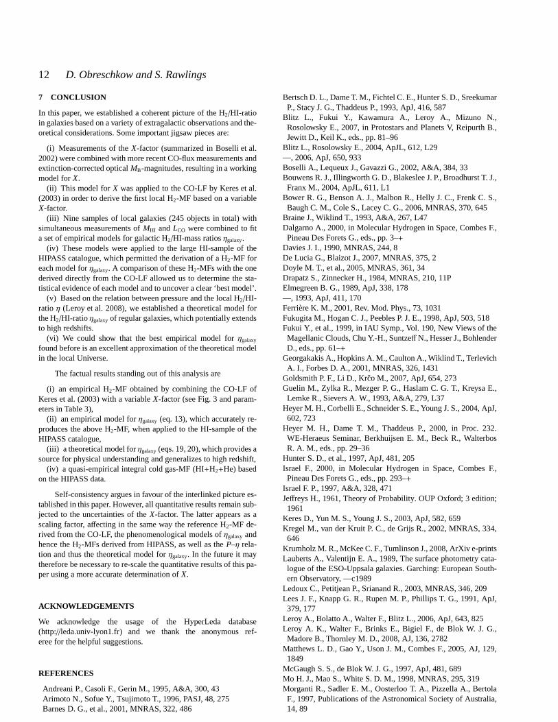
The probability distributions of the empirical model-parameters on the left hand side of eqs. (27) were derived in Section4 and their 1-σ uncertainties are given in Table 4. The correspond-ing probability distributions of the theoretical model-parameters onthe right hand side of eqs. (27) can be estimated from the Gaussianuncertainties given for the parametersc, s, δ. The empirical and the-oretical parameter distributions are compared in Fig. 10 and reveala surprising consistency.

6 DISCUSSION

6.1 Theoretical versus phenomenological model

The dependence ofηgalaxy on galaxy Hubble typeT and cold gasmassMgaswas first considered on a purely phenomenological level,and described by the empirical models in Section 4. The best em-pirical model for spiral galaxies could be quantitatively reproducedby the subsequently derived theoretical model for regular galaxiesin Section 5. Hence, the latter provides a tool for understanding thevariations ofηgalaxy.

c© 2008 RAS, MNRAS000, 1–20

Understanding the H2/HI Ratio in Galaxies 11

Pro

bab

ilit

y d

ensi

ty

0.0-0.1-0.2 -0.2-0.40.0 0.2-0.4 -0.2 -0.3

Figure 10. Probability distributions of the three parameters in our model3 (eq. 13) for the H2/HI-mass ratioηgalaxy of spiral galaxies. Solid linesrepresent phenomenologically determined probability distributions given inTable 4; dashed lines represent the corresponding theoretical probabilitydistributions, obtained when using eqs. (27) with the respective distributionsfor c, s, andδ.

In fact, according to eq. (22),ηgalaxy seems most directly dic-tated by the scale radiusrdisc and the massesMgas and Mdisc

stars. Thedependence ofηgalaxyonT is clearly due to the trend for smaller val-ues ofrdisc (for a given mass) in bulge-rich galaxies. Several phys-ical reasons for the influence of the bulge onrdisc are mentioned inAppendix B2.

From eq. (22), one might naively expect thatηgalaxy and Mgas

are positively correlated. However, the disc scale radiusrdisc in-creases withMgas asrdisc ∝ M0.66

gas by virtue of eqs. (23, 24). Tak-ing this scaling into account, the H2/HI-ratio ηgalaxy effectively de-creases with increasingMgas. The physical picture is that more mas-sive galaxies are less dense due to their larger sizes, and hence theirmolecular fraction is lower.

The ‘best’ phenomenological model is by definition the onethat, when applied to the galaxies in the HIPASS sample, exhibitsthe H2-MF that best fits the reference H2-MF derived from the CO-LF. The close agreement between the best model defined in thisway and the theoretical model therefore supports the accuracy ofthe CO-LF (Keres et al. 2003), which could a priori be affectedby the poorly characterized completeness of the CO-sample.Con-firmingly, Keres et al. (2003) argued that the CO-LF does not sub-stantially suffer from incompleteness by analyzing the FIR-LF pro-duced from the same sample.

6.2 Brief word on cosmic evolution

The theoretical modelηtheorygalaxy given in eqs. (19, 20) potentially ex-

tends to high redshift as it only premises the invariance of the re-lation between pressure andη and a few assumptions with weakdependence on redshift (but see discussion in Obreschkow etal.2009). However, we emphasize that the transition from the theoret-ical modelηtheory

galaxy to the phenomenological modelηobs,3galaxy uses a set

of relations extracted from observations in the local Universe. Mostprobablyηobs,3

galaxyunderestimates the molecular fraction at higher red-shift, predominantly due to the evolution in the mass–diameter rela-tion of eq. (24). Indeed, scale radii are smaller at higher redshift foridentical masses, thus increasing the pressure and molecular frac-tion. Bouwens et al. (2004) foundrdisc ∝ (1+z)−1 from observationsin the Ultra Deep Field, consistent with the theoretical predictionby Mo et al. (1998). According to eq. (22), whereηgalaxy ∝ r−2.6

disc ,

log( )Mx /[ ]h-2 M

-6

-5

-4

-3

-2

-1

0

6.5 7.0 7.5 8.0 8.5 9.0 9.5 10.0 10.5 11.0

H2

Cold gas

HI

log

(M

pc

])x/ [

-3h

3ff

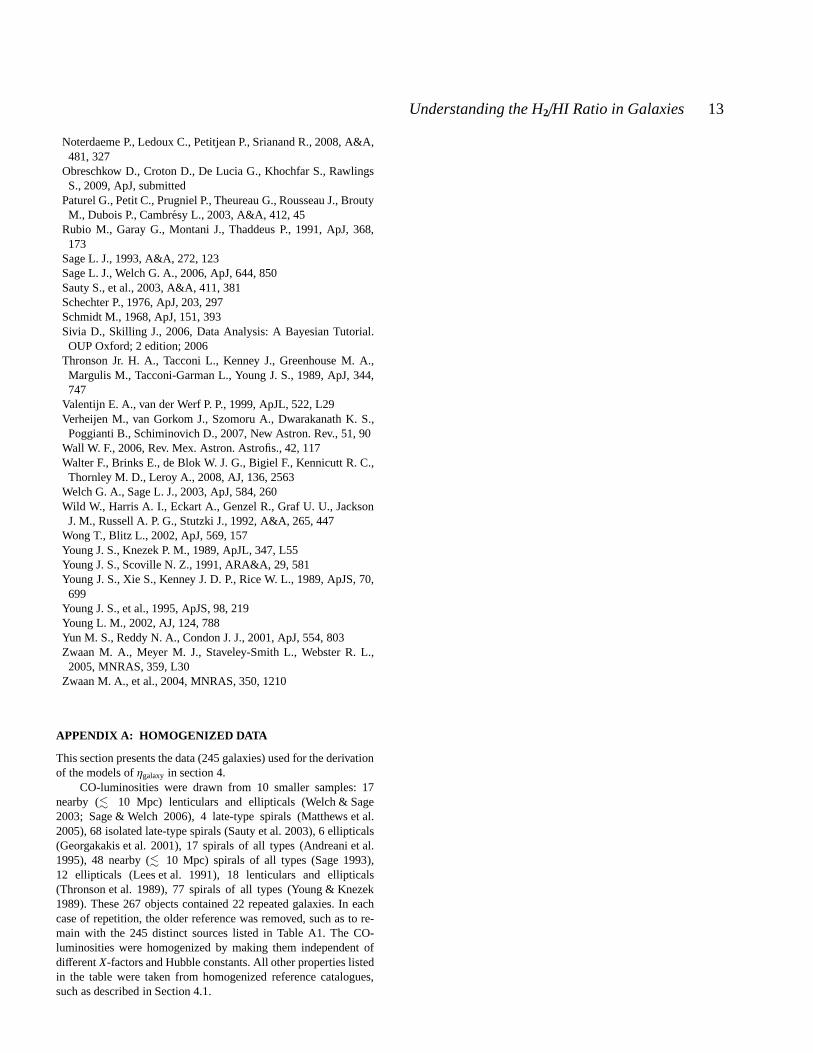
Figure 11. Filled squares represent the integral cold gas-MF (HI+H2+He)derived form the HIPASS data using our best phenomenological model forthe H2/HI-mass ratio (eq. 13); empty squares represent the observed HI-MF (Zwaan et al. 2005) and empty circles represent our best estimate of theH2-MF (Section 3). Solid lines are best fitting Schechter functions.

this impliesηgalaxy∝ (1+ z)2.6. In other words, the phenomenologi-cal model 3 (eq. 13) for the H2/HI-mass ratio should be multipliedby roughly a factor (1+ z)2.6. However, this conclusion only appliesif we consider galaxies with constant stellar and gas masses. Forthe cosmic evolution of the universal H2/HI-ratio ηuniverse, we alsorequire a model for the evolution of the stellar and gas mass func-tions, and it may even be important to consider different scenariosfor the evolution of the scale radius for different masses. A moreelaborate model for the evolution ofηuniversecan be obtained fromcosmological simulations (e.g. Obreschkow et al. 2009 and forth-coming publications).

6.3 Application: The local cold gas-MF

We finally apply our best phenomenological model for the H2/HI-mass ratio (i.e.ηobs,3

galaxy given in eq. 13) to derive an integral cold gas-MF (HI+H2+He) from the HIPASS catalogue. In fact, the cold gas-MF can not be inferred solely from the HI-MF (e.g. Zwaan et al.2005) and the H2-MF (e.g. Section 3), but only from a sample ofgalaxies with simultaneous HI- and H2-data. Presently, there is nosuch sample with a large number of galaxies and an accurate com-pleteness function. Therefore, we prefer using the HIPASS data,which have both sufficient size (4315 galaxies) and well describedcompleteness (Zwaan et al. 2004), and we estimate the correspond-ing H2-masses using our modelηobs,3

galaxy. Details of the computationof the H2-masses were given in Section 4.4.

The resulting cold gas-MF is shown in Fig. 11 together withthe HI-MF from Zwaan et al. (2005) and the reference H2-MF de-rived in Section 3. The displayed continuous functions are best fit-ting Schechter functions. The respective Schechter function param-eters for the cold gas-MF areM∗ = 7.21 · 109 h−2 M⊙, α = −1.37,and φ∗ = 0.0114h3 Mpc−3. The total cold gas density in thelocal Universe derived by integrating this Schechter function isΩgas= 4.2·10−4 h−1, closely matching the value (4.4±0.8)·10−4 h−1

obtained when summing up the empirical HI-density (Zwaan etal.2005), the H2-density (Section 3), and the corresponding He-density.

c© 2008 RAS, MNRAS000, 1–20

12 D. Obreschkow and S. Rawlings

7 CONCLUSION

In this paper, we established a coherent picture of the H2/HI-ratioin galaxies based on a variety of extragalactic observations and the-oretical considerations. Some important jigsaw pieces are:

(i) Measurements of theX-factor (summarized in Boselli et al.2002) were combined with more recent CO-flux measurements andextinction-corrected opticalMB-magnitudes, resulting in a workingmodel forX.

(ii) This model forX was applied to the CO-LF by Keres et al.(2003) in order to derive the first local H2-MF based on a variableX-factor.

(iii) Nine samples of local galaxies (245 objects in total) withsimultaneous measurements ofMHI andLCO were combined to fita set of empirical models for galactic H2/HI-mass ratiosηgalaxy.

(iv) These models were applied to the large HI-sample of theHIPASS catalogue, which permitted the derivation of a H2-MF foreach model forηgalaxy. A comparison of these H2-MFs with the onederived directly from the CO-LF allowed us to determine the sta-tistical evidence of each model and to uncover a clear ‘best model’.

(v) Based on the relation between pressure and the local H2/HI-ratio η (Leroy et al. 2008), we established a theoretical model forthe H2/HI-ratioηgalaxyof regular galaxies, which potentially extendsto high redshifts.

(vi) We could show that the best empirical model forηgalaxy

found before is an excellent approximation of the theoretical modelin the local Universe.

The factual results standing out of this analysis are

(i) an empirical H2-MF obtained by combining the CO-LF ofKeres et al. (2003) with a variableX-factor (see Fig. 3 and param-eters in Table 3),

(ii) an empirical model forηgalaxy (eq. 13), which accurately re-produces the above H2-MF, when applied to the HI-sample of theHIPASS catalogue,

(iii) a theoretical model forηgalaxy(eqs. 19, 20), which provides asource for physical understanding and generalizes to high redshift,

(iv) a quasi-empirical integral cold gas-MF (HI+H2+He) basedon the HIPASS data.

Self-consistency argues in favour of the interlinked picture es-tablished in this paper. However, all quantitative resultsremain sub-jected to the uncertainties of theX-factor. The latter appears as ascaling factor, affecting in the same way the reference H2-MF de-rived from the CO-LF, the phenomenological models ofηgalaxy andhence the H2-MFs derived from HIPASS, as well as theP–η rela-tion and thus the theoretical model forηgalaxy. In the future it maytherefore be necessary to re-scale the quantitative results of this pa-per using a more accurate determination ofX.

ACKNOWLEDGEMENTS

We acknowledge the usage of the HyperLeda database(http://leda.univ-lyon1.fr) and we thank the anonymous ref-eree for the helpful suggestions.

REFERENCES

Andreani P., Casoli F., Gerin M., 1995, A&A, 300, 43Arimoto N., Sofue Y., Tsujimoto T., 1996, PASJ, 48, 275Barnes D. G., et al., 2001, MNRAS, 322, 486

Bertsch D. L., Dame T. M., Fichtel C. E., Hunter S. D., SreekumarP., Stacy J. G., Thaddeus P., 1993, ApJ, 416, 587

Blitz L., Fukui Y., Kawamura A., Leroy A., Mizuno N.,Rosolowsky E., 2007, in Protostars and Planets V, Reipurth B.,Jewitt D., Keil K., eds., pp. 81–96

Blitz L., Rosolowsky E., 2004, ApJL, 612, L29—, 2006, ApJ, 650, 933Boselli A., Lequeux J., Gavazzi G., 2002, A&A, 384, 33Bouwens R. J., Illingworth G. D., Blakeslee J. P., Broadhurst T. J.,Franx M., 2004, ApJL, 611, L1

Bower R. G., Benson A. J., Malbon R., Helly J. C., Frenk C. S.,Baugh C. M., Cole S., Lacey C. G., 2006, MNRAS, 370, 645

Braine J., Wiklind T., 1993, A&A, 267, L47Dalgarno A., 2000, in Molecular Hydrogen in Space, Combes F.,Pineau Des Forets G., eds., pp. 3–+

Davies J. I., 1990, MNRAS, 244, 8De Lucia G., Blaizot J., 2007, MNRAS, 375, 2Doyle M. T., et al., 2005, MNRAS, 361, 34Drapatz S., Zinnecker H., 1984, MNRAS, 210, 11PElmegreen B. G., 1989, ApJ, 338, 178—, 1993, ApJ, 411, 170Ferriere K. M., 2001, Rev. Mod. Phys., 73, 1031Fukugita M., Hogan C. J., Peebles P. J. E., 1998, ApJ, 503, 518Fukui Y., et al., 1999, in IAU Symp., Vol. 190, New Views of theMagellanic Clouds, Chu Y.-H., SuntzeffN., Hesser J., BohlenderD., eds., pp. 61–+

Georgakakis A., Hopkins A. M., Caulton A., Wiklind T., TerlevichA. I., Forbes D. A., 2001, MNRAS, 326, 1431

Goldsmith P. F., Li D., Krco M., 2007, ApJ, 654, 273Guelin M., Zylka R., Mezger P. G., Haslam C. G. T., Kreysa E.,Lemke R., Sievers A. W., 1993, A&A, 279, L37

Heyer M. H., Corbelli E., Schneider S. E., Young J. S., 2004, ApJ,602, 723

Heyer M. H., Dame T. M., Thaddeus P., 2000, in Proc. 232.WE-Heraeus Seminar, Berkhuijsen E. M., Beck R., WalterbosR. A. M., eds., pp. 29–36

Hunter S. D., et al., 1997, ApJ, 481, 205Israel F., 2000, in Molecular Hydrogen in Space, Combes F.,Pineau Des Forets G., eds., pp. 293–+

Israel F. P., 1997, A&A, 328, 471Jeffreys H., 1961, Theory of Probability. OUP Oxford; 3 edition;1961

Keres D., Yun M. S., Young J. S., 2003, ApJ, 582, 659Kregel M., van der Kruit P. C., de Grijs R., 2002, MNRAS, 334,646

Krumholz M. R., McKee C. F., Tumlinson J., 2008, ArXiv e-printsLauberts A., Valentijn E. A., 1989, The surface photometry cata-logue of the ESO-Uppsala galaxies. Garching: European South-ern Observatory, —c1989

Ledoux C., Petitjean P., Srianand R., 2003, MNRAS, 346, 209Lees J. F., Knapp G. R., Rupen M. P., Phillips T. G., 1991, ApJ,379, 177

Leroy A., Bolatto A., Walter F., Blitz L., 2006, ApJ, 643, 825Leroy A. K., Walter F., Brinks E., Bigiel F., de Blok W. J. G.,Madore B., Thornley M. D., 2008, AJ, 136, 2782

Matthews L. D., Gao Y., Uson J. M., Combes F., 2005, AJ, 129,1849

McGaugh S. S., de Blok W. J. G., 1997, ApJ, 481, 689Mo H. J., Mao S., White S. D. M., 1998, MNRAS, 295, 319Morganti R., Sadler E. M., Oosterloo T. A., Pizzella A., BertolaF., 1997, Publications of the Astronomical Society of Australia,14, 89

c© 2008 RAS, MNRAS000, 1–20

Understanding the H2/HI Ratio in Galaxies 13

Noterdaeme P., Ledoux C., Petitjean P., Srianand R., 2008, A&A,481, 327

Obreschkow D., Croton D., De Lucia G., Khochfar S., RawlingsS., 2009, ApJ, submitted

Paturel G., Petit C., Prugniel P., Theureau G., Rousseau J.,BroutyM., Dubois P., Cambresy L., 2003, A&A, 412, 45

Rubio M., Garay G., Montani J., Thaddeus P., 1991, ApJ, 368,173

Sage L. J., 1993, A&A, 272, 123Sage L. J., Welch G. A., 2006, ApJ, 644, 850Sauty S., et al., 2003, A&A, 411, 381Schechter P., 1976, ApJ, 203, 297Schmidt M., 1968, ApJ, 151, 393Sivia D., Skilling J., 2006, Data Analysis: A Bayesian Tutorial.OUP Oxford; 2 edition; 2006

Thronson Jr. H. A., Tacconi L., Kenney J., Greenhouse M. A.,Margulis M., Tacconi-Garman L., Young J. S., 1989, ApJ, 344,747

Valentijn E. A., van der Werf P. P., 1999, ApJL, 522, L29Verheijen M., van Gorkom J., Szomoru A., Dwarakanath K. S.,Poggianti B., Schiminovich D., 2007, New Astron. Rev., 51, 90

Wall W. F., 2006, Rev. Mex. Astron. Astrofis., 42, 117Walter F., Brinks E., de Blok W. J. G., Bigiel F., Kennicutt R.C.,Thornley M. D., Leroy A., 2008, AJ, 136, 2563

Welch G. A., Sage L. J., 2003, ApJ, 584, 260Wild W., Harris A. I., Eckart A., Genzel R., Graf U. U., JacksonJ. M., Russell A. P. G., Stutzki J., 1992, A&A, 265, 447

Wong T., Blitz L., 2002, ApJ, 569, 157Young J. S., Knezek P. M., 1989, ApJL, 347, L55Young J. S., Scoville N. Z., 1991, ARA&A, 29, 581Young J. S., Xie S., Kenney J. D. P., Rice W. L., 1989, ApJS, 70,699

Young J. S., et al., 1995, ApJS, 98, 219Young L. M., 2002, AJ, 124, 788Yun M. S., Reddy N. A., Condon J. J., 2001, ApJ, 554, 803Zwaan M. A., Meyer M. J., Staveley-Smith L., Webster R. L.,2005, MNRAS, 359, L30

Zwaan M. A., et al., 2004, MNRAS, 350, 1210

APPENDIX A: HOMOGENIZED DATA

This section presents the data (245 galaxies) used for the derivationof the models ofηgalaxy in section 4.

CO-luminosities were drawn from 10 smaller samples: 17nearby (. 10 Mpc) lenticulars and ellipticals (Welch & Sage2003; Sage & Welch 2006), 4 late-type spirals (Matthews et al.2005), 68 isolated late-type spirals (Sauty et al. 2003), 6 ellipticals(Georgakakis et al. 2001), 17 spirals of all types (Andreaniet al.1995), 48 nearby (. 10 Mpc) spirals of all types (Sage 1993),12 ellipticals (Lees et al. 1991), 18 lenticulars and ellipticals(Thronson et al. 1989), 77 spirals of all types (Young & Knezek1989). These 267 objects contained 22 repeated galaxies. Ineachcase of repetition, the older reference was removed, such asto re-main with the 245 distinct sources listed in Table A1. The CO-luminosities were homogenized by making them independent ofdifferentX-factors and Hubble constants. All other properties listedin the table were taken from homogenized reference catalogues,such as described in Section 4.1.

c© 2008 RAS, MNRAS000, 1–20

14 D. Obreschkow and S. Rawlings

Table A1: Homogenized galaxy sample based on data drawn fromthe literature.T is the numerical Hubble type (see online help of the HyperLeda database),Dl the luminosity distance,MB is the extinction corrected absolute blue mag-nitude, andX is the variableX-factor derived fromMB (eq. 8) without addi-tion of Gaussian scatter. The references for H2-masses are: [1] Welch & Sage(2003); Sage & Welch (2006), [2] Matthews et al. (2005), [3] Sauty et al. (2003),[4] Georgakakis et al. (2001), [5] Andreani et al. (1995), [6] Sage (1993), [7]Lees et al. (1991), [8] Thronson et al. (1989), [9] Young & Knezek (1989).

Object T Dl / h−1 Mpc MB − 5 log h X log(MH2/X h−2 M⊙) Ref. H2 log(MHI/h−2 M⊙)

NGC 404 -2.8 1.7 -15.86 6.66 6.06 1 7.51NGC 2787 -1.1 9.5 -18.87 2.21 6.58 1 8.58NGC 3115 -2.8 6.4 -19.27 1.91 5.60 1 6.75NGC 3384 -2.7 9.2 -19.06 2.06 5.87 1 5.94NGC 3489 -1.3 7.7 -18.45 2.58 6.12 1 6.46NGC 3607 -3.1 10.3 -19.23 1.94 8.34 1 6.93NGC 3870 -2.0 9.9 -16.56 5.15 7.44 1 8.08NGC 3941 -2.0 11.0 -19.04 2.08 7.15 1 8.81NGC 4026 -1.8 12.1 -18.82 2.25 7.27 1 7.86NGC 4150 -2.1 6.8 -17.66 3.44 6.91 1 6.88NGC 4203 -2.7 12.7 -18.86 2.22 6.21 1 8.41NGC 4310 -1.0 10.8 -16.86 4.61 6.96 1 7.10NGC 4460 -0.9 7.3 -17.04 4.32 6.45 1 8.26NGC 4880 -1.5 14.8 -17.92 3.13 6.27 1 6.02NGC 7013 0.5 9.6 -18.79 2.28 7.30 1 8.70NGC 7077 -3.9 12.0 -16.13 6.03 6.09 1 7.60NGC 7457 -2.6 9.6 -18.29 2.73 5.85 1 5.88NGC 100 5.9 9.0 -17.61 3.51 5.91 2 8.87UGC 2082 5.9 7.7 -17.72 3.37 5.89 2 8.80UGC 3137 4.2 12.5 -17.05 4.30 6.20 2 9.11UGC 6667 6.0 12.1 -17.06 4.29 5.73 2 8.54UGC 5 3.9 74.4 -20.98 1.02 8.76 3 9.82NGC 7817 4.1 24.1 -20.42 1.25 8.44 3 9.30IC 1551 3.6 136.0 -22.17 0.66 8.94 3 9.34NGC 237 4.5 42.0 -19.81 1.57 8.53 3 9.75NGC 575 5.3 32.3 -19.10 2.03 8.04 3 9.18NGC 622 3.4 52.1 -19.93 1.50 8.24 3 9.54UGC 1167 5.9 43.6 -19.18 1.97 8.85 3 9.61UGC 1395 3.1 52.3 -19.90 1.51 8.43 3 9.25UGC 1587 3.7 57.4 -20.38 1.27 7.86 3 9.59UGC 1706 5.8 49.4 -19.82 1.56 7.96 3 9.17IC 302 4.1 59.6 -21.33 0.90 8.43 3 10.19IC 391 4.9 18.3 -18.91 2.18 7.46 3 8.89UGC 3420 3.1 54.5 -20.96 1.03 8.03 3 10.01UGC 3581 5.2 53.2 -20.30 1.31 8.24 3 9.56NGC 2344 4.4 11.3 -17.91 3.14 6.73 3 8.66UGC 3863 1.1 62.2 -20.53 1.20 8.32 3 9.30UGC 4684 7.2 24.9 -17.92 3.13 6.82 3 9.11NGC 2746 1.1 73.7 -20.65 1.15 8.65 3 9.64UGC 4781 5.9 14.4 -16.54 5.19 6.46 3 8.90UGC 5055 3.1 79.4 -20.19 1.36 8.79 3 10.02NGC 2900 5.9 54.3 -19.51 1.75 8.57 3 9.69NGC 2977 3.2 33.5 -19.95 1.49 8.31 3 8.83NGC 3049 2.5 15.0 -17.86 3.20 7.24 3 8.86IC 651 8.2 45.2 -20.37 1.28 8.54 3 9.53NGC 3526 5.2 14.5 -18.68 2.37 7.73 3 8.64UGC 6568 8.2 60.8 -19.86 1.54 8.12 3 9.14UGC 6769 3.0 88.2 -20.66 1.15 9.10 3 9.96UGC 6780 6.4 17.3 -16.79 4.73 7.29 3 9.28UGC 6879 7.1 24.1 -18.78 2.28 7.82 3 8.83UGC 6903 5.9 19.3 -17.69 3.40 7.46 3 9.07

c© 2008 RAS, MNRAS000, 1–20

Understanding the H2/HI Ratio in Galaxies 15

Object T Dl /[ h−1 Mpc] MB − 5 log h X log(MH2/[X h−2 M⊙]) Ref. H2 log(MHI/[h−2 M⊙])

NGC 4348 4.1 20.3 -19.49 1.76 8.10 3 9.01NGC 4617 3.1 49.6 -20.70 1.13 8.56 3 9.90NGC 4635 6.5 10.9 -17.28 3.96 6.73 3 8.23NGC 5377 1.1 20.6 -19.83 1.55 7.81 3 8.91NGC 5375 2.4 26.0 -19.54 1.73 7.60 3 9.24NGC 5584 5.9 17.1 -19.06 2.06 7.22 3 9.27NGC 5690 5.4 18.4 -19.88 1.53 8.15 3 9.33NGC 5768 5.3 20.3 -18.74 2.32 7.90 3 9.11NGC 5772 3.1 52.3 -20.41 1.26 8.25 3 9.49NGC 5913 1.3 20.8 -19.00 2.11 8.22 3 8.44NGC 6012 1.9 20.1 -19.00 2.11 7.73 3 9.26IC 1231 5.8 55.9 -20.71 1.13 8.04 3 9.14UGC 10699 4.4 65.5 -20.19 1.36 8.60 3 9.11UGC 10743 1.1 27.2 -18.75 2.31 7.52 3 8.78NGC 6347 3.1 64.3 -20.46 1.23 8.57 3 9.48UGC 10862 5.3 18.2 -17.81 3.26 7.21 3 9.07NGC 6389 3.6 33.1 -20.37 1.28 8.30 3 9.93UGC 11058 3.2 50.6 -20.48 1.22 8.51 3 9.40NGC 6643 5.2 17.8 -20.31 1.30 8.35 3 9.27NGC 6711 4.0 50.1 -20.18 1.37 8.77 3 9.14UGC 11635 3.7 51.8 -21.05 0.99 8.95 3 9.88UGC 11723 3.1 50.1 -19.87 1.53 8.48 3 9.57NGC 7056 3.6 55.8 -20.53 1.20 8.67 3 9.11NGC 7156 5.9 40.8 -20.12 1.40 8.43 3 9.32UGC 11871 3.1 82.9 -20.38 1.27 9.22 3 9.43NGC 7328 2.1 29.2 -19.31 1.88 8.34 3 9.45NGC 7428 1.1 31.0 -18.85 2.23 7.72 3 9.44UGC 12304 5.2 35.3 -19.40 1.82 8.01 3 8.88UGC 12372 4.0 57.7 -19.94 1.49 8.65 3 9.49NGC 7514 4.3 51.1 -20.62 1.16 8.18 3 9.16UGC 12474 1.1 53.5 -20.53 1.20 8.80 3 8.87NGC 7664 5.1 36.3 -20.03 1.44 8.51 3 9.91UGC 12646 3.0 83.7 -20.84 1.07 8.68 3 9.70NGC 7712 1.6 31.9 -18.94 2.15 7.84 3 9.10IC 1508 7.2 43.8 -20.07 1.42 8.45 3 9.75UGC 12776 3.0 51.8 -19.88 1.53 8.31 3 9.99IC 5355 5.7 50.8 -19.56 1.72 8.26 3 9.05UGC 12840 -1.8 71.3 -20.27 1.32 7.97 3 9.43NGC 2623 2.0 57.2 -20.59 1.18 9.02 4 9.01NGC 2865 -4.1 26.0 -20.01 1.46 7.35 4 8.79NGC 3921 0.0 61.9 -21.00 1.01 8.82 4 9.46NGC 4649 -4.6 12.1 -20.70 1.13 7.15 4 8.35NGC 7252 -2.1 47.0 -20.73 1.12 8.83 4 9.29NGC 7727 1.1 17.9 -19.98 1.47 7.27 4 8.45NGC 142 3.1 81.4 -20.46 1.23 9.36 5 9.43IC 1553 5.4 28.0 -18.75 2.31 7.69 5 9.10ESO 473-27 4.4 193.6 -21.12 0.97 9.78 5 9.75NGC 232 1.1 66.7 -19.82 1.56 9.50 5 9.21ESO 475-16 2.1 70.7 -20.44 1.24 9.01 5 9.74NGC 578 5.0 14.8 -19.73 1.61 7.97 5 9.52ESO 478-6 4.1 52.6 -20.64 1.16 8.96 5 9.23NGC 1187 5.0 12.2 -19.39 1.83 8.69 5 9.33NGC 1306 2.8 12.7 -16.85 4.63 7.34 5 8.64NGC 1385 5.9 13.1 -19.56 1.72 8.59 5 9.07ESO 549-23 1.2 40.8 -19.42 1.81 8.45 5 8.88ESO 483-12 0.3 41.0 -19.18 1.97 8.27 5 8.83NGC 1591 1.9 39.5 -19.65 1.66 8.51 5 9.04NGC 7115 3.4 34.1 -19.53 1.73 8.26 5 9.52NGC 7225 -0.5 47.9 -20.09 1.41 9.29 5 9.07NGC 7314 4.0 13.2 -19.71 1.62 8.05 5 9.24

c© 2008 RAS, MNRAS000, 1–20

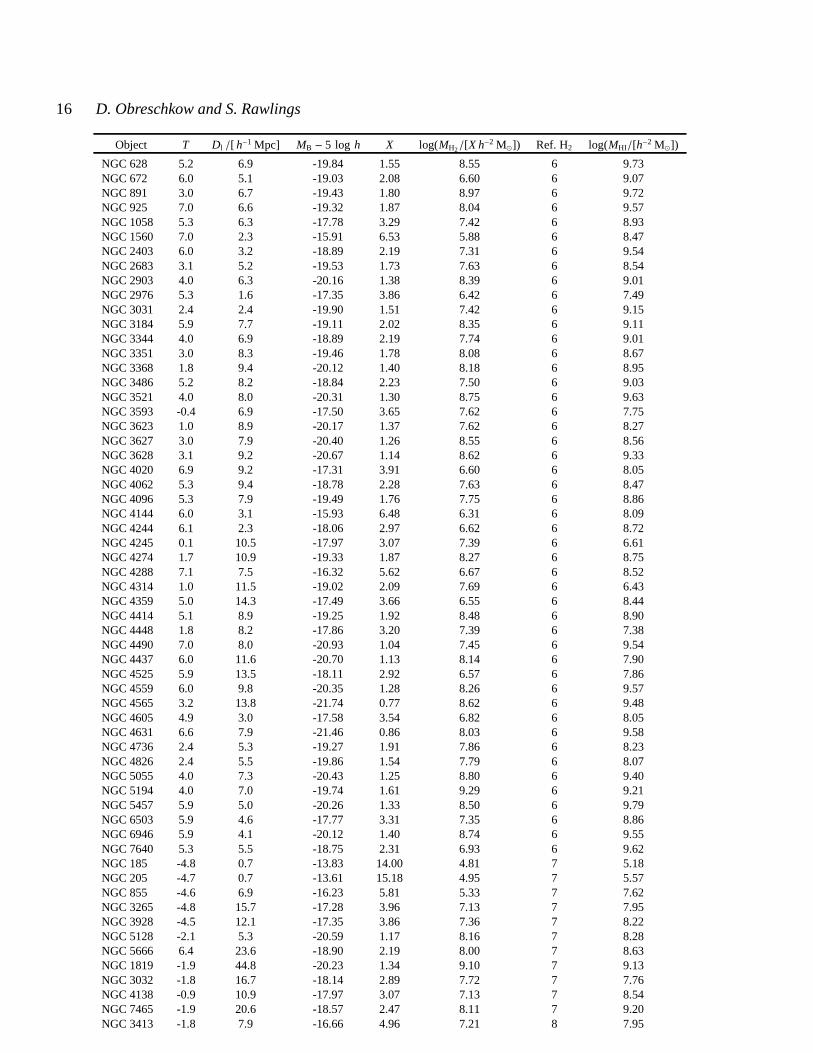
16 D. Obreschkow and S. Rawlings

Object T Dl /[ h−1 Mpc] MB − 5 log h X log(MH2/[X h−2 M⊙]) Ref. H2 log(MHI/[h−2 M⊙])

NGC 628 5.2 6.9 -19.84 1.55 8.55 6 9.73NGC 672 6.0 5.1 -19.03 2.08 6.60 6 9.07NGC 891 3.0 6.7 -19.43 1.80 8.97 6 9.72NGC 925 7.0 6.6 -19.32 1.87 8.04 6 9.57NGC 1058 5.3 6.3 -17.78 3.29 7.42 6 8.93NGC 1560 7.0 2.3 -15.91 6.53 5.88 6 8.47NGC 2403 6.0 3.2 -18.89 2.19 7.31 6 9.54NGC 2683 3.1 5.2 -19.53 1.73 7.63 6 8.54NGC 2903 4.0 6.3 -20.16 1.38 8.39 6 9.01NGC 2976 5.3 1.6 -17.35 3.86 6.42 6 7.49NGC 3031 2.4 2.4 -19.90 1.51 7.42 6 9.15NGC 3184 5.9 7.7 -19.11 2.02 8.35 6 9.11NGC 3344 4.0 6.9 -18.89 2.19 7.74 6 9.01NGC 3351 3.0 8.3 -19.46 1.78 8.08 6 8.67NGC 3368 1.8 9.4 -20.12 1.40 8.18 6 8.95NGC 3486 5.2 8.2 -18.84 2.23 7.50 6 9.03NGC 3521 4.0 8.0 -20.31 1.30 8.75 6 9.63NGC 3593 -0.4 6.9 -17.50 3.65 7.62 6 7.75NGC 3623 1.0 8.9 -20.17 1.37 7.62 6 8.27NGC 3627 3.0 7.9 -20.40 1.26 8.55 6 8.56NGC 3628 3.1 9.2 -20.67 1.14 8.62 6 9.33NGC 4020 6.9 9.2 -17.31 3.91 6.60 6 8.05NGC 4062 5.3 9.4 -18.78 2.28 7.63 6 8.47NGC 4096 5.3 7.9 -19.49 1.76 7.75 6 8.86NGC 4144 6.0 3.1 -15.93 6.48 6.31 6 8.09NGC 4244 6.1 2.3 -18.06 2.97 6.62 6 8.72NGC 4245 0.1 10.5 -17.97 3.07 7.39 6 6.61NGC 4274 1.7 10.9 -19.33 1.87 8.27 6 8.75NGC 4288 7.1 7.5 -16.32 5.62 6.67 6 8.52NGC 4314 1.0 11.5 -19.02 2.09 7.69 6 6.43NGC 4359 5.0 14.3 -17.49 3.66 6.55 6 8.44NGC 4414 5.1 8.9 -19.25 1.92 8.48 6 8.90NGC 4448 1.8 8.2 -17.86 3.20 7.39 6 7.38NGC 4490 7.0 8.0 -20.93 1.04 7.45 6 9.54NGC 4437 6.0 11.6 -20.70 1.13 8.14 6 7.90NGC 4525 5.9 13.5 -18.11 2.92 6.57 6 7.86NGC 4559 6.0 9.8 -20.35 1.28 8.26 6 9.57NGC 4565 3.2 13.8 -21.74 0.77 8.62 6 9.48NGC 4605 4.9 3.0 -17.58 3.54 6.82 6 8.05NGC 4631 6.6 7.9 -21.46 0.86 8.03 6 9.58NGC 4736 2.4 5.3 -19.27 1.91 7.86 6 8.23NGC 4826 2.4 5.5 -19.86 1.54 7.79 6 8.07NGC 5055 4.0 7.3 -20.43 1.25 8.80 6 9.40NGC 5194 4.0 7.0 -19.74 1.61 9.29 6 9.21NGC 5457 5.9 5.0 -20.26 1.33 8.50 6 9.79NGC 6503 5.9 4.6 -17.77 3.31 7.35 6 8.86NGC 6946 5.9 4.1 -20.12 1.40 8.74 6 9.55NGC 7640 5.3 5.5 -18.75 2.31 6.93 6 9.62NGC 185 -4.8 0.7 -13.83 14.00 4.81 7 5.18NGC 205 -4.7 0.7 -13.61 15.18 4.95 7 5.57NGC 855 -4.6 6.9 -16.23 5.81 5.33 7 7.62NGC 3265 -4.8 15.7 -17.28 3.96 7.13 7 7.95NGC 3928 -4.5 12.1 -17.35 3.86 7.36 7 8.22NGC 5128 -2.1 5.3 -20.59 1.17 8.16 7 8.28NGC 5666 6.4 23.6 -18.90 2.19 8.00 7 8.63NGC 1819 -1.9 44.8 -20.23 1.34 9.10 7 9.13NGC 3032 -1.8 16.7 -18.14 2.89 7.72 7 7.76NGC 4138 -0.9 10.9 -17.97 3.07 7.13 7 8.54NGC 7465 -1.9 20.6 -18.57 2.47 8.11 7 9.20NGC 3413 -1.8 7.9 -16.66 4.96 7.21 8 7.95

c© 2008 RAS, MNRAS000, 1–20

Understanding the H2/HI Ratio in Galaxies 17

Object T Dl /[ h−1 Mpc] MB − 5 log h X log(MH2/[X h−2 M⊙]) Ref. H2 log(MHI/[h−2 M⊙])

NGC 5866 -1.2 9.5 -19.23 1.94 7.81 8 8.15NGC 4710 -0.8 13.8 -19.02 2.09 8.25 8 7.20NGC 4459 -1.4 13.3 -19.37 1.84 8.30 8 6.70NGC 4526 -1.9 6.7 -18.63 2.41 8.30 8 7.05NGC 693 0.1 15.5 -18.08 2.95 7.53 8 8.74NGC 2685 -1.1 11.0 -18.32 2.70 7.45 8 8.79NGC 2273 1.0 20.7 -19.47 1.77 8.26 8 8.90NGC 3611 1.1 16.1 -18.67 2.38 8.42 8 8.75NGC 4457 0.4 9.4 -18.31 2.71 8.63 8 8.27NGC 4383 1.0 18.3 -19.01 2.10 7.91 8 9.15NGC 7625 1.2 17.2 -18.38 2.64 8.56 8 8.98NGC 23 1.2 47.4 -20.84 1.07 9.30 9 9.69NGC 253 5.1 1.7 -20.19 1.36 8.32 9 9.04NGC 520 0.8 21.5 -19.90 1.51 9.35 9 9.50NGC 828 1.0 55.9 -20.95 1.03 9.75 9 9.80NGC 834 3.9 48.1 -20.32 1.30 9.13 9 9.47NGC 864 5.1 15.4 -19.80 1.57 8.49 9 9.78NGC 877 4.8 39.7 -21.15 0.96 9.34 9 10.08NGC 1055 3.2 9.3 -18.97 2.13 9.37 9 9.39IC 342 5.9 2.3 -19.85 1.54 8.70 9 9.68NGC 1530 3.1 27.5 -20.70 1.13 9.10 9 9.76NGC 1569 9.6 2.4 -15.94 6.46 5.89 9 8.09NGC 1614 4.9 47.2 -20.64 1.16 9.36 9 9.28NGC 2146 2.3 11.6 -20.34 1.29 9.04 9 9.50NGC 2339 4.0 22.9 -20.02 1.45 9.27 9 9.45NGC 2276 5.4 27.2 -20.80 1.09 9.31 9 9.50NGC 2532 5.2 54.5 -21.00 1.01 9.10 9 9.92NGC 2633 3.0 24.5 -19.47 1.77 8.83 9 9.41NGC 2775 1.7 13.5 -19.83 1.55 8.30 9 8.16NGC 2841 3.0 8.3 -20.07 1.42 8.61 9 9.20NGC 3034 8.0 1.7 -17.30 3.93 8.16 9 8.54NGC 3079 6.6 13.5 -20.68 1.14 9.16 9 9.57NGC 3147 3.9 31.1 -21.43 0.86 9.65 9 9.52NGC 3221 5.6 42.5 -19.86 1.54 9.24 9 9.81NGC 3310 4.0 12.2 -19.26 1.92 7.81 9 9.33NGC 3437 5.2 13.8 -19.03 2.08 7.91 9 9.03NGC 3504 2.1 16.8 -19.68 1.64 8.50 9 8.37NGC 3556 6.0 9.3 -19.89 1.52 8.37 9 9.35NGC 3893 5.1 12.0 -20.13 1.39 8.35 9 9.29NGC 4192 2.5 10.0 -20.83 1.08 8.57 9 9.33NGC 4194 9.7 27.3 -19.87 1.53 8.61 9 8.96NGC 4254 5.2 25.2 -21.82 0.75 9.07 9 9.39NGC 4303 4.0 16.2 -21.05 0.99 8.95 9 9.38NGC 4321 4.0 16.8 -21.29 0.91 9.12 9 9.06NGC 4388 2.8 26.2 -21.16 0.95 7.96 9 8.33NGC 4394 2.9 10.3 -18.65 2.39 8.04 9 8.22NGC 4402 3.3 10.0 -17.18 4.09 8.39 9 8.23NGC 4419 1.1 10.0 -18.43 2.60 8.56 9 7.62NGC 4424 1.2 5.1 -15.75 6.91 7.34 9 7.89NGC 4438 0.7 10.0 -19.99 1.47 7.92 9 8.26NGC 4449 9.8 2.6 -16.83 4.66 6.60 9 9.10NGC 4450 2.3 20.7 -21.10 0.98 8.25 9 7.95NGC 4501 3.4 23.9 -22.33 0.62 8.94 9 8.91NGC 4527 4.0 17.9 -20.75 1.11 8.85 9 9.35NGC 4535 5.0 20.3 -21.18 0.95 8.79 9 9.41NGC 4536 4.2 18.6 -21.02 1.01 8.46 9 9.23NGC 4548 3.1 6.0 -20.01 1.46 8.33 9 8.68NGC 4569 2.4 10.0 -20.33 1.29 8.77 9 8.32NGC 4571 6.3 10.0 -17.53 3.60 8.17 9 8.49NGC 4579 2.8 16.1 -20.91 1.05 8.55 9 8.38

c© 2008 RAS, MNRAS000, 1–20

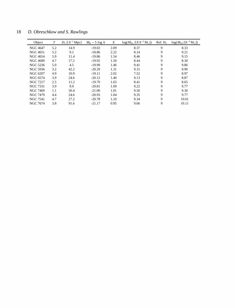
18 D. Obreschkow and S. Rawlings

Object T Dl /[ h−1 Mpc] MB − 5 log h X log(MH2/[X h−2 M⊙]) Ref. H2 log(MHI/[h−2 M⊙])

NGC 4647 5.2 14.9 -19.02 2.09 8.37 9 8.33NGC 4651 5.2 9.1 -18.86 2.22 8.14 9 9.21NGC 4654 5.9 11.4 -19.86 1.54 8.46 9 9.15NGC 4689 4.7 17.2 -19.92 1.50 8.44 9 8.30NGC 5236 5.0 4.5 -19.99 1.46 9.41 9 9.86NGC 5936 3.2 42.2 -20.29 1.31 9.15 9 8.90NGC 6207 4.9 10.9 -19.11 2.02 7.52 9 8.97NGC 6574 3.9 24.6 -20.12 1.40 9.13 9 8.87NGC 7217 2.5 11.2 -19.70 1.63 8.41 9 8.65NGC 7331 3.9 9.9 -20.81 1.09 9.22 9 9.77NGC 7469 1.1 50.4 -21.00 1.01 9.50 9 9.30NGC 7479 4.4 24.6 -20.93 1.04 9.35 9 9.77NGC 7541 4.7 27.2 -20.78 1.10 9.34 9 10.01NGC 7674 3.8 91.6 -21.17 0.95 9.66 9 10.11

c© 2008 RAS, MNRAS000, 1–20

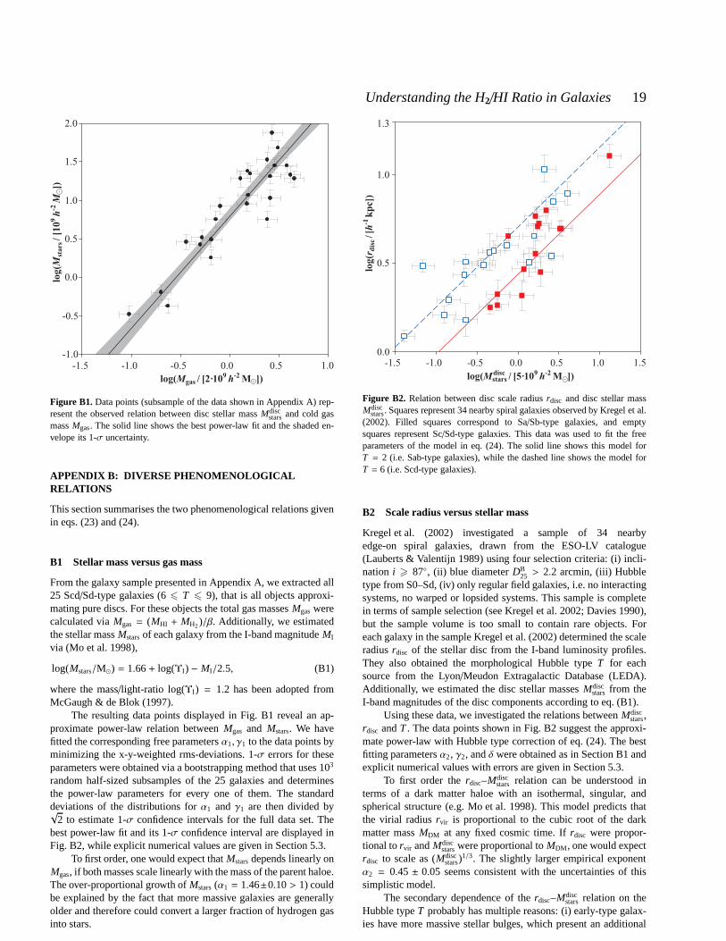
Understanding the H2/HI Ratio in Galaxies 19

log( / [2 10 ])Mgas9 -2

· h M

-1.0

-0.5

0.0

0.5

1.0

1.5

2.0

-1.5 -1.0 -0.5 0.0 0.5 1.0

log(

/ [1

0])

Mst

ars

9-2

hM

Figure B1. Data points (subsample of the data shown in Appendix A) rep-resent the observed relation between disc stellar massMdisc

stars and cold gasmassMgas. The solid line shows the best power-law fit and the shaded en-velope its 1-σ uncertainty.

APPENDIX B: DIVERSE PHENOMENOLOGICALRELATIONS

This section summarises the two phenomenological relations givenin eqs. (23) and (24).

B1 Stellar mass versus gas mass

From the galaxy sample presented in Appendix A, we extractedall25 Scd/Sd-type galaxies (66 T 6 9), that is all objects approxi-mating pure discs. For these objects the total gas massesMgaswerecalculated viaMgas = (MHI + MH2)/β. Additionally, we estimatedthe stellar massMstarsof each galaxy from the I-band magnitudeMI

via (Mo et al. 1998),

log(Mstars/M⊙) = 1.66+ log(ΥI) − MI/2.5, (B1)

where the mass/light-ratio log(ΥI) = 1.2 has been adopted fromMcGaugh & de Blok (1997).

The resulting data points displayed in Fig. B1 reveal an ap-proximate power-law relation betweenMgas and Mstars. We havefitted the corresponding free parametersα1, γ1 to the data points byminimizing the x-y-weighted rms-deviations. 1-σ errors for theseparameters were obtained via a bootstrapping method that uses 103

random half-sized subsamples of the 25 galaxies and determinesthe power-law parameters for every one of them. The standarddeviations of the distributions forα1 and γ1 are then divided by√

2 to estimate 1-σ confidence intervals for the full data set. Thebest power-law fit and its 1-σ confidence interval are displayed inFig. B2, while explicit numerical values are given in Section 5.3.

To first order, one would expect thatMstarsdepends linearly onMgas, if both masses scale linearly with the mass of the parent haloe.The over-proportional growth ofMstars(α1 = 1.46±0.10> 1) couldbe explained by the fact that more massive galaxies are generallyolder and therefore could convert a larger fraction of hydrogen gasinto stars.

0.0

0.5

1.0

-1.5 -1.0 -0.5 0.0 0.5 1.0 1.5lo

g(

)r

dis

c/[

kp

c]h

-1

log( / [5 10 ])Mstars9 -2

· h M

1.3

disc

Figure B2. Relation between disc scale radiusrdisc and disc stellar massMdisc

stars. Squares represent 34 nearby spiral galaxies observed by Kregel et al.(2002). Filled squares correspond to Sa/Sb-type galaxies, and emptysquares represent Sc/Sd-type galaxies. This data was used to fit the freeparameters of the model in eq. (24). The solid line shows thismodel forT = 2 (i.e. Sab-type galaxies), while the dashed line shows the model forT = 6 (i.e. Scd-type galaxies).

B2 Scale radius versus stellar mass

Kregel et al. (2002) investigated a sample of 34 nearbyedge-on spiral galaxies, drawn from the ESO-LV catalogue(Lauberts & Valentijn 1989) using four selection criteria:(i) incli-nation i > 87, (ii) blue diameterDB

25 > 2.2 arcmin, (iii) Hubbletype from S0–Sd, (iv) only regular field galaxies, i.e. no interactingsystems, no warped or lopsided systems. This sample is completein terms of sample selection (see Kregel et al. 2002; Davies 1990),but the sample volume is too small to contain rare objects. Foreach galaxy in the sample Kregel et al. (2002) determined thescaleradiusrdisc of the stellar disc from the I-band luminosity profiles.They also obtained the morphological Hubble typeT for eachsource from the Lyon/Meudon Extragalactic Database (LEDA).Additionally, we estimated the disc stellar massesMdisc

stars from theI-band magnitudes of the disc components according to eq. (B1).

Using these data, we investigated the relations betweenMdiscstars,

rdisc andT . The data points shown in Fig. B2 suggest the approxi-mate power-law with Hubble type correction of eq. (24). The bestfitting parametersα2, γ2, andδ were obtained as in Section B1 andexplicit numerical values with errors are given in Section 5.3.

To first order therdisc–Mdiscstars relation can be understood in

terms of a dark matter haloe with an isothermal, singular, andspherical structure (e.g. Mo et al. 1998). This model predicts thatthe virial radiusrvir is proportional to the cubic root of the darkmatter massMDM at any fixed cosmic time. Ifrdisc were propor-tional torvir andMdisc

starswere proportional toMDM , one would expectrdisc to scale as (Mdisc

stars)1/3. The slightly larger empirical exponent

α2 = 0.45 ± 0.05 seems consistent with the uncertainties of thissimplistic model.

The secondary dependence of therdisc–Mdiscstars relation on the

Hubble typeT probably has multiple reasons: (i) early-type galax-ies have more massive stellar bulges, which present an additional

c© 2008 RAS, MNRAS000, 1–20

20 D. Obreschkow and S. Rawlings

central potential that contracts the disc; (ii) bulges often form fromdisc instabilities, occurring preferably in systems with relativelylow angular momentum, and hence early-type galaxies are biasedtowards smaller angular momenta and smaller scale radii; (iii)larger bulges, such as the ones of lenticular and ellipticalgalaxies,often arise from galaxy mergers, which tend to reduce the specificangular momenta and scale radii (see also Obreschkow et al. 2009).

c© 2008 RAS, MNRAS000, 1–20