
Understanding the Middle Miocene Climatic Optimum ...
53
Understanding the Middle Miocene Climatic Optimum: Evaluation of Deuterium Values (δD) Related to Precipitation and Temperature BY: Colin Gannon ADVISORS • Hong Yang _________________________________________________________________________________________ Submitted in partial fulfillment of the requirements for graduation with honors in the Bryant University Honors Program APRIL 2013
Transcript of Understanding the Middle Miocene Climatic Optimum ...
Understanding the Middle Miocene Climatic Optimum: Evaluation of Deuterium Values (δD) Related to Precipitation and Temperature BY: Colin Gannon
ADVISORS • Hong Yang _________________________________________________________________________________________ Submitted in partial fulfillment of the requirements for graduation with honors in the Bryant University Honors Program APRIL 2013
Understanding the Middle Miocene Climatic Optimum Senior Capstone Project for Colin Gannon
-2-
Table of Contents
Foreword ......................................................................................................................................... 3
Reading this Capstone ................................................................................................................. 3
Background ................................................................................................................................. 3
About Our Research .................................................................................................................... 5
Introduction ..................................................................................................................................... 8
Characteristics of the Middle Miocene Climatic Optimum ........................................................ 9
Mehtods......................................................................................................................................... 10
Sample Selection and Location ................................................................................................. 10
Sample Preparation and Measurements .................................................................................... 11
Data Analysis .............................................................................................................................. 13
Model Description ..................................................................................................................... 16
Adjusting Data Points ............................................................................................................ 18
Adjusted Model Description .................................................................................................. 22
Discussion ..................................................................................................................................... 26
Conclusions ................................................................................................................................... 31
Acknowledgements ....................................................................................................................... 32
References ..................................................................................................................................... 33
Afterword ...................................................................................................................................... 38
Appendices .................................................................................................................................... 40
Appendix A: Glossary ............................................................................................................... 41
Appendix B: Chromatographs ................................................................................................... 47
Appendix C: Geologic Time Periods ........................................................................................ 50
Appendix D: Model Details ...................................................................................................... 51
Understanding the Middle Miocene Climatic Optimum Senior Capstone Project for Colin Gannon
-3-
Understanding the Middle Miocene Climatic Optimum: Evaluation of
Deuterium Values (D) Related to Temperature and Precipitation
Colin Gannon1, Brian Blais
1,2, Qin Leng
1, Robert Patalano
1, Hong Yang
1
1Laboratory for Terrestrial Environments, Department of Science and Technology, College of Arts and Science, Bryant
University, Smithfield, RI, USA; 2Institute for Brain and Neural Systems, Brown University, Providence, RI, USA
FOREWORD
Reading this Capstone
This capstone is organized in the form of a scientific journal article and has been written with
intent to submit as a publication. The Abstract, Introduction, Methods, Data Analysis, Discussion,
and Conclusion sections thoroughly outline the process of preparing samples for evaluation, and
subsequent interpretations of the relationship between the data and the Middle Miocene Climatic
Optimum.
This Foreword, along with the Afterword and Appendices following the manuscript, have all
been included for the benefit of this Honors Capstone to provide a background of the overall
concepts of this research. For any unfamiliar vocabulary, please refer to Appendix A, which
contains a full glossary of the technical terms used throughout this manuscript.
Background
Understanding and forecasting climate, even with modern day technology and supercomputers,
is a dauntingly complex task. The climate of any given location is inextricably connected to
myriad factors, susceptible to change with any fluctuation in a multitude of variables. To
illustrate climate dynamics, it is best to begin by breaking down the Earth into “spheres.” These
include the atmosphere, biosphere, hydrosphere, and geosphere, each having many sub-divisions
themselves. These spheres have been evaluated by the scientific community thoroughly, their
physical features identified, helping us to understand the dynamics of each. These spheres are
deeply interconnected, and it is when these linkages are studied that we can begin to elucidate
climate on a larger scale.
Understanding the Middle Miocene Climatic Optimum Senior Capstone Project for Colin Gannon
-4-
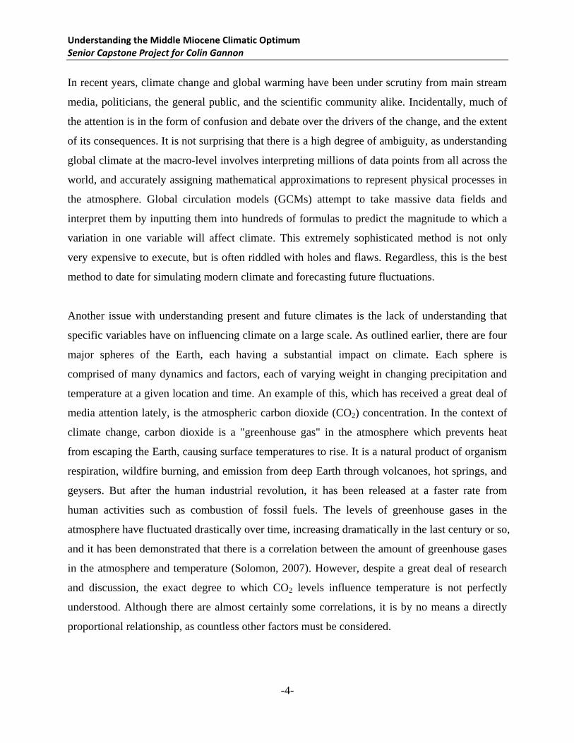
In recent years, climate change and global warming have been under scrutiny from main stream
media, politicians, the general public, and the scientific community alike. Incidentally, much of
the attention is in the form of confusion and debate over the drivers of the change, and the extent
of its consequences. It is not surprising that there is a high degree of ambiguity, as understanding
global climate at the macro-level involves interpreting millions of data points from all across the
world, and accurately assigning mathematical approximations to represent physical processes in
the atmosphere. Global circulation models (GCMs) attempt to take massive data fields and
interpret them by inputting them into hundreds of formulas to predict the magnitude to which a
variation in one variable will affect climate. This extremely sophisticated method is not only
very expensive to execute, but is often riddled with holes and flaws. Regardless, this is the best
method to date for simulating modern climate and forecasting future fluctuations.
Another issue with understanding present and future climates is the lack of understanding that
specific variables have on influencing climate on a large scale. As outlined earlier, there are four
major spheres of the Earth, each having a substantial impact on climate. Each sphere is
comprised of many dynamics and factors, each of varying weight in changing precipitation and
temperature at a given location and time. An example of this, which has received a great deal of
media attention lately, is the atmospheric carbon dioxide (CO2) concentration. In the context of
climate change, carbon dioxide is a "greenhouse gas" in the atmosphere which prevents heat
from escaping the Earth, causing surface temperatures to rise. It is a natural product of organism
respiration, wildfire burning, and emission from deep Earth through volcanoes, hot springs, and
geysers. But after the human industrial revolution, it has been released at a faster rate from
human activities such as combustion of fossil fuels. The levels of greenhouse gases in the
atmosphere have fluctuated drastically over time, increasing dramatically in the last century or so,
and it has been demonstrated that there is a correlation between the amount of greenhouse gases
in the atmosphere and temperature (Solomon, 2007). However, despite a great deal of research
and discussion, the exact degree to which CO2 levels influence temperature is not perfectly
understood. Although there are almost certainly some correlations, it is by no means a directly
proportional relationship, as countless other factors must be considered.
Understanding the Middle Miocene Climatic Optimum Senior Capstone Project for Colin Gannon
-5-
The objective of modern climate research is to evaluate specific variables, such as CO2, and
identify the significance it has in influencing global climate. While it is relatively plausible to
construct the present day climate through data collection and then model simulation, it is more
difficult to delineate the extent to which any one piece of data relates to other environmental and
climatic variables. To truly gain insight into these correlations, we must look back to past
climates and attempt to reconstruct the interconnections. This is done through the evaluation of
direct evidence and/or indirect proxy data. As far as atmospheric CO2 concentration is concerned,
its direct evidence can be obtained from air bubbles trapped in ice cores to directly trace carbon
dioxide levels in the ancient atmosphere from up to nearly one million years ago (White, 2004).
However, for climate into geological times, proxies are needed. A proxy is anything that remains
from a past climate that can be used as evidence to indirectly reconstruct the conditions during
the time (Moberg et al., 2005).
Analyzing proxy data for paleoclimates, or ancient climates, is crucial to forecasting how the
modern day climate will shift as certain variables fluctuate. As data accumulates from all of the
Earth's past climates (extending back millions of years), there is more accuracy in predicting how
the Earth will respond to changes brought upon it. Although the process is complex, it must be
broken down into small pieces from which we can raise our level of precision. The world today
is faced with a rapidly changing global climate; knowing the significance of fluctuations of all
variables is crucial to modeling the change and inferring its consequences. With a more accurate
model, we will be better prepared to mitigate and adapt to the changing climate.
About Our Research
Considering the above discussion, this Honors Capstone sets out to analyze an ancient climate
and model on how a unique atmospheric dynamic influenced a particular aspect of the climate.
Specifically, we look at how a reduced latitudinal temperature gradient impacted evaporation and
precipitation. That is, in a climate with a small temperature difference between the Equator and
the poles (relative to modern day), how was the relationship between evaporation and
precipitation influenced? It has been established by the scientific community that there was a
reduced temperature gradient during middle Miocene time (about 15 -17 million years ago, a
time known as the Middle Miocene Climate Optimum (MMCO) (Böhme, 2003); however, little
Understanding the Middle Miocene Climatic Optimum Senior Capstone Project for Colin Gannon
-6-
is known about the impact this climate event had on evaporation and precipitation. Our research
aims to provide insight towards these relationships. With a better understanding of how
temperature impacts evaporation and precipitation at any given location during this period, we
not only help to reconstruct ancient climate, but also predict how a future climate with similar
conditions might behave.
As this is a paleoclimatic study, we were dependent upon proxy data to create our model. Our
proxy was deuterium and hydrogen ratio (δD) on plant lipids from well-preserved fossils and
sediments. Deuterium is an isotope of hydrogen and is present, albeit in low abundance, in nature
(water, biomolecules, etc). In a given precipitation sample, the amount of deuterium is dependent
upon a few factors, most importantly latitude, precipitation, and atmospheric temperature
(Dansgaard, 1964; Gat, 1996; Jouzel, 1997). Therefore, by evaluating the ratio at a given
location, it is possible to reconstruct several atmospheric characteristics. The exact methods by
which this is executed are explained within the scope of this Capstone.
The paleoclimate condition which we chose to evaluate occurred during a geologic time period
known as the "Miocene" epoch, which spanned from approximately 23 to 5.33 million years ago
(Ma) (Geologic Time Scale Foundation, 2012). A unique geologic time period referred to as the
"Middle Miocene Climatic Optimum (“MMCO”) occurred about 15-17 Ma (Böhme, 2003).
During this time the Earth warmed rapidly, with similarities to the way the modern climate's
temperature is changing. This research evaluates hydrogen isotope ratios from this exact time
period, as other proxies from the sites in which our data were collected. Please see Appendix C
for an illustration of geologic time frames.
Understanding the Middle Miocene Climatic Optimum Senior Capstone Project for Colin Gannon
-7-
ABSTRACT
The Middle Miocene Climate Optimum was a unique warming period in the Earth’s geologic
history, when a high global mean annual temperature was accompanied by a relatively low
global CO2 concentration. Hydrogen isotopic signals (specifically molecular δD, the ratio of
deuterium to hydrogen) from lipids of fossils and sediments offer intrinsic insights into
precipitation of ancient climates. Using samples collected from known Middle Miocene deposits,
we measured δD of n-alkanes extracted from well-preserved plant and sediment samples from
varying latitudes across the Northern Hemisphere, and then analyzed the data through a zonally
averaged precipitation and evaporation climate model. The reduced latitudinal temperature
gradient with warm polar regions during the Middle Miocene was also contrarily coupled with a
small variance in latitudinal meteoric water composition and precipitation. With our latitudinally
variant sample locations (ranging from 24°N in Xianfeng, China, to 74°N in Banks Island,
Canada), we developed a one-dimensional model in which we assessed evaporation and
precipitation gradients throughout the Northern Hemisphere. Ultimately, we used the latitudinal
distribution of δD to better constrain the atmospheric conditions during the Middle Miocene
Climatic Optimum.
Understanding the Middle Miocene Climatic Optimum Senior Capstone Project for Colin Gannon
-8-
INTRODUCTION
In recent decades, there has been a critical push by the scientific community to better decipher
the complexities of climate dynamics and variations in order to better forecasting changes within
the global system. Despite the development of sophisticated three-dimensional climate models
processed by supercomputers, a certain degree of uncertainty remains with regards to how
certain variables (e.g. precipitation, sea levels, temperature) will respond to fluctuations in the
drivers of climate change (e.g. greenhouse gas levels, solar insolation, and Milankovich cycles).
By studying variations in ancient climates, or paleoclimates, we develop a better understanding
of the interactions between various climate components, allowing for more accurate forecasts
during the modern time period. There are several methods for reconstructing ancient climates,
each relying upon direct evidence or indirect proxy data corresponding to specific dynamic
characteristics, for example temperature or carbon dioxide. Our approach is to evaluate the
composition of stable hydrogen isotope deuterium (“heavy hydrogen”) in ancient sediment and
plant fossil samples, which correlates to meteoric water content. It has been established that the
deuterium composition (δD value) of evaporated water in the atmosphere is forced primarily by
the initial and final temperature and pressure of the air mass at the source region and
precipitation sites (Hendricks, 2000). The δD value is annotated by the following equation:
⁄
where RSAMPLE is the ratio of deuterium to hydrogen (2H/
1H), RVSMOW is the Vienna Standard
Mean Ocean Water (VSMOW), or accepted mean 2H/
1H ratio in ocean waters.
Furthermore, it is accepted that air masses, and consequently the isotopic composition at the time
precipitation occurs, are governed by Rayleigh processes (Dansgaard, 1964). This theory
suggests that an air parcel moves from a tropical oceanic source towards a polar region and
isotopic fractionation occurs en route, with the heavy isotope content in precipitation being a
unique function of both the initial isotope mass and the air parcel's water vapor mass (Jouzel,
1997).
Understanding the Middle Miocene Climatic Optimum Senior Capstone Project for Colin Gannon
-9-
Precipitation at any given location thus contains a signature related to the temperature and
pressure in the atmosphere at the time of condensation and removal from the air parcel, having
deviated from the VSMOW as the air mass was transported towards the poles (Dansgaard, 1964). At
a given point in the pole-ward movement, precipitation is partly incorporated into the biosphere,
where it is processed through the Earth’s hydrologic cycle. Eventually, the rained out
precipitation, containing the unique deuterium ratio, is processed by plants via root uptake, and is
registered and expressed in the lipids of the leaf waxes (Yang and Leng, 2009). The δD value
related to precipitation can then be discerned from the n-alkane in these lipids (Liu and Yang,
2006, 2008; Yang et al., 2011). However, some plant taxa may vary the isotopic composition
slightly through its photosynthetic pathways or root uptake or due to different plant life forms,
thus slightly altering the perceived δD precipitation value (Liu and Yang, 2008). In the absence
of taxonomic information, particularly in the sediment samples, we must assume that the
alteration is constant through all of our samples. Additionally, because of the exceptional
preservation capabilities of lipids in leaf waxes, we are able to use the imbedded δD values as a
tool for paleoclimatic evaluation (Yang and Huang, 2003).
Characteristics of the Middle Miocene Climatic Optimum
We chose to focus on the Miocene epoch, as the unique atmospheric dynamics from the Middle
Miocene Climatic Optimum (MMCO) pose the potential to help understand future climatic
processes. The simulated warm temperatures during the MMCO (18.4°C, approximately 3°C
globally above present simulations) existed despite a relatively low CO2 concentration (Yao,
2009) and occurred between 17 and 15 Ma (Böhme, 2003). Leading up to this event, polar
regions were considerably warmer than present (Zachos et al., 2005); a mid-latitude warming of
about 6°C relative to the present occurred (Flower and Kennett, 1994), resulting in a reduced
equator-to-pole temperature gradient at the time of the optimum.
We set out to find what effect this reduced temperature gradient had on moisture transport to the
upper latitudes and spatial distribution of deuterium through the atmosphere; without a strong
polar cell blocking moisture and forcing rainout at lower latitudes, the pole-ward traveling air
parcel could deliver more precipitation to high latitudes, supporting Northern Hemisphere Arctic
forests that existed during and before the optimum (Witkowski, et al., 2012).
Understanding the Middle Miocene Climatic Optimum Senior Capstone Project for Colin Gannon
-10-
To track the rate of isotopic rainout from the air parcel moving from low to high latitudes, we
employed molecular isotope analysis using gas-chromatography mass-spectrometry (GCMS) and
isotope-ratio mass-spectrometry (IRMS), measuring δD of plant lipids from Northern
Hemisphere sediments. The sediments, which extracted from previously dated Middle Miocene
deposits, effectively average all the lipids from leaf wax from plants in the area. This is crucial to
reduce any error which could be the result of different plants altering the isotopic ratio through
various processes (Huang et al., 2002). Samples collected from specific plant fossil samples (e.g.
Metasequoia), were evaluated for variations as a result of photosynthesis, root uptake, etc.
Working under the assumption described by Dansgaard (1964) that atmospheric moisture is
driven by eddies and atmospheric cells from the equator/mid-latitudes to high latitudes, we
correlated variations in δD values to proportional changes in latitude. That is, heavier isotopes
will rainout more rapidly from the air parcel than lighter isotopes, and samples from higher
latitudes should exhibit lower concentrations of deuterium, with the δD ratio becoming
increasingly negative and the air parcel depleting itself of heavier isotopes (Dansgaard, 1964).
However, because atmospheric deuterium content is also influenced by evaporation (i.e.
evaporation replenishes the air parcel, see Figure 3) (Jouzel, 1997; Hendricks, 2000), we also
evaluated the relative evaporation-precipitation (E-P) relationships latitudinally to understand
where precipitation occurred during the MMCO. Evaluating the E-P ratio is critical to
reconstructing atmospheric moisture, temperature, and relative humidity during the MMCO, and
provides direct insight towards the characteristics of the warm upper latitude climates.
METHODS
Sample Selection and Location
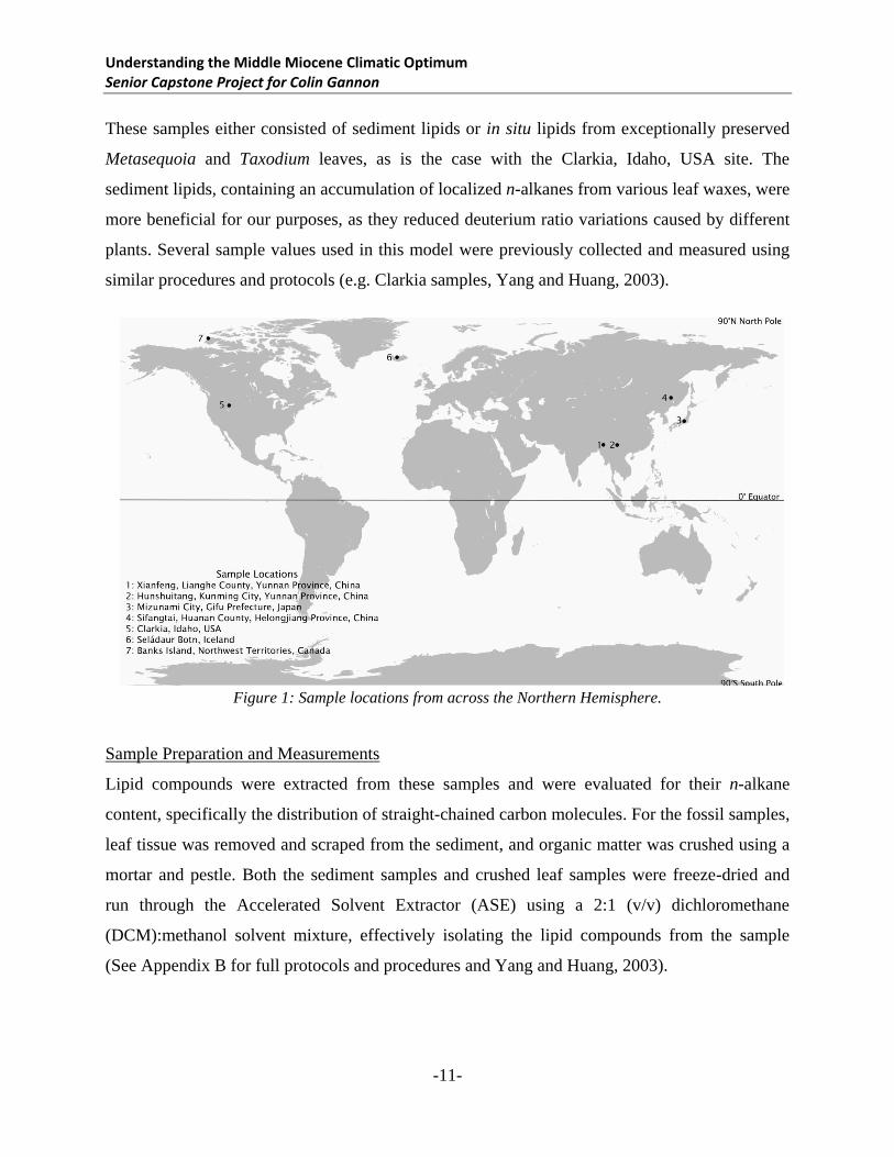
Our samples were collected from previously dated Middle Miocene deposits across the Northern
Hemisphere (Figure 1). In order to best capture a latitudinal trend and evaluate the equator-to-
pole temperature gradient, sample sites were selected at varying latitudes, ranging from 24° N to
74° N. Considering the small sample size (n=8), we targeted locations that were more or less
longitudinally unique to help achieve a mean distribution. No sample was collected from 98W
to 24E.
Understanding the Middle Miocene Climatic Optimum Senior Capstone Project for Colin Gannon
-11-
These samples either consisted of sediment lipids or in situ lipids from exceptionally preserved
Metasequoia and Taxodium leaves, as is the case with the Clarkia, Idaho, USA site. The
sediment lipids, containing an accumulation of localized n-alkanes from various leaf waxes, were
more beneficial for our purposes, as they reduced deuterium ratio variations caused by different
plants. Several sample values used in this model were previously collected and measured using
similar procedures and protocols (e.g. Clarkia samples, Yang and Huang, 2003).
Figure 1: Sample locations from across the Northern Hemisphere.
Sample Preparation and Measurements
Lipid compounds were extracted from these samples and were evaluated for their n-alkane
content, specifically the distribution of straight-chained carbon molecules. For the fossil samples,
leaf tissue was removed and scraped from the sediment, and organic matter was crushed using a
mortar and pestle. Both the sediment samples and crushed leaf samples were freeze-dried and
run through the Accelerated Solvent Extractor (ASE) using a 2:1 (v/v) dichloromethane
(DCM):methanol solvent mixture, effectively isolating the lipid compounds from the sample
(See Appendix B for full protocols and procedures and Yang and Huang, 2003).
Understanding the Middle Miocene Climatic Optimum Senior Capstone Project for Colin Gannon
-12-
Following the total lipid extraction, all samples underwent silica gel flash column
chromatography in which the first fraction, containing just the n-alkane molecules, was filtered
by solvents of increasing polarity. Samples were then run through a Flame Ionization Detector
(FID) on the GC to evaluate the quality and purity. Chromatographs with non-distinct peaks
were urea adducted, effectively stripping cyclic and branched alkanes from the targeted straight
n-alkanes. Samples were again processed by the FID. Evaluating the peak height produced on the
chromatograph, we determined the final concentration of sample for hydrogen isotope
measurement using Isotope-Ratio Mass-Spectrometer (IRMS) at Yale University (Yang et al.,
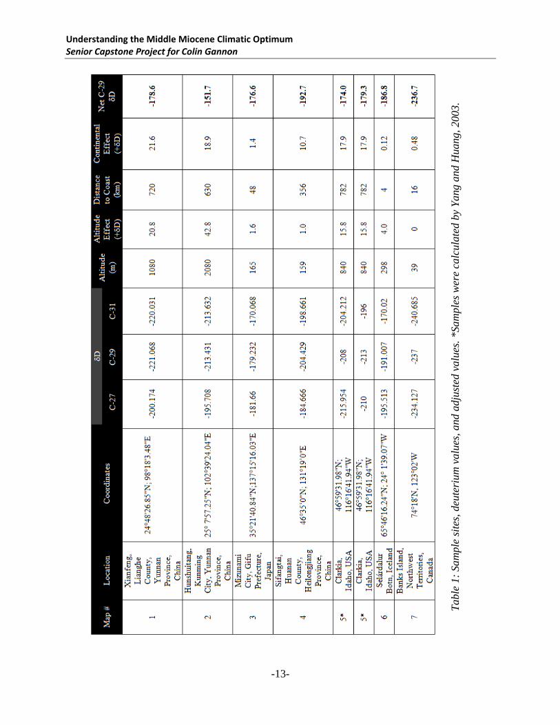
2011). The final value measured by the IRMS provided us with the ratio of deuterium to
hydrogen ( 2H/1H) on three (C-27, C-29, and C-31) n-alkane molecules (Table 1), expressed as
per mil (‰). These data, coupled with latitude, allow us to construct a model simulating the
meridional trend of deuterium.
Understanding the Middle Miocene Climatic Optimum Senior Capstone Project for Colin Gannon
-13-
Table
1:
Sam
ple
sit
es, deu
teri
um
valu
es, and a
dju
sted
valu
es.
*Sam
ple
s w
ere
calc
ula
ted b
y Y
ang a
nd H
uang, 2003
.
Understanding the Middle Miocene Climatic Optimum Senior Capstone Project for Colin Gannon
-14-
DATA ANALYSIS
The IRMS measurement produced a ratio of heavy hydrogen (deuterium) to hydrogen in the
range of -150 to -250‰. Although this standalone value did not explicitly provide much insight,
comparing relative magnitudes to other samples from the time period allowed us to establish a
trend with respect to latitude. Evaluations of this trend lead to construction of our model;
measuring a change in a single value, deuterium, across a linear (meridional) axis, while zonally
averaging the vertical component (i.e. altitude), we developed one-dimensional analysis. This
simulation provided us with an evaporation-precipitation relationship across a range of latitudes.
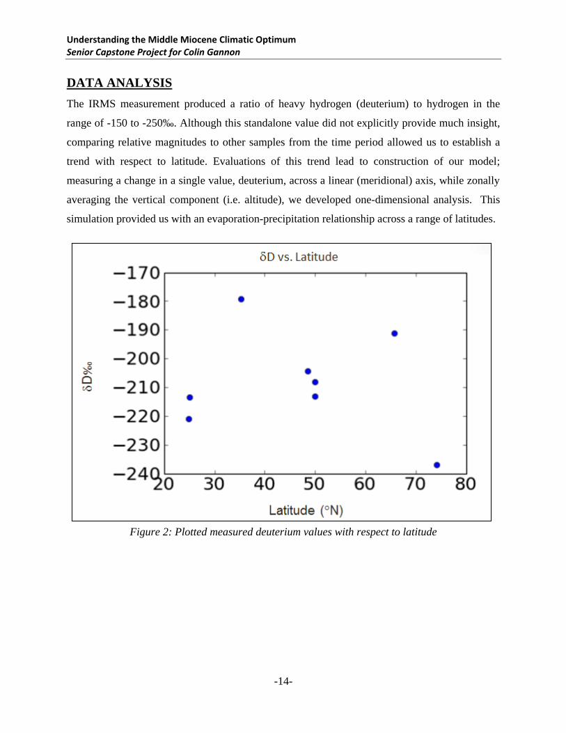
Figure 2: Plotted measured deuterium values with respect to latitude
Understanding the Middle Miocene Climatic Optimum Senior Capstone Project for Colin Gannon
-15-
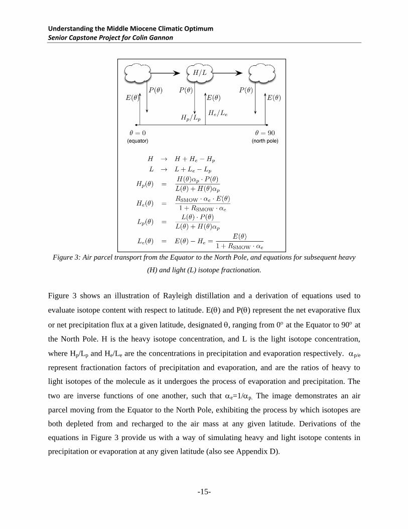
Figure 3: Air parcel transport from the Equator to the North Pole, and equations for subsequent heavy
(H) and light (L) isotope fractionation.
Figure 3 shows an illustration of Rayleigh distillation and a derivation of equations used to
evaluate isotope content with respect to latitude. E() and P() represent the net evaporative flux
or net precipitation flux at a given latitude, designated , ranging from 0 at the Equator to 90 at
the North Pole. H is the heavy isotope concentration, and L is the light isotope concentration,
where Hp/Lp and He/Le are the concentrations in precipitation and evaporation respectively. p/e
represent fractionation factors of precipitation and evaporation, and are the ratios of heavy to
light isotopes of the molecule as it undergoes the process of evaporation and precipitation. The
two are inverse functions of one another, such that e=1/p. The image demonstrates an air
parcel moving from the Equator to the North Pole, exhibiting the process by which isotopes are
both depleted from and recharged to the air mass at any given latitude. Derivations of the
equations in Figure 3 provide us with a way of simulating heavy and light isotope contents in
precipitation or evaporation at any given latitude (also see Appendix D).
Understanding the Middle Miocene Climatic Optimum Senior Capstone Project for Colin Gannon
-16-
Model Description
Our model, written in the Python programming language, is a one-dimensional evaluation of
evaporation and precipitation across a meridional axis related to D in precipitation. We
constructed two model simulations (each running for Miocene and Modern). The first interprets
evaporation minus precipitation (E-P) meridionally based on the data provided by our IRMS
measurements. The second model adjusted values to accommodate for additional fractionation
factors in both evaporation and precipitation. These factors, proposed by Dansgaard (1964) and
Jouzel (1997), allowed us to adjust the values of each specific sample to negate any geographic
variations and normalize towards fractionation driven entirely by atmospheric temperature and
latitude. The process is described in the “Adjusted Model Description” section.
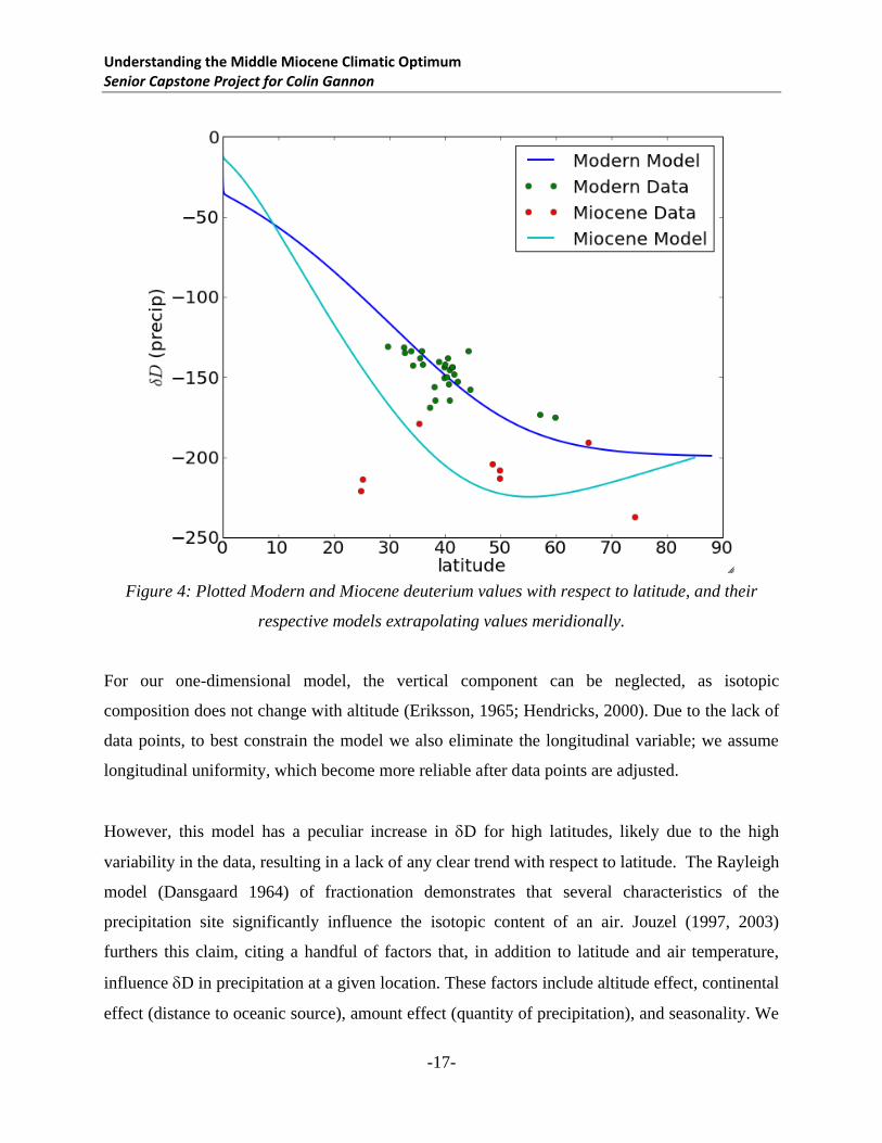
Figure 4 expresses the Middle Miocene trend plotting deuterium values and latitude, with the
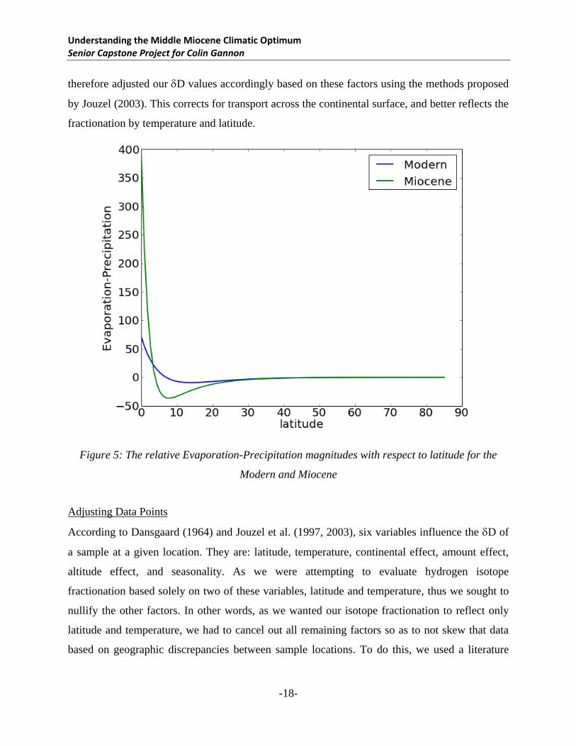
modern data included for comparison. Figure 5 is a simple model simulation of the E-P
relationship as latitude increases. It is important to note in both the modern simulation and
Miocene simulation, E-P ratio levels off at approximately 20N, fitting into the relatively
horizontal trend provided by the data points.
The challenge of simulating the precipitation and evaporation curves by this method is that we
have many unknown variables and only a handful of parameters. Therefore, we had to use
modern precipitation and evaporation to roughly "sketch out" the shape of the curves, and then
adjust those approximations to fit our Middle Miocene samples. It was also helpful to use
temperature approximations from the MMCO (You and Huber, 2003), to aid in the illustration of
temperature distributions across latitudes.
D measurements provided us with a scattered trend that didn't exhibit any significant trend
relative to latitude for Middle Miocene (see Figure 2). The D values did consistently register
more negative relative to current samples, collected from Metasequoia leaves (Yang et al., 2011)
(Figure 4). When the two data sets are curve fitted, the negative sloping trend of the Modern
samples is more plausible; the Miocene curve is more problematic, with more data points
varying from the mean trend.
Understanding the Middle Miocene Climatic Optimum Senior Capstone Project for Colin Gannon
-17-
Figure 4: Plotted Modern and Miocene deuterium values with respect to latitude, and their
respective models extrapolating values meridionally.
For our one-dimensional model, the vertical component can be neglected, as isotopic
composition does not change with altitude (Eriksson, 1965; Hendricks, 2000). Due to the lack of
data points, to best constrain the model we also eliminate the longitudinal variable; we assume
longitudinal uniformity, which become more reliable after data points are adjusted.
However, this model has a peculiar increase in D for high latitudes, likely due to the high
variability in the data, resulting in a lack of any clear trend with respect to latitude. The Rayleigh
model (Dansgaard 1964) of fractionation demonstrates that several characteristics of the
precipitation site significantly influence the isotopic content of an air. Jouzel (1997, 2003)
furthers this claim, citing a handful of factors that, in addition to latitude and air temperature,
influence D in precipitation at a given location. These factors include altitude effect, continental
effect (distance to oceanic source), amount effect (quantity of precipitation), and seasonality. We
Understanding the Middle Miocene Climatic Optimum Senior Capstone Project for Colin Gannon
-18-
therefore adjusted our D values accordingly based on these factors using the methods proposed
by Jouzel (2003). This corrects for transport across the continental surface, and better reflects the
fractionation by temperature and latitude.
Figure 5: The relative Evaporation-Precipitation magnitudes with respect to latitude for the
Modern and Miocene
Adjusting Data Points
According to Dansgaard (1964) and Jouzel et al. (1997, 2003), six variables influence the D of
a sample at a given location. They are: latitude, temperature, continental effect, amount effect,
altitude effect, and seasonality. As we were attempting to evaluate hydrogen isotope
fractionation based solely on two of these variables, latitude and temperature, thus we sought to
nullify the other factors. In other words, as we wanted our isotope fractionation to reflect only
latitude and temperature, we had to cancel out all remaining factors so as to not skew that data
based on geographic discrepancies between sample locations. To do this, we used a literature

Understanding the Middle Miocene Climatic Optimum Senior Capstone Project for Colin Gannon
-19-
survey to find the degree to which these variables influence the D values, and then adjusted our
collected data points accordingly.
Altitude effect
Poage and Chamberlain (2001) estimated the relationship of elevation to isotope fractionation.
Within a reasonable confidence interval, they are able to empirically link 18
O to elevation using
a linear regression. Similarly, using the Global Meteoric Water Line formula theorized by Craig
(1961), we can estimate the fluctuation of deuterium in precipitation based on altitude.
Two data points that would be significantly impacted by altitude are the Xianfeng and
Hunshuitang (#1 and #2 in Figure 1) which have modern elevations of 1080 meters and 2080
meters respectively. Currie (2005) and Rowley (2001) suggested that the Tibetan plateau reached
its current elevation by the end of the Middle Miocene after a significant uplift in the early
Miocene. Additionally, Chung et al. (1998) indicate that the southeaster edge of the Tibetan
Plateau and Yangtze Block (where these samples are located) was elevated by geologic
processes from the late Paleogene (40-30 Ma). It is ultimately fair to assume the altitude of these
locations is roughly similar to modern day. Smiley (1985) found that the Northern Idaho region
has stayed at a similar altitude since the Neogene, which includes the Miocene period. For all
other data points, modern elevation is also assumed (the magnitude of D is not that large as they
have relatively low altitudes).
Using the modern elevation of these samples in the regression in Poage and Chamberlain (2001),
we calculated the change in 18
O with respect to altitude.
where y is the change in 18
O and x is the altitude in meters. The resulting value is a negative
number that quantifies the underrepresentation caused by altitude. Since this estimates 18
O and
we are interested in D, we convert our C-29 D values to 18
O, using the linear Global Meteoric
Water Line (Craig, 1961).
Understanding the Middle Miocene Climatic Optimum Senior Capstone Project for Colin Gannon
-20-
8 ‰
After converting to 18
O, we subtracted the Poage and Chamberlain (2001) altitude adjusted
values (making the value less negative), and then converted back to D.
The Poage and Chamberlain (2001) formula is a parabolic estimation, and “zeros” or crosses the
x-axis at 111m above sea level, such that any sample site with an elevation below this altitude
would not be subject to altitude effect. Consequently, the Banks Island site (elevation of 40m)
was not adjusted for altitude effect.
Continental effect
Continental effect is one of the more complex factors to estimate, as it is largely dependent upon
the mechanisms for delivering precipitation to a given location, as well as seasonal patterns and
orography. However, some work has been done to generally approximate D value fluctuations
based on distance from the oceanic source. Rozanski (1981) found a gradient of -3.3‰/100km in
summer months and -1.3‰/100km in the winter months. Sonntag (1976, 1978) found a winter
season gradient of -2.4‰/100km and a similar summer season trend, while Salati et al. (1979)
found a -0.6‰/100km trend in the Amazon Basin. Considering these findings, we used a
conservative approximation favoring the Rozanski summer estimation, setting the gradient to -
3.0‰/100km.
The Middle Miocene saw high variance in sea levels, which were eventually stabilized following
the MMCO. The highest amplitude variations occurred from ~16-14 Ma, with a movement
towards a more permanent sea level fall at 14.2 Ma. This semi-permanence was likely result of
the East Antarctic Ice Sheet (EAIS) growth which brought increased stability to the oceans
(Flower et al. 1994). Using averages and trends from previous models, the maximum sea level
may be estimated at 100m higher than present, although for modeling purposes, a conservative
level is 50m in a time frame of ~15Ma (You 2009).
Understanding the Middle Miocene Climatic Optimum Senior Capstone Project for Colin Gannon
-21-
Thusly, for purposes of our model we assumed that sea level had little impact on continental
effect, and therefore used modern day values for distance from coast. We also knew, from the
locations of our data points, that sea level rise could not have been too dramatic during the
MMCO as several locations are located within close proximity to the coast (as little as 4 km in
the case of the Selárdalur Botn, Iceland sample). The samples that would be susceptible to
substantial continental effect would be the data points [1, 2, 3, 4, 5, and 7].
We then assigned the change in D values from continental effect, assuming current distance to
the coast. The Xiangfeng City (#1 in Figure 1) is approximately 700km from the South China
Sea, yielding a change of -21.6‰, Hunshuitang is 630km from its oceanic source, and thus is
overrepresented by 18.9‰, Mizunami (#3) is altered by 1.44‰, Sifangtai (#4) by 10.68‰,
Clarkia (#5) by 18‰, Selárdalur Botn (#6) has almost no quantifiable change (0.12‰), and
Banks Island (#7) 0.48‰.
Amount effect
Amount effect is exceedingly difficult to estimate without observational data, and can only be
assumed to be high in the tropics, leading to further uncertainty within this region. Therefore, we
ignored amount effect while tuning our data points, instead relying upon the E() and P()
parameters based upon modern data to model amount effect. Our lack of data at the tropics,
where amount effect has the most influence on isotope fractionation, makes neglecting this
variable less of a concern.
Seasonality effect
The seasonality effect may also be neglected for our purposes. Because the majority of our
samples were sediment samples, seasonality is more or less neutralized. This is because our D
values were obtained from a compilation of plant leaf waxes from all plants of the area and
deposited over a time transcending seasons. While it is true that these samples (particularly at the
highest latitudes) may disproportionately favor spring and summer seasons (that is, when the
plant is growing and absorbing groundwater), we had no clear way of defining the seasonal
impact and must therefore assume that each of our samples were proportionally effected by
seasonality.
Understanding the Middle Miocene Climatic Optimum Senior Capstone Project for Colin Gannon
-22-
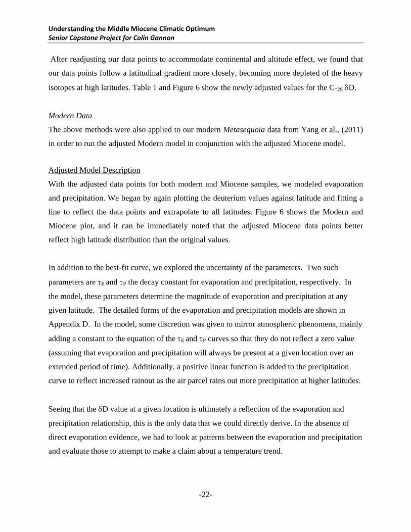
After readjusting our data points to accommodate continental and altitude effect, we found that
our data points follow a latitudinal gradient more closely, becoming more depleted of the heavy
isotopes at high latitudes. Table 1 and Figure 6 show the newly adjusted values for the C-29 D.
Modern Data
The above methods were also applied to our modern Metasequoia data from Yang et al., (2011)
in order to run the adjusted Modern model in conjunction with the adjusted Miocene model.
Adjusted Model Description
With the adjusted data points for both modern and Miocene samples, we modeled evaporation
and precipitation. We began by again plotting the deuterium values against latitude and fitting a
line to reflect the data points and extrapolate to all latitudes. Figure 6 shows the Modern and
Miocene plot, and it can be immediately noted that the adjusted Miocene data points better
reflect high latitude distribution than the original values.
In addition to the best-fit curve, we explored the uncertainty of the parameters. Two such
parameters are E and P the decay constant for evaporation and precipitation, respectively. In
the model, these parameters determine the magnitude of evaporation and precipitation at any
given latitude. The detailed forms of the evaporation and precipitation models are shown in
Appendix D. In the model, some discretion was given to mirror atmospheric phenomena, mainly
adding a constant to the equation of the E and P curves so that they do not reflect a zero value
(assuming that evaporation and precipitation will always be present at a given location over an
extended period of time). Additionally, a positive linear function is added to the precipitation
curve to reflect increased rainout as the air parcel rains out more precipitation at higher latitudes.
Seeing that the D value at a given location is ultimately a reflection of the evaporation and
precipitation relationship, this is the only data that we could directly derive. In the absence of
direct evaporation evidence, we had to look at patterns between the evaporation and precipitation
and evaluate those to attempt to make a claim about a temperature trend.
Understanding the Middle Miocene Climatic Optimum Senior Capstone Project for Colin Gannon
-23-
Figure 6: The original and adjusted data points and lines of best fit for the adjusted data. In the
top graph showing the Modern, data points are altered only slightly. The difference is more
substantial for the bottom graph depicting Miocene D values.
Understanding the Middle Miocene Climatic Optimum Senior Capstone Project for Colin Gannon
-24-
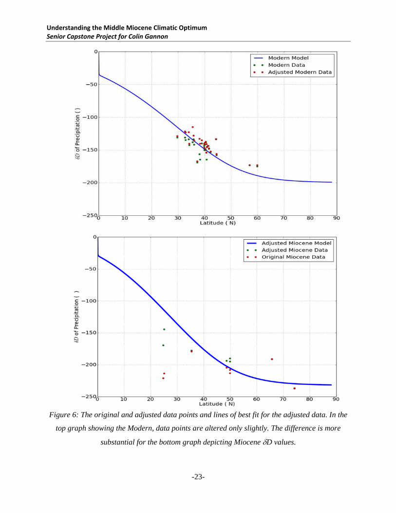
With only these variables, we compared the E and P parameters and established a relationship
between the two. Using a Bayesian Parameter estimation, we aimed to assess the significance of
E and P, and the correlations between the two. In other words, given the data, the model
estimates how the evaporation and precipitation curves are constrained. This is accomplished
with a Markov Chain Monte Carlo (MCMC), a simulation technique drawing random samples
from parameter probability distributions to estimate the values of E and P and their uncertainty,
based upon the data provided. With this, the best fits and magnitude of uncertainty for E and P
are established (see Figures 7 and 8).
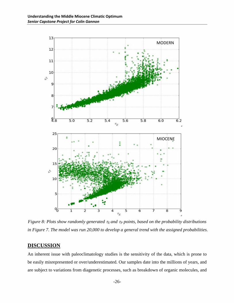
The E and P distributions provided by the MCMC could then be run concurrently, with E on
one axis and P on another. Run with many iterations (in this case, 20,000), a plot emerges based
on the probability drawings of each parameter. Parameters that have closer relationships (e.g.
both values increasing) indicate higher levels of certainty and prove correlation. A sporadic plot
would imply parameter estimates that have high uncertainty and are not correlated. For E and P,
the relationship must be well correlated, as evaporation and precipitation are generally inversely
related.
MODERN
Understanding the Middle Miocene Climatic Optimum Senior Capstone Project for Colin Gannon
-25-
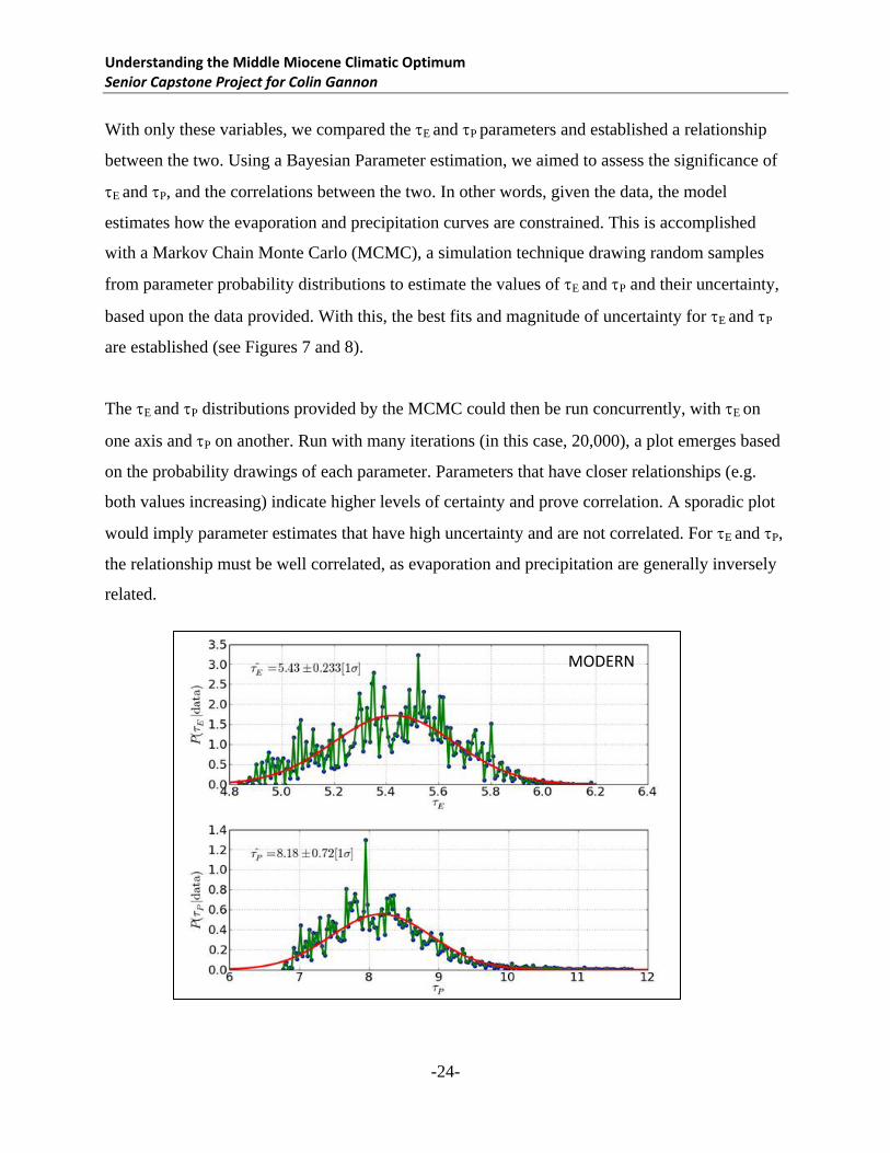
Figure 7: The probability distributions for E and P for the Modern and Miocene. The curves
produce a range for E and P values, based on the data provided.
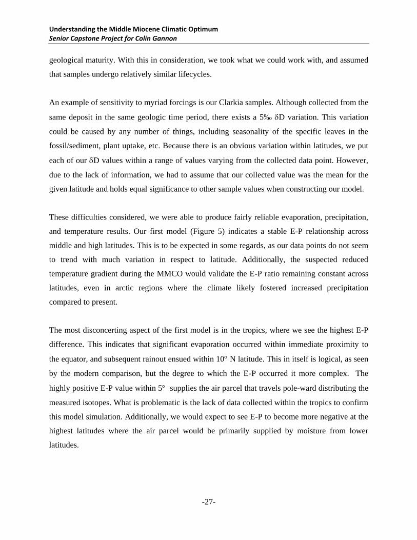
Figure 8 shows the MCMC evaluation of the Modern and Miocene simulations. It is clearly
evident from comparing the two that there is a more distinct trend during the Modern, which is
derived mainly from the presence of more data points, and consequently a higher confidence
margin. It is important to note, however, that the Miocene MCMC still derives a fairly distinct
trend in which the parameters are correlated. Despite more noise (a result of few data points), we
found an equation for the relationship between E and P which can be used to derive both
moisture and temperature distributions.
MIOCENE
Understanding the Middle Miocene Climatic Optimum Senior Capstone Project for Colin Gannon
-26-
Figure 8: Plots show randomly generated E and P points, based on the probability distributions
in Figure 7. The model was run 20,000 to develop a general trend with the assigned probabilities.
DISCUSSION
An inherent issue with paleoclimatology studies is the sensitivity of the data, which is prone to
be easily misrepresented or over/underestimated. Our samples date into the millions of years, and
are subject to variations from diagenetic processes, such as breakdown of organic molecules, and
MODERN
MIOCENE
Understanding the Middle Miocene Climatic Optimum Senior Capstone Project for Colin Gannon
-27-
geological maturity. With this in consideration, we took what we could work with, and assumed
that samples undergo relatively similar lifecycles.
An example of sensitivity to myriad forcings is our Clarkia samples. Although collected from the
same deposit in the same geologic time period, there exists a 5‰ D variation. This variation
could be caused by any number of things, including seasonality of the specific leaves in the
fossil/sediment, plant uptake, etc. Because there is an obvious variation within latitudes, we put
each of our D values within a range of values varying from the collected data point. However,
due to the lack of information, we had to assume that our collected value was the mean for the
given latitude and holds equal significance to other sample values when constructing our model.
These difficulties considered, we were able to produce fairly reliable evaporation, precipitation,
and temperature results. Our first model (Figure 5) indicates a stable E-P relationship across
middle and high latitudes. This is to be expected in some regards, as our data points do not seem
to trend with much variation in respect to latitude. Additionally, the suspected reduced
temperature gradient during the MMCO would validate the E-P ratio remaining constant across
latitudes, even in arctic regions where the climate likely fostered increased precipitation
compared to present.
The most disconcerting aspect of the first model is in the tropics, where we see the highest E-P
difference. This indicates that significant evaporation occurred within immediate proximity to
the equator, and subsequent rainout ensued within 10 N latitude. This in itself is logical, as seen
by the modern comparison, but the degree to which the E-P occurred it more complex. The
highly positive E-P value within 5 supplies the air parcel that travels pole-ward distributing the
measured isotopes. What is problematic is the lack of data collected within the tropics to confirm
this model simulation. Additionally, we would expect to see E-P to become more negative at the
highest latitudes where the air parcel would be primarily supplied by moisture from lower
latitudes.
Understanding the Middle Miocene Climatic Optimum Senior Capstone Project for Colin Gannon
-28-
Evaporation and precipitation relationships are classically difficult to evaluate at low latitudes.
The Intertropical Convergence Zone (ITCZ) influences seasonal rainout fluctuations and induces
strong horizontal advection patterns which are difficult to capture in our 1-D model. High rates
of evaporation year-round and subsequent high rates of precipitation do not allow for a strong
meridional trend to develop within the range of 0 to 10 N. The latitudinal temperature
gradient is small in these latitudes, and relatedly so is water content relative to latitude
(Hendricks, 2000). The stability of this region, regardless of climatic variations in mid and high
latitudes, makes linking gradient variations <10 difficult to extent to higher latitudes.
Furthermore, a lack of Middle Miocene proxy data further complicates simulation. Therefore, we
must use our data from the middle and high latitudes to project the positive E-P flux within the
tropical zone. Although this method does not necessarily yield accurate representation for these
latitudes, it does satisfy the development of our model, as we can approximate the flux and use it
as a parameter for net rainout in middle latitudes.
Some difficulty also arises in producing explicit, stand-alone results. We worked only with two
parameters, evaporation and precipitation, and therefore had no way of assessing the exact
magnitude of these values. That is, we could not produce a value dictating the specific amount of
evaporation we have a given location. We could, however, sum up the relative E and P curves
with respect to one another and to the Modern simulation. Without the assistance of other
parameters to refine our evaporation and precipitation, all subsequent results were relative.
When we ultimately ran the adjusted model, we began to develop a better picture of evaporation
and precipitation with respect to latitude, as well as improve our confidence intervals for
parameter correlation. Our simple plot (Figure 6) showed a much more promising and intuitive
D curve across latitudes than our first rendering (Figure 4). Seeing a trend that more closely
mimicked Modern data indicated a step in the right direction. The running of the MCMC chain
showed a high correlation between the E and P parameters (for both Modern and Miocene).
Even despite the small data set of eight, we were able to find well correlated parameters and a
reliable model.
Understanding the Middle Miocene Climatic Optimum Senior Capstone Project for Colin Gannon
-29-
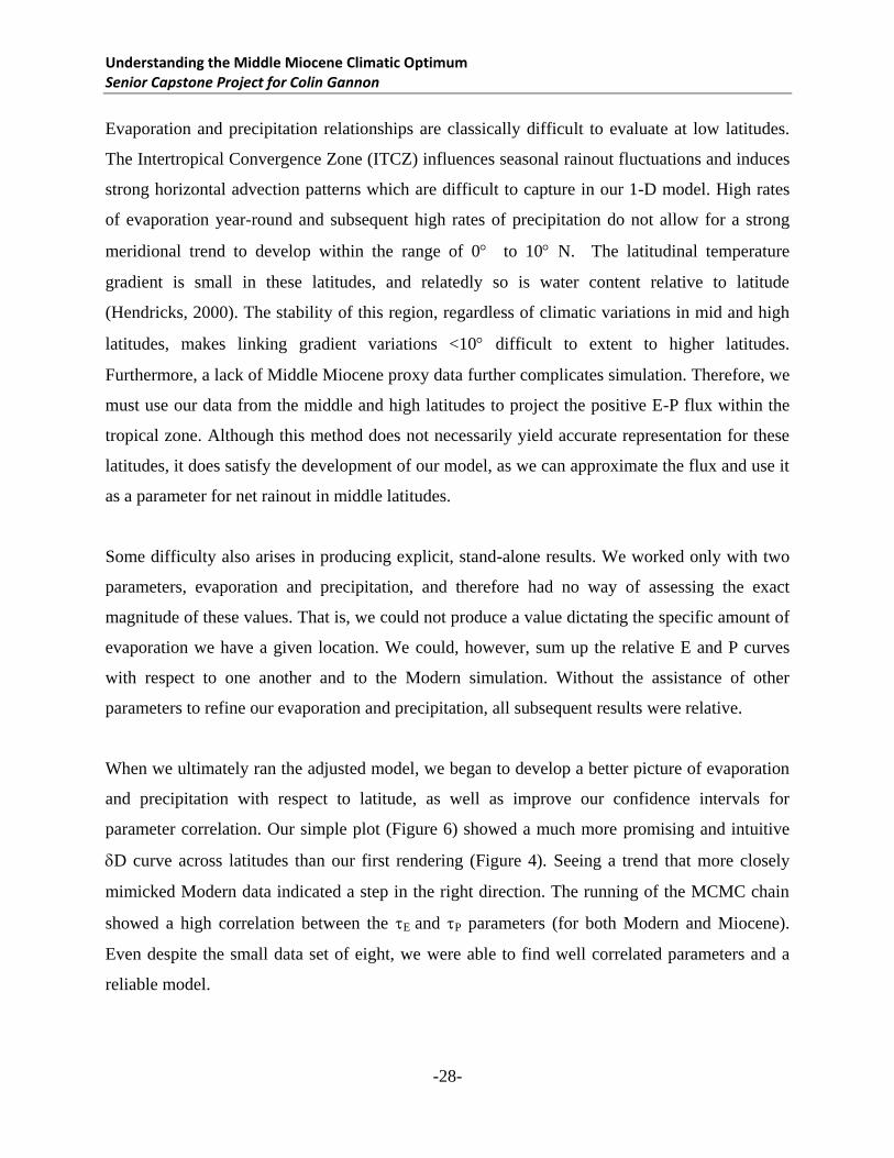
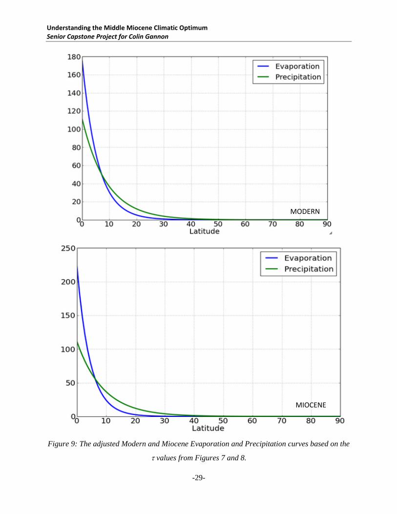
Figure 9: The adjusted Modern and Miocene Evaporation and Precipitation curves based on the
values from Figures 7 and 8.
MODERN
MIOCENE
Understanding the Middle Miocene Climatic Optimum Senior Capstone Project for Colin Gannon
-30-
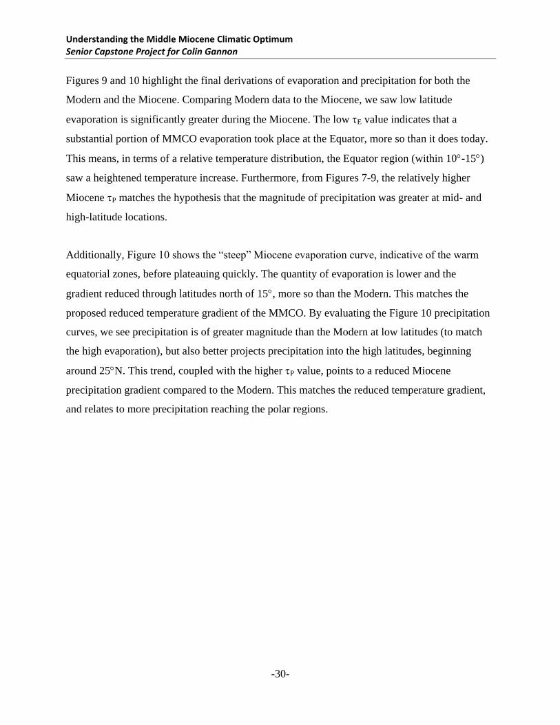
Figures 9 and 10 highlight the final derivations of evaporation and precipitation for both the
Modern and the Miocene. Comparing Modern data to the Miocene, we saw low latitude
evaporation is significantly greater during the Miocene. The low E value indicates that a
substantial portion of MMCO evaporation took place at the Equator, more so than it does today.
This means, in terms of a relative temperature distribution, the Equator region (within 10-15)
saw a heightened temperature increase. Furthermore, from Figures 7-9, the relatively higher
Miocene P matches the hypothesis that the magnitude of precipitation was greater at mid- and
high-latitude locations.
Additionally, Figure 10 shows the “steep” Miocene evaporation curve, indicative of the warm
equatorial zones, before plateauing quickly. The quantity of evaporation is lower and the
gradient reduced through latitudes north of 15, more so than the Modern. This matches the
proposed reduced temperature gradient of the MMCO. By evaluating the Figure 10 precipitation
curves, we see precipitation is of greater magnitude than the Modern at low latitudes (to match
the high evaporation), but also better projects precipitation into the high latitudes, beginning
around 25N. This trend, coupled with the higher P value, points to a reduced Miocene
precipitation gradient compared to the Modern. This matches the reduced temperature gradient,
and relates to more precipitation reaching the polar regions.
Understanding the Middle Miocene Climatic Optimum Senior Capstone Project for Colin Gannon
-31-
Figure 10: A comparison of the Modern and Miocene evaporation and precipitation curves, and
their respective magnitude relative to latitude.
CONCLUSIONS
Finding the E and P for both the Modern and the Miocene, we found the relative distributions of
evaporation and precipitation across a latitudinal axis. The Modern E approximation is larger
than the Miocene estimation, indicating that evaporation has a relatively higher magnitude at
lower latitudes during the Miocene. This implies that, compared to mid- to high-latitudes, more
evaporation occurs at the equator than during the Modern. We also saw a lower P during the
Miocene than during the Modern. This correlates to higher precipitation at higher latitudes, a
rainout pattern that could only exist with a small temperature gradient. That is, a sharper
temperature gradient at the upper latitudes, similar to today, would prevent much precipitation
from reaching the polar regions. With our significant and correlated E and P, we found that the
temperature distribution during the Miocene concentrated most of the heat at lower latitudes, and
then evenly distributed that trend up to the poles. Although we were unable to find explicit
Understanding the Middle Miocene Climatic Optimum Senior Capstone Project for Colin Gannon
-32-
temperature values, we were able to develop a fairly detailed picture of relative evaporation,
precipitation, and temperature distributions and gradients during the MMCO.
ACKNOWLEDGEMENTS
We would like to thank the NASA Rhode Island Space Grant for funding of this project, the
Bryant University Department of Science and Technology for use of their facilities and
equipment. I am grateful for Dr. Gerard Olack and Mr. Glendon Hunsinger of Yale University’s
Earth System Center for stable Isotopic Studies for technical support on hydrogen isotope
measurements, Dr. Xiaoyan Ruan of China University of Geoscience at Wuhan and a visiting
scholar at Bryant University for processing samples, Dr. Zekun Zhou (Kunming Botanical
Institute and Xishuangbanna Botanical Garden, Chinese Academy of Sciences), Dr. Chris
Williams (Franklin and Marshall College), and Dr. Fridgeir Grimsson (University Vienna)for
providing samples. Dr. Dan McNally served as a reviewer and read an early version of the
manuscript.
Understanding the Middle Miocene Climatic Optimum Senior Capstone Project for Colin Gannon
-33-
REFERENCES
Böhme, M., 2003. The Miocene Climatic Optimum: evidence from ectothermic vertebrates of
Central Europe. Palaeogeography, Palaeoclimatology, Paleoecology, 195: 389-401.
Bowen, G.J. and Revenaugh, J., 2003. Interpolating the isotopic composition of modern meteoric
precipitation. Water Resources Research, 39(10, 1299): SWC 9-1~13.
Chung, S.L., Lo, C.H., Lee, T.Y., Zhang, Y., Xie, Y., Li, X., Wang, K.L., Wang, P.L., 1998.
Diachronous uplift of the Tibetan plateau starting 40 Myr ago. Nature, 394: 769-773.
Craig, H., 1961. Isotopic variations in meteoric waters. Science, 133(3465): 1702-1703.
Currie, B.S., Rowley, D.B., Tabor, N.J., 2005. Middle Miocene paleoaltimetry of southern Tibet:
Implications for the role of mantle thickening and delamination in the Himalayan orogen.
Geology, 33(3): 181-184.
Dansgaard, W., 1964. Stable isotopes in precipitation. Tellus, 16(4): 436-468.
Eglinton, T., G. Eglinton, 2008. Molecular proxies for paleoclimatology. Earth and Planetary
Science Letters, 275: 1-16.
Eriksson, E., 1965. Deuterium and 18
O in precipitation and other natural waters; some theoretical
considerations. Tellus, 27: 498-512.
Farquhar, G.D., Cernusak, L.A., 2007. Heavy water fractionation during transpiration. Plant
Physiology, 143: 11-18.
Flower, B.P. and Kennett, J.P., 1994. The middle Miocene climatic transition: East Antarctic ice
sheet development, deep ocean circulation and global carbon cycling. Palaeogeography,
Palaeoclimatology, Paleoecology, 108: 537-555.
Gat, J.R., 1996. Oxygen and hydrogen isotopes in the hydrologic cycle Annu. Rev. Earth Planet.
Sci., 24: 225-262.
Henderson-Sellers, A., K. McGuffie, and Wiley, 1987. A Climate Modeling Primer.
Hendricks, M.B., D.J. DePaolo, R.C. Cohen, 2000. Space and time variation of δ18
O and δD in
precipitation: Can paleotemperature be estimated from ice cores? Global Biogeochemical
Cycles, 14(3): 851-861.
Holbourn, A., Kuhnt, W., Schulz, M. and Erlenkeuser, H., 2005. Impacts of orbital forcing and
atmospheric carbon dioxide on Miocene ice-sheet expansion. Nature, 438: 483-487.
Understanding the Middle Miocene Climatic Optimum Senior Capstone Project for Colin Gannon
-34-
Huang, Y., Shuman, B., Wang, Y., Webb T III, 2002. Hydrogen isotope ratios of palmitic acid in
lacustrine sediments record late-quaternary climate variations. Geology, 30: 1103-1106.
Jakobsson, M. et al., 2007. The early Miocene onset of a ventilated circulation regime in the
Arctic Ocean. Nature, 447: 986-990.
Joussame, S., Sadourny, R. and Jouzel, J., 1984. A general circulation model of water isotope
cycle in the atmosphere. Nature, 311: 24-29.
Jouzel, J., Alley, R.B., Cuffey, K.M., Dansgaard, W., Grootes, P., Hoffmann, G., Johnsen, S.J.,
Koster, R.D., Peel, D., Shuman, C.A., Stievenard, M., Stuiver, M., White, J., 1997.
Validity of the temperature reconstruction from water isotopes in ice cores. Journal of
Geophysical Research, 102(C12): 26,471-26,487.
Jouzel, J., Vimeux, F., Caillon, N., Delaygue, G., Hoffman, G., Masson-Delmotte, V., Parrenin,
F., 2003. Magnitutde of isotope/temperature scaling for interpretation of central Antarctic
ice cores. Journal of Geophysical Research: Atmospheres, 108(D12).
Kavanaugh, J.L., Cuffey, K.M., 2003. space and time variation of δ18
O and δD in Antarctic
precipitation revisited. Global Biogeochemical Cycles, 17(1): 1-14.
Kürschner, W.M., Kvaček, Z. and Dilcher, D.L., 2008. The impact of Miocene atmospheric
carbon dioxide fluctuations on climate and the evolution of terrestrial ecosystems.
Proceedings of the National Academy of Sciences, USA (PNAS), 105(2): 449-453.
Lee, J.E., Fung, I., DePaolo, D.J., Henning, C.C, 2007. Analysis of the global distribution of
water isotopes using the NCAR atmospheric general circulation model. Journal of
Geophysical Research: Atmospheres, 112(D16).
Leng, Q. and Yang, H., 2010. A new approach to reconstruct Paleogene atmospheric hydrology
at high latitudes. Science Foundation in China, 17(2): 46-49.
Leng, Q., Yang, H., Wang, L. and Li, C.-X., 2009. Discovery and evolution history of
Metasequoia. In: J.-G.e.-i.-c. Sha (Editor), Centennial Celebration of Chinese
Palaeontology. Science Press, Beijing, pp. 360-368 (in Chinese).
Liu, W.-G. and Yang, H., 2008. Multiple controls for the variability of hydrogen isotopic
compositions in higher plant n-alkanes from modern ecosystems. Global Change Biology,
14: 2166-2177.
Liu, W.-G., Yang, H. and Li, L.-W., 2006. Hydrogen isotopic compositions of n-alkanes from
terrestrial plants correlate with their ecological life forms. Oecologia, 150: 330-338.
Understanding the Middle Miocene Climatic Optimum Senior Capstone Project for Colin Gannon
-35-
Merlivat, L., Jouzel, J., 1979. Global Climatic Interpretation of the Deuterium-Oxygen 18
Relationship for Precipitation. Journal of Geophysical Research, 84(C8): 5029-5033.
Moberg, A., Sonechkin, D.M., Holmgren, K., Datsenko, N.M., Karlen, W., 2005. Highly
variable Northern Hemisphere temperatures reconstructed from low- and high-resolution
proxy data. Nature, 433(7026): 613-617
Micheels, A., Bruch, A.A., Uhl, D., Utescher, T. and Mosbrugger, V., 2007. A Late Miocene
climate model simulation with ECHAM4/ML and its quantitative validation with
terrestrial proxy data. Palaeogeography, Palaeoclimatology, Palaeoecology, 253: 251-270.
Müller, R.D., Sdrolias, M., Gaina, C., Steinberger, B., Heine, C., 2008. Long-Term Sea-Level
Flucturations Driven by Ocean Basin Dynamics. Science, 319(5868): 1357-1362.
Nathan, S.A. and Leckie, R.M., 2009. Early history of the Western Pacific Warm Pool during the
middle to late Miocene (~13.2-5.8 Ma): Role of sea-level change and implications for
equatorial circulation. Palaeogeography, Palaeoclimatology, Paleoecology, 274: 140-159.
Osborne, C.P., 2008. Atmosphere, ecology and evolution: what drove the Miocene expansion of
C4 grasslands? Journal of Ecology, 96(1): 35-45.
Poage, M.A., Page Chamberlain, C., 2001. Empirical Relationships Between Elevation and the
Stable Isotope Composition of Precipitation and Surface Waters: Considerations For
Studies of PaleoElevation Change. American Journal of Science, 301: 1-15.
Rogl, F., 1999. Mediterranean and Paratethys. Facts and Hypotheses of an Oligocene to Miocene
Paleogeography (short overview). Geologica Carpathica, 50: 339-349.
Royer, D.L. et al., 2001. Paleobotanical evidence for near present-day levels of atmospheric CO2
during part of the Tertiary. Science, 292(5525): 2310-2313.
Rozanski, K., Sonntag, C., Munnich, K.O., 1982. Factors controlling stable isotope compostion
of European precipitation. Tellus, 34: 142-150.
Shevenell, A.E., Kennett, J.P. and Lea, D.W., 2004. Middle Miocene Southern Ocean Cooling
and Antarctic Cryosphere Expansion. Science, 305: 1766-1770.
Sokolov, A.P. and Stone, P.H., 1998. A flexible climate model for use in integrated assessments.
Climate Dynamics, 14: 291-303.
Solomon, S. et al., 2007. Climate Change 2007: The Physical Science Basis. Contribution of
Working Group I to the Fourth Assessment Report of the Intergovernmental Panel on
Climate Change. Cambridge University Press, Cambridge, UK and NY, USA: .
Understanding the Middle Miocene Climatic Optimum Senior Capstone Project for Colin Gannon
-36-
Sonntag, C., Neureuther, P., Kalinke, C., Münnich, K., Klitzch, E., Weistroffer, K., 1976.
Paläoklimatik der Sahara- Ontinentaleffekt im Dund 18
O-Gehalt pluvialer Saharawässer.
Naturwissenschaften, 63: 497.
Sonntag, C., Klitzsch, E., Shazly, E.M., Kalinke, C., and Münnich, K.O., 1978. Paläoklimatische
Information im Isotopen-gehalt 14
C-datierter Saharawässer: Kontinentaleffekt in D und
18O. Geol. rundsch, 67: 413-423.
Speelman, E.N., Sewall, J.O., Noone, D., Huber, M., von der Heydt, A., Sinnighe Damste, J.,
Reichart, G. , 2010. Modeling the influence of a reduced equator-to-pole sea surface
temperature gradient on the distribution of water isotopes in the Early/Middle Eocene.
Earth and Planetary Science Letters, 298: 57-65.
Sturm, C., Zhang, Q. and Noone, D., 2010. An introduction to stable water isotopes in climate
models: benefits of forward proxy modeling for paleoclimatology. Clim. Past, 6: 115-129.
Verducci, M. et al., 2009. The Middle Miocene climatic transition in the Southern Ocean:
Evidence of paleoclimatic and hydrographic changes at Kerguelen plateau from
planktonic foraminifers and stable isotopes Palaeogeography, Palaeoclimatology,
Paleoecology, 280: 371-386.
Wang, C., Zhao, X., Liu, Z., Lippert, P.C., Graham, S.A., Coe, R.S., Yi, H., Zhu, L., Liu, S., Li,
Y., 2008. Constraints on the early uplift history of the Tibetan Plateau. PNAS, 105(13):
4987-4992.
White, J.W., 2004. Paleoclimate. Do I hear a million? Science, 304(5677): 1609-1610.
Witkowski, C., Gupta, N.S., Yang, H., Leng, Q., Williams, C.J., Briggs, D.E.G., and Summons,
R.E., 2012. Molecular preservation of Cenozoic conifer fossil lagerstatten from Banks
Island, the Canadian arctic. Palaios, 27: 279-287.
Yang, H., Blais, B. and Leng, Q., 2011. Stable isotope variations from cultivated Metasequoia
trees in the United States: A statistical approach to assess isotope signatures as climate
signals. Japanese Journal of Historical Botany (Special Issue of the proceedings of the
Third International Metasequoia Symposium, August 3-8, 2010, Osaka, Japan), 19(1-2):
75-88.
Yang, H. and Huang, Y.-S., 2003. Preservation of lipid hydrogen isotope ratios in Miocene
lacustrine sediments and plant fossils at Clarkia, northern Idaho, USA. Organic
Geochemistry, 34: 413-423.
Understanding the Middle Miocene Climatic Optimum Senior Capstone Project for Colin Gannon
-37-
Yang, H. and Leng, Q., 2009. Molecular hydrogen isotope analysis of living and fossil plants -
Metasequoia as an example. Progress in Natural Science, 19: 901-912.
Yang, H., Liu, W.-G., Leng, Q. and Hren, M.T.P., Mark, 2011. Variation in n-alkane δD values
from terrestrial plants at high latitude: Implications for paleoclimate reconstruction.
Organic Geochemistry, 42: 283-288.
Yao, M.S., Stone, P.H., 1987. Development of a Two-Dimensional Zonally Average Statistical-
Dynamical Model. Part 1: The Parameterization of Moist Convection and its Role in the
General Circulation. Journal of the Atmospheric Sciences, 44(1): 65-82.
You, Y., Huber, M., Muller, R.D., Poulsen, C.J. and Ribbe, J., 2009. Simulation of the Middle
Miocene Climate Optimum. Geophysical Research Letters, 36: 1-5.
Zachos, J., Pagani, M., Sloan., Thomas, E., Billups, K., 2001. Trends, Rhythms, and Aberrations
in Global Climate 65 Ma to Present. Science, 292: 686-693.
Understanding the Middle Miocene Climatic Optimum Senior Capstone Project for Colin Gannon
-38-
AFTERWORD
In our eyes, this multi-stage, interdisciplinary project successfully took a limited number of
Middle Miocene data points and created a working model simulating evaporation and
precipitation. Starting with fossil and sediment samples that served as proxies for climate during
the 15-17 million years, we were able to construct a latitudinal distribution of D values related
to precipitation. Although deposits containing MMCO climatic information is sparse, we
ultimately produced eight samples that sufficiently served our purposes.
We next purified the fossils and sediments and isolated the exact compounds related to hydrogen
isotope fractionation. At the end of the laboratory phase of the project, we had explicit D values
related to given latitudes. From these D values, we were able to derive the relationship between
evaporation and precipitation ranging from the Equator to the North Pole, and ultimately tie that
back into the temperature distribution of the time period.
The modeling phase was met with some setbacks, but in the end these issues were resolved by
adjusting our Miocene data points so that the D values only reflected latitude and air
temperature. With this tuning made, we saw an intuitive D with respect to latitude, and were
able to proceed with our model.
Through a process of parameter estimation, we arrived at our final results for distribution of
evaporation and precipitation, and relatedly, temperature. Most simply, our results showed that
during the Middle Miocene Climatic Optimum, the Earth was substantially warmer than Modern;
although, most of that heat was centered in the equatorial regions. Evaporation and precipitation
were also very high in these areas. However, as latitude increases and moves towards the poles,
evaporation drops off sharply, and precipitation is well distributed into the poles. In other words,
from the middle latitudes up to the North Pole, the precipitation and temperature distributions are
fairly balanced, more so than today.
This information presents value to the scientific community as a way of understanding the
processes related to atmospheric moisture transport and the relationships of evaporation and
temperature in a climate different than today. During the Middle Miocene, with a climate warmer
Understanding the Middle Miocene Climatic Optimum Senior Capstone Project for Colin Gannon
-39-
than Modern, the variations in magnitude and distribution of evaporation, precipitation, and
temperature may be an example of a future climate that we may soon be facing. It is important to
understand the relationship of these variables to garner better insight towards how the climate
behaves under certain conditions; consequently, we are satisfied with our contribution to this
discussion, and believe that the results we concluded can contribute to a greater cause of
understanding the Earth’s climate.

Understanding the Middle Miocene Climatic Optimum Senior Capstone Project for Colin Gannon
-40-
APPENDICES
Understanding the Middle Miocene Climatic Optimum Senior Capstone Project for Colin Gannon
-41-
Appendix A: Glossary
Term Explanation
D Read "delta D," this correlates to an empirical data point representing the
difference ratio of deuterium to hydrogen in a sample. It follows the
equation: D= 1000[(RSAMPLE - RVSMOW)/ RVSMOW]
Advection A process by which meteoric water is moved through the atmosphere.
Advection is the bulk transport of a substance through a medium. In this
case, advection is the process by which an air parcel is moved through the
atmosphere, transporting with it hydrogen isotopes.
Air mass See "Air parcel"
Air parcel A theoretical mass of atmospheric moisture that is transported by advective
and diffusive forces (i.e. by temperature and pressure differences). In this
context, it is assumed that an air parcel moves from the equator towards the
poles, driven primarily by advective processes. It is also from the air parcel
that precipitation containing a unique isotope signature is rained out.
Altitude effect A factor of isotope fractionation in precipitation in which locations at higher
altitude will be more depleted of heavy isotopes.
Amount effect A factor of isotope fractionation in precipitation in which locations with high
amounts of precipitation will have relatively higher abundances of heavy
isotopes.
Atmosphere One of the four interconnected "spheres" of the Earth. Relating to the gases
(including water vapor) within the gravitational range of the Earth.
Biosphere One of the four interconnected "spheres" of the Earth. Relating to all living
things and ecosystems.
Carbon dioxide A greenhouse gas emitted from the combustion of fossil fuels. It is suggested
its emission is responsible for modern day global warming. See also:
"Greenhouse gas."
Climate The sum of the parts of: precipitation, temperature, humidity, wind and
atmospheric pressure at a given location over an extended period of time.
Understanding the Middle Miocene Climatic Optimum Senior Capstone Project for Colin Gannon
-42-
Continental
effect
A factor of isotope fractionation in precipitation in which locations further
from the ocean will be more depleted in heavy isotopes
Deuterium They heavy isotope of hydrogen, containing 2 isotopes. May also be referred
to simply as "D" or "2H" in context. Deuterium is often present in the
atmosphere and biosphere in the form of heavy water, or HDO (as opposed
to H2O).
Diffusion A process by which meteoric water is moved through the atmosphere.
Diffusion is the transport of a substance through a medium without bulk
motion. In this case, diffusion is the process by which hydrogen isotopes are
transported through the atmosphere, although not necessarily within a bulk
air mass. In other words, diffusion would evenly distribute deuterium
molecules throughout the atmosphere in the absence of air parcel transport.
East Antarctic
Ice Sheet
Abbreviated EAIS, it is a section of Antarctica on the ocean. The expansion
and retraction of this ice sheet is has served as an indicator of global climate.
Eddies A circulation pattern that serves as a "ball-bearing" of sorts, moving in the
opposite direction of the drivers next to it. For example, a Ferrell cell, located
in-between Hadley and Polar cells, circulates air in the opposite direction as
its neighbors.
Epoch A length of time on the geologic scale, shorter than a period but longer than
an age.
Ferrell cell An atmospheric circulation pattern that sits in between, and is largely
dependent upon, the Hadley and Polar cells, as it exists as an eddy.
Fossil fuels Fuels from ancient biological matter created from chemical processes over
millions of years. The burning of these substances (including coal and oil)
generate electricity but also emits greenhouse gases into the atmosphere.
Fractionation The process by which a mixture is divided into fractions. Isotopic
fractionation is the process by which isotopes are separated from their
original solution. In the context of this research, isotopic fractionation is the
separation of water molecules containing deuterium from those containing
hydrogen in the atmosphere.
Understanding the Middle Miocene Climatic Optimum Senior Capstone Project for Colin Gannon
-43-
Geosphere One of the four interconnected "spheres" of the Earth. Relating to the rocks,
soil, and geologic portions of the Earth.
Global
Circulation
Model
Also referred to as a GCM, this is a computer generated model that analyzes
data points from across the globe to create a 3-dimensional reconstruction of
the Earth's climate. Although often criticized for their flaws, often in the
form of over/under signifying variables or physical equations, GCMs are the
most useful tool for simulating future climate scenarios.
Global Meteoric
Water Line
The average relationship between hydrogen and oxygen isotopes in water
worldwide. The generally accepted equation is: D = 8.0*18
O + 10‰ .
Greenhouse gas
(effect)
A gas that is released into the atmosphere and subsequently prevents radiated
heat from escaping the Earth. Higher levels of greenhouse gases in the
atmosphere relate to more heat being trapped, causing the temperature of the
Earth to rise.
Hadley cell An atmospheric circulation pattern that moves rising air from the Equator
and transports it poleward at a higher elevation, until returning the air to the
surface and area of high pressure, usually in the mid-latitudes.
Hydrologic cycle How water moves through the different spheres of the Earth. Most simply,
the process of evaporation from the surface, transport through the
atmosphere, precipitation, transport through the geosphere, hydrosphere, and
biosphere, ultimately returning to the atmosphere through evaporation on a
perpetual cycle.
Hydrosphere One of the four interconnected "spheres" of the Earth. Relating to the
movement of water throughout the atmosphere, geosphere, and biosphere.
in situ Latin for in position, this refers to a specimen or sample that has not been
moved or altered from its initial position.
Isotope An alteration in the number of neutrons in an element. For example, a
hydrogen atom most commonly contains 1 proton, 1 neutron, and 1 electron.
An isotope of hydrogen is deuterium, or heavy hydrogen, which has 1
proton, 2 neutrons, and 1 electron.
Isotope gradient The amount by which the isotope ratio changes over a given frame of
Understanding the Middle Miocene Climatic Optimum Senior Capstone Project for Colin Gannon
-44-
reference; in this case, the difference between isotope ratios at varying
latitudes.
Isotope ratio The ratio between a specific isotope and its most abundant form. In this case,
the ratio between deuterium and hydrogen (the most abundant form).
Isotopic
fractionation
See "Fractionation"
Isotopic
signature
The isotope ratio at a given point, relating to its intrinsic characteristics. In
this case, the ratio pertaining to evaporation and precipitation at a given
location.
Latitude A geographic coordinate, being a theoretical band on the Earth's surface that
denotes relative North or South location and runs east-west, parallel to the
Equator. 0° signifies the Equator, with 90°N and 90°S marking the
geographic North and South Poles respectively.
Latitudinal
gradient
The change in latitude between two points.
Lipid A classification type for molecules. Naturally occurring, lipids include fats,
sterols and waxes, among others. Lipids are found on the surface of leaves
and intrinsically hold the isotopic signature of water from root uptake.
Additionally, lipids are preserved extremely well over long time frames,
making it a valuable proxy when evaluating climates millions of years old.
Longitude A geographic coordinate, being a theoretical band on the Earth's surface
denoting relative East or West location running north to south, parallel to the
Prime Meridian. 0° signifies the Prime Meridian, ranging to 180° eastward
and westward
Meridionally Along a meridian; travelling across latitudes
Metasequoia A deciduous redwood tree. An ancient tree, this species has great value for
paleoclimatology, as the isotopic content of lipids preserved in its leaves
correlate well to deuterium in the atmosphere.
Meteoric water
content
The isotope and moisture content of water in the atmosphere at a given time
and location.
Understanding the Middle Miocene Climatic Optimum Senior Capstone Project for Colin Gannon
-45-
Middle Miocene A geologic timeframe occurring from 16-11.6 million years ago. It is a sub-
epoch of the Miocene, both of which occurred during the Neogene. See also
Appendix C.
Milankovitch
cycles
Changes in the Earth’s movements that influences global climate. The cycles
include eccentricity (the shape of the Earth’s orbit around the sun), obliquity
(the tilt of the Earth relative to its orbital plane), and axial precision (rotation
of Earth’s axis). All three have marked cycles on the magnitude of several
ten-thousand year periods, and are believed to play a large role in the
cyclical ice age patterns.
n-alkane A straight-chained molecule containing carbon and hydrogen atoms.
Orography
/orographic
features
Relating to mountain building processes and crustal uplift
Paleoclimate An ancient climate.
Polar cell An atmospheric circulation pattern that upwells air at mid-latitude (modern
day is approximately 60°N/S) and moves it through the atmosphere,
eventually returning it to the surface at the pole.
Protium The most naturally occurring isotope of hydrogen. May also be referred to
simply as hydrogen, or hydrogen's "light" isotope.
Proxy A piece of data that quantitatively relates to a piece of information about an
ancient climate
Rainout Precipitation heavy isotopes from the atmosphere at a given time and
location
Relative
humidity
The ratio between the partial pressure of water vapor and its saturated vapor
pressure. Dependent upon temperature and air pressure, relative humidity is
an important factor in the rates of evaporation and precipitation.
Seasonality A factor of isotope fractionation in precipitation in which different seasons
yield varying levels of heavy isotopes. It can be expected that during winter
months, precipitation will be more depleted of heavy isotopes relative to
summer months.

Understanding the Middle Miocene Climatic Optimum Senior Capstone Project for Colin Gannon
-46-
SMOW See "Vienna Standard Mean Ocean Water"
Solar insolation The amount of radiation from the sun at a given location over a certain
period of time. Solar insolation is prone to fluctuations from the sun’s energy
output, and has an effect on the Earth’s climate.
Temperature
gradient
The rate at which temperature changes between two points. In the context of
an Equator-to-Pole temperature gradient, it is the slope between the
temperature at the equator and the North/South pole.
Vienna Standard
Mean Ocean
Water
The accepted mean 2H/
1H ratio in ocean waters. The current standard, as
evaluated by the International Atomic Energy Agency is 155.76 ± 0.1 ppm.
VSMOW See "Vienna Standard Mean Ocean Water"
Well-preserved A sample that has not been subject to decay or weathering, making it a
candidate for use as a paleoclimate proxy.
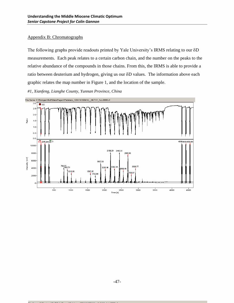
Understanding the Middle Miocene Climatic Optimum Senior Capstone Project for Colin Gannon
-47-
Appendix B: Chromatographs
The following graphs provide readouts printed by Yale University’s IRMS relating to our D
measurements. Each peak relates to a certain carbon chain, and the number on the peaks to the
relative abundance of the compounds in those chains. From this, the IRMS is able to provide a
ratio between deuterium and hydrogen, giving us our D values. The information above each
graphic relates the map number in Figure 1, and the location of the sample.
#1, Xianfeng, Lianghe County, Yunnan Province, China
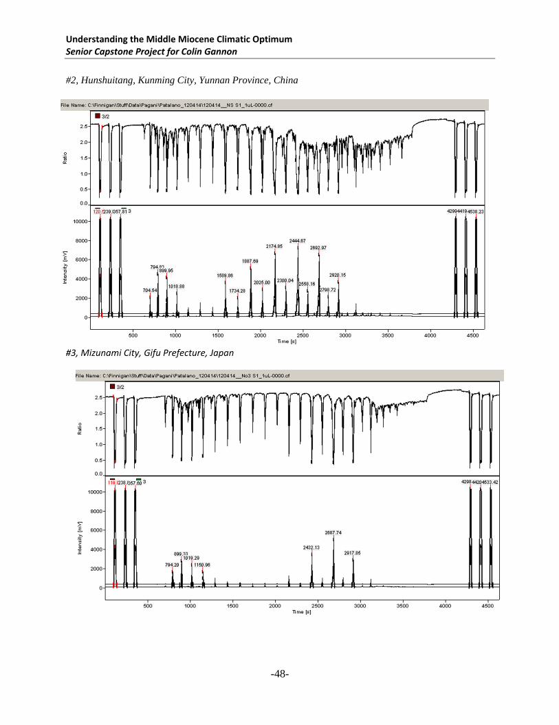
Understanding the Middle Miocene Climatic Optimum Senior Capstone Project for Colin Gannon
-48-
#2, Hunshuitang, Kunming City, Yunnan Province, China
#3, Mizunami City, Gifu Prefecture, Japan
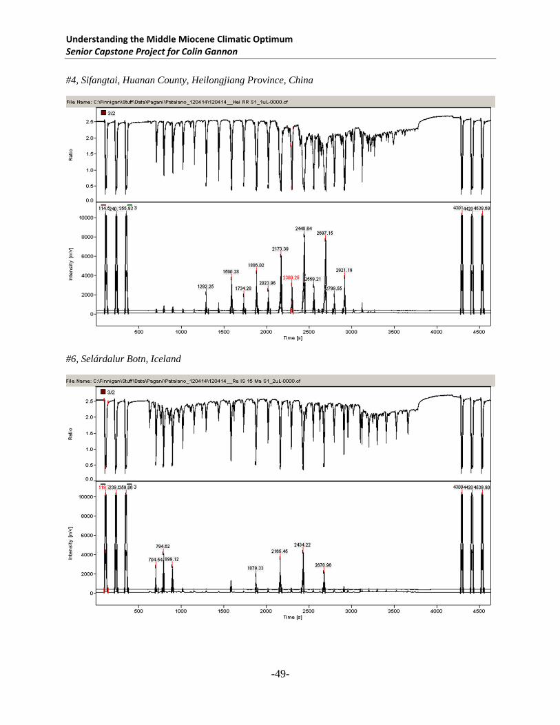
Understanding the Middle Miocene Climatic Optimum Senior Capstone Project for Colin Gannon
-49-
#4, Sifangtai, Huanan County, Heilongjiang Province, China
#6, Selárdalur Botn, Iceland
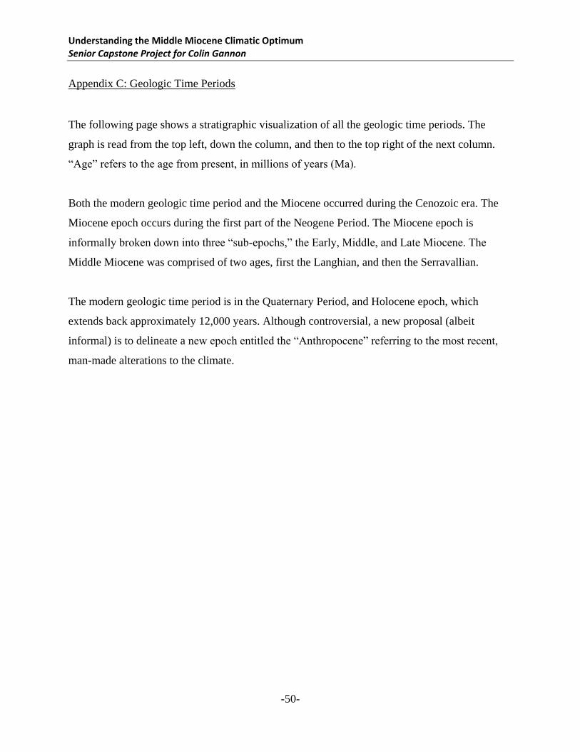
Understanding the Middle Miocene Climatic Optimum Senior Capstone Project for Colin Gannon
-50-
Appendix C: Geologic Time Periods
The following page shows a stratigraphic visualization of all the geologic time periods. The
graph is read from the top left, down the column, and then to the top right of the next column.
“Age” refers to the age from present, in millions of years (Ma).
Both the modern geologic time period and the Miocene occurred during the Cenozoic era. The
Miocene epoch occurs during the first part of the Neogene Period. The Miocene epoch is
informally broken down into three “sub-epochs,” the Early, Middle, and Late Miocene. The
Middle Miocene was comprised of two ages, first the Langhian, and then the Serravallian.
The modern geologic time period is in the Quaternary Period, and Holocene epoch, which
extends back approximately 12,000 years. Although controversial, a new proposal (albeit
informal) is to delineate a new epoch entitled the “Anthropocene” referring to the most recent,
man-made alterations to the climate.
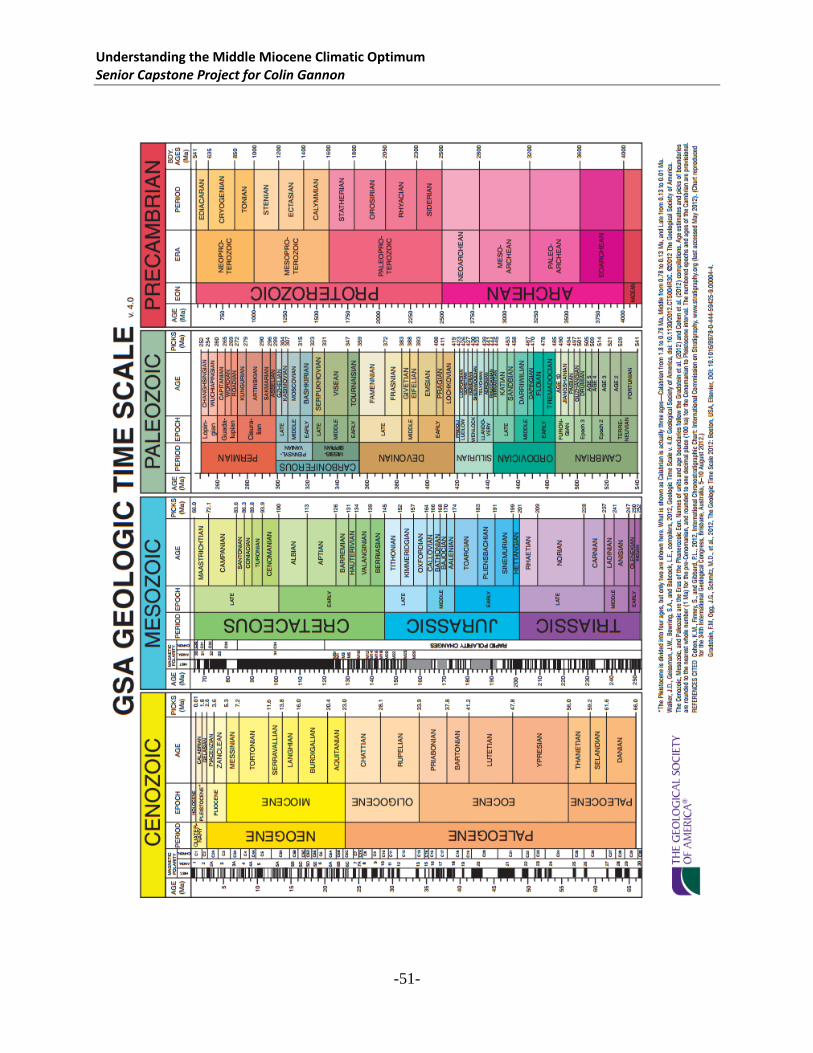
Understanding the Middle Miocene Climatic Optimum Senior Capstone Project for Colin Gannon
-51-
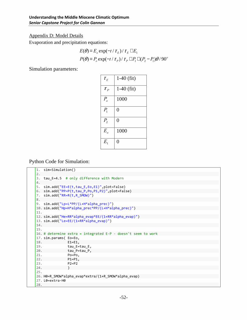
Understanding the Middle Miocene Climatic Optimum Senior Capstone Project for Colin Gannon
-52-
Appendix D: Model Details
Evaporation and precipitation equations:
E(q ) = Eo exp(-t /t E ) /t E +E1
P(q ) = Po exp(-t /t P ) /t P +P1 + (P2 -P1)q / 90o
Simulation parameters:
t E 1-40 (fit)
t P 1-40 (fit)
Po 1000
P1 0
P2 0
Eo 1000
E1 0
Python Code for Simulation:
1. sim=Simulation() 2. 3. tau_E=4.5 # only difference with Modern 4. 5. sim.add("EE=E(t,tau_E,Eo,E1)",plot=False) 6. sim.add("PP=P(t,tau_P,Po,P1,P2)",plot=False) 7. sim.add("RR=R(t,R_SMOW)") 8. 9. sim.add("Lp=L*PP/(L+H*alpha_prec)") 10. sim.add("Hp=H*alpha_prec*PP/(L+H*alpha_prec)") 11. 12. sim.add("He=RR*alpha_evap*EE/(1+RR*alpha_evap)") 13. sim.add("Le=EE/(1+RR*alpha_evap)") 14. 15. 16. # determine extra = integrated E-P - doesn't seem to work 17. sim.params( Eo=Eo, 18. E1=E1, 19. tau_E=tau_E, 20. tau_P=tau_P, 21. Po=Po, 22. P1=P1, 23. P2=P2 24. ) 25. 26. H0=R_SMOW*alpha_evap*extra/(1+R_SMOW*alpha_evap) 27. L0=extra-H0 28.
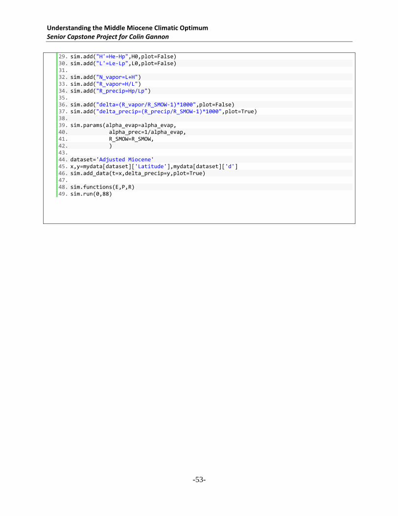
Understanding the Middle Miocene Climatic Optimum Senior Capstone Project for Colin Gannon
-53-
29. sim.add("H'=He-Hp",H0,plot=False) 30. sim.add("L'=Le-Lp",L0,plot=False) 31. 32. sim.add("N_vapor=L+H") 33. sim.add("R_vapor=H/L") 34. sim.add("R_precip=Hp/Lp") 35. 36. sim.add("delta=(R_vapor/R_SMOW-1)*1000",plot=False) 37. sim.add("delta_precip=(R_precip/R_SMOW-1)*1000",plot=True) 38. 39. sim.params(alpha_evap=alpha_evap, 40. alpha_prec=1/alpha_evap, 41. R_SMOW=R_SMOW, 42. ) 43. 44. dataset='Adjusted Miocene' 45. x,y=mydata[dataset]['Latitude'],mydata[dataset]['d'] 46. sim.add_data(t=x,delta_precip=y,plot=True) 47. 48. sim.functions(E,P,R) 49. sim.run(0,88)