The phase transition in

bounded-size Achlioptas processes

Lutz Warnke

University of Cambridge

Joint work with Oliver Riordan

Classical model

Paul Erdos

Alfred Renyi

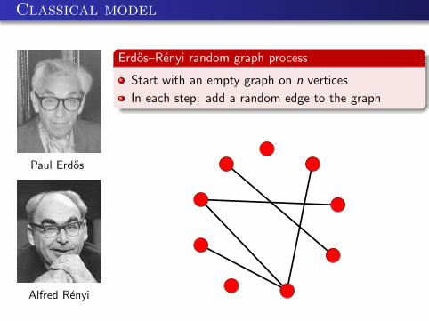
Erdos–Renyi random graph process

Start with an empty graph on n vertices

In each step: add a random edge to the graph

Classical model

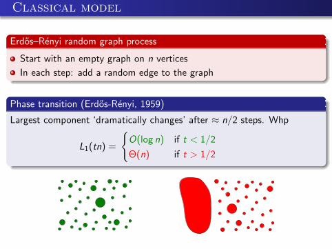
Erdos–Renyi random graph process

Start with an empty graph on n vertices

In each step: add a random edge to the graph

Phase transition (Erdos-Renyi, 1959)

Largest component ‘dramatically changes’ after ≈ n/2 steps. Whp

L1(tn) =

{

O(log n) if t < 1/2

Θ(n) if t > 1/2

Classical model

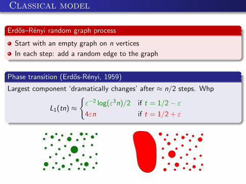
Erdos–Renyi random graph process

Start with an empty graph on n vertices

In each step: add a random edge to the graph

Phase transition (Erdos-Renyi, 1959)

Largest component ‘dramatically changes’ after ≈ n/2 steps. Whp

L1(tn) ≈

{

ε−2 log(ε3n)/2 if t = 1/2− ε

4εn if t = 1/2 + ε

Model with dependencies

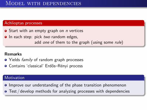
Achlioptas processes

Start with an empty graph on n vertices

In each step: pick two random edges,add one of them to the graph (using some rule)

Remarks

Yields family of random graph processes

Contains ‘classical’ Erdos–Renyi process

Motivation

Improve our understanding of the phase transition phenomenon

Test/develop methods for analyzing processes with dependencies

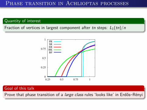
Phase transition in Achlioptas processes

Quantity of interest

Fraction of vertices in largest component after tn steps: L1(tn)/n

0

0.25

0.5

0.75

1

0.25 0.5 0.75 1

PR

SR

ER

BK

BF

Goal of this talk

Prove that phase transition of a large class rules ‘looks like’ in Erdos–Renyi

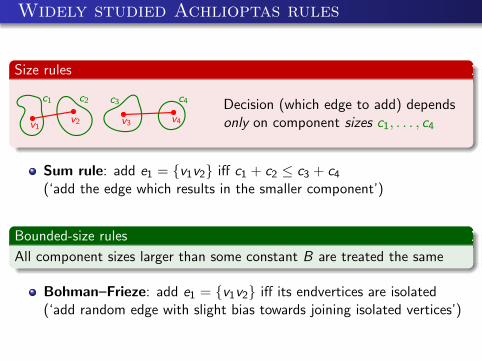
Widely studied Achlioptas rules

Size rules

v1v2 v3 v4

c1 c2 c3 c4 Decision (which edge to add) dependsonly on component sizes c1, . . . , c4

Sum rule: add e1 = {v1v2} iff c1 + c2 ≤ c3 + c4(‘add the edge which results in the smaller component’)

Bounded-size rules

All component sizes larger than some constant B are treated the same

Bohman–Frieze: add e1 = {v1v2} iff its endvertices are isolated(‘add random edge with slight bias towards joining isolated vertices’)

Previous work

Bounded-size rules (Spencer–Wormald, Bohman–Kravitz, Riordan–W.)

There is rule-dependent critical time tc > 0 such that, whp,

L1(tn) =

{

O(log n) if t < tc

Θ(n) if t > tc

Bohman–Frieze rule (Janson–Spencer)

There is rule-dependent c > 0 such that for constant ε > 0, whp,

L1(tcn + εn) ≈ cεn

Some further developments

Generalized Bohman–Frieze rules (Drmota–Kang–Panagiotou)

Critical window (Bhamidi–Budhiraja–Wang)

Other properties (Kang–Perkins–Spencer and Sen)

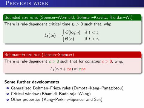
New Results for Bounded-Size Rules (1/4)

0

0.25

0.5

0.75

0.25 0.5 0.75 1

ER

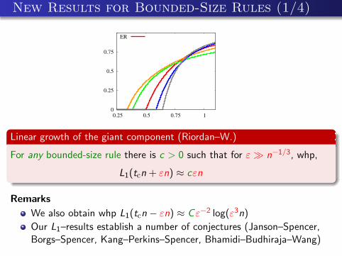
Linear growth of the giant component (Riordan–W.)

For any bounded-size rule there is c > 0 such that for ε ≫ n−1/3, whp,

L1(tcn + εn) ≈ cεn

Remarks

Same qualitative behaviour as in Erdos–Renyi process

Previous results: for constant ε > 0 and restricted class of rules

New Results for Bounded-Size Rules (1/4)

0

0.25

0.5

0.75

0.25 0.5 0.75 1

ER

Linear growth of the giant component (Riordan–W.)

For any bounded-size rule there is c > 0 such that for ε ≫ n−1/3, whp,

L1(tcn + εn) ≈ cεn

Remarks

We also obtain whp L1(tcn − εn) ≈ Cε−2 log(ε3n)

Our L1–results establish a number of conjectures (Janson–Spencer,Borgs–Spencer, Kang–Perkins–Spencer, Bhamidi–Budhiraja–Wang)

New Results for Bounded-Size Rules (2/4)

Size of the largest subcritical component (Riordan–W.)

For any bounded-size rule there is C > 0 such that for ε ≫ n−1/3, whp,

L1(tcn − εn) ≈ Cε−2 log(ε3n)

Remarks

Same qualitative form as in Erdos–Renyi process

Conjectured by Kang–Perkins–Spencer and Bhamidi–Budhiraja–Wang

Improves results of Bhamidi–Budhiraja–Wang and Sen

New Results for Bounded-Size Rules (3/4)

Number of vertices in small components (Riordan–W.)

For any bounded-size rule: as k → ∞ and ε → 0, we have

Nk(tcn ± εn) ≈ Ck−3/2e−(c+o(1))ε2kn

Remarks

Same qualitative form as in Erdos–Renyi process

Conjectured by Kang–Perkins–Spencer and Drmota–Kang–Panagiotou

Improves partial results of Drmota–Kang–Panagiotou

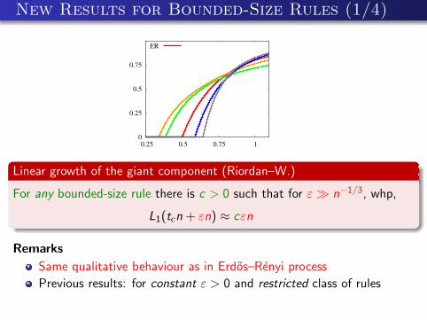
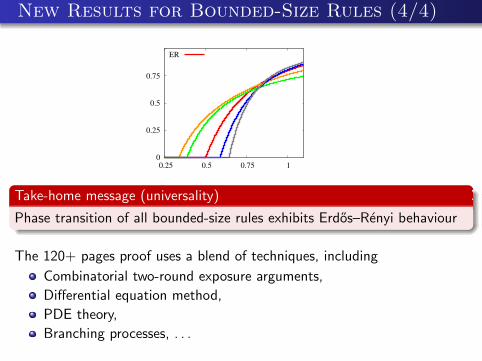
New Results for Bounded-Size Rules (4/4)

0

0.25

0.5

0.75

0.25 0.5 0.75 1

ER

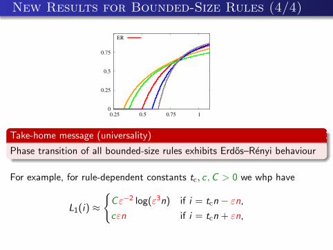
Take-home message (universality)

Phase transition of all bounded-size rules exhibits Erdos–Renyi behaviour

For example, for rule-dependent constants tc, c ,C > 0 we whp have

L1(i) ≈

{

Cε−2 log(ε3n) if i = tcn − εn,

cεn if i = tcn + εn,

New Results for Bounded-Size Rules (4/4)

0

0.25

0.5

0.75

0.25 0.5 0.75 1

ER

Take-home message (universality)

Phase transition of all bounded-size rules exhibits Erdos–Renyi behaviour

The 120+ pages proof uses a blend of techniques, including

Combinatorial two-round exposure arguments,

Differential equation method,

PDE theory,

Branching processes, . . .

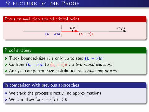
Structure of the Proof

Focus on evolution around critical point

stepstcn

(tc − σ)n (tc + ε)n

Proof strategy

Track bounded-size rule only up to step (tc − σ)n

Go from (tc − σ)n to (tc + ε)n via two-round exposure

Analyze component-size distribution via branching-process

In comparison with previous approaches

We track the process directly (no approximation)

We can allow for ε = ε(n) → 0

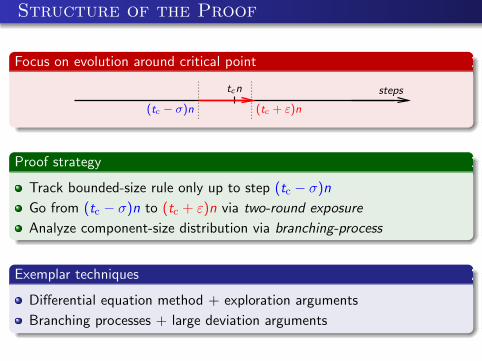
Structure of the Proof

Focus on evolution around critical point

stepstcn

(tc − σ)n (tc + ε)n

Proof strategy

Track bounded-size rule only up to step (tc − σ)n

Go from (tc − σ)n to (tc + ε)n via two-round exposure

Analyze component-size distribution via branching-process

Exemplar techniques

Differential equation method + exploration arguments

Branching processes + large deviation arguments

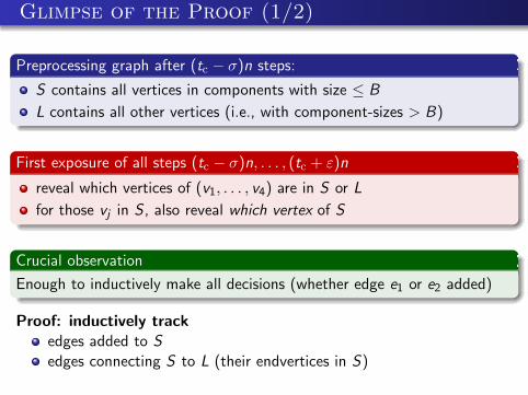
Glimpse of the Proof (1/2)

Preprocessing graph after (tc − σ)n steps:

S contains all vertices in components with size ≤ B

L contains all other vertices (i.e., with component-sizes > B)

First exposure of all steps (tc − σ)n, . . . , (tc + ε)n

reveal which vertices of (v1, . . . , v4) are in S or L

for those vj in S , also reveal which vertex of S

Crucial observation

Enough to inductively make all decisions (whether edge e1 or e2 added)

Proof: inductively track

edges added to S

edges connecting S to L (their endvertices in S)

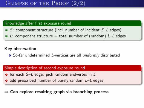
Glimpse of the Proof (2/2)

Knowledge after first exposure round

S : component structure (incl. number of incident S–L edges)

L: component structure + total number of (random) L–L edges

Key observation

So-far undetermined L-vertices are all uniformly distributed

Simple description of second exposure round

for each S–L edge: pick random endvertex in L

add prescribed number of purely random L–L edges

⇒ Can explore resulting graph via branching process

Some Difficulties

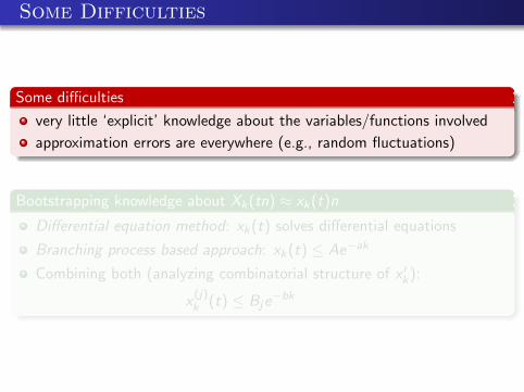
Some difficulties

very little ‘explicit’ knowledge about the variables/functions involved

approximation errors are everywhere (e.g., random fluctuations)

Bootstrapping knowledge about Xk(tn) ≈ xk(t)n

Differential equation method: xk(t) solves differential equations

Branching process based approach: xk(t) ≤ Ae−ak

Combining both (analyzing combinatorial structure of x ′k):

x(j)k (t) ≤ Bje

−bk

Summary

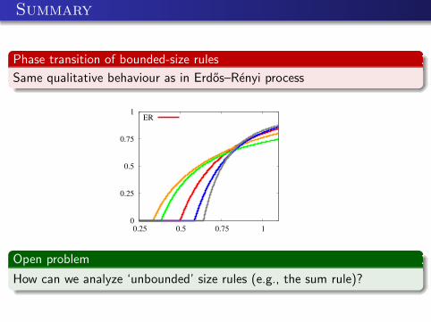
Phase transition of bounded-size rules

Same qualitative behaviour as in Erdos–Renyi process

0

0.25

0.5

0.75

1

0.25 0.5 0.75 1

ER

Open problem

How can we analyze ‘unbounded’ size rules (e.g., the sum rule)?