The nature of Dark Matter: -ray searches and the formation ...
285
UNIVERSIDAD DE GRANADA Tesis doctoral Julio 2009 The nature of Dark Matter: γ -ray searches and the formation of CDM halos [ PhD THESIS ] Miguel ´ Angel S´ anchez Conde Instituto de Astrof´ ısica de Andaluc´ ıa (CSIC) Memoria de Tesis presentada en la Universidad de Granada para optar al grado de Doctor en Astrof´ ısica Directores de tesis: Dr. Francisco Prada Mart´ ınez Prof. Mariano Moles Villamate
Transcript of The nature of Dark Matter: -ray searches and the formation ...

UNIVERSIDAD DE GRANADA
Tesis doctoralJulio 2009
The nature of Dark Matter:γ-ray searches and the formation of
CDM halos[ PhD THESIS ]
Miguel Angel Sanchez CondeInstituto de Astrofısica de Andalucıa (CSIC)
Memoria de Tesis
presentada en la Universidad de Granadapara optar al grado de Doctor en Astrofısica
Directores de tesis:
Dr. Francisco Prada MartınezProf. Mariano Moles Villamate

Editor: Editorial de la Universidad de GranadaAutor: Miguel Ángel Sánchez CondeD.L.: GR. 3517-2009ISBN: 978-84-692-6397-6

.

.
A ti, Raquel, por venir al mundo,y a ti, Marıa, por traerla.
Y a mis padres,por su apoyo y confianza ciegos.

.

.
Lo que sabemos es una gota de agua;lo que ignoramos es el oceano.
- Isaac Newton -
Una vez sentı el ansia
de una sed infinita.
- en Azul, de Ruben Darıo -
Una vez mas percibı ese raro contrasteentre las estrellas y nosotros.
La incalculable potencia del Cosmosacrecentaba misteriosamente la verdad
de nuestra breve chispa, y el brevee incierto destino de los hombres.
- en El hacedor de estrellas, de Olaf Stapledon -

.
Agradecimientos
Siempre quise ser astrofısico. Pese a los anos transcurridos, recuerdo con total nitidezaquella tarde de invierno del 91 en la que me compre mi primer telescopio, cuandoaun no era mas que un chiquillo de 11 anos. Aun me es posible rememorar la emocione ilusion que me embargaban cuando el Universo se iba desvelando ante mi tras aquelpequeno catalejo. He de reconocer que, afortunadamente, aun me llena el mismosentimiento, ahora sin duda mas maduro. Ha sido un largo camino hasta aquı y hay,por fortuna, mucho que agradecer y muchos a quienes agradecer.
En primer lugar, quisiera dar profundamente las gracias a mi director de tesis, PacoPrada. Ciertamente esta Tesis debe verse como producto de un trabajo compartidopor ambos a lo largo de estos anos. Su guıa en estos mis primeros y temblorosos pasosen la investigacion ha sido fundamental en la consecucion de las metas impuestasası como en el verdadero conocimiento de mis propias posibilidades. Su ambicion ymotivacion cientıficas han supuesto para mi un incentivo para llegar siempre mas alla,a cuestionarme con curiosidad cientıfica cada paso a dar y cada paso dado, a lograralcanzar objetivos a priori inalcanzables y que luego han demostrado ser tangibles.Gracias tambien por tu esfuerzo, dedicacion y preocupacion en moldearme como unbuen cientıfico.
No puedo dejar de acordarme tambien de todos aquellos colegas de profesion que alo largo de estos anos han sido fuente inagotable de conversacion cientıfica y pasioncompartida. Gracias especialmente a Mariano Moles por su apoyo y por creer en midesde el principio, ası como por compartir conmigo sus vastos conocimientos. Gra-cias tambien a mi asiduo colaborador en la distancia, Juan Betancort, por obligarmesiempre a ser particularmente metodico y conciso. Es a a el a quien debo por enteromis incursiones en la Cosmologıa mas teorica, pero tambien la confirmacion de mi feen el valor de los ideales. Mi agradecimiento tambien a todo mi grupo de trabajo en elIAA -Alberto, Antonio, Fabio, Hugo, Tono-, por ayudarme a respirar un ambiente detrabajo mas cientıfico todos los dıas, y en definitiva por compartir conmigo este duroaunque apasionante camino. No quiero pasar la oportunidad para agradecer igual-mente a todos aquellos amigos y colegas astrofısicos que me han hecho sentirme comouno mas del gremio siempre: Jurg Diemand, Mario Gomez, David Paneque, CarlosDelgado, Michele Doro, Radek Wojtak, Ewa Lokas, Elliott Bloom, Anatoly Klypin,Carlos Munoz, Gustavo Yepes, Daniel Kranich, Abelardo Moralejo. Tambien en el
viii
IAA he contado con la simpatıa y ayuda de varias personas que ya permaneceran enmi memoria como una pagina mas de esta Tesis: Antxon Alberdi, Benigno Cantero,Marıa Angeles Cortes, Emilio Garcıa, Isabel Marquez, Paco Navarro, Rafael Parra,Miguel A. Perez Torres.
Es cierto. Siempre quise ser astrofısico. Y sin duda lo soy gracias a mi familia, quecon una confianza sin lımites me alento siempre a perseguir mis mas alocados suenos.Esta Tesis no es sino la mejor muestra de ello. Mis padres, Antonio y Concha, siem-pre me apoyaron incondicionalmente a lo largo de todos estos anos, pese a que estapasion suponıa alejarme cientos de kilometros de ellos y ademas con destino incierto.Gracias por darme tanto y exigir tan poco, por moldearme como persona y esculpiren mi vuestra vision del mundo, por escuchar, por lanzaros al abismo conmigo sinsiquiera preguntar cuando hizo falta... Mi hermano mayor, Alaly, a quien con todaseguridad debo el hecho de haberme dedicado a esto de por vida, y con quien measome por vez primera a los secretos de la Astronomıa. Gracias por aquellas nochesinolvidables al raso entre las vinas, a un paso de casa pero en realidad muy lejos, entrelas estrellas. A mi hermano Jesus, que encontro sus propias estrellas en la musica,y que siempre ha significado para mi un soplo sincero de carino incondicional y unejemplo maestro de teson y valor ante lo que cada uno ansıa. Gracias tambien a miscunadas Marıa Jose y Txus, por brindar la felicidad a mis hermanos y formar partede nosotros. Definitivamente, los valores y el amor de mi familia han impregnadosiempre todo lo que he tocado y, por ende, esta Tesis necesariamente encierra unagran dosis del modo de hacer (y de ser) de los Sanchez Conde.
En el largo camino hasta aquı, no solo los misterios del Cosmos han ido desfilandoante mis ojos, sino tambien los de mi propia vida. Marıa, mi esposa y mejor con-fidente y amiga, supone para mi la mayor motivacion que es posible imaginar paracontinuar adelante. Sin duda es ella la luz que ilumina mi camino en esta vasta ytenebrosa oscuridad que es la propia existencia. Ella mejor que nadie sabe de mistriunfos y alegrıas, pero tambien de mis miedos y fracasos, derrotas y frecuentestropiezos, pues ha sido ella quien ha compartido mas de cerca conmigo cada subir ybajar de estos ultimos nueve anos. Ella ha sido el balsamo necesario para recuperarla serenidad y las ansias de seguir adelante en los momentos difıciles a lo largo deesta tesis. Gracias, carino, por estar siempre a mi lado. Y gracias tambien por darmea nuestra Raquel, que ya es la estrella mas brillante de nuestro cielo particular. Miagradecimiento tambien a mis suegros Miguel y Sole, y a mis cunados Miguel, Anay Alberto, por tratarme como uno mas de la familia y comprender el camino al queme veıa abocado por mi pasion por las estrellas.
Tambien tengo mucho que agradecer a aquellos buenos amigos que, por fortuna, mehan acompanado a lo largo de mi vida o en distintos momentos de ella. Mi ilusionha permanecido intacta todo este tiempo en buena medida gracias a muchos de mis
ix
amigos de Almendralejo, que con devocion ciega han seguido mi trayectoria y mehan aportado seguridad y confianza en mi mismo, ademas de entregarme su amistadmas profunda y sincera: Moi, Leandro, Julio, Paco, Jesus, Mario, Lucky, Martın,Zaca, los hermanos Jareno. Tambien Agustın, Alex, Belen, Chovis, Diego, Jose,Juan, Marcos, Merchan, Paco Melado, Patricia, Velarde... ¡Como olvidar aquellasnoches en el Puente de las Peras (que no de la Espera) trazando nuestros planes decomernos el mundo a la unica luz de las estrellas! Bien sabeis muchos de vosotrosque este era el mas preciado para mi... Tambien mis tres anos de estudios en Badajozme proporcionaron amigos que aun hoy siguen en mi vida y a los que agradezcoenormemente su apoyo continuo y amistad: Pedro, Vıctor, Juli, Merche, Vicente,Lidia, Miguel A y B, Noelia, Rosalıa, Raquel, Luis, Juampe... En Badajoz tambienconocı a Antonio, con el que ya entonces compartıa aficiones y conocimientos, ycon el que luego compartirıa dıa a dıa, y como una y carne, todo sueno y todoanhelo. Fue con el con quien me embarque en mi aventura canaria, en nuestra mutuadeterminacion por llegar a ser lo que ahora somos (esto es, ni mas ni menos quelo que siempre quisimos ser). Gracias por mantenerte siempre cerca. De esa etapauniversitaria canaria, rodeado de mar y a tres meses de casa, debo agradecer que eldestino pusiera en mi camino en especial a Luis, con su inagotable vitalidad, a Placido,con sus ferreos ideales, a Charly, Darıo (en aquella epoca el Peludo), Omaira, Mar,Alicia, Manolo, los dos Jorge, Jairo, Ruben, Teo, Susi, David, Javi, Rebeca. Con elloscompartı aquellos anos inolvidables al pie del Teide, y sobre el tambien, y muchosamaneceres sobre el mar. El destino burlon ha vuelto a juntarnos a varios de nosotrosen Granada, donde nuestra amistad ha madurado y se ha estrechado aun mas. ElTriunvirato de Cuatro es buena prueba de ello: Charly, Dani, Darıo han sido mismas leales amigos y companeros de aventuras y desventuras durante todos los dıasde la Tesis. Gracias por aguantarme incluso en los peores dıas, por poner siempreun toque de humor a todo y por salir en mi auxilio cuando lo necesitaba. Graciasen Granada tambien a todos los doctorandos con los que he coincidido, en especial aAntonio (de Ugarte), Antonio (Garcıa), Diego, Gabriela, Geli, Marcos, Marta, Meme,Nieves, Paco, Silbia y Vıctor. Hay luz al final del tunel, chicos. Y gracias a la pena defutbito, por esos momentos de relax y desconexion. Por ultimo, no quisiera olvidarmede aquellos que, aun no siendo ni de Almendralejo, Badajoz, Tenerife o Granada, hanjugado un papel esencial en esta aficion mıa primero y profesion despues. Mil graciasespecialmente a Paco Rica, al que (a pesar de ser de Merida) me une ya una vieja ysolida amistad y una gran admiracion mutua. Gracias por creer siempre en mi... Ygracias tambien a los colombianos Rafa y Esteban, con quienes compartı mi primeraaventura americana y mi primer contacto real con la investigacion en la NASA.
He de agradecer aquı tambien a aquellos lugares que han sido especialmente impor-tantes para mi, cada uno por sus propios motivos, y cuya simple evocacion siempre hasupuesto una motivacion extra para conseguir aquello que me propusiera. Entre ellosdestacare a Extremadura, y en particular Almendralejo, con sus campos de vinas yolivos, su cielo azul inmenso y sus gentes, y que sin duda ha dejado su huella en mi
x
forma de ser; el Rıo Guadiana, en cuyas orillas encontre a la mujer de mi vida; LaPalma y sus telescopios recortados sobre el fondo estrellado; ya mas cercanos en eltiempo y el espacio, Granada y sus tapas, el Enano Rojo, el Rodri y el Romero, igual-mente importantes en algunos momentos para conseguir acabar la Tesis. Y, desdeluego, por encima de todo, gracias a la ventana por la que nos asomamos al Universo,y al Universo mismo, por ser tan absolutamente maravilloso y fascinante.
Aun conservo aquel pequeno telescopio con el que empece a escrudinar el cielo en miinfancia. Cada vez que vuelvo a casa (que por siempre sera Almendralejo), su visionme reconforta y me ayuda a recordar, y no olvidar, de donde vengo. Me reconfortaigualmente sentir dentro de mi como mi vieja pasion por desvelar los misterios delCosmos no ha disminuido en absoluto; al contrario, puedo sentirla mas viva quenunca corriendo por mis venas y aguantando en pie mis huesos. Sirva de muestraesta Tesis. A dıa de hoy, tengo claro que esto tambien es ası gracias a vosotros, atodos aquellos que habeis hecho que estas lıneas de agradecimiento sean tan extensas,porque como ya dije al principio, hay mucho, mucho, de lo que agradecer y a quienagradecer. A buen seguro, no hubiera llegado tan lejos sin vuestro afecto y companıa.Por tanto, es mi deseo que penseis en esta Tesis tambien, al menos en parte, comoalgo genuinamente vuestro.
Resumen
En esta Tesis Doctoral, la principal lınea de investigacion se ha centrado en la com-prension de la naturaleza de la Materia Oscura. Con el objetivo de abordar de formaadecuada dicho problema cientıfico y arrojar luz sobre el mismo, he usado differentesaproximaciones, tanto observacionales como teoricas. A lo largo de estas lıneas re-sumire las que han sido mis mas notables contribuciones en el campo.
Desde el comienzo de mi Tesis, he dedicado un gran esfuerzo para entender comose forman y evolucionan los halos de Materia Oscura Frıa (o CDM, de sus siglas eningles) en el marco del modelo cosmologico estandar. En particular, en un primertrabajo me centre en la compresion y caracterizacion de las partes mas externas dedichos halos de CDM, mas alla del radio virial. Este trabajo se presenta en detalleen el Capıtulo 2, y esta basado en el uso del modelo de Colapso Esferico (o SIM,de sus siglas en ingles) sin cruce de capas. En el mismo Capıtulo describo ademasel marco teorico que permite llevar a cabo la comparacion entre las predicciones dedicho modelo con los resultados obtenidos mediante simulaciones cosmologicas de N-cuerpos. La conclusion principal de este trabajo es que SIM, a pesar de su simplicidad,es capaz de proporcionar predicciones detalladas que estan en buen acuerdo con lassimulaciones al menos a grandes distancias del centro del halo.
Todavıa relacionado con lo anterior, comence un ambicioso trabajo con el objetivo deestudiar la formacion y evolucion de halos de CDM haciendo uso de un modelo SIMmejorado, esta vez incluyendo el cruce de capas en el formalismo. En el Capıtulo 3presento el marco teorico necesario para manejar dicho efecto de forma apropiada,que ademas no involucra el uso de ningun invariante adiabatico y que esta basado enel seguimiento numerico, en el tiempo, de una capa individual de materia de las quecomponen el halo. Este trabajo no incluye, por el momento, ni momento angular nivelocidades de dispersion.
Dentro de este marco teorico -que llame Spherical Shell Tracker (SST), y que podrıaser traducido como Rastreador de Capas Esfericas - estudie en detalle la evoluciondel halo, obteniendo por ejemplo el momento exacto en el cual ocurre el primer crucede capas, los valores exactos de tiempo y radio para los cuales se alcanza un ciertovalor de contraste de densidad lineal y real, δl y δ respectivamente, el valor de ambos

xii
contrastes de densidad en el momento en el cual se produce el colapso de acuerdo almodelo SIM sin cruce de capas, o la relacion entre los contrastes de densidad lineal yreal, esto es, la funcion δl(δ). Asimismo, investigue la dependencia de la evolucion delhalo con su masa virial, con la fraccion de masa considerada respecto a dicha masavirial, y con la cosmologıa para los casos de un Universo Einstein-deSitter y uno conΩm=0.3 y ΩΛ=0.7. Lo que encontre es que los resultados obtenidos son muy sensi-bles a la variacion de la masa virial o a la fraccion de masa virial que se considere.Sin embargo, obtuve una dependencia totalmente despreciable con la cosmologıa.Por otro lado, en el mismo Capıtulo muestro que el efecto del cruce de capas juegaun papel fundamental en la forma en que el halo evoluciona y alcanza el equilibriovirial y su estabilizacion en radio. Ademas, discuto como los valores que se adoptancomunmente en la literatura para los contrastes de densidad lineal y real podrıan noser del todo precisos. Este hecho tiene importantes implicaciones por ejemplo parauna correcta definicion de masa y radio viriales en el halo.
En esta Tesis, la mayor parte del trabajo realizado respecto a la deteccion de materiaoscura, y en particular todo el trabajo que concierne a la busqueda de aniquilacionde dicha materia, se centra unicamente en el rango de los rayos gamma. Esto quieredecir que no se han explorado ni la antimateria ni los neutrinos como otros posiblesproductos de la aniquilacion. Pero, ¿por que rayos gamma y no otras longitudes deonda? El punto esencial es que la escala de energıas de los productos de aniquilacionviene determinada por la masa de la partıculas que conforman la materia oscura,puesto que son estas las que tıpicamente se llevan una gran fraccion de la energıade aniquilacion disponible. Dado que las partıculas que se barajan mas seriamentecomo candidatas a formar la materia oscura, como el neutralino, se espera que tenganmasas del orden de ∼GeV-TeV, esto explica que las busquedas de materia oscura selleven a cabo especialmente en la banda energetica de los rayos gamma. Por otro lado,ademas de centrarme en dicha banda espectral, he invertido la mayor parte de misesfuerzos de busqueda de materia oscura en un escenario de aniquilacion en el cualel neutralino es el largamente buscado WIMP (del ingles Weakly Interacting MassiveParticle, o en espanol partıcula masiva debilmente interactuante) y que ademas existeen suficientes cantidades como para dar cuenta de la totalidad de la materia oscurano barionica en el Universo. Este trabajo se presenta en los Capıtulos 4, 6, 8, 9. Laexcepcion es el Capıtulo 5, en el cual se abordan y estudian en detalle las perspectivasde deteccion para otro candidato posible (el axion), tambien en rayos gamma. En estecaso, el metodo usado para la busqueda de dicha partıcula se basa en las oscilacionesentre fotones y axiones predichas por la fısica de partıculas.
Siempre que fue posible, combine tanto teorıa como observaciones (esto ultimo gra-cias a mi participacion en la Colaboracion MAGIC). Mas en detalle, y primero enrelacion a mi aproximacion teorica al problema, he llevado a cabo calculos precisosdel flujo de aniquilacion de materia oscura para los candidatos astrofısicos mas pro-metedores. En particular, en el Capıtulo 4 se presentan las predicciones de flujo ası

xiii
como las perspectivas de deteccion de la galaxia esferoidal Draco para un telescopioIACT tıpico y para el satelite Fermi. Los resultados de este trabajo han ayudado acomprender el verdadero potencial de Draco como buen candidato para las busquedasde materia oscura ası como las posibilidades reales de deteccion de aniquilacion demateria oscura en dicha enana por parte de los IACTs actuales.
En la vertiente observacional, y como miembro activo de la Colaboracion MAGIC yde su Grupo de Trabajo de Materia Oscura, he estado involucrado durante mi Tesisen las campanas observacionales llevadas a cabo con dicho telescopio para la deteccionde materia oscura en dos galaxias enanas: Draco (Capıtulo 8) y Willman 1 (Capıtulo9). No se encontro senal gamma alguna en ninguna de estas observaciones, y loslımites superiores impuestos a un posible flujo gamma no detectado parecen estar to-davıa lejos de una posible deteccion, al menos de acuerdo a las predicciones teoricasmas realistas. Tampoco fue posible la exclusion de alguna porcion de la region per-mitida del espacio de parametros; sin embargo, estas observaciones han representadoel primer intento serio de busqueda de materia oscura en galaxias enanas satelitesde la Vıa Lactea con IACTs, y los lımites superiores al flujo permitieron excluir almenos un alto flujo de aniquilacion (propuesto por algunos trabajos en la literatura).Finalmente, ni que decir tiene que las incertidumbres en las predicciones de flujo sonenormes, por lo que en cualquier caso estas observaciones con IACTs no son soloadecuadas sino tambien totalmente necesarias.
Ademas de MAGIC, tambien he invertido un esfuerzo muy significativo en el experi-mento de I+D conocido como GAW (de las siglas en ingles de Gamma Air Watch) conel objetivo de llegar a hacerlo una realidad. GAW es un conjunto de 3 telescopios contecnologıa IACT que estara situado en el Observatorio de Calar Alto, y que operarapor encima de los ∼700 GeV en un futuro proximo. El principal objetivo de GAWes examinar la viabilidad de una nueva generacion de IACTs que combinen una altasensibilidad con un gran campo de vision. En particular, mi trabajo en GAW se hacentrado en la definicion de los objetivos cientıficos del instrumento ası como en lajustificacion de la necesidad de semejante experimento. El Capıtulo 6 se dedica porentero a describir mis principales contribuciones cientıficas dentro de la ColaboracionGAW.
En un intento de explorar otros escenarios posibles en los cuales la partıcula queconstituye la materia oscura es diferente del neutralino, he investigado tambien elpapel que los axiones ultraligeros podrıan desempenar como buenos candidatos. Losresultados, que presento en el Capıtulo 5, podrıan ser cruciales para los experimentosactuales que operan en rayos gamma y en especial para una correcta interpretacionde sus observaciones. Si dichas partıculas existen y tienen masas ∼10−10 eV, podrıaocurrir que se dieran oscilaciones foton/axion en presencia de campos magneticos,tales como los que se espera que existan en los Nucleos de Galaxias Activas (o AGNs,de sus siglas en ingles) o en el Medio Intergalactico. Esto conllevarıa una distorsion
xiv
significativa en el espectro de aquellas fuentes astrofısicas emisoras de rayos gamma.Por tanto, en dicho trabajo explore de un lado las perspectivas de deteccion de talesdistorsiones espectrales, y de otro propuse la que podrıa representar la mejor estrate-gia observacional. Dicha estrategia requerirıa de un esfuerzo conjunto entre Fermi eIACTs, ası como de la observacion con dichos telescopios de AGNs distantes (z > 0.1).Ademas, en el mismo Capıtulo tambien muestro como el papel de los axiones podrıaser crıtico para una correcta interpretacion y modelaje de la Luz de Fondo Extra-galactica (mas conocida como EBL, de sus siglas en ingles).
Finalmente, los Capıtulos 10 y 11 se dedican, respectivamente, a presentar las prin-cipales conclusiones alcanzadas en la Tesis y a exponer brevemente el trabajo que seplanea desarrollar en un futuro.
Para concluir, serıa natural preguntarse el por que de este enorme interes en labusqueda indirecta de materia oscura en la banda gamma precisamente ahora, alcomienzo del siglo XXI (y especialmente teniendo en cuenta que este tipo de busquedasya fueron propuestas hace 25 anos). Hay buenas razones para ser particularmenteoptimistas en el presente: los experimentos actuales que operan en rayos gamma, talescomo los nuevos IACTs y el satelite Fermi de la NASA, estan por vez primera alcan-zando sensibilidades suficientemente buenas como para ser capaces de poner a pruebaalgunos de los escenarios permitidos y preferidos por la comunidad astrofısica y departıculas (esto es, aquellos que obedecen las restricciones impuestas por las observa-ciones del satelite WMAP, aquellos que hacen uso de perfiles de densidad de materiaoscura bien motivados fısicamente, y aquellos que se centran en la Supersimetrıa).Se espera que la situacion mejore aun mas con la entrada en funcionamiento de lanueva generacion de telescopios IACT en el futuro cercano (CTA, AGIS...). La ven-tana espectral de los rayos gamma acaba de abrirse a nuestros descubrimientos, ysin duda una revolucion en el cielo GeV-TeV esta en ciernes. Es definitivamente elmomento idoneo para las busquedas de materia oscura en rayos gamma.
Summary
In this Thesis, the main research activities are focused on the understanding of thenature of the Dark Matter (DM). In order to shed some light on this challengingtopic, I used different both theoretical and observational approaches. Below I sum-marize my work contribution to this field.
Since the beginning of my Thesis, a large effort was devoted to understanding howCold DM halos form and evolve within the cosmological standard model. Indeed, Ifocused my first work on the understanding and characterization of the outskirts ofCDM halos, i.e. well beyond the virial radius. This work is presented in detail inChapter 2, and is based in the spherical infall model (SIM) without shell crossing.In addition, I also describe in the same Chapter the framework that allows for acomparison of these predictions with the results obtained from N-body cosmologicalsimulations. The main conclusion of this work is that SIM, despite its simplicity, iscapable to provide detailed predictions that are in good agreement with simulationsat least at those large radii.
An ambitious work was also started to study the formation and evolution of coldDM halos by means of an improved SIM with shell-crossing. In Chapter 3, I presenta framework to tackle this effect properly, that does not involve to use any adiabaticinvariant, and that is based on the numerical follow-up of an individual shell of matterwith time. This work does not include, by the moment, neither angular momentumnor velocity dispersion.
Within this framework -which I named as the Spherical Shell Tracker (SST )- Istudied in detail the evolution of a halo, e.g. obtaining the exact moment when thefirst shell-crossing occurs, the exact values of time and radius for a given value ofthe linear or actual density contrasts, δl and δ respectively, the value of both densitycontrasts when the collapse occurs according to the standard SIM, or the relationbetween the linear and actual density contrasts, i.e., the function δl(δ). I investigatedthe dependence of the evolution with the virial mass, with the fraction consideredrespect to this virial mass, and with the cosmology for the cases of Einstein-deSitterand Ωm = 0.3, ΩΛ = 0.7 cosmologies. What I found is that the results are very sen-sible to a variation of the virial mass or the fraction of virial mass that we consider.
xvi
However, I obtain a negligible dependence with the cosmology. Furthermore, I showthat the effect of shell-crossing plays a crucial role in the way that the halo evolvesand reaches the virial equilibrium and the stabilization in radius. Indeed, the valuescurrently adopted in the literature for the actual density contrast at the moment ofvirialization may not be accurate enough. This fact has important implications e.g.in the definition of a virial mass and a virial radius for the halo.
In this Thesis, most of the work related to DM detectability, and in particular allthe work done concerning DM annihilations, is focused only on γ-ray searches. Thismeans that neither antimatter nor neutrinos as other possible annihilation productswere explored. But why γ-rays and not other wavelenghts? The keypoint is thatthe energy scale of the annihilation products is determined by the mass of the DMparticles, as they typically carry a relatively large fraction of the available annihila-tion energy. Since the preferred DM candidates like the neutralino are expected tohave masses of the order of ∼GeV-TeV, this explains that DM searches are speciallyperformed in the γ-ray energy band. Furthermore, I centered most of my DM searchefforts in a DM annihilation scenario where the neutralino is the long-searched forWIMP that exists in sufficient quantities to constitute the totality of the non-baryonicDM in the Universe. This work is presented in Chapters 4, 6, 8, 9. The exceptionis Chapter 5, in which the DM detection prospects for another plausible candidate(the axion) was studied in detail, also in γ-rays. In this case, predicted photon/axionmixings rather than self-annihilations are the vehicle used in the search of the DMparticle.
Whenever possible, I combined both theory and observations, the latter beingpossible thanks to my participation in the MAGIC Collaboration. More in detail, andfirst regarding the theoretical approach, I carefully calculated the DM annihilationflux for the most promising candidates. In particular, flux predictions as well asdetection prospects for a typical IACT and for the Fermi satellite for the Draco dwarfspheroidal galaxy are presented in Chapter 4. The results helped to understand thereal potential of Draco as a good DM candidate and the real capabilities of the currentIACTs in the search for DM in this dwarf. In the same Chapter, I also stress thecrucial role of the angular resolution of the instrument in a correct interpretation ofthe observational data in the context of DM searches.
In the observational side, and as a member of the MAGIC Collaboration andactive member of the MAGIC DM Working Group, I have been involved in the ob-servational campaigns carried out for two dwarf galaxies: Draco (Chapter 8) andWillman 1 (Chapter 9). No gamma signal was found in any of these observations,and the derived upper limits seem to be still far from a successful detection accord-ing to theoretical predictions. An exclusion of some portion of the allowed region inthe parameter space is not possible either; however, these observations representedthe first serious attempt of DM searches in dwarf galaxy satellites carried out by anIACT, and the upper limits excluded a large annihilation signal at least (as claimed
xvii
by some works in the literature). Finally, needless to say that the uncertainties inthe flux predictions are huge, so IACT observations are encouraged in any case.
In addition to MAGIC, I also invested a significant effort in order to launch theGAW R&D experiment. GAW is an array of 3 IACTs planned to be located at CalarAlto Observatory, that will operate above ∼700 GeV in the near future. The mainobjective of GAW is to test the feasibility of a new generation of IACTs, which com-bine high sensitivity with a large Field of View. I worked on the definition of thescience objectives of the instrument as well as in the justification of such an experi-ment. Chapter 6 is devoted to GAW and to describe my main scientific contributionsinside the GAW Collaboration.
In an attempt to find and explore other plausible DM scenarios where the DMparticle could be different from the neutralino, I have also investigated the possiblerole of ultra-light axions as DM candidates. The results, presented in Chapter 5,could be crucial for current gamma-ray experiments and observations. If these parti-cles exist and have masses ∼10−10 eV, photon/axion oscillations might occur in thepresence of magnetic fields, such as those expected to be present in AGNs or in theIntergalactic Medium. This would lead to a distortion in the spectra of gamma-raysources significantly, depending on source distance and the involved magnetic fields.Therefore, I did explore the detection prospects and propose the most appropriateobservational strategy. This strategy would require a joint effort of Fermi and IACTslooking at distant AGNs (z > 0.1). Moreover, I show that axions might be critical ina correct interpretation and modeling of the Extragalactic Background Light as well.
Main conclusions of the work presented in this Thesis and future work is presentedin Chapters 10 and 11 respectively.
To conclude, it would be natural to ask why this huge interest on indirect γ DMsearches precisely now, at the beginning of the 21st Century (specially taking intoaccount that these kind of searches were proposed at least 25 years ago). There aregood reasons to be specially optimistic at present: current γ-ray experiments likeIACTs and Fermi are reaching for the first time sensitivities good enough to be ableto test some of the allowed and preferred scenarios (i.e. obeying WMAP constraints,taking well-motivated DM density profiles and using SUSY). The situation is expectedto be even better when new generation telescopes enter in operation in the near future(CTA, AGIS...). The γ-ray energy window has just opened to our discoveries, and arevolution in the GeV-TeV sky is on the way. It is time for γ-ray DM searches.

.
Index
Agradecimientos vii
Resumen xi
Summary xv
1 Introduction: the Dark Matter challenge 1
1.1 Observational evidences for Dark Matter . . . . . . . . . . . . . . . . 1
1.2 The ΛCDM paradigm . . . . . . . . . . . . . . . . . . . . . . . . . . . 5
1.2.1 A brief mathematical description of the model . . . . . . . . . 6
1.2.2 Cosmological parameters . . . . . . . . . . . . . . . . . . . . . 8
1.2.3 Structure formation . . . . . . . . . . . . . . . . . . . . . . . . 11
1.2.4 Problems to be solved. Any alternative scenario? . . . . . . . 12
1.3 Dark Matter and N-body cosmological simulations . . . . . . . . . . . 16
1.4 What is Dark Matter made of? . . . . . . . . . . . . . . . . . . . . . 19
1.4.1 Barionic Dark Matter . . . . . . . . . . . . . . . . . . . . . . . 20
1.4.2 Non-baryonic Dark Matter particle candidates . . . . . . . . . 21
1.5 Dark Matter searches . . . . . . . . . . . . . . . . . . . . . . . . . . . 24
1.5.1 Direct detection . . . . . . . . . . . . . . . . . . . . . . . . . . 25
1.5.2 Indirect detection and the γ-ray connection . . . . . . . . . . 27
1.5.3 The importance of γ-ray DM searches . . . . . . . . . . . . . . 28
1.6 The γ-ray energy window: IACTs, Fermi and future instruments . . . 29
1.6.1 Gamma-ray astrophysics in a nutshell . . . . . . . . . . . . . . 29
1.6.2 The imaging atmospheric Cherenkov technique. Present IACTs 33
1.6.3 The Fermi satellite . . . . . . . . . . . . . . . . . . . . . . . . 37
1.6.4 Planned instruments for the near future . . . . . . . . . . . . 42
1.7 Present status of γ-ray Dark Matter searches and hints of detection . 43
References . . . . . . . . . . . . . . . . . . . . . . . . . . . . . . . . . 51
xx
I Formation and evolution of CDM halos 61
2 Theoretical predictions for the outskirts of DM halos 63
2.1 Introduction . . . . . . . . . . . . . . . . . . . . . . . . . . . . . . . . 63
2.2 The typical density profile of Dark Matter Halos . . . . . . . . . . . . 66
2.3 The Probability Distribution, P (δ, r). Most Probable and Mean Profiles 69
2.4 Comparison with N-body simulations . . . . . . . . . . . . . . . . . . 73
2.5 Improving P (δ, r) . . . . . . . . . . . . . . . . . . . . . . . . . . . . . 79
2.6 Final remarks . . . . . . . . . . . . . . . . . . . . . . . . . . . . . . . 82
References . . . . . . . . . . . . . . . . . . . . . . . . . . . . . . . . . . . . 84
3 The spherical collapse model with shell-crossing 87
3.1 Introduction . . . . . . . . . . . . . . . . . . . . . . . . . . . . . . . . 87
3.2 The Spherical Shell Tracker Framework . . . . . . . . . . . . . . . . . 91
3.3 The formalism . . . . . . . . . . . . . . . . . . . . . . . . . . . . . . . 91
3.4 The algorithm . . . . . . . . . . . . . . . . . . . . . . . . . . . . . . . 95
3.5 The evolution of the halo: effect of shell-crossing . . . . . . . . . . . . 98
3.6 Stabilization and Virialization . . . . . . . . . . . . . . . . . . . . . . 103
3.7 Stabilization . . . . . . . . . . . . . . . . . . . . . . . . . . . . . . . . 105
3.8 Virialization . . . . . . . . . . . . . . . . . . . . . . . . . . . . . . . . 106
3.9 Comparison between stabilization and virialization: general consider-ations . . . . . . . . . . . . . . . . . . . . . . . . . . . . . . . . . . . 107
3.10 Summary and future work . . . . . . . . . . . . . . . . . . . . . . . . 110
References . . . . . . . . . . . . . . . . . . . . . . . . . . . . . . . . . . . . 112
II γ-ray Dark Matter searches: detection prospects 115
4 Dark matter annihilation in Draco and detection prospects 117
4.1 Introduction . . . . . . . . . . . . . . . . . . . . . . . . . . . . . . . . 117
4.2 The γ-ray flux in IACTs . . . . . . . . . . . . . . . . . . . . . . . . . 120
4.2.1 Particle physics: the fSUSY parameter . . . . . . . . . . . . . 120
4.2.2 Astrophysics: the U(Ψ0) parameter . . . . . . . . . . . . . . . 126
4.3 Dark matter distribution in Draco . . . . . . . . . . . . . . . . . . . . 127
4.4 Draco gamma ray flux profiles . . . . . . . . . . . . . . . . . . . . . . 130
4.5 Detection prospects for some current or planned experiments . . . . . 134
4.5.1 Flux profile detection . . . . . . . . . . . . . . . . . . . . . . . 134
4.5.2 Excess signal detection . . . . . . . . . . . . . . . . . . . . . . 135
4.6 Conclusions . . . . . . . . . . . . . . . . . . . . . . . . . . . . . . . . 138
References . . . . . . . . . . . . . . . . . . . . . . . . . . . . . . . . . . . . 143

xxi
5 Hints of the existence of ALPs from the γ-ray spectra of cosmologicalsources 147
5.1 Introduction . . . . . . . . . . . . . . . . . . . . . . . . . . . . . . . . 148
5.2 The formalism . . . . . . . . . . . . . . . . . . . . . . . . . . . . . . . 150
5.2.1 Mixing inside and near the source . . . . . . . . . . . . . . . . 151
5.2.2 Mixing in the IGMFs . . . . . . . . . . . . . . . . . . . . . . . 154
5.3 Results . . . . . . . . . . . . . . . . . . . . . . . . . . . . . . . . . . . 159
5.3.1 Photon/axion oscillation in our framework . . . . . . . . . . . 160
5.3.2 The impact of changing B . . . . . . . . . . . . . . . . . . . . 165
5.3.3 The impact of using the smallest coupling constant . . . . . . 167
5.4 Detection prospects for Fermi and IACTs . . . . . . . . . . . . . . . . 169
5.5 Conclusions . . . . . . . . . . . . . . . . . . . . . . . . . . . . . . . . 173
References . . . . . . . . . . . . . . . . . . . . . . . . . . . . . . . . . . . . 175
6 DM searches with GAW 179
6.1 GAW: an R&D experiment in Calar Alto . . . . . . . . . . . . . . . . 179
6.1.1 Scientific case . . . . . . . . . . . . . . . . . . . . . . . . . . . 180
6.1.2 Main technical characteristics . . . . . . . . . . . . . . . . . . 182
6.2 The GAW strategy to look for DM in the Milky Way . . . . . . . . . 187
6.3 The GAW Search for Nearby Earth-size Dark Matter Micro-Halos . . 191
6.4 GAW Prospects for Dark Matter detection from IMBHs . . . . . . . . 193
References . . . . . . . . . . . . . . . . . . . . . . . . . . . . . . . . . . . . 195
III DM searches with the MAGIC-I telescope 197
7 An overview of the MAGIC telescopes 199
7.1 MAGIC: the lowest energy threshold of current IACTs . . . . . . . . 200
7.2 Main technical characteristics . . . . . . . . . . . . . . . . . . . . . . 202
7.3 The MAGIC-II stereoscopic system . . . . . . . . . . . . . . . . . . . 205
7.4 Participation of the IAA-CSIC group in MAGIC . . . . . . . . . . . . 206
References . . . . . . . . . . . . . . . . . . . . . . . . . . . . . . . . . . . . 209
8 Dark Matter searches in the Draco dSph with MAGIC 211
8.1 Introduction . . . . . . . . . . . . . . . . . . . . . . . . . . . . . . . . 211
8.2 Expected γ-Ray Flux From Neutralino Self-Annihilation . . . . . . . 212
8.3 Observation of Draco and Analysis . . . . . . . . . . . . . . . . . . . 215
8.4 Results . . . . . . . . . . . . . . . . . . . . . . . . . . . . . . . . . . . 215
8.5 Conclusions . . . . . . . . . . . . . . . . . . . . . . . . . . . . . . . . 218
xxii
9 Dark Matter searches in the Willman 1 dSph with MAGIC 2219.1 Introduction . . . . . . . . . . . . . . . . . . . . . . . . . . . . . . . . 2219.2 Willman 1 . . . . . . . . . . . . . . . . . . . . . . . . . . . . . . . . . 2239.3 Theoretical modeling of the gamma-ray emission from Willman 1 . . 224
9.3.1 Astrophysical Factor . . . . . . . . . . . . . . . . . . . . . . . 2249.3.2 Particle Physics Factor . . . . . . . . . . . . . . . . . . . . . . 225
9.4 MAGIC data . . . . . . . . . . . . . . . . . . . . . . . . . . . . . . . 2279.5 Results and Discussion . . . . . . . . . . . . . . . . . . . . . . . . . . 2289.6 Conclusion . . . . . . . . . . . . . . . . . . . . . . . . . . . . . . . . . 231References . . . . . . . . . . . . . . . . . . . . . . . . . . . . . . . . . . . . 232
IV Conclusions and future work 235
10 Conclusions 237
11 Future work 241
A Appendix 245A.1 The Formalism in the ΛCDM cosmology . . . . . . . . . . . . . . . . 245A.2 Results obtained for stabilization and virialization . . . . . . . . . . . 247
B Publications 251
List of Tables
2.1 Artificial cut-off for P (δ, r) . . . . . . . . . . . . . . . . . . . . . . . . . 72
2.2 Comparison between the simulated mean halo density profile and the theo-
retical predictions from the spherical collapse model for the mass < M >=
3 × 10¹²h−1 M⊙. . . . . . . . . . . . . . . . . . . . . . . . . . . . . . . 74
2.3 The isolated mean halo density profile for the mass < M >= 3×10¹²h−1 M⊙.
The symbols are the same as Table 2.4. . . . . . . . . . . . . . . . . . . 76
3.1 Values of b and Q neccesary to use the approximation for δ0 given by (3.14). 94
3.2 Linear (δl) and actual (δ) density contrast values related to some important
moments in the evolution of a halo with a virial mass Mvir = 3×10¹²h−1 M⊙and for the Einstein-deSitter and Ωm = 0.3, ΩΛ = 0.7 cosmologies . . . . . 100
3.3 Linear (δl) and actual (δ) density contrast values related to some important
moments in the evolution of a halo for three different virial masses (Mvir =
6.5 × 10¹⁰h−1 M⊙, Mvir = 3 × 10¹²h−1 M⊙ and Mvir = 5 × 10¹⁴h−1 M⊙)
and two different cosmologies (Einstein-deSitter and Ωm = 0.3, ΩΛ = 0.7).
A value of Mfrac = 0.5 was set in all the cases . . . . . . . . . . . . . . . 101
3.4 Degree of agreement with the virial theorem (VIR) and the moment of
stabilization (STA) for two moments of evolution, VIR1 and VIR2, and for
different values of Mfrac and two cosmologies. A virial mass of Mvir =
3 × 10¹² h−1 M⊙ was used in all the cases . . . . . . . . . . . . . . . . . 108
3.5 Degree of agreement with the virial theorem (VIR) and the moment of
stabilization (STA) for two moments of evolution, VIR1 and VIR2, and for
three different virial masses and two cosmologies. A value of Mfrac = 0.5
was used in all the cases . . . . . . . . . . . . . . . . . . . . . . . . . . 109
4.1 Best-fitting parameters of the two-component models for the DM profiles
with a cusp and a core for Draco . . . . . . . . . . . . . . . . . . . . . . 128
4.2 DM density profile parameters obtained for Draco . . . . . . . . . . . . . 131
4.3 Prospects of an excess signal detection for MAGIC, Fermi and GAW . . . 138

xxiv LIST OF TABLES
5.1 Maximum attenuations due to photon/axion oscillations in the source ob-
tained for different sizes of the region where the magnetic field is confined
and different lengths for the coherent domains. The B field strength used
is 1.5 G . . . . . . . . . . . . . . . . . . . . . . . . . . . . . . . . . . . 1605.2 Parameters used to calculate the total photon/axion conversion in both the
source (for the two AGNs considered, 3c279 and PKS 2155-304) and in the
IGM. This Table represents our fiducial model . . . . . . . . . . . . . . . 161
6.1 Summary of GAW performance . . . . . . . . . . . . . . . . . . . . . . 187
8.1 Parameters considered for cusp and core DM density profiles for Draco . . 2128.2 Thermally averaged neutralino annihilation cross section < σv >, the u.l.
on the flux F2σ, displayed in units of < σv >, and the 2σ u.l. on the flux
enhancement . . . . . . . . . . . . . . . . . . . . . . . . . . . . . . . . 217
9.1 Definition of benchmark models as in Bringmann et al. (2008b) and com-
putation of the particle physics factor . . . . . . . . . . . . . . . . . . . 2269.2 Comparison of estimated integral flux above 100 GeV for the benchmarks
models defined in Table 9.1 and the upper limit in the integral flux Φu.l.
above 100 GeV coming from MAGIC data. Also the corresponding upper
limit on the boost factor Bu.l. is given . . . . . . . . . . . . . . . . . . . 230
A.1 Linear and actual density contrasts at the moment of stabilization, this one
defined according to two percentages (5% and 10%), for different values of
Mfrac and two cosmologies. Mvir = 3 × 10¹²h−1 M⊙ was used in all cases 247A.2 Linear and actual density contrasts at the moment of stabilization, this one
defined according to two percentages (5% and 10%), for three different virial
masses and two cosmologies. Mfrac = 0.5 was used in cases . . . . . . . . 248A.3 Linear and actual density contrasts at the moment of virialization, this one
defined according to two percentages (25% and 35%), for different values of
Mfrac and two cosmologies. Mvir = 3 × 10¹²h−1 M⊙ was used in all cases 248A.4 Linear and actual density contrasts at the moment of virialization, this one
defined according to two percentages (25% and 35%), for three different
virial masses and two cosmologies. Mfrac = 0.5 was used in all cases . . . 249

List of Figures
1.1 Galactic rotation curve for NGC 6503 showing disk and gas contribution
plus the dark matter halo contribution needed to match the data . . . . . 21.2 Top panels: Without dark matter, the hot gas in the Coma Cluster would
evaporate. Optical image in the left; X-ray image from ROSAT satellite in
the right. Left bottom panel: A good example of strong gravitational lensing
is the Abell 1689 galaxy cluster. Right bottom panel: A collision of galactic
clusters (the Bullet cluster) shows baryonic matter as separate from dark
matter, whose distribution is deduced from gravitational lensing . . . . . 51.3 CMB anisotropy maps (i.e. maps of temperature fluctuations), as obtained
by the COBE satellite and by the more recent WMAP . . . . . . . . . . 91.4 Cosmological parameters obtained after 5 years of WMAP observations and
after crossing the 5-years WMAP results with other techniques (BAOs and
Supernovae) . . . . . . . . . . . . . . . . . . . . . . . . . . . . . . . . 101.5 The Large Scale Structure of the Universe, as observed by the 2dF Galaxy
Redshift Survey . . . . . . . . . . . . . . . . . . . . . . . . . . . . . . 121.6 The role of CDM in structure formation. From left to right: LSS with CDM,
WDM and HDM . . . . . . . . . . . . . . . . . . . . . . . . . . . . . . 131.7 Line-of-sight velocities of 5000 galaxies. Left panel: predictions of the
ΛCDM model for galaxies hosted by DM halos with maximum circular
velocities of ∼ 340 km/s and ∼ 270 km/s. Right panel: MOND predictions 151.8 Top panels: the result of one of the largest simulations ever done -the Mil-
lenium Run, with 21603 particles-, which tries to reproduce the LSS and
the Universe we observe today. Bottom panels: The highest Milky Way
sized halo simulations to date, with more than 200 million particles: the
Via Lactea II simulation and the Aquarius project . . . . . . . . . . . . . 171.9 Top: Logarithmic slope of the density profile of the Via Lactea simulation.
The thin line shows the slope of the best-fit NFW profile. Bottom: Residuals
in percent between the density profile and the best-fit NFW profile. . . . . 191.10 Current constraints on the WIMP-nucleon (as of January 2009), spin-independent
elastic scattering cross section. Limits from the CDMS, XENON-10, WARP,
CRESST, ZEPLIN, and EDELWEISS experiments . . . . . . . . . . . . 26
xxvi LIST OF FIGURES
1.11 Some examples of scientific targets for γ-ray astronomy in the coming years:
artistic view of an AGN; the IC-443 SNR discovered by MAGIC; an artistic
impression of a pulsar; the Crab Nebula, the most famous PWN; an artistic
picture of a microquasar; the Perseus galaxy cluster as seen by Chandra in
X-rays; an artistic view of a GRB; simulated DM annihilation signal from
our own galaxy . . . . . . . . . . . . . . . . . . . . . . . . . . . . . . . 31
1.12 Transparency of the atmosphere to different wavelengths: it is essentially
only transparent for visible and infrared light, as well as for a portion of
radio waves. The rest gets absorbed at different altitudes . . . . . . . . . 34
1.13 Left: An incident high-energy gamma ray interacts high up in the atmo-
sphere and generates an air shower of secondary particles. Right: The image
obtained with the telescope shows the track of the air shower, which points
back to the celestial object where there incident gamma ray originated . . 35
1.14 Sketch of the Imaging Atmospheric Cherenkov Technique . . . . . . . . . 36
1.15 Left: Scheme of electromagnetic and hadronic showers. Right: Montecarlo
simulations of the induced showers by a 1 TeV gamma photon and a 1 TeV
proton . . . . . . . . . . . . . . . . . . . . . . . . . . . . . . . . . . . 36
1.16 Stereoscopic technique: multiple telescopes are used to record the shower
from different points and allow a stereoscopic reconstruction of the shower
geometry . . . . . . . . . . . . . . . . . . . . . . . . . . . . . . . . . . 37
1.17 The commonly called ”Big Four”: the new generation of IACTs leading the
field at present and exploring the Universe from a few dozens of GeV to a
few TeV. . . . . . . . . . . . . . . . . . . . . . . . . . . . . . . . . . . 38
1.18 The “Big Four” again: MAGIC, HESS, VERITAS and CANGAROO-III,
the leading IACTs in the world at present . . . . . . . . . . . . . . . . . 39
1.19 Schematic diagram of the Fermi satellite and the Fermi/LAT instrument . 40
1.20 Top: The EGRET all-sky map above 100 MeV and the Third EGRET Cat-
alog of detected sources. Middle: The Fermi all-sky map after 3 months of
operation and the corresponding 205 Fermi Bright Source Catalog. Bottom:
The TeV sky as of early 2003, the updated version of this map above 100
GeV . . . . . . . . . . . . . . . . . . . . . . . . . . . . . . . . . . . . 41
1.21 Left: A possible design of CTA, the Cherenkov Telescope Array project.
Right: A telescope prototype for AGIS . . . . . . . . . . . . . . . . . . . 43
1.22 HESS γ-ray images of the GC region. Top: γ-ray count map. Bottom: same
map after subtraction of the two dominant point sources . . . . . . . . . 46
1.23 Left: The PAMELA positron fraction compared with the theoretical model.
Right: The Fermi LAT cosmic ray electron spectrum. Other high-energy
measurements and a conventional diffusive model are shown . . . . . . . . 49
LIST OF FIGURES xxvii
2.1 P (δ, r) as given by expression (2.12) compared with the corresponding his-
togram obtained through realizations and that found in the simulations for
four values of s (≡ r/Rvir) and a mass of 3× 10¹²h−1 M⊙ (∆vir = 340 and
δvir = 1.9) . . . . . . . . . . . . . . . . . . . . . . . . . . . . . . . . . 71
2.2 The most probable and the mean halo density profiles up to 7Rvir for the
two masses (< M >= 3 × 10¹²h−1 M⊙ and < M >= 6.5 × 10¹⁰h−1 M⊙ in
our simulations. We compare the simulated data with the predictions from
the spherical collapse model . . . . . . . . . . . . . . . . . . . . . . . . 75
2.3 Distribution of the fractional cumulative density δ inside 3.5 ± 0.05Rvir for
the mean halo of mass < M >= 3× 10¹²h−1 M⊙. We show for comparison
the theoretical prediction of P (δ, s) as well as we give the most probable
δmax and mean value < δ > of the distribution . . . . . . . . . . . . . . . 77
2.4 The mean and most probable values of the local density profile for the mean
isolated dark matter halo with mass < M >= 3 × 10¹²h−1 M⊙ . . . . . . 78
2.5 Probability distribution for δ at 3.5 and 6 virial radius for 3×10¹² h−1M⊙, as
given by expressions (2.18), (2.10), and (2.12). The histogram corresponds
to the same simulations as in Fig. 2.1. . . . . . . . . . . . . . . . . . . . 80
2.6 Mean δ profile for 3 × 10¹² h−1M⊙ using the probability distribution given
by expressions (2.12), (2.10) and (2.18). Mean δ obtained from simulations
is given for comparison. In all the cases, a maximum value of δ = 70 was
used. . . . . . . . . . . . . . . . . . . . . . . . . . . . . . . . . . . . . 81
2.7 Mean δ profile for 3× 10¹² h−1M⊙ using the probability distributions given
by expressions (2.12), (2.10) and (2.18). Mean δ obtained from simulations
is given for comparison. For all radius, the average was calculated excluding
the 20% of the halos with the largest δ values . . . . . . . . . . . . . . . 81
3.1 Evolution with time of the radius for different Mfrac, for a halo with a virial
mass Mvir = 3 × 10¹²h−1 M⊙ and an Einstein-deSitter cosmology. From
down to top, the curves are for Mfrac = 0.2; 0.5; 0.8; 1.0 . . . . . . . . . 99
3.2 The relation δl − δ for three virial masses: Mvir = 5× 10¹⁴h−1 M⊙, Mvir =
3×10¹²h−1 M⊙ and Mvir = 6.5×10¹⁰h−1 M⊙ (an Einstein-deSitter universe
and Mfrac=0.5 was used in all the cases) . . . . . . . . . . . . . . . . . 102
3.3 The relation δl − δ for two different cosmologies: Einstein-deSitter case and
the Ωm = 0.3, ΩΛ = 0.7 cosmology (a virial mass of Mvir = 3×10¹²h−1 M⊙and Mfrac=0.5 was used in all the cases) . . . . . . . . . . . . . . . . . 103
3.4 Stabilization at 5% and 10% for the particular case of ΩΛ = 0.7 and Mfrac =
0.5 for three different virial masses: Mvir = 6.5 × 10¹⁰h−1 M⊙ Mvir =
3 × 10¹²h−1 M⊙ Mvir = 5 × 10¹⁴h−1 M⊙ . . . . . . . . . . . . . . . . . 106
4.1 Contours on the m0 − m1/2 plane . . . . . . . . . . . . . . . . . . . . . 122
4.2 Values of fSUSY respect Eth, for the points in the previous Figure on the
WMAP region and satisfying all the phenomenological constraints . . . . 124
xxviii LIST OF FIGURES
4.3 Values of nγ < σχχv > in cm3/s including continuum emission for Eγ >
1 GeV, Eγ > 100 GeV, and considering only the two monochromatic channels125
4.4 Line-of-sight velocities versus projected distances from the centre of Draco
for 207 stars . . . . . . . . . . . . . . . . . . . . . . . . . . . . . . . . 128
4.5 Line-of-sight velocity dispersion and kurtosis variable for Draco calculated
for a sample of 194 stars . . . . . . . . . . . . . . . . . . . . . . . . . . 129
4.6 Best-fitting DM density profiles for Draco with a cusp and a core . . . . . 130
4.7 Draco flux predictions for the core and cusp density profiles, for a typical
IACT with Eth = 100 GeV and PSF= 0.1. . . . . . . . . . . . . . . . . 132
4.8 Draco flux predictions for the core and cusp DM density profiles, computed
using a PSF= 1, and Draco flux predictions for the cusp density profile
using PSF=0.1, PSF=1 and without PSF . . . . . . . . . . . . . . . . 133
4.9 Draco flux profile detection prospects for MAGIC and Fermi . . . . . . . 136
4.10 Exclusion limits for MAGIC and Fermi, for continuum γ-ray emission above
100 GeV (MAGIC) and 1 GeV (Fermi) . . . . . . . . . . . . . . . . . . 139
5.1 Sketch of the formalism used in this work, where both mixing inside the
source and mixing in the IGMF are considered under the same consistent
framework. This diagram collects the main physical scenarios that we might
identify inside our formalism . . . . . . . . . . . . . . . . . . . . . . . . 151
5.2 Example of photon/axion oscillations inside the source or vicinity, and its
effect on the source intensity. We used the parameters given in Table 5.2
to model the AGN source, but we adopted an ALP mass of 1 µeV . . . . 154
5.3 Effect of intergalactic photon/axion mixing on photon and ALP intensities
versus distance to the source, computed for our fiducial model but taking
B= 1 nG, and using the Primack EBL model. Left panels: mixing computed
for M11 = 4 GeV and an initial photon energy of 50 GeV (top), 500 GeV
(middle) and 2 TeV (bottom); right panels: M11 = 0.7 GeV and same
energies than left panels . . . . . . . . . . . . . . . . . . . . . . . . . . 156
5.4 Effect of photon/axion conversions both inside the source and in the IGM
on the total photon flux coming from 3C 279 (z=0.536) and PKS 2155-304
(z=0.117) for two EBL models: Kneiske best-fit and Primack. The expected
photon flux without including ALPs is also shown for comparison . . . . . 162
5.5 Boost in intensity due to ALPs for the Kneiske best-fit and Primack EBL
models, computed using the fiducial model presented in Table 5.2 for 3C 279
and PKS 2155-304 . . . . . . . . . . . . . . . . . . . . . . . . . . . . . 164
5.6 Same as in Figures 5.4 and 5.5 but for different values of IGMF. Upper
panels: 3C 279 using those parameters listed in Table 5.2, only changing
B. Lower panels: Same exercise for PKS 2155-304, using the corresponding
parameters that can be found in the same Table 5.2. . . . . . . . . . . . 166
LIST OF FIGURES xxix
5.7 Boost in intensity due to ALPs for the Kneiske best-fit and Primack EBL
models, computed using the fiducial model presented in Table 5.2 for 3C 279
and PKS 2155-304, but with M11 = 4 GeV, B=0.1 nG and B=1 nG . . . 169
6.1 Sketch of the GAW Fresnel lens assembly. . . . . . . . . . . . . . . . . 1836.2 Focal Surface Detector Unit: 10 × 10 MAPMTs array inserted in the UVIS-
cope Instrument. . . . . . . . . . . . . . . . . . . . . . . . . . . . . . 1846.3 Conceptual design of the GAW telescopes. . . . . . . . . . . . . . . . . 1856.4 Collecting area of the GAW telescope array vs energy for on-axis Gamma
Ray events at two different pointing directions. . . . . . . . . . . . . . . 1866.5 GAW sensitivity for point-like sources at 5 sigma detection in 50 h and for
the two years all-sky survey . . . . . . . . . . . . . . . . . . . . . . . . 1886.6 Predicted continuum DM annihilation fluxes as a function of distance Φ0
from the Galactic Centre . . . . . . . . . . . . . . . . . . . . . . . . . . 1906.7 Visibility of the Galactic Centre from Calar Alto, with a black circle indi-
cating a GAW 24 × 24 field of view, pointing 20 north from the Galactic
Centre . . . . . . . . . . . . . . . . . . . . . . . . . . . . . . . . . . . 1916.8 Number of intermediate-mass black holes that can be detected with GAW 194
7.1 The MAGIC telescopes at the Roque de los Muchachos Observatory in La
Palma island, as seen in the sunset from the East . . . . . . . . . . . . . 1997.2 The MAGIC-I telescope in the sunset . . . . . . . . . . . . . . . . . . . 2017.3 Left: The MAGIC camera with the lids opened. Right: Pixel scheme of the
camera . . . . . . . . . . . . . . . . . . . . . . . . . . . . . . . . . . . 2047.4 Integral sensitivity of the MAGIC-II is compared with MAGIC-I and other
experiments . . . . . . . . . . . . . . . . . . . . . . . . . . . . . . . . 206
8.1 The factor < J(Ψ) >∆Ω for Draco, computed for the cusp and the core
profiles . . . . . . . . . . . . . . . . . . . . . . . . . . . . . . . . . . . 2138.2 Thermally averaged neutralino annihilation cross section as a function of
the neutralino mass for mSUGRA models after renormalization to the relic
density . . . . . . . . . . . . . . . . . . . . . . . . . . . . . . . . . . . 2148.3 Distribution of the α parameter for γ-ray candidates coming from the center
of Draco and background for data taken between 05/09/2007 - 05/20/2007.
The energy threshold is 140 GeV . . . . . . . . . . . . . . . . . . . . . . 216
9.1 Differential particle physics factor for the benchmarks models as in Bring-
mann et al. (2008b). Line gamma emissions not included . . . . . . . . . 2279.2 Willman 1 α–plot as seen by MAGIC in 15.5 hours above a fiducial energy
threshold of 100 GeV and using a hadronness< 0.15 . . . . . . . . . . . . 229

xxx LIST OF FIGURES

1Introduction: the Dark Matter challenge
1.1 Observational evidences for Dark Matter
During the last century, a huge amount of detailed astrophysical observations of dif-ferent objects at different scales seems to point to the same fact: that the luminousmatter in the Universe is just a tiny fraction of its total content. Effectively, thereexists a strong evidence to believe that most of the matter in our Universe is dark.While the dark matter (DM) has not been directly detected in laboratory experi-ments, their gravitational effects have been observed in the Universe on all spatialscales, ranging from the inner kiloparsecs of galaxies out to some Mpc and cosmo-logical scales. The first steps in the DM paradigm were given by the astronomer F.Zwicky in the 1930s to explain the velocity dispersion in galaxy clusters. Today, themost conclusive observations in this sense come from the rotational speeds of galax-ies, the orbital velocities of galaxies within clusters, gravitational lensing, the cosmicmicrowave background, the light element abundances and large scale structure. How-ever, and despite these many observational indications of DM, we still do not knowwhat is the DM made of, although it is clear that it does not consist of baryonic ma-terial. In the following we will briefly present and revisit the observational evidencesfor DM at all astronomical scales.
1. Galactic scales: the most convincing and direct evidence for DM on galacticscales comes from the observations of the rotation curves of galaxies, i.e. circu-lar velocities of stars and gas as a function of their distance from their galacticcenters. These rotation curves are usually obtained by combining observationsof the 21cm line with optical surface photometry. In the 1970s, Ford and Rubindiscovered that rotation curves of galaxies are flat. The velocities of objects(stars or gas) orbiting the centers of galaxies remain constant out to very largeradii, rather than decreasing as a function of the distance from the galacticcenters, as expected from Newtonian dynamics.
2 Introduction: the Dark Matter challenge 1.1
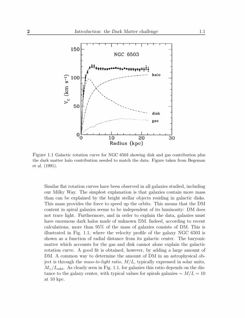
Figure 1.1 Galactic rotation curve for NGC 6503 showing disk and gas contribution plusthe dark matter halo contribution needed to match the data. Figure taken from Begemanet al. (1991).
Similar flat rotation curves have been observed in all galaxies studied, includingour Milky Way. The simplest explanation is that galaxies contain more massthan can be explained by the bright stellar objects residing in galactic disks.This mass provides the force to speed up the orbits. This means that the DMcontent in spiral galaxies seems to be independent of its luminosity: DM doesnot trace light. Furthermore, and in order to explain the data, galaxies musthave enormous dark halos made of unknown DM. Indeed, according to recentcalculations, more than 95% of the mass of galaxies consists of DM. This isillustrated in Fig. 1.1, where the velocity profile of the galaxy NGC 6503 isshown as a function of radial distance from its galactic center. The baryonicmatter which accounts for the gas and disk cannot alone explain the galacticrotation curve. A good fit is obtained, however, by adding a large amount ofDM. A common way to determine the amount of DM in an astrophysical ob-ject is through the mass-to-light ratio, M/L, typically expressed in solar units,M⊙/Lodot. As clearly seen in Fig. 1.1, for galaxies this ratio depends on the dis-tance to the galaxy center, with typical values for spirals galaxies ∼ M/L = 10at 10 kpc.

1.1 Observational evidences for Dark Matter 3
The limitations of rotations curves are that they can only be measured up todistances of some tens of kpc, since the observations are based on the distri-bution of light or neutral hydrogen (21 cm). Therefore, we are only obtaininginformation about the very inner parts of DM haloes, and nothing about thoseplaces where most of the DM is (lensing experiments or satellite dynamicscan skip these limitations, as I will discuss below). Because of that, the totalamount of DM present is difficult to quantify. However, despite the uncer-tainties of the slope in the innermost regions of galaxies, rotation curves ofdisk galaxies provide strong evidence for the existence of a spherical DM halo.Additional evidence for DM at galactic scales comes from mass modeling ofthe most detailed rotation curves available, such as spiral arm features. Othergalaxies also show evidence for DM via strong gravitational lensing (Koopmans& Treu 2003). In addition, X-ray evidence reveals the presence of extendedatmospheres of hot gas that fill the DM halos of isolated ellipticals and whosehydrostatic support provides evidence for DM as well (Fabian & Allen 2003).Lensing measurements also confirm the existence of enormous quantities of DMin galaxies. The Sloan Digital Sky Survey used weak lensing (statistical stud-ies of lensed galaxies) to conclude that galaxies, including the Milky Way, areeven larger and more massive than previously thought, and require even moreDM out to great distances (Adelman-McCarthy et al. 2006). This techniquecan study the DM distribution to much larger distances than could be probedby rotation curves: the DM is seen in galaxies out to 200 kpc from their centers.
There are other observations both on subgalactic and intergalactic scales thatpoint in the same direction, i.e. that a large amount of DM is needed in orderto explain the observed properties. We can cite some of them, as compiled inBertone (2005):
• Weak modulation of strong lensing around individual massive ellipticalgalaxies. This provides evidence for substructure on scales of ∼106 M⊙[Metcalf et al. 2004; Moustakas & Metcalf 2003).
• The so-called Oort discrepancy in the disk of the Milky Way (see e.g.Bahcall et al. 1992). The argument follows an early suggestion of Oort,inferring the existence of unobserved matter from the inconsistency be-tween the amount of stars, or other tracers in the solar neighborhood, andthe gravitational potential implied by their distribution.
• Weak gravitational lensing of distant galaxies by foreground structure (seee.g. Hoekstra et al. 2002).
• The velocity dispersions of dwarf spheroidal galaxies which imply mass-to-light ratios larger than those observed in our “local” neighborhood. While

4 Introduction: the Dark Matter challenge 1.1
the profiles of individual dwarfs show scatter, there is no doubt about theoverall DM content (see Vogt et al. 1995; Mateo 1998; Strigari et al. 2008).
• The velocity dispersions of galaxy satellites which suggest the existenceof DM halos around their host galaxies, similar to our own, extending atgalactocentric radii larger than 200 kpc, i.e. well beyond the optical disc.This applies in particular to the Milky Way, where both dwarf galaxy satel-lites and globular clusters probe the outer DM halo (Zaritsky et al. 1997;Prada et al. 2003).
2. Galaxy Clusters scales: In 1933, F. Zwicky inferred, from measurements ofthe velocity dispersion of galaxies in the Coma cluster, a mass-to-light ratioof around 400 solar masses per solar luminosity (Zwicky 1933). This was thefirst modern hint of the presence of large amounts of DM in the Universe. Atpresent, observations of galactic clusters continue to be of central importance inunderstanding the DM problem. Today, most dynamical estimates (Bahcall &Fan 1998; Kashlinsky 1998, Carlberg et al. 1999) are consistent with a value ofM/L ∼ 200− 300 on cluster scales. Another piece of gravitational evidence forDM in clusters is the existence of huge amounts of hot gas in the intraclustermedium. This can be clearly seen in the top panels of Fig. 1.2 for the ComaCluster. The existence of this gas in the cluster can only be explained by alarge DM component that provides the potential well to hold on to the gas.Similar findings were recently discovered in the famous Bullet cluster (see rightbottom panel in Fig. 1.2).
That individual galaxies and galaxy clusters are completely dominated by DMwith the visible baryonic matter being subdominant is demonstrated with-out doubt also in analyses of strong lensing of background galaxies (Tysonet al. 1998) (see left bottom panel in Fig. 1.2 The gravitational lensing analysisof (Falco et al. 1998), based on the frequency of double images in large sur-veys of quasars, indicates that there is plenty of DM. Also observations of theLyman-α forest (Weinberg et al. 1999), combined with the observed mass func-tion of galaxy clusters, clearly need from a substantial amount of non-baryonicDM. Still on very large scales, analyses of the peculiar velocity “flow” of largeclusters and other structures seem to need a lot of DM for its explanation (Si-gal et al. 1998). It is interesting to note that cluster mass estimates based ongravitational lensing, X-ray emission, the SZ effect and galaxy motions all givesimilar mass estimates within about a factor of two.
3. Cosmological scales: Further evidence for DM comes from measurements oncosmological scales of anisotropies in the CMB (Spergel et al. 2007). Given therelevance of the CMB for the present status of Cosmology, this issue will bediscussed in detail in Section 1.2.2). Also the Sunyayev-Zel’dovich (SZ) effectcan be used to extract the amount on non-baryonic DM, by which the CMB

1.2 The ΛCDM paradigm 5
Figure 1.2 Top panels: Without dark matter, the hot gas in the Coma Cluster wouldevaporate. Optical image in the left; X-ray image from ROSAT satellite in the right (Briel& Henry 1997). Left bottom panel: A good example of strong gravitational lensing isthe Abell 1689 galaxy cluster. Right bottom panel: A collision of galactic clusters (theBullet cluster) shows baryonic matter (pink) as separate from dark matter (blue), whosedistribution is deduced from gravitational lensing (Clowe et al. 2006).
gets spectrally distorted through Compton scattering on hot electrons in galaxyclusters. With present SZ data, it is estimated that ∼25% of the Universe is inthe form of DM (Holder and Carlstrom 1999). In addition, recent predictionsfor the primordial nucleosynthesis exactly match the data as long as atoms areonly 4% of the total constituents of the Universe.
1.2 The ΛCDM paradigm
Nowadays, most of the astrophysical community seems to agree in a standard cos-mological picture of the Universe, the so-called ΛCDM paradigm (from Λ Cold DarkMatter). This general picture did not emerge suddenly; on the contrary, it has to beunderstood as the final result obtained after more than 80 years of continuous de-bate both in the observational and theoretical side. This scenario, based on General
6 Introduction: the Dark Matter challenge 1.2
Relativity, is now capable to explain in general terms the observations, as well as toreconcile them with a congruent theoretical picture of the Universe as a whole andof its evolution.
In the ΛCDM paradigm, the geometry of the Universe is flat (i.e. euclidean) andits energy-density is distributed in ∼4% baryonic matter, ∼23% of still unknown non-baryonic dark matter and roughly 73% of a even more mysterious dark energy. Thisparadigm is settled in the Big Bang scenario, in which the Universe had a beginningin time and is as a system evolving from a highly compressed state existing around1010 years ago. The Big Bang has its roots in the important discoveries of E. Hubblein the 1920s, who realized that all galaxies seem to move away from us. The Big Bangtheory, and more in general, the ΛCDM scenario, has survived to all kinds of tests andobservations until now. Indeed, this huge theoretical and observational effort to refutethe model has derived in a even stronger and extremely sophisticated cosmologicalscenario, that allows us to explain in a satisfactory way the thermal history, relicbackground radiation, abundance of elements, large scale structure (LSS) and manyother properties of the Universe. Nevertheless, our knowledge is still partial, andthere are indeed a lot of open questions that the model will have to face in thecoming years.
1.2.1 A brief mathematical description of the model
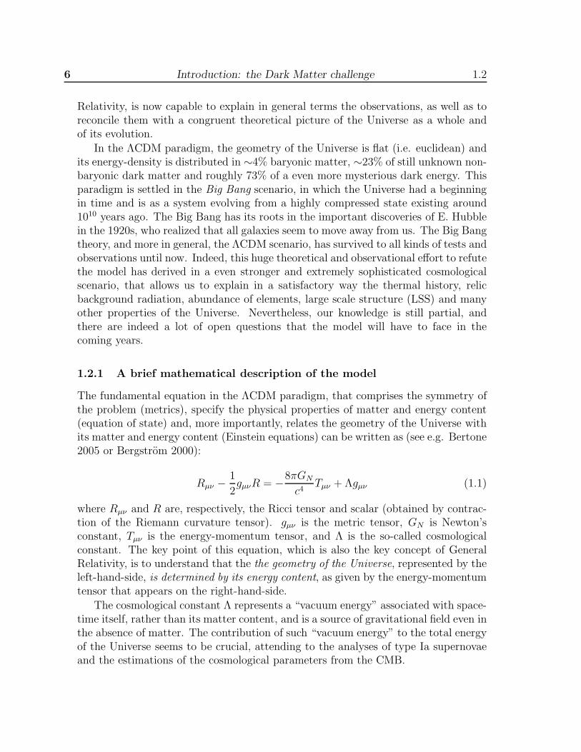
The fundamental equation in the ΛCDM paradigm, that comprises the symmetry ofthe problem (metrics), specify the physical properties of matter and energy content(equation of state) and, more importantly, relates the geometry of the Universe withits matter and energy content (Einstein equations) can be written as (see e.g. Bertone2005 or Bergstrom 2000):
Rµν −1
2gµνR = −8πGN
c4Tµν + Λgµν (1.1)
where Rµν and R are, respectively, the Ricci tensor and scalar (obtained by contrac-tion of the Riemann curvature tensor). gµν is the metric tensor, GN is Newton’sconstant, Tµν is the energy-momentum tensor, and Λ is the so-called cosmologicalconstant. The key point of this equation, which is also the key concept of GeneralRelativity, is to understand that the the geometry of the Universe, represented by theleft-hand-side, is determined by its energy content, as given by the energy-momentumtensor that appears on the right-hand-side.
The cosmological constant Λ represents a “vacuum energy” associated with space-time itself, rather than its matter content, and is a source of gravitational field even inthe absence of matter. The contribution of such “vacuum energy” to the total energyof the Universe seems to be crucial, attending to the analyses of type Ia supernovaeand the estimations of the cosmological parameters from the CMB.

1.2 The ΛCDM paradigm 7
To solve the above equation it is necessary to introduce a symmetry for the prob-lem. Cosmologists typically suppose homogeneity and isotropy for the whole Universe,as confirmed by the most recent observations. This simplifies a lot the mathemati-cal analysis. High isotropy is supported for example by CMB data; homogeneity atscales &100 Mpc seems to be very near reality according to recent galaxy surveyslike SDSS (Tegmark et al. 2004) or 2dF-GRS (Cole et al. 2005). With isotropy andhomogeneity, the line element can be expressed as:
ds2 = −c2dt2 + a(t)2
(
dr2
1 − kr2+ r2dΩ2
)
, (1.2)
where a(t) is the so-called scale factor and the constant k, describing the spatialcurvature, can take the values k = −1, 0, +1 (which means open, flat and closeduniverse respectively). Given this metric, it is possible to solve the Einstein equationsand get the Friedmann equation:
H2 ≡(
a
a
)2
+k
a2=
8πGN
3ρtot +
Λ
3(1.3)
where ρtot is the total average energy density of the universe, and H is the Hubbleparameter. The most recent value achieved for the Hubble parameter at present time,also known as H0 or Hubble constant, is H0 = 72 ± 1 km s−1 Mpc−1 (Hinshaw etal. 2009). In Eq. 1.3, the Universe is flat (k = 0) provided that the energy densityequals the critical density, ρc, i.e.:
ρc ≡3H2
8πGN. (1.4)
The abundance of a substance in the Universe (matter, radiation or vacuum en-ergy) is usually expressed in units of ρc. Let us define the quantity Ωi of a substanceof species i and density ρi as Ωi ≡ ρi
ρc. At the present epoch, we have for the matter,
cosmological constant, radiation and curvature respectively:
Ωm ≡ 8πGNρm
3H20
ΩΛ ≡ Λ
3H20
(1.5)
Ωr ≡8πGNρr
3H20
Ωk ≡ −ka2
0H20
(1.6)
Following with these sort of definitions, it is also useful Ω =∑
i Ωi. Therefore,now we can rewrite the Friedmann equation for the present epoch simply as 1 =Ωm + ΩΛ + Ωr, where the radiation contribution is typically neglected due to its tinyvalue today (∼10−5).
By the other side, the expansion of the Universe means that the scale factor a(t)has been increasing since the earliest times after the Big Bang. This affects the light
8 Introduction: the Dark Matter challenge 1.2
emitted by distant objects. In particular, for an emitted wavelength λemit and anobserved wavelength λobs, the redshift z is given by:
1 + z ≡ λobs
λemit
. (1.7)
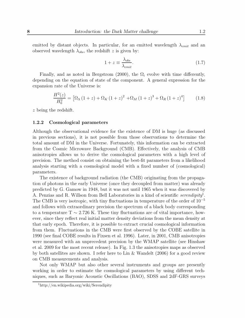
Finally, and as noted in Bergstrom (2000), the Ωi evolve with time differently,depending on the equation of state of the component. A general expression for theexpansion rate of the Universe is:
H2(z)
H20
=[
ΩΛ (1 + z) + ΩK (1 + z)2 +ΩM (1 + z)3 + ΩR (1 + z)4] (1.8)
z being the redshift.
1.2.2 Cosmological parameters
Although the observational evidence for the existence of DM is huge (as discussedin previous sections), it is not possible from those observations to determine thetotal amount of DM in the Universe. Fortunately, this information can be extractedfrom the Cosmic Microwave Background (CMB). Effectively, the analysis of CMBanisotropies allows us to derive the cosmological parameters with a high level ofprecision. The method consist on obtaining the best-fit parameters from a likelihoodanalysis starting with a cosmological model with a fixed number of (cosmological)parameters.
The existence of background radiation (the CMB) originating from the propaga-tion of photons in the early Universe (once they decoupled from matter) was alreadypredicted by G. Gamow in 1948, but it was not until 1965 when it was discovered byA. Penzias and R. Willson from Bell Laboratories in a kind of scientific serendipity1.The CMB is very isotropic, with tiny fluctuations in temperature of the order of 10−5
and follows with extraordinary precision the spectrum of a black body correspondingto a temperature T ∼ 2.726 K. These tiny fluctuations are of vital importance, how-ever, since they reflect real initial matter density deviations from the mean density atthat early epoch. Therefore, it is possible to extract crucial cosmological informationfrom them. Fluctuations in the CMB were first observed by the COBE satellite in1990 (see final COBE results in Fixsen et al. 1996). Later, in 2001, CMB anisotropieswere measured with an unprecedent precision by the WMAP satellite (see Hinshawet al. 2009 for the most recent release). In Fig. 1.3 the anisotropies maps as observedby both satellites are shown. I refer here to Lin & Wandelt (2006) for a good reviewon CMB measurements and analysis.
Not only WMAP but also other several instruments and groups are presentlyworking in order to estimate the cosmological parameters by using different tech-niques, such as Baryonic Acoustic Oscillations (BAO), SDSS and 2dF-GRS surveys
1http://en.wikipedia.org/wiki/Serendipity

1.2 The ΛCDM paradigm 9
Figure 1.3 CMB anisotropy maps (i.e. maps of temperature fluctuations), as obtained bythe COBE satellite (top) and by the more recent WMAP (bottom). Credit: NASA.
data, detailed observations of distant Supernova type Ia, etc. Indeed, observationscarried out by the Supernova Cosmology Project and the High-z Supernova SearchTeam in the last 1990s represented the first solid evidence of the (now almost un-doubted and well established and accepted) fact that the Universe is accelerating(Riess et al. 1998; Perlmutter et al. 1999), which was interpreted as due to a cosmo-logical constant Λ or, more generically, to a “dark energy” dominant component inthe Universe. Figure 1.4 (actually a table) summarizes the cosmological parametersas deduced for the WMAP team after the analysis of 5-years CMB data obtainedwith this satellite (Hinshaw et al. 2009). Also shown are the cosmological parametersdeduced when crossing WMAP results with those obtained from BAO and super-novae. This Table represents the most refined ΛCDM cosmological model available atpresent, i.e. the 21st century state-of-the-art Cosmology. Nevertheless, it is expectedthat the Planck satellite, which was successfully launched last May, 14th 2009 andwhich represents the natural WMAP successor, improves these records even more2.
2http://sci.esa.int/science-e/www/area/index.cfm?fareaid=17

10 Introduction: the Dark Matter challenge 1.2
–
Description Symbol WMAP-only WMAP+BAO+SN
Parameters for Standard ΛCDM Model a
Age of universe t0 13.69 ± 0.13 Gyr 13.73 ± 0.12 Gyr
Hubble constant H0 71.9+2.6−2.7 km/s/Mpc 70.1 ± 1.3 km/s/Mpc
Baryon density Ωb 0.0441 ± 0.0030 0.0462 ± 0.0015
Physical baryon density Ωbh2 0.02273 ± 0.00062 0.02265 ± 0.00059
Dark matter density Ωc 0.214 ± 0.027 0.233 ± 0.013
Physical dark matter density Ωch2 0.1099 ± 0.0062 0.1143 ± 0.0034
Dark energy density ΩΛ 0.742 ± 0.030 0.721 ± 0.015
Curvature fluctuation amplitude, k0 = 0.002 Mpc−1 b ∆2R
(2.41 ± 0.11) × 10−9 (2.457+0.092−0.093) × 10−9
Fluctuation amplitude at 8h−1 Mpc σ8 0.796 ± 0.036 0.817 ± 0.026
l(l + 1)CTT220/2π C220 5756 ± 42 µK2 5748 ± 41 µK2
Scalar spectral index ns 0.963+0.014−0.015 0.960+0.014
−0.013
Redshift of matter-radiation equality zeq 3176+151−150 3280+88
−89
Angular diameter distance to matter-radiation eq.c dA(zeq) 14279+186−189 Mpc 14172+141
−139 Mpc
Redshift of decoupling z∗ 1090.51 ± 0.95 1091.00+0.72−0.73
Age at decoupling t∗ 380081+5843−5841 yr 375938+3148
−3115 yr
Angular diameter distance to decoupling c,d dA(z∗) 14115+188−191 Mpc 14006+142
−141 Mpc
Sound horizon at decoupling d rs(z∗) 146.8 ± 1.8 Mpc 145.6 ± 1.2 Mpc
Acoustic scale at decoupling d lA(z∗) 302.08+0.83−0.84 302.11+0.84
−0.82
Reionization optical depth τ 0.087 ± 0.017 0.084 ± 0.016
Redshift of reionization zreion 11.0 ± 1.4 10.8 ± 1.4
Age at reionization treion 427+88−65 Myr 432+90
−67 Myr
Parameters for Extended Models e
Total density f Ωtot 1.099+0.100−0.085 1.0052 ± 0.0064
Equation of state g w −1.06+0.41−0.42 −0.972+0.061
−0.060
Tensor to scalar ratio, k0 = 0.002 Mpc−1 b,h r < 0.43 (95% CL) < 0.20 (95% CL)
Running of spectral index, k0 = 0.002 Mpc−1 b,i dns/d ln k −0.037 ± 0.028 −0.032+0.021−0.020
Neutrino density j Ωνh2 < 0.014 (95% CL) < 0.0065 (95% CL)
Neutrino mass jP
mν < 1.3 eV (95% CL) < 0.61 eV (95% CL)
Number of light neutrino families k Neff > 2.3 (95% CL) 4.4 ± 1.5
Figure 1.4 Cosmological parameters obtained after 5 years of WMAP observations (thirdcolumn) and after crossing the 5-years WMAP results with other techniques (BarionicAcoustic Oscillations and Supernovae; fourth column), as presented in Hinshaw et al. (2009).See this same work for more details.
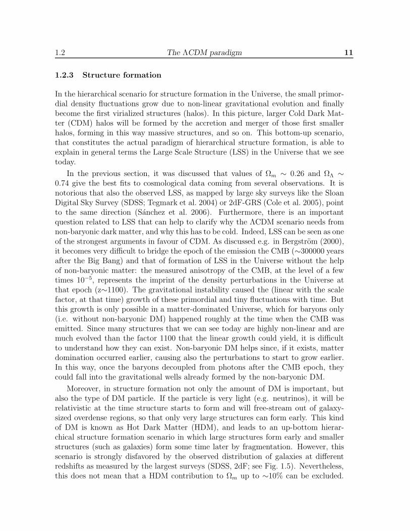
1.2 The ΛCDM paradigm 11
1.2.3 Structure formation
In the hierarchical scenario for structure formation in the Universe, the small primor-dial density fluctuations grow due to non-linear gravitational evolution and finallybecome the first virialized structures (halos). In this picture, larger Cold Dark Mat-ter (CDM) halos will be formed by the accretion and merger of those first smallerhalos, forming in this way massive structures, and so on. This bottom-up scenario,that constitutes the actual paradigm of hierarchical structure formation, is able toexplain in general terms the Large Scale Structure (LSS) in the Universe that we seetoday.
In the previous section, it was discussed that values of Ωm ∼ 0.26 and ΩΛ ∼0.74 give the best fits to cosmological data coming from several observations. It isnotorious that also the observed LSS, as mapped by large sky surveys like the SloanDigital Sky Survey (SDSS; Tegmark et al. 2004) or 2dF-GRS (Cole et al. 2005), pointto the same direction (Sanchez et al. 2006). Furthermore, there is an importantquestion related to LSS that can help to clarify why the ΛCDM scenario needs fromnon-baryonic dark matter, and why this has to be cold. Indeed, LSS can be seen as oneof the strongest arguments in favour of CDM. As discussed e.g. in Bergstrom (2000),it becomes very difficult to bridge the epoch of the emission the CMB (∼300000 yearsafter the Big Bang) and that of formation of LSS in the Universe without the helpof non-baryonic matter: the measured anisotropy of the CMB, at the level of a fewtimes 10−5, represents the imprint of the density perturbations in the Universe atthat epoch (z∼1100). The gravitational instability caused the (linear with the scalefactor, at that time) growth of these primordial and tiny fluctuations with time. Butthis growth is only possible in a matter-dominated Universe, which for baryons only(i.e. without non-baryonic DM) happened roughly at the time when the CMB wasemitted. Since many structures that we can see today are highly non-linear and aremuch evolved than the factor 1100 that the linear growth could yield, it is difficultto understand how they can exist. Non-baryonic DM helps since, if it exists, matterdomination occurred earlier, causing also the perturbations to start to grow earlier.In this way, once the baryons decoupled from photons after the CMB epoch, theycould fall into the gravitational wells already formed by the non-baryonic DM.
Moreover, in structure formation not only the amount of DM is important, butalso the type of DM particle. If the particle is very light (e.g. neutrinos), it will berelativistic at the time structure starts to form and will free-stream out of galaxy-sized overdense regions, so that only very large structures can form early. This kindof DM is known as Hot Dark Matter (HDM), and leads to an up-bottom hierar-chical structure formation scenario in which large structures form early and smallerstructures (such as galaxies) form some time later by fragmentation. However, thisscenario is strongly disfavored by the observed distribution of galaxies at differentredshifts as measured by the largest surveys (SDSS, 2dF; see Fig. 1.5). Nevertheless,this does not mean that a HDM contribution to Ωm up to ∼10% can be excluded.
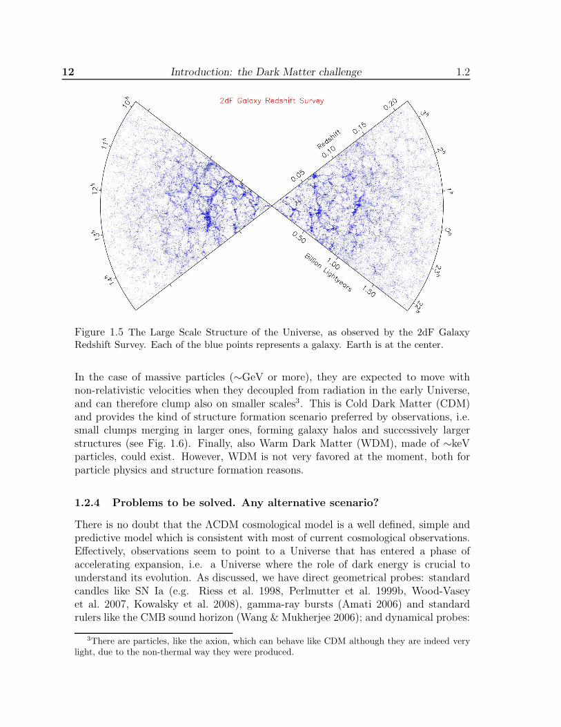
12 Introduction: the Dark Matter challenge 1.2
Figure 1.5 The Large Scale Structure of the Universe, as observed by the 2dF GalaxyRedshift Survey. Each of the blue points represents a galaxy. Earth is at the center.
In the case of massive particles (∼GeV or more), they are expected to move withnon-relativistic velocities when they decoupled from radiation in the early Universe,and can therefore clump also on smaller scales3. This is Cold Dark Matter (CDM)and provides the kind of structure formation scenario preferred by observations, i.e.small clumps merging in larger ones, forming galaxy halos and successively largerstructures (see Fig. 1.6). Finally, also Warm Dark Matter (WDM), made of ∼keVparticles, could exist. However, WDM is not very favored at the moment, both forparticle physics and structure formation reasons.
1.2.4 Problems to be solved. Any alternative scenario?
There is no doubt that the ΛCDM cosmological model is a well defined, simple andpredictive model which is consistent with most of current cosmological observations.Effectively, observations seem to point to a Universe that has entered a phase ofaccelerating expansion, i.e. a Universe where the role of dark energy is crucial tounderstand its evolution. As discussed, we have direct geometrical probes: standardcandles like SN Ia (e.g. Riess et al. 1998, Perlmutter et al. 1999b, Wood-Vaseyet al. 2007, Kowalsky et al. 2008), gamma-ray bursts (Amati 2006) and standardrulers like the CMB sound horizon (Wang & Mukherjee 2006); and dynamical probes:
3There are particles, like the axion, which can behave like CDM although they are indeed verylight, due to the non-thermal way they were produced.
1.2 The ΛCDM paradigm 13
Figure 1.6 CDM is needed in order to obtain the kind of bottom-up hierarchical structureformation favored by present observations (see Fig. 1.5), as well as to explain the abundancesof substructure in the Universe. From left to right: LSS with CDM, WDM and HDM, seetext for details. Credit: B. Moore.
growth rate of cosmological perturbations (Polarski & Gannouji 2008) probed by theredshift distortion factor or by weak lensing (Munshi et al. 2008). However, there aresome specific observations which differ from the predictions of the ΛCDM scenario(with those cosmological parameters given by 5-years WMAP data) at a level of 2σor higher, such as (Perivolaropoulos 2008):
• Large Scale Velocity Flows: ΛCDM predicts significantly smaller amplitudeand scale of flows than what observations indicate (e.g. Watkins et al. 2008,Kashlinsky et al. 2008).
• Brightness of Type Ia Supernovae (SNIa) at High Redshift: ΛCDM predictsfainter SNIa at high z (Perivolaropoulos & Shafieloo 2008).
• Emptiness of Voids: ΛCDM predicts more dwarf or irregular galaxies in voidsthan observed (e.g. Tikhonov & Klypin).
• Profiles of Cluster Haloes: ΛCDM predicts shallow low concentration and den-sity profiles in contrast to observations which indicate denser high concentrationcluster haloes (Broadhurst et al. 2008).
14 Introduction: the Dark Matter challenge 1.2
• Profiles of Galaxy Haloes: ΛCDM predicts halo mass profiles with cuspy coresand low outer density while lensing and dynamical observations indicate a cen-tral core of constant density and a flattish high dark mass density outer profile(de Blok 2005; Gentile et al. 2005).
• “Missing satellites problem”: N-body ΛCDM cosmological simulations seem togive much more substructure of DM within clusters and galactic halos than whatis observed (e.g. Klypin et al. 1999). It is not clear, however, how serious theseproblems are in view of the large uncertainties and different results obtainedby different groups working in the field. Moreover, the recent discoveries ofultrafaint dwarfs in the Milky Way halo may alleviate this problem considerably(see Kravtsov 2009 for a recent review on this issue).
• Sizable Population of Disk Galaxies: ΛCDM predicts a smaller fraction of diskgalaxies due to recent mergers expected to disrupt cold rotationally supporteddisks (Bullock et al. 2008).
Not all the above mentioned problems have probably similar importance. Perhapsthe most difficult ones are those related with the rotation in the inner parts of spiralgalaxies, where the theory predicts too much DM inside the central ∼ 1 kpc (Moore1994, Flores & Primack 1994, de Blok et al. 2001). Some solutions have beenproposed to this problem (see e.g. Valenzuela et al. 2007), but still the descriptionof what happens at small scales is the strongest challenge the ΛCDM cosmologicalmodel has encountered.
There are also some weak points from the theoretical point of view concerningthe ΛCDM model (e.g. Copeland et al. 2006):
• The Fine Tuning Problem: What is the physical mechanism that sets the valueof Λ to its observed value which is 120 orders of magnitude smaller than thephysically anticipated value, i.e. the natural energy scale of Quantum Gravity?
• The Coincidence Problem: Why is the energy density corresponding to thecosmological constant just starting to dominate the Universe at the presentcosmological time?
Even though some of the above given puzzles may be resolved by more completeobservations or with conventional astrophysics still inside the standard model, morefundamental modifications of the ΛCDM model should not be excluded at present.A significant effort has been made for several people in order to build alternativecosmological models. That is the case of Modified Newtonian Dynamics (MOND),initially proposed by Milgrom (1983) to explain the rotation of galaxies withoutDM. According to MOND, the rotation curves in the outer regions of galaxies donot decline because the force of gravity is significantly stronger than for Newtoniangravity.
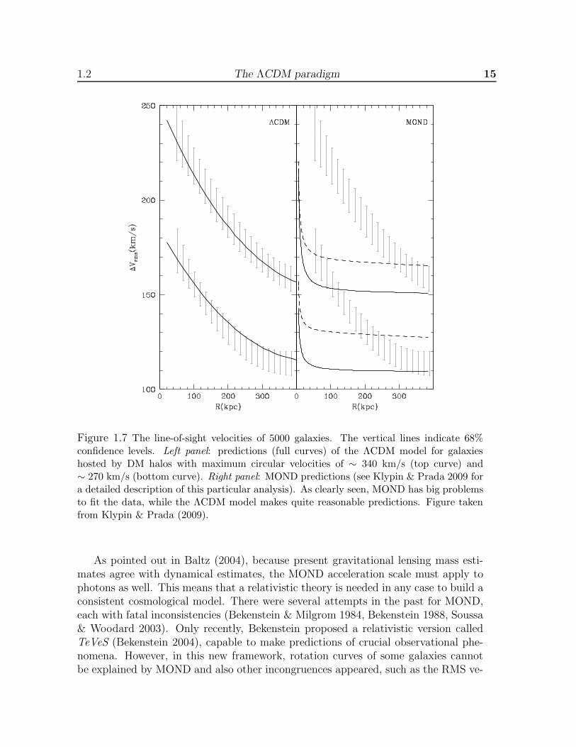
1.2 The ΛCDM paradigm 15
Figure 1.7 The line-of-sight velocities of 5000 galaxies. The vertical lines indicate 68%confidence levels. Left panel: predictions (full curves) of the ΛCDM model for galaxieshosted by DM halos with maximum circular velocities of ∼ 340 km/s (top curve) and∼ 270 km/s (bottom curve). Right panel: MOND predictions (see Klypin & Prada 2009 fora detailed description of this particular analysis). As clearly seen, MOND has big problemsto fit the data, while the ΛCDM model makes quite reasonable predictions. Figure takenfrom Klypin & Prada (2009).
As pointed out in Baltz (2004), because present gravitational lensing mass esti-mates agree with dynamical estimates, the MOND acceleration scale must apply tophotons as well. This means that a relativistic theory is needed in any case to build aconsistent cosmological model. There were several attempts in the past for MOND,each with fatal inconsistencies (Bekenstein & Milgrom 1984, Bekenstein 1988, Soussa& Woodard 2003). Only recently, Bekenstein proposed a relativistic version calledTeVeS (Bekenstein 2004), capable to make predictions of crucial observational phe-nomena. However, in this new framework, rotation curves of some galaxies cannotbe explained by MOND and also other incongruences appeared, such as the RMS ve-

16 Introduction: the Dark Matter challenge 1.3
locities of stars in some dwarf spheroidal galaxies (Lokas et al. 2006). Still, the mostimportant problems for MOND are those related to clusters of galaxies. Dynamicsof galaxies in clusters cannot be explained by MOND and requires introduction ofDM, possibly in the form of a massive (∼ 2eV) neutrino (Sanders et al. 2002). InFig. 1.7 a comparison between those predictions coming from the ΛCDM model andthose coming from MOND for a specific astrophysical case is shown.
Despite the problems of MOND (which is only the most famous among all thepossible alternative proposed scenarios to ΛCDM), the key point of this subsection,however, remains completely valid: there is no simple cosmological model which doesnot have problem with at least some sets of data. Therefore, it is worth keeping severalpossibilities open, while awaiting data of even higher precision that helps to refineeven more the ΛCDM model or to build new and testable theoretical frameworks tobe explored.
1.3 Dark Matter and N-body cosmological simulations
Although we are confident to have reached a general picture of large scale structure(LSS), our understanding is still far from to be completed. The description of theevolution of structures from primordial density fluctuations, is complicated by theaction of many physical processes like gas dynamics, radiative cooling, photoioniza-tion, recombination and radiative transfer. The most widely adopted approach to theproblem of LSS formation involves the use of N-body cosmological simulations (seeBagla 2005 for a review). The first simulation was performed by Holmberg (1941) oninteracting galaxies. He used an analog optical computer. At present, high resolutionsimulations make full use of the tremendous computational power available.
In Cosmology, the evolution of structure is often approximated with non-lineargravitational clustering from specified initial conditions of DM particles and can berefined by introducing the effects of gas dynamics, chemistry, radiative transfer andother astrophysical processes. In principle, N-body simulations are simple, since theyjust involve integrating the 6N ordinary differential equations defining the particlemotions in Newtonian gravity. In practice, the problem is the huge number N ofparticles (the highest resolution simulations at present include many millions, seeFig. 1.8). Since the number of interactions needing to be computed is proportional toN2, ordinary methods of integrating numerical differential equations are inadequate.Therefore, a number of refinements are commonly used. By the other side, manysimulations simulate only CDM (∼5/6 of the total matter content of the Universe),and therefore include only the gravitational force. Incorporating baryons in the sim-ulations dramatically increases their complexity. A large effort is being carried out atpresent by several groups in order to successfully implement them in the simulations,since they are expected to be crucial in the understanding of astrophysical processessuch as galaxy formation.
The reliability of an N-body simulation is measured by its mass and length resolu-
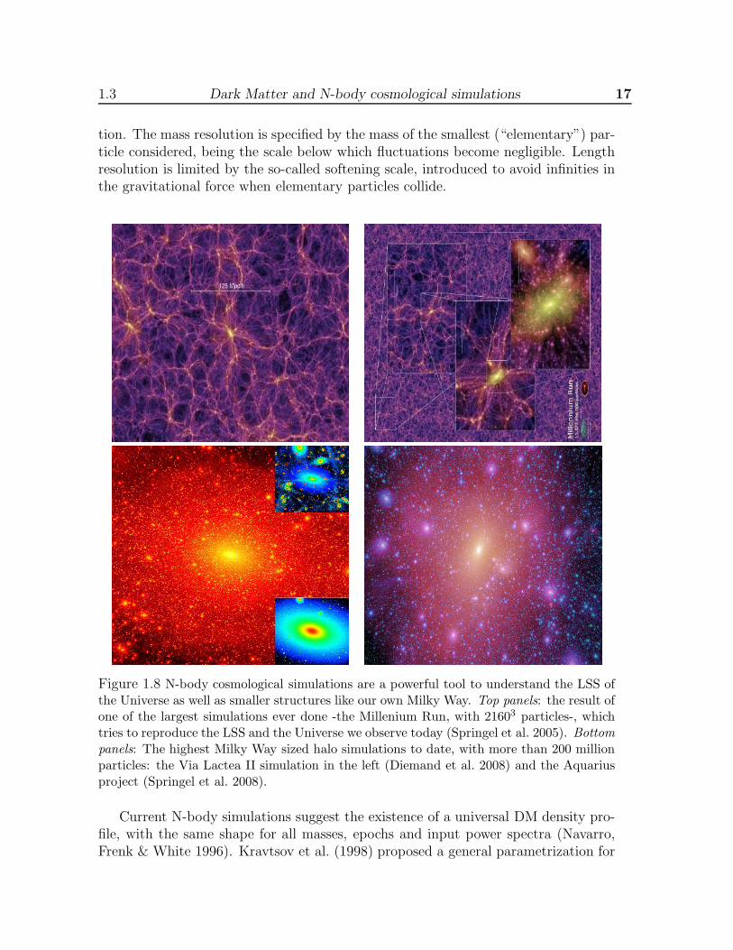
1.3 Dark Matter and N-body cosmological simulations 17
tion. The mass resolution is specified by the mass of the smallest (“elementary”) par-ticle considered, being the scale below which fluctuations become negligible. Lengthresolution is limited by the so-called softening scale, introduced to avoid infinities inthe gravitational force when elementary particles collide.
Figure 1.8 N-body cosmological simulations are a powerful tool to understand the LSS ofthe Universe as well as smaller structures like our own Milky Way. Top panels: the result ofone of the largest simulations ever done -the Millenium Run, with 21603 particles-, whichtries to reproduce the LSS and the Universe we observe today (Springel et al. 2005). Bottom
panels: The highest Milky Way sized halo simulations to date, with more than 200 millionparticles: the Via Lactea II simulation in the left (Diemand et al. 2008) and the Aquariusproject (Springel et al. 2008).
Current N-body simulations suggest the existence of a universal DM density pro-file, with the same shape for all masses, epochs and input power spectra (Navarro,Frenk & White 1996). Kravtsov et al. (1998) proposed a general parametrization for
18 Introduction: the Dark Matter challenge 1.3
the DM halo density in order to agglutinate most of the fitting formulae that can befound in the literature:
ρ(r) = ρs/[(r/rs)γ (1 + (r/rs)
α)(β−γ)/α], (1.9)
where ρs and rs represent a characteristic density and a scale radius respectively.Effectively, these density profiles are well motivated by high-resolution N-body cos-mological simulations. The Navarro-Frenk-White (Navarro, Frenk & White 1997;hereafter NFW), with (α,β,γ) = (1,3,1), and Moore profiles (Moore et al. 1998),with (α,β,γ) = (1.5,3,1.5), are some examples of the most widely DM density profilesused in the literature so far (see Fig. 1.9). As it can be seen from these values, variousgroups have ended up with different results for the spectral shape in the innermostregions of galaxies and galaxy clusters, which are by far the most conflictive regionsto be simulated, given the short dynamical time-scales and strong gravitational forces(which also means a more expensive computational cost). For this Thesis, the DMdensity profile inner slope will become crucial in the estimations of the DM annihi-lation flux, as we will see later in more detail. Also related to this issue, the effectsof the adiabatic baryonic compression of the DM near the center of haloes, typicallydiscarded in N-body simulations, may enhance the DM density considerably (up toone order of magnitude according to Prada et al. 2004), as well as the possible ef-fect of central black holes (see Gnedin & Primack 2004 or Diemand et al. 2005 fordiscussion on this particular issue).
N-body cosmological simulations based on the ΛCDM paradigm are in good agree-ment with a wide range of observations, such as the abundance of clusters at z ≤ 1 andthe galaxy-galaxy correlation functions (see e.g. Primack 2001 for a review of CDM).However, as pointed out e.g. in Taoso et al. (2008), there are important discrepan-cies, some of them already discussed in subsection 1.2.4. For example, the numberof satellite halos in Milky Way-sized galaxies, as predicted by simulations, exceedsthe number of observed dwarf galaxies (Moore et al. 1999, Klypin et al. 1999). Therotation curves of low surface brightness (LSB) disk galaxies point to DM distribu-tions with constant density cores rather than the cuspy profiles preferred by N-bodysimulations (Flores & Primack 1994; McGaugh & de Blok 1998). As for the angularmomentum of DM halos, in simulations gas cools at early time into small mass halos,leading to massive low-angular momentum cores in conflict with the observed expo-nential disks (Bullock et al. 2001). However, astrophysical processes such as majormergers and astrophysical feedback might help to solve these problems (Vitvitskaet al. 2002). The low efficiency of gas cooling and star formation may decrease thenumber of satellites in Milky Way-sized galaxies (e.g. Moore et al. 2006) as well astidal stripping (e.g. Kravtsov et al. 2004). Furthermore, new ultra-faint dwarf galax-ies recently detected with SDSS data seems to importantly alleviate the discrepancybetween CDM predictions and observations, as also discussed in previous sections(Simon & Geha 2007). The measurements of the LSB galaxies rotation curves maysuffer of observational biases, for example due to the fact that DM halos are triaxials

1.4 What is Dark Matter made of? 19
Figure 1.9 Top: Logarithmic slope of the density profile of the Via Lactea simulation asa function of radius. The thin line shows the slope of the best-fit NFW profile. Bottom:Residuals in percent between the density profile and the best-fit NFW profile. Figure takenfrom Diemand et al. (2007).
rather than spherically symmetric (Hayashi et al. 2007). Moreover, small deviationsof the primordial power spectrum from scale invariance, the presence of neutrinos(Hofmann et al. 2001) or astrophysical processes (e.g. Weinberg & Katz 2002) cansensibly affect the halo profiles.
1.4 What is Dark Matter made of?
We have already discussed in previous sections that there is a lot of observationalevidence of the existence of Dark Matter. The natural question now is which kindof particles can account for the huge fraction of the total content of the Universepredicted to be in the form of DM. Up to now, a plethora of DM candidates havebeen proposed. For example, MACHOs, or Massive Compact Halo Objects, which
20 Introduction: the Dark Matter challenge 1.4
are still baryonic DM in the form of faint stars or stellar remnants. However, weknow that they do not exist in sufficient quantity to completely resolve the DMchallenge. It seems necessary to make use of physics beyond the Standard Modelof Particle Physics, where good non-baryonic DM candidates arise that fulfill all thecosmological requirements. The most popular are probably the neutralinos and theaxions, both of them proposed for other reasons in extensions of the Standard Modelof particle physics. Ordinary massive neutrinos are too light to be cosmologicallysignificant, though sterile neutrinos remain a possibility. Other candidates includeprimordial black holes, non-thermal WIMPzillas, and Kaluza-Klein particles. In thissection I will briefly review only those candidates with a larger acceptance in thecommunity at present. For a detailed picture, see e.g. Bergstrom (2000), Bertone(2005) or Steffen (2009).
1.4.1 Barionic Dark Matter
It is possible to estimate the baryon density of the Universe from the fraction ofobserved light elements (H, D and He). The found value, however, Ωbaryons ∼ 0.02, istoo low to account for the total DM content needed to explain cosmological data, likethe CMB (which gives a total matter content Ωm ∼0.27), and to explain the observedLSS. Nevertheless, it seems also clear that even the minimum value of Ωbaryons allowedby Big Bang nucleosynthesis (BBN) (Ωbaryons ∼ 0.044) is higher than the contributionfrom luminous baryons. This means that there exists also a DM problem for baryons,i.e. that a high fraction of them will be hidden.
Effectively, it is possible to think about ordinary matter difficult to be observedwith the present technology and current telescopes. For example, apart from therelatively large amounts of hot X-ray emitting gas in clusters, the main baryoniccomponent of the Universe may be diffusively distributed gas in-between galaxiesand clusters difficult to be detected. In addition, it cannot be excluded that a largeamount of baryonic mass may be hidden in galactic halos in the form of sub-solarmass objects, known as MACHOs (from MAssive Compact Halo Objects), thatinclude faint stars, planetary objects (brown dwarfs and Jupiter-like planets), andstellar remnants (white dwarfs, neutron stars, and black holes). In order to detectthem, astrophysicists have used the microlensing technique very specially. The idea isto monitor 1 to 10 million stars in a satellite galaxy, e.g. the Large Magellanic Cloud(LMC) or Small Magellanic Cloud (SMC). The intensity of one of these backgroundstars will rise in a typical, time-symmetric and achromatic fashion during a few days,weeks, or months (depending on the mass and transverse velocity of the interveningobject) if an object such as a non-luminous star passes the line-of-sight to the star(Paczynski 1986) and if such stars make up a sizeable fraction of the Galactic halo.Microlensing experiments, like MACHO (Alcock et al. 2000) and EROS (Ansari etal. 2004), as well as a combination of other observational (HST) and theoreticalresults (Graff & Freese 1996) have shown that MACHOs less massive than 0.1 M⊙
1.4 What is Dark Matter made of? 21
make an insignificant contribution to the energy density of the Galaxy. Alcock etal. (2000) and Freese et al. (2000) claim that roughly 20% halo fraction could bemade at most of ∼0.5 M⊙ objects which might be made of stellar remnants suchas white dwarfs, although this fraction could be probably even smaller according toother works (Zaritsky et al. 1999; Salati et al. 1999). Therefore, the conclusion isthat such experiments evidence that most of the DM in the Galaxy is not in theform of baryons, which is consistent with what it is inferred from CMB-combinedcosmological measurements: most of the DM in the Universe should be non-baryonicmatter.
Finally, and even though there is not much room at present for a major componentof DM in the Universe being of baryonic form, one cannot entirely rule out some exoticbut still baryonic scenarios. However, since many of these invoke “conventional”matter, such as difficult to detect (and exclude) cold molecular clouds or very lowmass stars with an extremely fine-tuned mass function, a major yet unsolved problemfor these models is to circumvent the BBN bound. A form of baryonic DM which couldavoid the BBN bound, for example, is primordial black holes (Ivanov et al. 1994).
1.4.2 Non-baryonic Dark Matter particle candidates
A good DM particle candidate should fulfill a series of important properties (Baltz2004; Taoso et al. 2008) in order to provide a convincing explanation to all theobserved phenomenology:
1. It should be weakly interacting to ordinary matter and electrically neutral, i.e.with neither electromagnetic nor strong interactions.
2. It should be long-lived enough for having been present since the early Universe,when they were created.
3. It has to be cold (see Section 1.2.3 to remember the reasons).
4. It must be massive enough to account for the measured Ωm.
5. It must be consistent with observations (BBN, relic density, stellar evolution,LSS...) and present constraints (direct and indirect detections; see Section 1.5).
These particles are known as Weakly Interacting Massive Particles or, simply,WIMPs.
As also discussed in Baltz (2004), the mass range of the proposed non-baryonicDM candidates covers at least ∼90 orders of magnitude in mass (from e.g. “fuzzy”CDM to WIMPzillas); unfortunately astrophysical observations do not help in con-straining this huge mass range. However, the energy scale ∼100 GeV is of specialinteresting for the DM problem, as we will describe in next sections. In the following,
22 Introduction: the Dark Matter challenge 1.4
I will briefly present some of the preferred DM candidates at present. Again, I referto Bergstrom (2000), Bertone (2005), Buckley et al. (2008b), Steffen (2009) for de-tailed reviews on each of the candidates presented below as well as on other plausiblescenarios.
• Neutrinos: Until very recently, neutrinos were considered excellent DM candi-dates for their “undisputed virtue of being known to exist” (Bergstrom 2000).However, neutrinos are simply not abundant enough to be the dominant DMcomponent: from the analysis of CMB anisotropies, combined with LSS data,we know that Ωνh
2 < 0.0065 (95% confidence limit; see Table 1.4). Further-more, they are hot (HDM), which as discussed in subsection 1.2.3 is disfavoredby current observations. Effectively, being relativistic collisionless particles,neutrinos erase fluctuations below a scale of ∼ 40 Mpc (mν/30 eV) (Bond etal. 1980), which would imply a top-down hierarchical scenario for the formationof structures in the Universe, contrary to present trends.
Also sterile neutrinos have been proposed as CDM; they are similar to standardneutrinos, but without Standard Model weak interactions apart from mixingand can be much heavier. Proposed as DM candidates by Dodelson & Widrow(1993), stringent cosmological and astrophysical constraints on sterile neutrinoscome from the analysis of their cosmological abundance and the study of theirdecay products (Abazajian et al. 2001).
• Axions: the existence of axions requires physics beyond the Standard Modelof particle physics, since they were introduced in an attempt to solve the prob-lem of CP violation. Laboratory searches, stellar cooling and the dynamics ofsupernova 1987A constrain axions to be very light (. 0.01 eV). Because of ax-ions couple so weakly to the rest of matter, they were not produced in thermalequilibrium in the early Universe; therefore, despite their light masses, they canbehave as CDM. Their relic abundance matches the DM cosmological densityfor masses around 10 µeV (although this value is quite uncertain due to theuncertainties in the production mechanisms).
• SUSY candidates: as discussed above, and despite the fact that neutrinosare thought to be massive, they are essentially ruled out as DM candidates.Consequently, the Standard Model does not provide a viable DM candidate.Supersymmetry (SUSY) is capable to provide good DM candidates with all theneeded characteristics enumerated above. Before presenting the SUSY candi-dates, a brief introduction to SUSY seems to be not only convenient but alsonecessary. Further details can be found in a huge number of SUSY reviews (e.g.Wess & Bagger 1992; Jungman et al. 1996; Binetruy et al. 2001).
In particle physics, a solution to the so-called hierarchy problem (why the ex-pected mass of the Higgs particle is so low) requires new physics. An example is
1.4 What is Dark Matter made of? 23
provided by SUSY, a symmetry in nature between fermions and bosons, wherethe supersymmetric partners of standard model particles lead to cancellationsin the radiative corrections to the Higgs mass. SUSY seems to be a necessaryingredient in superstring theory, which unites all the fundamental forces of na-ture, including gravity. SUSY is designed to keep particle masses at the rightvalue. As a consequence, each particle has a partner: photino for the photon,squark for quark, selectron for the electron, and so on. The hierarchy problemin particle physics motivates the existence of new particle degrees of freedomin the mass range of 100 GeV to TeV scale. It is a remarkable coincidencethat if DM is composed of a WIMP with an approximate mass of this order,one could naturally produce the required cosmological density through thermaldecoupling of the DM component (this is the so-called WIMP miracle). Note,however, that supersymmetric DM should be seen just as one particular real-ization of a generic WIMP. Here weakly interacting, electrically neutral massive(GeV to TeV range) particles are assumed to carry a conserved quantum number(R-parity in the case of supersymmetry) which suppresses or forbids the decayinto lighter particles. Such particles should have been copiously produced inthe early universe through their weak interactions with other forms of matterand radiation. As the universe expanded and cooled, the number density ofthe WIMPs successively became too low for the annihilation processes to keepup with the Hubble expansion rate. A relic population of WIMPs should thusexist, and it is very suggestive that the canonical weak interaction strength is,according to detailed calculations, just right to make the relic density fall in therequired range to contribute substantially to the total content of energy-densityof the Universe.
The most preferred DM candidates that arises in the context of SUSY are:
Neutralinos: probably the best WIMP candidate, and the preferred and mostwidely studied as well. In SUSY, if one postulates a conserved quantityarising from some new symmetry (R-parity), the lightest supersymmetricparticle (LSP) is stable and would provide a natural candidate for DM. Infact, as pointed out e.g. in Buckley et al. (2008b), R-parity conservation isintroduced into SUSY not to solve the DM problem, but rather to ensurethe stability of the proton. In many regions of supersymmetric parameterspace, the LSP is the neutralino, a Majorana particle (its own antiparticle)that is the lightest supersymmetric partner to the electroweak and Higgsbosons.
The attractiveness of this candidate, besides its particle physics conve-nience, is that it fulfill all the WIMP requirements with excellent marks.Furthermore, it has gauge couplings and a mass which for a large rangeof parameters in the supersymmetric sector imply a relic density in the
24 Introduction: the Dark Matter challenge 1.5
required range to explain the observed Ωm ∼ 0.3.
Axinos: if the axions proposed to solve the strong CP problem exist andin addition SUSY is valid, the axion will naturally have as a partner theaxino. Their mass ranges between the eV and the GeV scale, and theycan be efficiently produced through thermal and non-thermal processes inthe early Universe under the form of cold, warm or even hot DM (see e.g.Choi & Roszkowski 2006; Covi et al. 2004). In particular, axinos CDM isachieved for masses ≥ 100 keV.
Gravitinos: they are the superpartner of the graviton. It was the first SUSYparticle considered for the DM problem (Pagels & Primack 1982). In mod-els where the gravitino is the LSP, it is often quite light (keV), and wouldthus be warm (WDM). In Cosmology, the overproduction of gravitinos canbe problematic, though the difficulties can be circumvented (Kawasaky etal. 1995). Gravitinos at the weak scale, whose relic density would be ob-tained through the decays of the next lightest superpartner, are also aninteresting possibility (Feng et al. 2003).
• Kaluza-Klein particles: if our four-dimensional space-time is embedded ina higher dimensional space, accessible only at very small length or very highenergy scales, excitations of Standard Model states along the orthogonal dimen-sions (called Kaluza-Klein excitations) may be viable DM candidates as welland act therefore as WIMPs (e.g. Servant & Tait 2003). Masses around 1 TeVprovide reasonable relic densities from thermal freeze-out.
As a final remark, it is important to note here that the total amount of DM in theUniverse could be constituted by several particle species of those given above. Indeed,we already know that standard neutrinos contribute to DM, but cannot account forall of it. A detailed discussion on the detection prospects of a subdominant densitycomponent of DM can be found in Duda et al. (2003).
From the list of DM candidates given above, I focused my efforts and my work veryspecially in two scenarios (probably the most promising and popular): the neutralino(for which most of the work on DM searches presented in this Thesis was done), andthe axion (Chapter 5).
1.5 Dark Matter searches
There is a huge effort and an enormous array of experiments trying to detect CDM atpresent. The detection techniques are typically divided in direct and indirect. DirectDM searches are based on the elastic scattering of DM particles on target nuclei,for which nuclei recoil are expected. By the other side, indirect DM searches try todetect self-annihilation products of DM particles in high DM density environments.

1.5 Dark Matter searches 25
An additional strategy for DM searches is the direct production of DM parti-cles in laboratory experiments (typically at accelerators). In SUSY, as superparticles(sparticles) are expected to be very massive, they can only be tested at powerful par-ticle accelerators, like the Large Hadron Collider (LHC), which it is expected to enterin operation again during next Fall 2009. There is the hope that some of these spart-ners can be definitely discovered by these experiments. providing also in this wayevidence for grand unification and string theory.
In the following I will briefly describe the direct and indirect detection techniques.
1.5.1 Direct detection
Direct DM searches try to detect DM particles by measuring nuclear recoils producedby DM scattering. This should be possible if our own Milky Way is filled with WIMPsas expected, since many of them should pass through the Earth and should weaklyinteract with ordinary matter. The key ingredients for the calculation of the signal indirect detection experiments are the density and the velocity distribution of WIMPsin the solar neighborhood as well as the WIMP-nucleon scattering cross section. Fromthis information we can evaluate the rate of events expected in an experiment (i.e.WIMP-nucleon scattering events) per unit time and per unit detector material mass.Assuming a local neutralino density ∼0.3 GeV/cm3 in the Solar System and a typicalvelocity v/c∼10−3, the flux of particles of mass 100 GeV should be ∼109 m−2s−1.Despite this large DM flux expected at Earth, the weakness of WIMP interactionswith nuclei makes direct detection challenging (see e.g. Munoz 2004 and Ellis etal. 2005 for recent reviews on direct searches).
As already commented, the signature of DM elastic scattering off nuclei are nu-clear recoils, with typical energies of a few keV or less for WIMP masses 1-100 GeV(see e.g. Jungman et al. 1996). The real challenge lies in discriminating such processesfrom the natural radioactivity background, and this the reason why direct detectionexperiments are normally placed in low background radiation environments. Currentexperiments exploit a variety of detection techniques, focusing on signals such as scin-tillation, phonons, ionization or a combination of them, as well as a variety of targets,e.g. NaI, Ge, Si and Xe. As for present bounds and current experiments, most of thembased on the detection of DM particles through their elastic scattering with nuclei,such as CDMS (Ahmed et al. 2008), XENON (Angle et al. 2008), ZEPLIN (Alner etal. 2007), EDELWEISS (Sanglard et al. 2005), CRESST (Angloher et al. 2005), Co-GeNT (Aalseth et al. 2008), DAMA/LIBRA (Bernabei et al. 2008), COUPP (Behnkeet al. 2008), WARP (Benetti et al. 2008), and KIMS (Lee et al. 2007). Current con-straints on the WIMP-nucleon spin-independent elastic scattering cross section, as afunction of the WIMP mass are shown in Fig. 1.10. The most stringent constraintscurrently come from the CDMS and XENON-10 collaborations. Although difficultto assess, it might be expected that future experiments can reach sensitivities near10−9-10−10 pb within the next few to several years.

26 Introduction: the Dark Matter challenge 1.5
WIMP Mass [GeV/c2]
Cro
ss-s
ectio
n [c
m2 ]
(nor
mal
ised
to n
ucle
on)
101
102
103
10-46
10-44
10-42
10-40
Figure 1.10 Current constraints on the WIMP-nucleon (as of January 2009), spin-independent elastic scattering cross section. From bottom-to-top on the right side of thefigure, the lines correspond to the limits from the CDMS, XENON-10, WARP, CRESST,ZEPLIN, and EDELWEISS experiments. Figure taken from Hooper (2009).
There are also other experiments that try to discriminate the expected DM signalagainst the natural background by means of an annual modulation of the measuredevent rate, based on the fact that the Earth rotation around the Sun should producea modulation in the velocity of DM particles (Drunkier et al. 1988). This is indeedthe kind of search carried out by the DAMA Collaboration, who in 1998 claimed anevidence for a modulation of the event rate at a 6.3σ level, and repeated the claimin 2008 at more than 8σ. Their results are compatible with a ∼50 GeV DM particlemass and WIMP-nucleons scattering cross section of ∼10−41-10−42 cm2. The claimthat this signal is the result of DM interactions has been controversial, mostly becausea number of other experiments appear to be in direct conflict with the DAMA result.Effectively, other experiments that could explore the same region of the parameterspace than DAMA found null results (Benoit et al. 2002; Akerib et al. 2003). Thiscomparison, however, is model-dependent, so it should be taken carefully.

1.5 Dark Matter searches 27
1.5.2 Indirect detection and the γ-ray connection
Indirect DM searches consist on detecting the radiation produced in DM annihi-lations, i.e. the products of WIMP annihilations, such us gamma-rays, neutrinos,positrons, electrons and antiprotons. The flux of this radiation is proportional tothe annihilation rate, which in turn is proportional to the squared DM density; thismeans that the best places to look for DM in the Universe will be those with thehighest DM concentrations. Distance is also very important, since high DM domi-nated systems that are located too far from us will yield too low DM annihilationfluxes at Earth. Having both considerations in mind, it is clear that the GalacticCenter should be a very good candidate, but dwarf spheroidal galaxies satellites ofthe Milky Way, and nearby galaxy clusters arise as very good candidates for DMsearches as well. A complete review on indirect DM detection is given in Bergstromet al. (1998).
It is possible to get photons from DM annihilations by three processes (Buckley etal. 2008): (1) direct annihilation into a two-photon final state, giving monoenergeticspectral lines (which, if discovered, would represent a unique “smoking gun” in favourof the DM interpretation); (2) through the annihilation into an intermediate state thatsubsequently decays and hadronizes, yielding photons through the decay of neutralpions and giving rise to a broad featureless continuum spectrum; (3) through internal-bremsstrahlung into a three-particle state, yielding gamma-rays with a very hardspectrum and sharp cutoff. DM searches based on gamma-rays have some advantageswith respect to other indirect detection techniques (see e.g. Hooper 2009): they travelessentially unimpeded (at least in the Milky Way “cosmological” neighborhood), sincethey are not deflected by astrophysical magnetic fields, contrary to what happensfor charged particles (electrons, positrons...). In addition, they are not attenuated(again true at least for the Milky Way “cosmological” neighborhood), and thus retaintheir spectral information, i.e. the observed spectrum will be identical to the DMannihilation spectrum (which only depends on the details of the WIMP considered).
But why γ-rays and not other wavelengths? The keypoint is that the energy scaleof the annihilation products is determined by the mass of the DM particles, as theytypically carry a relatively large fraction of the available annihilation energy. Sincethe preferred DM candidates like the neutralino are expected to have masses of theorder of ∼GeV-TeV (see Section 1.4.2), this explains that DM searches are speciallyperformed in the γ-ray energy band (see e.g. Bertone (2007) for a recent summaryof the field of γ-ray DM searches).
WIMP annihilations, and in particular neutralino annihilations, could also be ob-served through the search of other products of the annihilation different from γ-rays,such as positrons, low-energy antiprotons and high-energy neutrinos. However, un-like γ-rays, which travel along straight lines, positrons and antiprotons will propagatesuffering the effects of the Galactic magnetic field (diffusing and losing energy), since
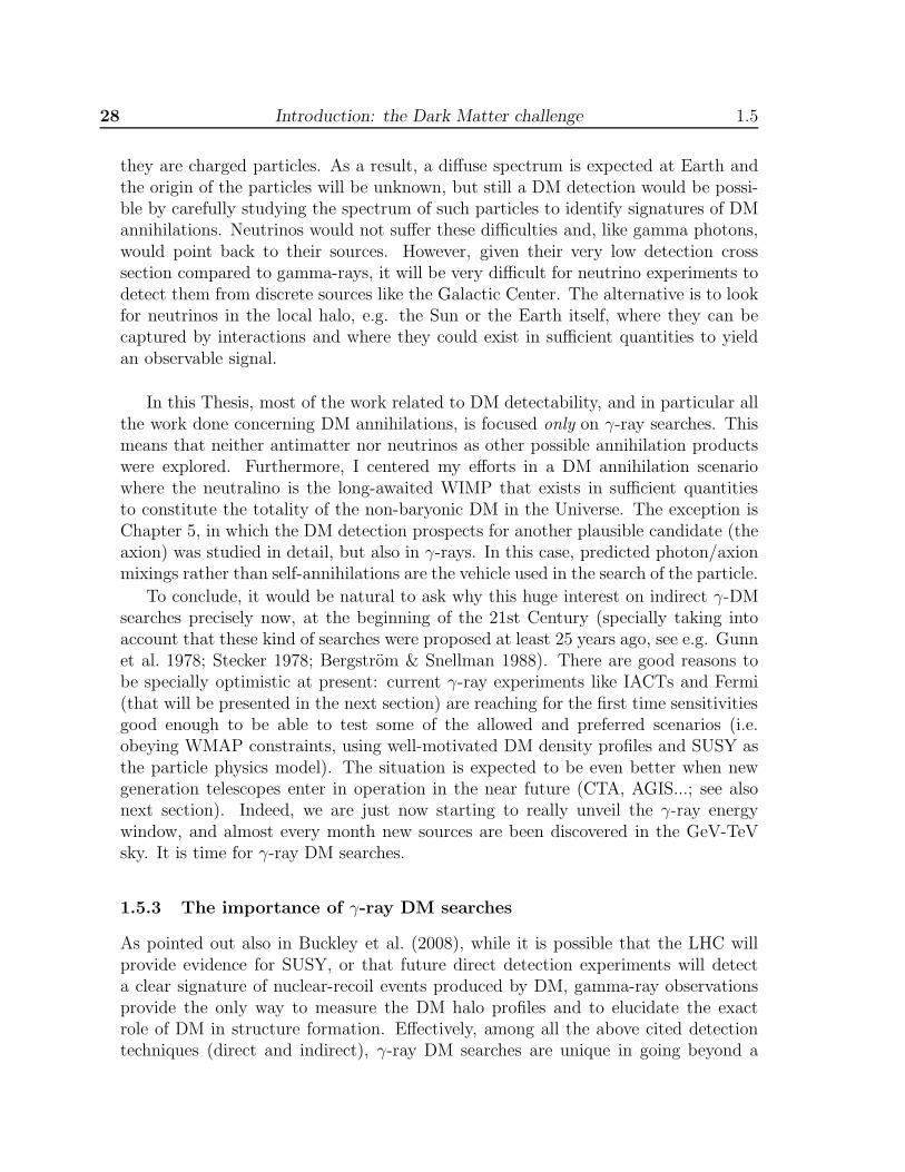
28 Introduction: the Dark Matter challenge 1.5
they are charged particles. As a result, a diffuse spectrum is expected at Earth andthe origin of the particles will be unknown, but still a DM detection would be possi-ble by carefully studying the spectrum of such particles to identify signatures of DMannihilations. Neutrinos would not suffer these difficulties and, like gamma photons,would point back to their sources. However, given their very low detection crosssection compared to gamma-rays, it will be very difficult for neutrino experiments todetect them from discrete sources like the Galactic Center. The alternative is to lookfor neutrinos in the local halo, e.g. the Sun or the Earth itself, where they can becaptured by interactions and where they could exist in sufficient quantities to yieldan observable signal.
In this Thesis, most of the work related to DM detectability, and in particular allthe work done concerning DM annihilations, is focused only on γ-ray searches. Thismeans that neither antimatter nor neutrinos as other possible annihilation productswere explored. Furthermore, I centered my efforts in a DM annihilation scenariowhere the neutralino is the long-awaited WIMP that exists in sufficient quantitiesto constitute the totality of the non-baryonic DM in the Universe. The exception isChapter 5, in which the DM detection prospects for another plausible candidate (theaxion) was studied in detail, but also in γ-rays. In this case, predicted photon/axionmixings rather than self-annihilations are the vehicle used in the search of the particle.
To conclude, it would be natural to ask why this huge interest on indirect γ-DMsearches precisely now, at the beginning of the 21st Century (specially taking intoaccount that these kind of searches were proposed at least 25 years ago, see e.g. Gunnet al. 1978; Stecker 1978; Bergstrom & Snellman 1988). There are good reasons tobe specially optimistic at present: current γ-ray experiments like IACTs and Fermi(that will be presented in the next section) are reaching for the first time sensitivitiesgood enough to be able to test some of the allowed and preferred scenarios (i.e.obeying WMAP constraints, using well-motivated DM density profiles and SUSY asthe particle physics model). The situation is expected to be even better when newgeneration telescopes enter in operation in the near future (CTA, AGIS...; see alsonext section). Indeed, we are just now starting to really unveil the γ-ray energywindow, and almost every month new sources are been discovered in the GeV-TeVsky. It is time for γ-ray DM searches.
1.5.3 The importance of γ-ray DM searches
As pointed out also in Buckley et al. (2008), while it is possible that the LHC willprovide evidence for SUSY, or that future direct detection experiments will detecta clear signature of nuclear-recoil events produced by DM, gamma-ray observationsprovide the only way to measure the DM halo profiles and to elucidate the exactrole of DM in structure formation. Effectively, among all the above cited detectiontechniques (direct and indirect), γ-ray DM searches are unique in going beyond a

1.6 The γ-ray energy window: IACTs, Fermi and future instruments 29
detection of the local halo to providing a measurement of the actual distribution ofDM in the Universe.
The general picture is that the LHC will be able to scan neutralino masses upto ∼300 GeV, well below the upper end of the allowed mass range. As for directdetection, WIMP-nucleon recoil experiments are most sensitive in the 60 to 600 GeVregime. Indirect DM searches below 100 GeV can be accomplished by the Fermi satel-lite and probably by MAGIC as well (see Section 1.6), while IACTs like MAGIC itselfor HESS should play a critical role for neutralino masses above 100 GeV. Therefore,and although direct detection and accelerator searches have an exciting discovery po-tential, there is a large region of parameter space for which gamma-ray instrumentscould provide the only detection (e.g. in case of nuclear recoil cross-section lies belowthe threshold of any planned direct detection experiment, or the mass is out of rangeof the LHC).
It seems clear that a combination of laboratory detection not only with direct butalso with indirect γ-ray DM searches will be required in order to successfully scanthe whole allowed SUSY parameter space, and to truly assess that a new particledetected by any of these methods really constitutes the enigmatic and long-awaitedto be discovered DM.
1.6 The γ-ray energy window: IACTs, Fermi and futureinstruments
1.6.1 Gamma-ray astrophysics in a nutshell
The cosmos and its evolution are studied using all radiation, in particular electro-magnetic waves. The observable spectrum extends from radio waves (at wavelengthsof several tens of meters, or energies of some 10−5 eV) to ultra-high energy gammaquanta (wavelengths of picometers or energies of 100 TeV). Observations at visiblewavelengths (0.5 to 1 micrometer) have a history of centuries, gamma astronomyby satellites (keV to few GeV) and ground-based telescopes (above 300 GeV) areend-of-20th century newcomers. Having no electric charge, gammas are not affectedby magnetic fields, and can, therefore, act as messengers of distant cosmic events,allowing straight extrapolation to the source. Indeed, high energy γ-rays combinethree characteristics that make these energetic photons ideal carriers of informationabout non-thermal relativistic processes in astrophysical settings (Aharonian 2004):(i) copious production in many galactic and extragalactic objects due to effectiveacceleration of charged particles and their subsequent interactions with the ambi-ent gas, low frequency radiation, and magnetic fields; (ii) free propagation in spacewithout deflection in the interstellar and intergalactic magnetic fields; (iii) effectivedetection by space-borne and ground based instruments. Therefore it is commonlybelieved that very high energy gamma-ray astronomy is destined to play a crucialrole in exploration of non-thermal phenomena in the Universe in their most extreme
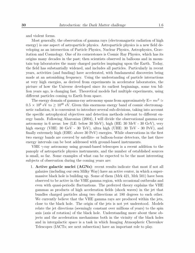
30 Introduction: the Dark Matter challenge 1.6
and violent forms.Most generally, the observation of gamma rays (electromagnetic radiation of high
energy) is one aspect of astroparticle physics. Astroparticle physics is a new field de-veloping as an intersection of Particle Physics, Nuclear Physics, Astrophysics, Grav-itation and Cosmology. One of its cornerstones is Cosmic Ray Physics, which has itsorigins many decades in the past; then scientists observed in balloons and in moun-tain top laboratories the many charged particles impinging upon the Earth. Today,the field has substantially widened, and includes all particles. Particularly in recentyears, activities (and funding) have accelerated, with fundamental discoveries beingmade at an astonishing frequency. Using the understanding of particle interactionsat very high energies, as derived from experiments in accelerator laboratories, thepicture of how the Universe developed since its earliest beginnings, some ten bil-lion years ago, is changing fast. Theoretical models fuel multiple experiments, usingdifferent particles coming to Earth from space.
The energy domain of gamma-ray astronomy spans from approximately E= mc2 ≃0.5 × 10⁶ eV to ≥ 1020 eV. Given this enormous energy band of cosmic electromag-netic radiation, it is convenient to introduce several sub-divisions, taking into accountthe specific astrophysical objectives and detection methods relevant to different en-ergy bands. Following Aharonian (2004), I will divide the observational gamma-rayastronomy in 6 areas: low (LE: below 30 MeV), high (HE: 30 MeV - 30 GeV), veryhigh energy (VHE: 30 GeV - 30 TeV), ultra high (UHE: 30 TeV - 30 PeV), andfinally extremely high (EHE: above 30 PeV) energies. While observations in the firsttwo energy bands are covered by satellite- or balloon-borne detectors, the last threeenergy intervals can be best addressed with ground-based instruments.
VHE γ-ray astronomy using ground-based telescopes is a recent addition to thepanoply of astroparticle physics instruments, and the number of established sourcesis small, so far. Some examples of what can be expected to be the most interestingsubjects of observation during the coming years are:
1. Active galactic nuclei (AGNs): recent results indicate that most if not allgalaxies (including our own Milky Way) have an active center, in which a super-massive black hole is building up. Some of them (Mrk 421, Mrk 501) have beenobserved to be active in the VHE gamma region, with occasional outbreaks andeven with quasi-periodic fluctuations. The preferred theory explains the VHEgammas as products of high acceleration fields (shock waves) in the jet thatbundles charged particles along two directions at 180 degrees to each other.We currently believe that the VHE gamma rays are produced within the jets,close to the black hole. The origin of the jets is not yet understood. Modelsrelate the jet directions (seemingly constant over millions of years) to the spinaxis (axis of rotation) of the black hole. Understanding more about these ob-jects and the acceleration mechanisms both in the vicinity of the black holesand in intergalactic space is a task in which Imaging Atmospheric CherenkovTelescopes (IACTs; see next subsection) have an important role to play.
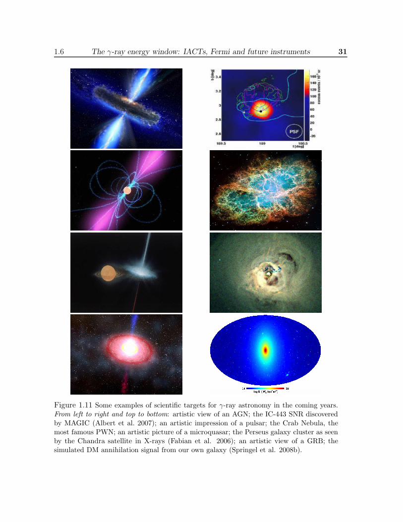
1.6 The γ-ray energy window: IACTs, Fermi and future instruments 31
Figure 1.11 Some examples of scientific targets for γ-ray astronomy in the coming years.From left to right and top to bottom: artistic view of an AGN; the IC-443 SNR discoveredby MAGIC (Albert et al. 2007); an artistic impression of a pulsar; the Crab Nebula, themost famous PWN; an artistic picture of a microquasar; the Perseus galaxy cluster as seenby the Chandra satellite in X-rays (Fabian et al. 2006); an artistic view of a GRB; thesimulated DM annihilation signal from our own galaxy (Springel et al. 2008b).

32 Introduction: the Dark Matter challenge 1.6
2. Supernova remnants: in the wake of a certain class of supernova explosions,the so-called SN of types II and Ia, gas clouds expand and a very dense coredevelops; the core may be a spinning neutron star or a black hole. Supernovaremnants may be VHE gamma sources of different types. According to the stan-dard model of cosmic ray origin, the shell type supernova remnants (radiatingfrom the expanding cloud) are sites of acceleration of nuclei to very high ener-gies: if so, they not only are the main accelerators of charged cosmic rays, butshould also copiously produce gamma rays. SN remnants of the plerion type,instead, are expected to radiate from the core. A systematic high-sensitivityscan of candidates, most of them lying in our own galaxy, has still to be done.
3. Sources found at lower energies but not yet identified: all-sky surveys ofwide-angle searching experiments in satellites have discovered a large number oflower energy gamma-ray emitters. The angular resolution of these detectors islimited, so that for more than half of these sources, it was not yet possible to re-late them to known sources observed at different wavelengths. The (third) 1999catalogue of sources established by the (no longer operating) EGRET detectoris a well-known book of astrophysics riddles: it lists 170 unidentified sources,along with 101 whose origin is thought to be understood. IACTs will collectmany more gamma rays from these sources, and thus pinpoint their positionsand contribute to their identification. The situation is now even more challeng-ing, since it is expected that the recently launched Fermi satellite discover a lotof new unidentified sources in gamma-rays that it will be necessary to study aswell.
4. Gamma Ray Bursts (GRBs): every day, a few powerful stellar explosionsilluminate the sky from all directions. Usually, they do not get recorded atvisible wavelengths, or only a very weak optical signal is seen. GRBs last forseconds to minutes only. Sometimes, an afterglow in the optical or X-ray do-main is observed after much longer delays. The energy observed makes themthe beacons of most likely the most energetic events known in the universe.Discovered 30 years ago, these GRBs have been objects for research and spec-ulation ever since. Today, a few thousand GRBs have been carefully charted,mostly by the BATSE satellite experiment. These objects cover the entire sky,seem spatially uncorrelated, many of them have large redshifts, i.e. we observethem at billions of years in the past, in the period of active star formation. Ob-servations in the VHE gamma domain are not available, so far, but are expectedto help clarifying these mysterious phenomena.
5. Other contributions to cosmology and fundamental physics: obser-vations of VHE gammas, if done systematically, will also allow to formulateconstraints on stellar formation in the early Universe, by measuring the ex-tragalactic infrared radiation field. They will further allow searches for the

1.6 The γ-ray energy window: IACTs, Fermi and future instruments 33
stable lightest supersymmetric particle, expected to annihilate with its ownself-conjugate antiparticle into gamma photons in areas of high gravitationalfield. Quantum gravity effects might become apparent if subtle time differ-ences can be detected in the arrival of gammas from a given source, at differentwavelengths.
Gamma-ray astronomy is currently under an extraordinary revolution, mainlydue to a battery of new instruments that has entered in operation in the last fewyears. From the ground, new generation Imaging Atmospheric Cherenkov Telescopes(IACTs) like MAGIC (Lorentz et al. 2004), HESS (Hinton et al. 2004), VERITAS(Weekes et al. 2002) or CANGAROO-III (Enomoto et al. 2002) have crucially con-tributed to revolutionize the field exploring the Universe above 50 GeV up to fewTeV, making possible the discovery of new gamma-ray sources, checking theoreticalscenarios on gamma-ray emission mechanisms in AGNs, imposing strong constraintsto cosmological models through observations of high redshift quasars, unveiling thenature of pulsars, etc. In space we have the small Italian satellite AGILE (Tavaniet al. 2008) and very specially Fermi (Gehrels & Michelson 1999; previously calledGLAST), in operation since Summer 2008 and covering energies in the range 0.02-300GeV. In the next subsections I will briefly review the present status of the field aswell as present gamma-ray experiments, both on the ground and out in space.
1.6.2 The imaging atmospheric Cherenkov technique. Present IACTs
IACTs are detectors for high-energy gamma quanta, installed on the surface of theEarth. The name Imaging Atmospheric Cherenkov Telescope (IACT) contains mostof the characteristics of this type of instrument:
1. The detectors have a light collection mirror and a camera, so they resembleoptical telescopes at least superficially.
2. These telescopes detect light produced by the Cherenkov effect, a radiationemitted by relativistic particles when being slowed down; the slowing down isin the atmosphere, where the high-energy gamma quanta get absorbed.
3. IACTs record many Cherenkov photons for a single original gamma; they areseen by the camera as an image whose characteristics allow to identify therecorded particle as a gamma, and to specify its direction and energy.
Because tha atmosphere has only narrow windows for wavelengths to pass, high-energy gamma rays do not reach the earth. They get absorbed in the atmosphere,transparent essentially only for visible and infrared light, and for long radio waves, asshown in Fig. 1.12. The absorption of the primary gamma leaves behind an avalanche,called an electromagnetic shower. The numerous secondary charged particles in sucha shower (for an incident gamma rather exclusively electrons and positrons) all radiate
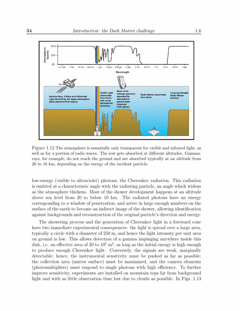
34 Introduction: the Dark Matter challenge 1.6
Figure 1.12 The atmosphere is essentially only transparent for visible and infrared light, aswell as for a portion of radio waves. The rest gets absorbed at different altitudes. Gamma-rays, for example, do not reach the ground and are absorbed typically at an altitude from20 to 10 km, depending on the energy of the incident particle.
low-energy (visible to ultraviolet) photons, the Cherenkov radiation. This radiationis emitted at a characteristic angle with the radiating particle, an angle which widensas the atmosphere thickens. Most of the shower development happens at an altitudeabove sea level from 20 to below 10 km. The radiated photons have an energycorresponding to a window of penetration, and arrive in large enough numbers on thesurface of the earth to become an indirect image of the shower, allowing identificationagainst backgrounds and reconstruction of the original particle’s direction and energy.
The showering process and the generation of Cherenkov light in a foreward conehave two immediate experimental consequences: the light is spread over a large area,typically a circle with a diameter of 250 m, and hence the light intensity per unit areaon ground is low. This allows detection of a gamma impinging anywhere inside thisdisk, i.e. an effective area of 30 to 105 m2, as long as the initial energy is high enoughto produce enough Cherenkov light. Conversely, the signals are weak, marginallydetectable; hence, the instrumental sensitivity must be pushed as far as possible:the collection area (mirror surface) must be maximized, and the camera elements(photomultipliers) must respond to single photons with high efficiency. To furtherimprove sensitivity, experiments are installed on mountain tops far from backgroundlight and with as little observation time lost due to clouds as possible. In Figs. 1.13
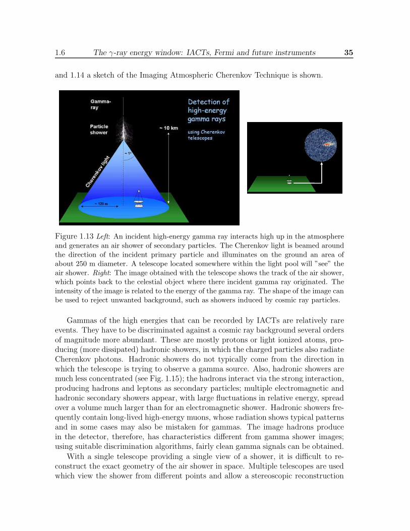
1.6 The γ-ray energy window: IACTs, Fermi and future instruments 35
and 1.14 a sketch of the Imaging Atmospheric Cherenkov Technique is shown.
Figure 1.13 Left: An incident high-energy gamma ray interacts high up in the atmosphereand generates an air shower of secondary particles. The Cherenkov light is beamed aroundthe direction of the incident primary particle and illuminates on the ground an area ofabout 250 m diameter. A telescope located somewhere within the light pool will ”see” theair shower. Right: The image obtained with the telescope shows the track of the air shower,which points back to the celestial object where there incident gamma ray originated. Theintensity of the image is related to the energy of the gamma ray. The shape of the image canbe used to reject unwanted background, such as showers induced by cosmic ray particles.
Gammas of the high energies that can be recorded by IACTs are relatively rareevents. They have to be discriminated against a cosmic ray background several ordersof magnitude more abundant. These are mostly protons or light ionized atoms, pro-ducing (more dissipated) hadronic showers, in which the charged particles also radiateCherenkov photons. Hadronic showers do not typically come from the direction inwhich the telescope is trying to observe a gamma source. Also, hadronic showers aremuch less concentrated (see Fig. 1.15); the hadrons interact via the strong interaction,producing hadrons and leptons as secondary particles; multiple electromagnetic andhadronic secondary showers appear, with large fluctuations in relative energy, spreadover a volume much larger than for an electromagnetic shower. Hadronic showers fre-quently contain long-lived high-energy muons, whose radiation shows typical patternsand in some cases may also be mistaken for gammas. The image hadrons producein the detector, therefore, has characteristics different from gamma shower images;using suitable discrimination algorithms, fairly clean gamma signals can be obtained.
With a single telescope providing a single view of a shower, it is difficult to re-construct the exact geometry of the air shower in space. Multiple telescopes are usedwhich view the shower from different points and allow a stereoscopic reconstruction
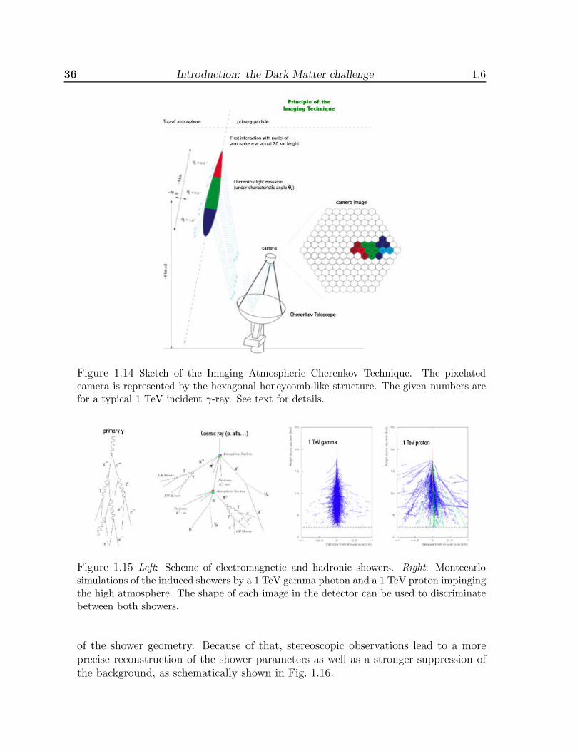
36 Introduction: the Dark Matter challenge 1.6
Figure 1.14 Sketch of the Imaging Atmospheric Cherenkov Technique. The pixelatedcamera is represented by the hexagonal honeycomb-like structure. The given numbers arefor a typical 1 TeV incident γ-ray. See text for details.
Figure 1.15 Left: Scheme of electromagnetic and hadronic showers. Right: Montecarlosimulations of the induced showers by a 1 TeV gamma photon and a 1 TeV proton impingingthe high atmosphere. The shape of each image in the detector can be used to discriminatebetween both showers.
of the shower geometry. Because of that, stereoscopic observations lead to a moreprecise reconstruction of the shower parameters as well as a stronger suppression ofthe background, as schematically shown in Fig. 1.16.

1.6 The γ-ray energy window: IACTs, Fermi and future instruments 37
Figure 1.16 Multiple telescopes are used to record the shower from different points andallow a stereoscopic reconstruction of the shower geometry. This kind of stereoscopic ob-servations provides a more precise reconstruction of the shower parameters as well as astronger suppression of the background.
The IACT was pioneered by the Whipple collaboration and led to the discoveryof TeV emission from the Crab Nebula in 1989. The Whipple 10m telescope alsodiscovered the first extra-galactic source of TeV emission with the detection of veryhigh energy gamma-ray emission from the active galaxy Markarian 421. The HEGRAtelescope array was the first system to use multiple telescopes, i.e. the stereoscopictechnique. Nowadays, the largest IACT telescope is the 17 m MAGIC telescope atthe Roque de los Muchachos Observatory in La Palma, which will be presented indetail is Section 7. However, as mentioned at the beginning of this section, there areat least other three IACTs which, together with MAGIC, lead the field above 100GeV at present: CANGAROO-III, HESS and VERITAS (see Figs. 1.17 and 1.18).
1.6.3 The Fermi satellite
The Fermi Gamma-ray Space Telescope (Fermi) satellite is a next generation high-energy gamma-ray observatory designed for making observations of celestial gamma-ray sources in the energy band extending from 10 MeV to more than 100 GeV. Itfollows in the footsteps of the CGRO-EGRET experiment, which was operationalbetween 1991 and 1999. Effectively, the Fermi Large Area Telescope (LAT), oneof the two instruments on board in the satellite (the other main instrument is the
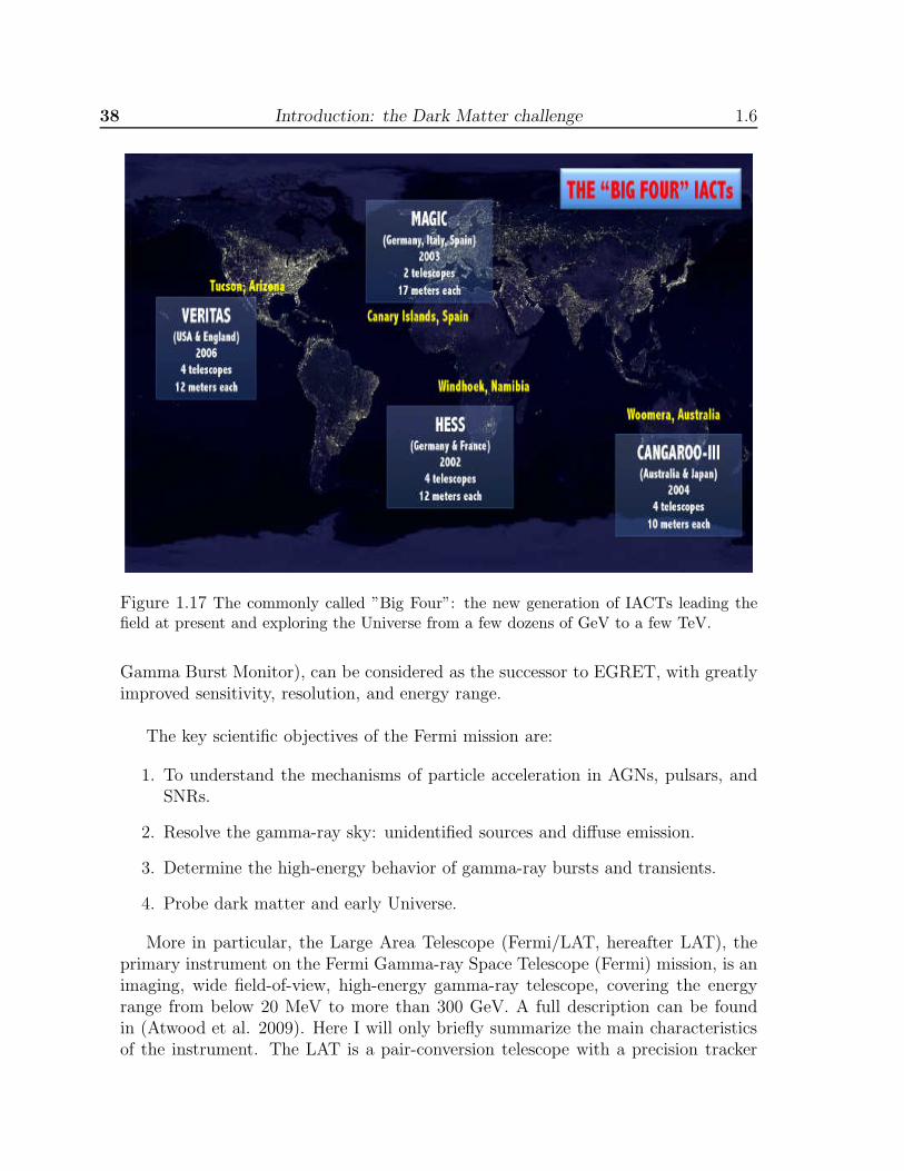
38 Introduction: the Dark Matter challenge 1.6
Figure 1.17 The commonly called ”Big Four”: the new generation of IACTs leading thefield at present and exploring the Universe from a few dozens of GeV to a few TeV.
Gamma Burst Monitor), can be considered as the successor to EGRET, with greatlyimproved sensitivity, resolution, and energy range.
The key scientific objectives of the Fermi mission are:
1. To understand the mechanisms of particle acceleration in AGNs, pulsars, andSNRs.
2. Resolve the gamma-ray sky: unidentified sources and diffuse emission.
3. Determine the high-energy behavior of gamma-ray bursts and transients.
4. Probe dark matter and early Universe.
More in particular, the Large Area Telescope (Fermi/LAT, hereafter LAT), theprimary instrument on the Fermi Gamma-ray Space Telescope (Fermi) mission, is animaging, wide field-of-view, high-energy gamma-ray telescope, covering the energyrange from below 20 MeV to more than 300 GeV. A full description can be foundin (Atwood et al. 2009). Here I will only briefly summarize the main characteristicsof the instrument. The LAT is a pair-conversion telescope with a precision tracker

1.6 The γ-ray energy window: IACTs, Fermi and future instruments 39
Figure 1.18 The “Big Four” again. From left to right and top to bottom: MAGIC, HESS,VERITAS and CANGAROO-III, the leading IACTs in the world at present.
and calorimeter. The tracking section has 36 layers of silicon microstrip detectorsto measure the tracks of charged particles, interleaved with 16 layers of tungstenfoil to promote γ-ray pair conversion. The tracker is followed by an array of CsIcrystals to determine the γ-ray energy and is surrounded by segmented charged-particle detectors (plastic scintillators with photomultiplier tubes) to reject cosmic-ray backgrounds. The LAT’s improved sensitivity compared to EGRET stems froma large peak effective area (∼8000 cm2, or ∼6 times greater than EGRET’s), largefield of view (∼2.4 sr, or nearly 5 times greater than EGRET’s), good backgroundrejection, superior angular resolution (68% containment angle ∼0.6 at 1 GeV forthe front section and about a factor of 2 larger for the back section), and improvedobserving efficiency (keeping the sky in the field of view with scanning observations).Pre-launch predictions of the instrument performance are described in Atwood et al.(2009). Verification of the on-orbit response is in progress but the indications arethat it is close to expectations. The sensitivity is about 50 times that of EGRET at100 MeV and even more at higher energies. Its two year limit for source detectionin an all-sky survey is 1.6 × 10⁻⁹ photons cm−2 s−1 (at energies > 100 MeV). It canlocate sources to positional accuracies of 30 arc seconds to 5 arc minutes, depending
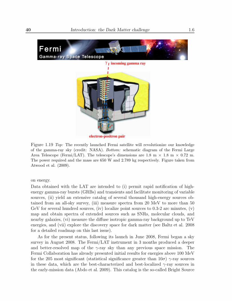
40 Introduction: the Dark Matter challenge 1.6
Figure 1.19 Top: The recently launched Fermi satellite will revolutionize our knowledgeof the gamma-ray sky (credit: NASA). Bottom: schematic diagram of the Fermi LargeArea Telescope (Fermi/LAT). The telescope’s dimensions are 1.8 m × 1.8 m × 0.72 m.The power required and the mass are 650 W and 2.789 kg respectively. Figure taken fromAtwood et al. (2009).
on energy.
Data obtained with the LAT are intended to (i) permit rapid notification of high-energy gamma-ray bursts (GRBs) and transients and facilitate monitoring of variablesources, (ii) yield an extensive catalog of several thousand high-energy sources ob-tained from an all-sky survey, (iii) measure spectra from 20 MeV to more than 50GeV for several hundred sources, (iv) localize point sources to 0.3-2 arc minutes, (v)map and obtain spectra of extended sources such as SNRs, molecular clouds, andnearby galaxies, (vi) measure the diffuse isotropic gamma-ray background up to TeVenergies, and (vii) explore the discovery space for dark matter (see Baltz et al. 2008for a detailed roadmap on this last issue).
As for the present status, following its launch in June 2008, Fermi began a skysurvey in August 2008. The Fermi/LAT instrument in 3 months produced a deeperand better-resolved map of the γ-ray sky than any previous space mission. TheFermi Collaboration has already presented initial results for energies above 100 MeVfor the 205 most significant (statistical significance greater than 10σ) γ-ray sourcesin these data, which are the best-characterized and best-localized γ-ray sources inthe early-mission data (Abdo et al. 2009). This catalog is the so-called Bright Source

1.6 The γ-ray energy window: IACTs, Fermi and future instruments 41
o-180o+180
o+90
o-90
Crab/Crab Pulsar
Mkn 421
Mkn 501
2344+514
1959+650
PSR 1706
2155-304
Cas A
1426+428 M87
BL LacTeV 2032+4130
Vela
RX J1713PSR 1259-63
Sgr A*
G0.9+0.1
PSR 1509-58
2005-489HESS J1614-518
HESS J1616-508
HESS J1640-465
HESS J1804-216
HESS J1813-178
HESS J1825-137
HESS J1834-087
HESS J1837-069
1218+304
1553+113
HESS J1303-631
MSH 15-52
LS I+61
Mkn 180
LS 5039
1101-232
2356-309
HESS J0832+058
HESS J1632-478
HESS J1634-472
HESS J1702-420
HESS J1708-410
HESS J1713-381
HESS J1745-303
HESS J1418-609
HESS J1420-607
HESS J1718-385
HESS J1809-193Westerlund 2
0548-322
0229+200
0347-121
HESS J1912+101
W 28
MAGIC J0616+025
Cygnus X-1
1011+496
RCW 86
3C 279
MGRO J1908+06
MGRO J2031+41
MGRO J2019+37
Kes 75
G21.5-0.9 HESS J0632+057
HESS J1718-385
HESS J1809-193
HESS J1357-645
HESS J1427-608
HESS J1626-490
HESS J1702-420
HESS J1708-410
HESS J1731-347
HESS J1841-055HESS J1857+026
0152+017
0806+524
W Comae
S5 0716+71
SN 1006
3C 66A
Cen A
0710+591
-ray sourcesγVHE
Blazar (HBL)Blazar (LBL)
Flat Spectrum Radio QuasarRadio Galaxy
Pulsar Wind NebulaSupernova RemnantBinary System
Open Cluster
Unidentified
-ray Sky MapγVHE >100 GeV)γ(E
2009-02-25 - Up-to-date plot available at http://www.mppmu.mpg.de/~rwagner/sources/
Figure 1.20 Top: The EGRET all-sky map above 100 MeV (left) and the Third (and final)EGRET Catalog of detected sources (right) (Credit: EGRET team). Middle: The Fermiall-sky map after 3 months of operation (left) and the corresponding 205 Fermi BrightSource Catalog (right) (Credit: Fermi team). Bottom: The TeV sky as of early 2003 (left),with only 17 sources known; since then, a lot of new sources have been discovered with thenew generation IACTs, as can be clearly seen in the updated version of this map above 100GeV (right).
Catalog (BSC), although the first official LAT catalog is planned for release after thefirst year of operations. In FIg. 1.20 the sources of the BSC are shown in an all-skymap. The Third EGRET Catalog is also shown as comparison in the same Figure,as well as an all-sky map of detected sources at even higher energies (>100 GeV). Inaddition to this important new γ-ray catalog, there are other Fermi highlights, like

42 Introduction: the Dark Matter challenge 1.6
the measurement of the Cosmic Ray e++e− spectrum from 20 GeV to 1 TeV (Abdoet al. 2009b) or the discovery of new pulsars and AGNs (see e.g. Abdo et al. 2008and Abdo et al. 2009c respectively).
1.6.4 Planned instruments for the near future
There are essentially two enormous efforts under way to improve the IACT capabilitiesfor the next decade: the Cherenkov Telescope Array, or CTA, which is essentially anEuropean effort, and the Advanced Gamma-ray Imaging System (AGIS), which isthe analogous in the U.S.
The Cherenkov Telescope Array (CTA) is an European project to build a newgeneration ground-based γ-ray instrument that operates in the energy rangeextending from some tens of GeV to above 100 TeV. It is conceived as an openobservatory and will consist of two arrays of IACTs: a first one at the NorthernHemisphere which will preferentially study extragalactic objects at the lowestpossible energies; a second array at the Southern Hemisphere to cover the fullenergy range and specially concentrate on galactic sources. The CTA scientificobjectives go beyond high energy astrophysics into Cosmology and FundamentalPhysics. A more detailed description of the project can be found in Martınez(2008)4.
CTA intends to improve the flux sensitivity of the current generation of IACTssuch as MAGIC, HESS and VERITAS by an order of magnitude. Althoughthe exact design of CTA is being studied and not precisely defined as of now,a possible design could be a combination of arrays of 2-3 different telescopesizes. A large number (several tens) of mid-size telescopes will provide forthe millicrab sensitivity and high angular resolution (up to a factor ∼5 thanpresent IACTs) in the core energy range from about 100 GeV up to 10 TeV. Anextension of a few (4-9) very large diameter telescopes and many (up to 100)very small telescopes distributed over a large area enlarge the energy range fromseveral 10 GeV up to 100 TeV. A sketch of the design is shown in Fig. 1.21. Theproject could be running as early as 2015, although this date is very dependenton funding.
The Advanced Gamma-ray Imaging System (AGIS) is a next-generationground-based γ-ray observatory being planned in the U.S. The AGIS projectmirrors the CTA project being discussed in Europe. As CTA, it is expected thatAGIS will improve the sensitivity of current IACTs by one order of magnitude.AGIS will also have substantially improved angular resolution, which will con-strain the origin of detected gamma-rays more tightly, enabling astronomersto better model the mechanisms responsible for emission. The energy range
4or you can also visit the CTA website: http://www.cta-observatory.org
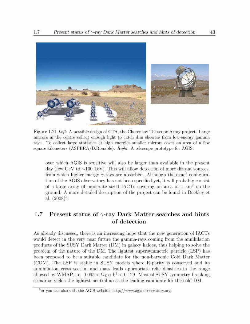
1.7 Present status of γ-ray Dark Matter searches and hints of detection 43
Figure 1.21 Left: A possible design of CTA, the Cherenkov Telescope Array project. Largemirrors in the centre collect enough light to catch dim showers from low-energy gammarays. To collect large statistics at high energies smaller mirrors cover an area of a fewsquare kilometers (ASPERA/D.Rouable). Right: A telescope prototype for AGIS.
over which AGIS is sensitive will also be larger than available in the presentday (few GeV to ∼100 TeV). This will allow detection of more distant sources,from which higher energy γ-rays are absorbed. Although the exact configura-tion of the AGIS observatory has not been specified yet, it will probably consistof a large array of moderate sized IACTs covering an area of 1 km2 on theground. A more detailed description of the project can be found in Buckley etal. (2008)5.
1.7 Present status of γ-ray Dark Matter searches and hints
of detection
As already discussed, there is an increasing hope that the new generation of IACTswould detect in the very near future the gamma-rays coming from the annihilationproducts of the SUSY Dark Matter (DM) in galaxy haloes, thus helping to solve theproblem of the nature of the DM. The lightest supersymmetric particle (LSP) hasbeen proposed to be a suitable candidate for the non-baryonic Cold Dark Matter(CDM). The LSP is stable in SUSY models where R-parity is conserved and itsannihilation cross section and mass leads appropriate relic densities in the rangeallowed by WMAP, i.e. 0.095 < ΩDM h2 < 0.129. Most of SUSY symmetry breakingscenarios yields the lightest neutralino as the leading candidate for the cold DM.
5or you can also visit the AGIS website: http://www.agis-observatory.org

44 Introduction: the Dark Matter challenge 1.7
In the Lambda Cold Dark Matter (ΛCDM) paradigm, which represents the mostaccepted cosmological scenario at present (see Section 1.2), around 23% of the Uni-verse consists of non-barionic Dark Matter (DM). This kind of DM is needed in orderto explain a large amount of astrophysical processes at all scales, such as the for-mation of structures in the early Universe, their evolution with time so that theycan form the structures observable today, the results from gravitational lensing, therotation curves of individual galaxies, etc (Section 1.1). To be able to explain theseastrophysical puzzles, the DM particles should interact very weakly with the ordinarymatter and should have low thermal velocities (Section 1.4.2). A very good candi-date is the neutralino, that fulfill the above mentioned characteristics and arises inthe context of SUSY (SuperSymmetry, the most preferred Particle Physics scenariobeyond the Standard Model, briefly presented in Section 1.4.2 as well). An inter-esting property of the neutralino is that it is predicted to be its own antiparticle,which means that it will annihilate when interacting with other neutralinos. Thisfact is crucial for detectability purposes and represents indeed the main vehicle usedat present in DM searches. One of the products of these annihilations are predictedto be gamma-rays (Section 1.5.2), whose specific energy will vary according to thechosen particle physics model, but that is expected to lie in the energy range coveredby the current Imaging Atmospheric Cherenkov Telescopes (IACTs) like CANGA-ROO, HESS, MAGIC and VERITAS (Section 1.6.2). The DM annihilation flux isproportional to the square DM density, which means that the best places to searchfor DM in the Universe are those with the highest expected DM densities. Distance isalso very important, since high DM dominated systems that are located too far fromus will yield too low DM annihilation fluxes at Earth. Having both considerationsin mind, it is clear that the Galactic Center should be a very good candidate, butalso dwarf spheroidal galaxies satellites of the Milky Way, and nearby galaxy clustersarise as very good candidates for DM searches.
At present, different astrophysical objects (the Galactic Center, galaxy clusters,dwarf galaxies) have been observed in γ-rays and studied in the context of DMsearches. These observations were mainly carried out by current IACTs from theground, like MAGIC or HESS. As known, no clear signal from DM annihilation hasbeen found yet (at least unequivocal). Here I will briefly review the present statusof DM searches, although some of them will be discussed more in detail in otherChapters of this Thesis (in particular MAGIC observations of dwarfs).
• Galactic Center: In principle, the best option for DM searches seems to bethe Galactic Centre (GC), since a high DM concentration is expected thereand it is also very near compared to other potential targets. However, theGC is a very crowded region, which makes it difficult to discriminate betweena possible γ-ray signal due to neutralino annihilation and other astrophysicalsources. Whipple (Kosack et al. 2004), CANGAROO (Tsuchiya et al. 2004),
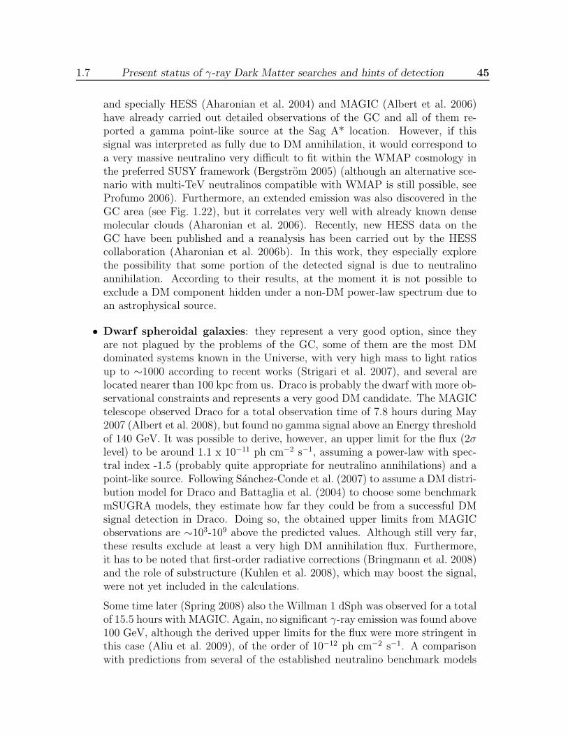
1.7 Present status of γ-ray Dark Matter searches and hints of detection 45
and specially HESS (Aharonian et al. 2004) and MAGIC (Albert et al. 2006)have already carried out detailed observations of the GC and all of them re-ported a gamma point-like source at the Sag A* location. However, if thissignal was interpreted as fully due to DM annihilation, it would correspond toa very massive neutralino very difficult to fit within the WMAP cosmology inthe preferred SUSY framework (Bergstrom 2005) (although an alternative sce-nario with multi-TeV neutralinos compatible with WMAP is still possible, seeProfumo 2006). Furthermore, an extended emission was also discovered in theGC area (see Fig. 1.22), but it correlates very well with already known densemolecular clouds (Aharonian et al. 2006). Recently, new HESS data on theGC have been published and a reanalysis has been carried out by the HESScollaboration (Aharonian et al. 2006b). In this work, they especially explorethe possibility that some portion of the detected signal is due to neutralinoannihilation. According to their results, at the moment it is not possible toexclude a DM component hidden under a non-DM power-law spectrum due toan astrophysical source.
• Dwarf spheroidal galaxies: they represent a very good option, since theyare not plagued by the problems of the GC, some of them are the most DMdominated systems known in the Universe, with very high mass to light ratiosup to ∼1000 according to recent works (Strigari et al. 2007), and several arelocated nearer than 100 kpc from us. Draco is probably the dwarf with more ob-servational constraints and represents a very good DM candidate. The MAGICtelescope observed Draco for a total observation time of 7.8 hours during May2007 (Albert et al. 2008), but found no gamma signal above an Energy thresholdof 140 GeV. It was possible to derive, however, an upper limit for the flux (2σlevel) to be around 1.1 x 10⁻¹¹ ph cm−2 s−1, assuming a power-law with spec-tral index -1.5 (probably quite appropriate for neutralino annihilations) and apoint-like source. Following Sanchez-Conde et al. (2007) to assume a DM distri-bution model for Draco and Battaglia et al. (2004) to choose some benchmarkmSUGRA models, they estimate how far they could be from a successful DMsignal detection in Draco. Doing so, the obtained upper limits from MAGICobservations are ∼103-109 above the predicted values. Although still very far,these results exclude at least a very high DM annihilation flux. Furthermore,it has to be noted that first-order radiative corrections (Bringmann et al. 2008)and the role of substructure (Kuhlen et al. 2008), which may boost the signal,were not yet included in the calculations.
Some time later (Spring 2008) also the Willman 1 dSph was observed for a totalof 15.5 hours with MAGIC. Again, no significant γ-ray emission was found above100 GeV, although the derived upper limits for the flux were more stringent inthis case (Aliu et al. 2009), of the order of 10−12 ph cm−2 s−1. A comparisonwith predictions from several of the established neutralino benchmark models
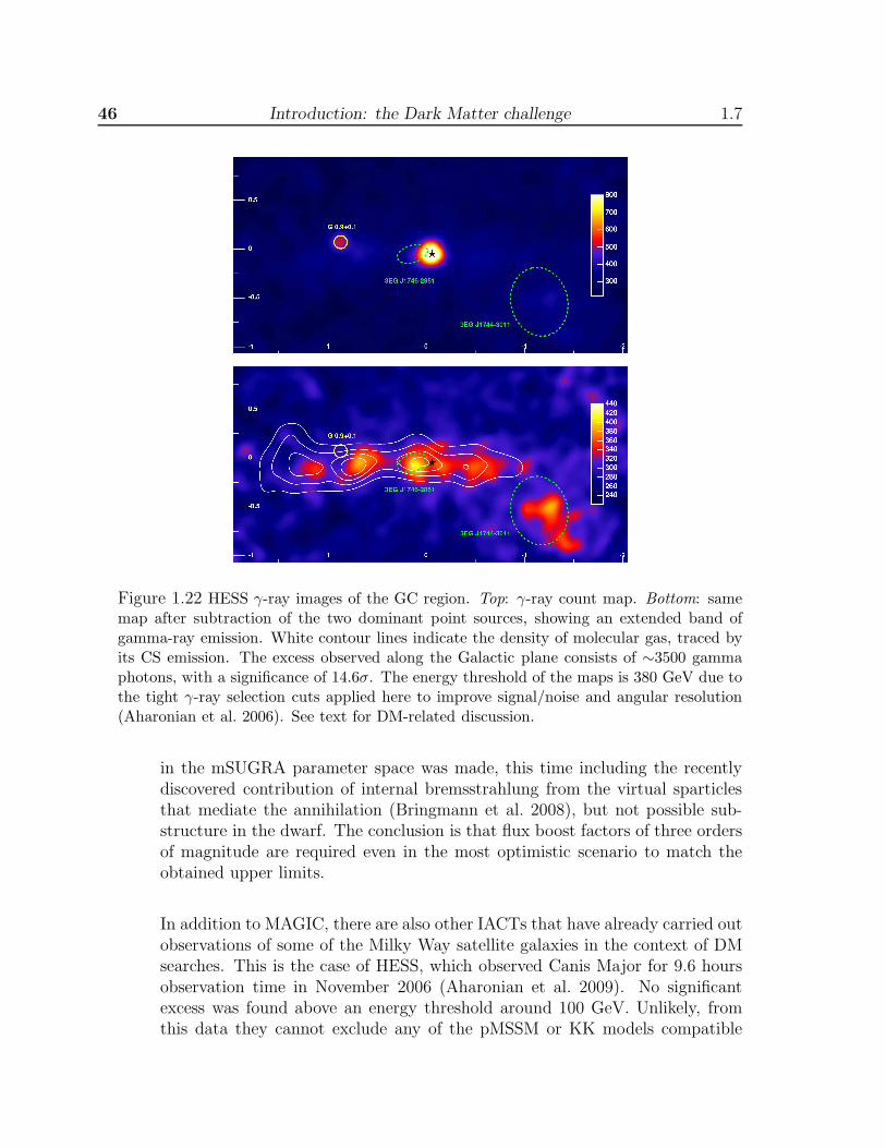
46 Introduction: the Dark Matter challenge 1.7
Figure 1.22 HESS γ-ray images of the GC region. Top: γ-ray count map. Bottom: samemap after subtraction of the two dominant point sources, showing an extended band ofgamma-ray emission. White contour lines indicate the density of molecular gas, traced byits CS emission. The excess observed along the Galactic plane consists of ∼3500 gammaphotons, with a significance of 14.6σ. The energy threshold of the maps is 380 GeV due tothe tight γ-ray selection cuts applied here to improve signal/noise and angular resolution(Aharonian et al. 2006). See text for DM-related discussion.
in the mSUGRA parameter space was made, this time including the recentlydiscovered contribution of internal bremsstrahlung from the virtual sparticlesthat mediate the annihilation (Bringmann et al. 2008), but not possible sub-structure in the dwarf. The conclusion is that flux boost factors of three ordersof magnitude are required even in the most optimistic scenario to match theobtained upper limits.
In addition to MAGIC, there are also other IACTs that have already carried outobservations of some of the Milky Way satellite galaxies in the context of DMsearches. This is the case of HESS, which observed Canis Major for 9.6 hoursobservation time in November 2006 (Aharonian et al. 2009). No significantexcess was found above an energy threshold around 100 GeV. Unlikely, fromthis data they cannot exclude any of the pMSSM or KK models compatible
1.7 Present status of γ-ray Dark Matter searches and hints of detection 47
with WMAP+SDSS constraints. They derived, however, an upper limit for themass of this dwarf to be around 109 M⊙. HESS also observed Sagittarius for11 hours exposure time in June 2006 (Aharonian et al. 2008). No significantexcess was found above Eth >250 GeV, although they claimed the exclusion ofsome pMSSM models from the data assuming a core DM density profile for thisgalaxy. The Whipple IACT also observed two galaxy satellites during 2003:Draco (14.3 h) and UMi (17.2 h). Again, no significant excess was found above400 GeV, and it was not possible to rule out any of the MSSM allowed modelsfrom these observations (Wood et al. 2008).
The MAGIC observational campaigns carried out in the context of DM searchesfor Draco and Willman 1 constitute an essential part of this Thesis, since I wasinvolved both in the data acquisition and in the theoretical interpretation ofthe data. Therefore, they will be presented in detail in Chapters 8 (Draco) and9 (Willman 1).
• Galaxy clusters: Clusters of galaxies are the largest and most massive grav-itationally bound systems in the Universe, with masses of 1014-1015 M⊙, ofwhich galaxies, gas and DM contribute roughly 5, 15 and 80 %, respectively(see e.g. Sarazin (1988) for a review). This makes them very attractive also inDM searches, despite the fact that they are not as near as other potential DMcandidates. While no cluster has been firmly detected as a gamma-ray sourceso far, they are expected to be significant gamma-ray emitters for conventionalphysical processes. For DM purposes, it will be necessary to understand and tomodel this non-exotic emission in order to discriminate it from a possible DMannihilation signal. Some galaxy cluster observations have been performed bysome of the IACTs currently in operation, but only poor upper limits have beenobtained. For example, those coming from the HESS Collaboration for Coma,Abell 496 (Domainko et al. 2008), and Abel 85 (Aharonian et al. 2009b); fromVERITAS for Coma (Perkins 2008) and from Whipple for Perseus and Abell2029 (Krawczynski et al. 2005). All of them were preceded by EGRET upperlimits at lower energies (Reimer et al. 2003).
There are also other proposed DM scenarios in the literature that still lack gammaobservations, like Milky Way substructure (for which Fermi could be specially rele-vant), nearby microhalos (again more readily accessible to Fermi), Intermediate MassBlack Holes (IMBHs), etc.
In conclusion, there is no conclusive evidence of DM annihilation at present, butthere have been several claims of discovery in the last few years, or at least hints ofDM detection, coming from different DM search strategies rather than those basedon γ-rays (note that, in γ-rays, certainly the Galactic Center observations may beconsidered as a hint, although as discussed above a DM interpretation of the data

48 Introduction: the Dark Matter challenge 1.7
is strongly disfavored by the most preferred theoretical models). Below I will brieflydiscuss some of them (I refer to Hooper 2009 for an excellent and updated review oneach of them):
1. The PAMELA and ATIC Excesses: The PAMELA experiment recently re-ported an unexpected anomaly in the positron to positron-plus-electron ratioabove 10 GeV (Adriani et al. 2009), in this way confirming previous claims fromHEAT (Coutu et al. 2001) and AMS-01 (Olzem et al. 2006). Also recently, theATIC balloon experiment has published a feature between ∼300-800 GeV inthe cosmic ray electron (plus positron) spectrum, with a maximum ∼600 GeV.In addition to both excesses, WMAP data from the central region of our galaxyseems to point to an excess of microwave emission that can be interpreted asdue synchrotron emission coming from a population of electron and positronswith a hard spectral index (e.g. Hooper et al. 2007). All these observationstaken together seemed to point to essentially one of the following interpreta-tions: (1) emission from pulsars (e.g. Profumo 2008) or DM annihilations (e.g.Bergstrom et al. 2009). Certainly, although the data could be explained by thelatter possibility, the an annihilation rate should be many hundred times largerthan typically expected, and should need a rather special DM distribution aswell. Therefore, at present, the most plausible explanation of this excess isan scenario where its origin is a nearby pulsar or pulsars. It is important tonote here, however, that very recently Fermi also published relevant data inthis discussion: Fermi does not confirm the ATIC excess (Abdo et al. 2009b).Also the HESS collaboration reported data above 340 GeV in the cosmic rayelectron spectrum (Aharonian et al. 2009c). The H.E.S.S. data with their lowerstatistical errors show no indication of a structure in the electron spectrum, butrather a power-law spectrum. This makes the situation even more difficult toclarify (see Fig. 1.23).
2. The WMAP Haze: In addition to detailed CMB maps, data from WMAP hasalso provided critical information on the standard interstellar medium mecha-nisms. These observations have revealed an excess of microwave emission 20
around the Galactic Center, more or less with radial symmetry, known as “theWMAP haze” (Dobler & Finkbeiner 2008). One of the possible explanationsis DM annihilation (Hooper et al. 2007; Caceres 2009). Again, Fermi shouldplay a crucial role to dilucidate the real origin of this excess, specially takinginto account that, according to recent works, the annihilation cross section aswell as the DM density profile needed to reproduce the WMAP haze imply agamma-ray flux that should be observed by this satellite (Hooper et al. 2008).
3. DAMA Annual Modulation: recently, this DM direct detection experiment re-ported evidence for an annual modulation (at 8σ level) in its rate of nuclearrecoils that could be interpreted as due to WIMP interactions with ordinary

1.7 Present status of γ-ray Dark Matter searches and hints of detection 49
Energy (GeV)1 10 100
))
-(eφ
)+
+(eφ
) / (
+(eφ
Po
sitr
on
fra
ctio
n
0.01
0.02
0.1
0.2
0.3
PAMELA
Figure 1.23 Left: The PAMELA positron fraction compared with the theoretical model(Adriani et al. 2009). Right: The Fermi LAT cosmic ray electron spectrum (red filledcircles). Systematic errors are shown by the gray band. Other high-energy measurementsand a conventional diffusive model are shown (Abdo et al. 2009b).
matter (Bernabei et al. 2008). The DAMA Collaboration excluded any system-atics that could be producing the measured signal. However, this DM detectionclaim is very controversial, since other experiments that are currently scanningthe same region of the DAMA parameter space could not find the same evi-dence. This point was already previously discussed in Section 1.5.1.
4. The INTEGRAL 511 keV Line: in 2003, the INTEGRAL satellite confirmeda bright emission of 511 keV photons from the region of the Galactic Bulgeapproximately spherically symmetric (∼6 diameter). This signal is some ordersof magnitude larger than expected from pair creation via cosmic ray interactionswith the interstellar medium (Jean et al. 2003). Therefore, given the difficultiesto explain this emission with conventional astrophysical sources, some worksappeared that proposed a DM annihilation origin (Boehm et al. 2004). If thiswas the case, the DM particle should have a mass in the range 1-3 MeV, i.e.the so-called Light DM.
5. EGRET Diffuse Galactic Spectrum: an excess of gamma-rays seems to bepresent also in EGRET data collected from the whole sky above approximately1 GeV, which has been interpreted as an evidence of DM annihilations in theMilky Way halo (e.g. de Boer et al. 2005). The data would imply a WIMPmass ∼50-100 GeV, although this interpretation is not exempt of several diffi-culties. Preliminary data from the Fermi satellite, however, does not supportthis excess. More Fermi observations are needed in order to definitely clarifythe situation.
50 Introduction: the Dark Matter challenge 1.7
6. EGRET Diffuse Extragalactic Spectrum: it exists the possibility that a portionof the measured EGRET extragalactic diffuse gamma-ray flux could be dueto DM annihilations taking place throughout the Universe (e.g. Elsaesser &Mannheim 2005). Indeed, EGRET data fits quite well with WIMP massesaround 500 GeV. The DM annihilation rate, however, seems to be quite high ifcompared to what it is expected from the most preferred particle physics andastrophysical models. More data is also needed, specially from Fermi.
Bibliography
Aalseth C. E., et al., 2008, Phys. Rev. Lett., 101, 251301
Abazajian K., Fuller G. M. and Patel M., 2001, Phys. Rev. D, 64, 023501
Abdo A. A., et al. [Fermi collaboration], 2008, Science, 322, 1218
Abdo, A. A., et al., 2009, ApJS, 183, 46
Abdo A. A., et al. [Fermi collaboration], 2009b, Phys. Rev. Lett., 102, 181101
Abdo A. A., et al. [Fermi collaboration], 2009c, ApJ, 697, 934
Adelman-McCarthy, J. K., et al. 2006, ApJS, 162, 38
Adriani O., et al., 2009, Nature, 458, 607
Aharonian F. A., 2004, Very High Energy Cosmic Gamma radiation, World ScientificPublishing Co., Singapore
Aharonian F. et al., [HESS Collaboration], 2004, A&A, 425, L13
Aharonian F. et al., [HESS Collaboration], 2006, Nature, 439, 695
Aharonian F. et al., [HESS Collaboration], 2006b, Phys. Rev. Lett., 97, 221102
Aharonian, F., et al., [HESS Collaboration], 2008, Astroparticle Physics, 29, 55
Aharonian F. et al., [HESS Collaboration], 2009, ApJ, 691, 175
Aharonian, F. et al., [HESS Collaboration], 2009b, A&A, 495, 27
Aharonian, F. et al., [HESS Collaboration], 2009c, arXiv:0905.0105
Ahmed, Z., et al. 2009, Phys. Rev. Lett., 102, 011301
Akerib D. S., et al., 2003, Phys. Rev. D, 68, 082002
52 BIBLIOGRAPHY 1.7
Albert J., et al. [MAGIC collaboration], 2006, ApJ, 638, L101
Albert J., et al. [MAGIC collaboration], 2008, ApJ, 679, 428
Aliu J., et al. [MAGIC collaboration], 2009, ApJ, 695, 1
Alcock C., et al. 2000, ApJ, 542, 281
Alner G. J., et al., 2007, Astropart. Phys. 28, 287
Amati L., 2006, Mon. Not. Roy. Astron. Soc. 372, 233
Angle J., et al., [XENON Collaboration], 2008, Phys. Rev. Lett. 100, 021303
Angloher G., et al., Astropart. Phys. 2005, 23, 325
Ansari R., et al., 2004, arXiv:astro-ph/0407583
Atwood W. B., et al. [Fermi collaboration], 2009, ApJ, 697, 1071
J. Bagla, 2005, Curr. Sci. 88, 1088
Bahcall, J. N., Flynn, C., and Gould, A. 1992, ApJ, 389, 234
Bahcall N. and Fan X., 1998, ApJ, 504, 1
Baltz E. A. et al., 2004, arXiv:astro-ph/0412170
Baltz E. A. et al., 2008, JCAP, 7, 013
Battaglia, M., et al., 2004, European Phys. J. C, 33, 273
Begeman K. G., Broeils A. H. and Sanders R. H., 1991, MNRAS, 249, 523
Behnke E., et al. [COUPP Collaboration], Science, 319, 933
Bekenstein J. and Milgrom M., 1984, ApJ, 286, 7
Bekenstein J.D., 1988, Phys. Lett. B, 202, 497
Bekenstein, J. D., 2004, Phys.Rev. D, 70, 083509
Benetti et al. [Warp Collaboration], et al. 2008, Astroparticle Physics, 28, 495
Benoit A. et al., 2002, Phys. Lett. B, 545, 43
Bergstrom L. and Snellman H., Phys. Rev. D, 1988, 37, 3737
Bergstrom, L., Ullio, P., & Buckley, J. H., 1998, Astroparticle Physics, 9, 137

1.7 BIBLIOGRAPHY 53
Bergstrom, L. 2000, Reports on Progress in Physics, 63, 793
Bergstrom L. et al., 2005, Phys. Rev. Lett., 95, 241301
Bergstrom, L., Edsjo, J., & Zaharijas, G. 2009, arXiv:0905.0333
Bernabei R., et al. [DAMA Collaboration], 2008, Eur.Phys.J., C56, 333
Bertone, G., Hooper, D., & Silk, J. 2005, Phys. Reports, 405, 279
Bertone, G., 2007, Astrophys. Space Sci., 309, 505
Binetruy P., Gaillard M.K. and Nelson B.D., 2001, Nucl. Phys. B, 604, 32
Boehm C., Hooper D., Silk J., Casse M. and Paul J., Phys. Rev. Lett., 2004, 92,101301
Bond J.R., Efstathiou G. and Silk J., 1980, Phys. Rev. Lett., 45, 1980
Briel, U.G. and Henry, J.P., 2007, arXiv:astro-ph/9711237
Bringmann, T., Bergstrom, L., & Edsjo, J. 2008, JHEP, 1, 49
Broadhurst T., Umetsu K., Medezinski E., Oguri M. and Rephaeli Y., 2008, ApJ,685, L9
Buckley J. et al., 2008, Procs. of the 4th International Meeting on High EnergyGamma-Ray Astronomy, AIP Conf. Procs., 1085, 902-905
Buckley J. et al., 2008, Report from the Dark Matter Science Working group ofthe APS commissioned White paper on ground-based TeV gamma ray astronomy,arXiv:astro-ph/0812.0795
Bullock, J. S., Dekel, A., Kolatt, T. S., Kravtsov, A. V., Klypin, A. A., Porciani,C., & Primack, J. R. 2001, ApJ, 555, 240
J. S. Bullock, K. R. Stewart and C. W. Purcell, 2008, IAU Symposium 254, TheGalaxy Disk in Cosmological Context, arXiv:0811.0861
Caceres, G., 2009, SnowPAC 2009 conference proceeding, to appear in ASP Confer-ence Series, arXiv:0906.4306
Carlberg R.G. et al., 1999, ApJ, 516, 552
Choi K.Y. and Roszkowski L., 2006, AIP Conf.Proc., 805, 30
Clowe, D., et al., 2006, ApJ, 648, L109
Cole, S., et al. 2005, Mon. Not. Roy. Astron. Soc., 362, 505
54 BIBLIOGRAPHY 1.7
Copeland E.J., Sami M. and Tsujikawa S., 2006, Int. J. Mod. Phys. D 15, 1753
Coutu S., et al. [HEAT-pbar Collaboration], 2001, in Proceedings of 27th ICRC
Covi L., Roszkowski L., Ruiz de Austri R. and Small M., 2004, J. High EnergyPhys., 0406, 003
de Blok, W. J. G., McGaugh, S. S., Rubin, V. C., 2001, Astron. J., 122, 2396
de Blok W. J. G., 2005, ApJ, 634, 227
de Boer W., Sander C., Zhukov V., Gladyshev A. V. and Kazakov D. I., 2005, Phys.Rev. Lett. 95, 209001
Diemand, J., Zemp, M., Moore, B., Stadel, J., & Carollo, C. M. 2005, Mon. Not.Roy. Astron. Soc., 364, 665
Diemand, J., Kuhlen, M., & Madau, P. 2007, ApJ, 657, 262
Diemand J., Kuhlen M., Madau P., Zemp M., Moore B., Potter D., Stadel J., 2008,Nature, 454, 735
Dobler G. and Finkbeiner D. P., ApJ, 2008, 680, 1222
Dodelson S. and Widrow L. M., 1994, Phys. Rev. Lett., 72, 17
Domainko, W., Benbow, W., Hinton, J. A., & et al. 2008, in International CosmicRay Conference, Vol. 3, International Cosmic Ray Conference, 953
Drukier A. K., Freese K. and Spergel D. N., 1988, Phys. Rev. D 37, 3388
Duda G., Gelmini G., Gondolo P., Edsjo J. and Silk J., 2003, Phys. Rev. D, 67,023505
Ellis, J., Olive, K. A., Santoso, Y., & Spanos, V. C. 2005, Phys. Rev. D, 71, 095007
Elsaesser D. and Mannheim K., 2005, Phys. Rev. Lett., 94, 171302
Enomoto R. et al., 2002, Astropart. Phys., 16, 235
Fabian A. and Allen S., 2003, Procs. of the XXI Texas Symposium on RelativisticAstrophysics, World Scientific Publishing, 197
Fabian et al., 2006, MNRAS, 366, 417
Falco E.E., Kochanek C.S. and Munoz J.A., 1998, ApJ, 494, 47
Feng J. L., Rajaraman A. and Takayama F., 2003, Phys. Rev. D, 68, 063504

1.7 BIBLIOGRAPHY 55
Fixsen, D. et al. [COBE Collaboration], 2006, ApJ, 473, 576
Flores, R. A., & Primack, J. R., 1994, ApJ, 427, L1
Freese, K., Fields, B., & Graff, D. 2000, Marina del Rey 2000, Sources and detectionof Dark Matter and Dark Energy in the Universe, astro-ph/0007444
Gehrels N. and Michelson P., 1999, Astropart. Phys., 11, 277
Gentile G., Tonini C. and Salucci P., 2007, Astron. Astrophys. 467, 925
Gnedin O. and Primack J., 2004, Phys. Rev. Lett. 93, 061302
Graff D.S. and Freese, K. 1996, ApJ, 467, L65
Gunn J. E., Lee B. W., Lerche I., Schramm D. N. and Steigman G., 1978, ApJ, 223,1015
Hayashi, E., Navarroberg, J. F., & Springel, V. 2007, MNRAS, 377, 50
G. Hinshaw, et al. [WMAP collaboration], 2009, ApJS, 180, 225-245
Hofmann, S., Schwarz, D. J., & Stocker, H. 2001, Phys. Rev. D, 64, 083507
Holder, G. P., & Carlstrom, J. E. 1999, Microwave Foregrounds, 181, 199
Holmberg E., 1941, ApJ, 94, 385
Hooper D., Finkbeiner D.P. and Dobler G., 2007, Phys. Rev. D, 083012
Hooper D., Zaharijas G., Finkbeiner D. P. and Dobler G., 2008, Phys. Rev. D, 77,043511
Hooper D., 2009, Based on lectures given at the 2008 Theoretical Advanced StudyInstitute (TASI), astro-ph/0901.4090
Ivanov P., Naselsky P. and Novikov I., 1994, Phys. Rev. D, 50, 7173
Kashlinsky A., 1998, Phys. Rep., 307, 67
Kashlinsky, A., Atrio-Barandela, F., Kocevski, D., & Ebeling, H. 2008, ApJL, 686,L49
Koopmans L. V. and Treu T., ApJ, 2003, 583, 606
Hinton J. A., 2004, New Astron. Rev., 48, 331
Hoekstra H., Yee H. and Gladders M., 2002, New Astron. Rev., 46, 767
56 BIBLIOGRAPHY 1.7
Jean P. et al., 2003, Astron. Astrophys. 407, L55
Jungman G., Kamionkowski M. and Griest K., 1996, Phys. Rept., 267, 195
Kawasaki M. and Moroi T., 1995, Prog. Theor. Phys. 93, 879
Klypin, A.A. et al., 1999, ApJ, 522, 82
Klypin A.A. and Prada F., 2009, ApJ, 690, 1488
Kosack K. et al., 2004, ApJ, 608, L97
Kowalski, M., et al. 2008, ApJ, 686, 749
Kravtsov, A. V., Klypin, A. A., Bullock, J. S., & Primack, J. R. 1998, ApJ, 502, 48
Kravtsov, A. V., Gnedin, O. Y., & Klypin, A. A. 2004, ApJ, 609, 482
Kravtsov A., 2009, Advances in Astronomy, submitted, astro-ph/0906.3295
Krawczynski, H., Perkins, J., and VERITAS Collaboration. 2005, in Bulletin ofthe American Astronomical Society, Vol. 37, Bulletin of the American AstronomicalSociety, 1421
Kuhlen, M., Diemand, J., & Madau, P. 2008, ApJ, 686, 262
Lee H. S. et al. [KIMS Collaboration], 2007, Phys. Rev. Lett. 99, 091301
Lin Y. and Wandelt B.D. , 2006, Astropart. Phys., 25, 151
Lokas, E., Mamon, G., Prada, F., 2006, EAS Publications Series, 20, 113
Lorentz E. et al., 2004, New Astron. Rev., 48, 339
Martınez M., 2008, Proceedings of the 4th International Meeting on High EnergyGamma-Ray Astronomy, AIP Conf. Procs., 1085, 824
Mateo M., 1998, Ann. Rev. Astron. Astrophys., 36, 435
McGaugh, S. S., & de Blok, W. J. G. 1998, ApJ, 499, 41
Metcalf, R. B., Moustakas, L. A., Bunker, A. J., & Parry, I. R. 2004, ApJ, 607, 43
Milgom, M., 1983, Astrophys. J., 270, 365
Moore, B., 1994, Nature, 370, 629
Moore B., Governato F., Quinn T., Stadel J. and Lake G., 1998, MNRAS, 499, L5
1.7 BIBLIOGRAPHY 57
Moore, B., Ghigna, S., Governato, F., Lake, G., Quinn, T., Stadel, J., & Tozzi, P.1999, ApJ, 524, L19
Moore, B., Diemand, J., Madau, P., Zemp, M., & Stadel, J. 2006, MNRAS, 368,563
Moustakas L.A. and Metcalf R. B., 2003, MNRAS, 339, 607
Munshi D., Valageas P., Van Waerbeke L. and Heavens A., 2008, Phys. Rept. 462,67
Munoz C., 2004, Int. J. Mod. Phys. A, 19, 3093
Navarro J. F., Frenk C. S. and White S. D., 1996, ApJ, 462
Navarro J. F., Frenk C. S. and White S. D. M., 1997, ApJ, 490, 493
Olzem, Jan [AMS Collaboration], 2006, Talk given at the 7th UCLA Symposium onSources and Detection of Dark Matter and Dark Energy in the Universe, Marinadel Ray, CA, Feb 22-24, 2006
Paczynski B., 1986, ApJ, 304, 1
Pagels H. and Primack J. R., 1982, Phys. Rev. Lett. 48, 223
Perivolaropoulos, L., & Shafieloo, A. 2009, Phys. Rev. D, 79, 123502
Perivolaropoulos L., 2008, Invited article to the TSPU anniversary volume ”TheProblems of Modern Cosmology” on the occasion of the 50th birthday of Prof. S. D.Odintsov, astro-ph/0811.4684
Perkins, J. S. 2008, in American Institute of Physics Conference Series, Vol. 1085,American Institute of Physics Conference Series, ed. F. A. Aharonian, W. Hofmann,& F. Rieger, 569a€“572
Perlmutter, S., 1999, Phys. Rev. Lett., 83, 670
Perlmutter S. et al., 1999b, ApJ, 517, 565
Polarski D. and Gannouji R., 2008, Phys. Lett. B, 660, 439
Prada, F., et al. 2003, ApJ, 598, 260
Prada, F., Klypin, A., Flix, J., Martınez, M., & Simonneau, E. 2004, Phys. Rev.Lett., 93, 241301
Primack J.R., 2001, Proceedings of International School of Space Science 2001, ed.Aldo Morselli (Frascati Physics Series), astro-ph/0112255
58 BIBLIOGRAPHY 1.7
Profumo S., 2006, Phys. Rev. D, 72, 103521
Profumo S., 2008, preprint, arXiv:0812.4457
Reimer, O., Pohl, M., Sreekumar, P., and Mattox, J. R. 2003, ApJ, 588, 155
Riess, A. G. et al., 1998, Astron. J., 116, 1009
Salati P. et al., 1999, Astron. and Astrophys., 350, 57
Sanchez A.G. et al., 2006, MNRAS, 366, 189
Sanchez-Conde M. A., Prada F., Lokas E. L., Gomez M. E., Wojtak, R. & Moles,M., 2007, Phys. Rev. D, 76, 123509
Sanders, R. H. & McGaugh, S. S., 2002, Ann.Rev.Astron. & Astrophys, 40, 263
Sanglard V. et al. [The EDELWEISS Collaboration], 2005, Phys. Rev. D, 71, 122002
Sarazin, C. L. 1988, X-ray emission from clusters of galaxies (Cambridge Astro-physics Series, Cambridge: Cambridge University Press
Servant G. and Tait T. M. P., 2003, Nucl. Phys. B, 650, 391
Sigad Y., Eldar A., Dekel A., Strauss M.A. and Yahil A., ApJ, 495, 516
Simon, J. D., & Geha, M. 2007, ApJ, 670, 313
Soussa M. E. and Woodard R. P., 2003, Class. Quant. Grav. 20, 2737
Spergel D. N. et al. [WMAP Collaboration], 2007, Astrophys. J. Suppl. 170, 377
Springel, V. et al., 2005, Nature, 435, 629
Springel, V. et al., 2008, MNRAS, 391, 1685
Springel V. et al., 2008b, Nature, 456, 73
Stecker F. W., 1978, ApJ, 223, 1032
Steffen F.D., 2009, Eur. Phys. J., C59, 557
Strigari L. E., Koushiappas S. M., Bullock J. S and Kaplinghat M., 2007,Phys. Rev. D, 75, 083526
Strigari L E, Koushiappas S M, Bullock J S, Kaplinghat M, Simon J D, Geha Mand Willman B, 2008, ApJ, 678, 614
Taoso M, Bertone G. and Masiero A., 2008, JCAP 0803, 022
1.7 BIBLIOGRAPHY 59
Tavani M. et al., 2008, Nuclear Instruments and Methods in Physics Research Sec.A, 588, 52
Tegmark M. et al. [SDSS Collaboration], 2004, ApJ, 606, 702
Tikhonov, A. V., & Klypin, A. 2009, MNRAS, 395, 1915
Tsuchiya K. et al., 2004, ApJ, 606, L115
Tyson J.A., Kochanski G.P. and Della€™Antonio I.P., 1998, ApJ, 498, 107
Valenzuela, O., Rhee, G., Klypin, A., Governato, F., Stinson, G., Quinn, T., &Wadsley, J., 2007, ApJ, 657, 773
Vitvitska, M., Klypin, A. A., Kravtsov, A. V., Wechsler, R. H., Primack, J. R., &Bullock, J. S. 2002, ApJ, 581, 799
Vogt S. S., Mateo M., Olszewski E. W. and Keane M. J., 1995, Astron. Journal,109, 151
Weekes T. C. et al., 2002, Astropart. Phys., 17, 221
Wang Y. and Mukherjee P., 2006, ApJ, 650, 1
Watkins, R., Feldman, H. A., & Hudson, M. J. 2009, MNRAS, 392, 743
Weinberg D.H. et al., 1999, ApJ, 522, 563
Weinberg, M. D., & Katz, N. 2002, ApJ, 580, 627
J. Wess and J. Bagger, 1992, Supersymmetry And Supergravity, Princeton, USA.Univ. Pr.
Wood-Vasey W. M. et al. [ESSENCE Collaboration], 2007, ApJ, 666, 694
Wood, M., et al., [Whipple Collaboration], 2008, ApJ, 678, 594
Zaritsky D., Smith R., Frenk C. and White S.D.M., 1997, ApJ, 478, 39
Zaritsky D., Shectman S.A., Thompson I., Harris J. and Lin D.N.C., 1999, As-tronom. J., 117, 2268
Zwicky F., 1933, Helv. Phys. Acta 6, 110

60 BIBLIOGRAPHY 1.7

Part I
A semi-analytical approach to theformation and evolution of CDM
halos

2Theoretical predictions for the outskirts of
DM halos and comparison with N-body
simulations1
In the present work we describe the formalism necessary to derive the properties ofdark matter halos beyond two virial radius using the spherical collapse model (withoutshell crossing), and provide the framework for the theoretical prediction presented inPrada et al. (2006). We show in detail how to obtain within this model the probabilitydistribution for the spherically-averaged enclosed density at any radii P (δ, r). Usingthis probability distribution, we compute the most probable and mean density profiles,which turns out to differ considerably from each other. We also show how to obtain thetypical profile. Three probability distributions are obtained: a first one is derived usinga simple assumption. Then we introduce an additional constraint to obtain a moreaccurate P (δ, r) which reproduces to a higher degree of precision the distribution ofthe spherically averaged enclosed density found in the simulations. A third probabilitydistribution, the most accurate, is obtained imposing a strongest constraint. Finally,we compare our theoretical predictions for the mean and most probable density profileswith the results found in the simulations.
2.1 Introduction
The study of the density profile of cold dark matter halos beyond the virial radius isa subject of considerable relevance. From an observational point of view, knowledgeof the shape of the density profile far beyond the virial radius is essential for anappropriate interpretation of gravitational lensing phenomena (e.g. Smith et al. 2001;Guzik & Seljak 2002; Hoekstra et al. 2004; Sheldon et al. 2004), the pattern of Lyman
1Based on the work by Betancort-Rijo et al. (2006) and Prada et al. (2006) (both includingM. A. Sanchez-Conde).

64 Theoretical predictions for the outskirts of DM halos 2.1
alpha absorption around virialized systems (e.g. Barkana 2004; Bajtlik, Duncan &Ostriker 1988) as well as the motion of satellite galaxies as a test for dark matterdistribution at large radii (Zaritsky & White 1994, Zaritsky et al. 1997; Prada etal. 2003, Brainerd 2004; Conroy et al. 2004). From the theoretical point of view, thestudy of the properties of dark matter halos at several virial radius in cosmologicalsimulations provides an excellent benchmark for developing and testing the basictheoretical framework which will be decisive for a full understanding of the physicalorigin and formation of the ΛCDM halos.
Understanding halo properties involves a set of theoretical considerations. First,we have the issue of choosing the correct initial density profile. Also, there is thequestion of which processes are relevant to the gravitational evolution of the initialprofile: is only the spherical collapse what matters or is triaxiality important? up towhich radius can we use the standard spherical collapse model without shell crossing?are highly asymmetrical processes, like merging, relevant? In order to answer thesequestions it is very convenient to focus first on those properties of the halos whichinvolve the fewest theoretical uncertainties.
The dark matter density profiles at several virial radius are particularly suitableto check whether the spherical collapse model can provide accurate predictions (seePrada et al. 2006). In fact, it has been shown that the spherical collapse model repro-duces very well the relationship between the small values of the spherically-averagedenclosed density at those large distances and the radial velocity (Lilje et al. 1986).
We define the spherically-averaged enclosed density as:
ρ(< r)
< ρm >= 1 + δ
where δ is the enclosed density contrast and < ρm > the average matter density inthe Universe. We can also define the spherically-averaged local density as:
ρ(r)
< ρm >= 1 + δ′
where δ′ is the density contrast in a narrow shell of radius r. We can then obtain thedensity contrast δ′ from the enclosed density contrast δ using the relation:
δ′(r) =1
3r2
d
dr(r3δ(r)). (2.1)
Despite to all the effort done to understand the central dense regions of the darkmatter halos in cosmological simulations, not much attention has been devoted tothe study of the regions beyond the formal virial radius, i.e. the radius within whichthe spherically-averaged enclosed density is equal to some specific value. The maingoal of the work presented in this Chapter is focused on the outskirts of the darkmatter halos, where the correct evolution of the spherically-averaged enclosed density

2.1 Introduction 65
profiles can essentially be obtained using the standard (without shell crossing) spher-ical collapse model. This model, first developed by Gunn & Gott (1972) and Gunn(1977), describes the collision-less collapse of a spherical perturbation in an expand-ing background. They introduced for the first time the cosmological expansion andthe role of adiabatic invariance in the formation of individual objects. Later, Fillmore& Goldreich (1984) found analytical predictions for the density of collapsed objectsseeded by scale-free primordial perturbations in a flat universe. Hoffman & Shaham(1985) generalized these solutions to realistic initial conditions in flat and open Fried-mann models. Some studies have been done to include more realistic dynamics of thegrowth process (e.g. Padmanabhan 1996; Avila-Reese, Firmani & Hernandez 1998;Lokas 2000; Subramanian, Cen & Ostriker 2000).
There are plenty of works in the literature using the spherical collapse modelto predict the density profiles of dark matter halos mainly focused on explainingtheir central regions. For example Bertschinger (1985) used the spherical collapsewith shell crossing to obtain the density profiles resulting from initial power lawdensity profiles. Lokas & Hoffman (2000) considered more general initial profiles. Theeffect of non-radial motions has also been widely treated (see Ryden & Gunn 1987;Gurevich & Zybin 1988; Avila-Reese et al. 1998; White & Zaritsky 1992; Sikivie etal. 1997; Nusser 2001; Hiotelis 2001). Some of these authors have used arbitrary initialprofiles, while others have assumed the mean initial profile around density maxima(Bardeen et al. 1986, BBKS). In all these works angular momentum is introducedby hand, although more recently it has been done in a more natural way (Nusser2001; Ascasibar et al. 2004). Concerning to the outer parts of the dark matterhalos, only Barkana (2004) has adopted an appropriate initial profile, but only for arestricted type of density profile (the typical profile). The more recent work by Pradaet al. (2006) have obtained predictions for the mean and most probable density profilesand have provided a detailed comparison with cosmological simulations.
A proper understanding of the physics of dark matter halos involves predictingcorrectly not only the mean halo density profile for any given mass but also the wholeprobability distribution for the enclosed density contrast at any given radii, P (δ, r).A first attempt to determine it can be found in Prada et al. (2006), where it hasbeen shown to be generally in good agreement with the cosmological simulations.Nevertheless, this probability distribution shows, at any radius, a longer tail for largevalues of δ, as compared to that from simulations at any radius. In this Chapterwe present a more accurate prediction for the probability distribution P (δ, r) thatconstitutes the main new result of this work. We also give in detail the theoreticalbackground of the predictions presented in Prada et al. (2006). The agreement of ournew predictions with the simulations is excellent even in the tail of the distribution.
The work is organized as follows. In section 2.2 we present our theoretical frame-work and obtain the typical density profile of dark matter halos. In section 2.3 weshow in detail how to obtain the probability distribution for the spherically-averagedenclosed density contrast at a given radii, P (δ, r), presented in Prada et al. (2006).
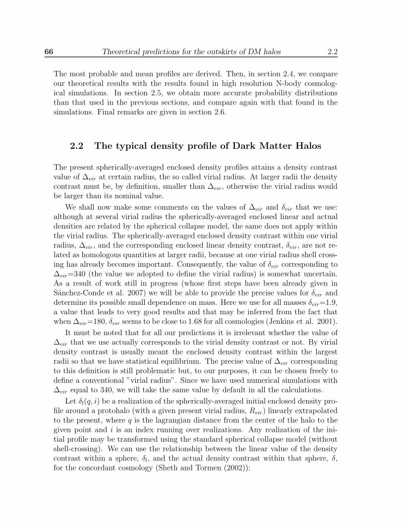
66 Theoretical predictions for the outskirts of DM halos 2.2
The most probable and mean profiles are derived. Then, in section 2.4, we compareour theoretical results with the results found in high resolution N-body cosmolog-ical simulations. In section 2.5, we obtain more accurate probability distributionsthan that used in the previous sections, and compare again with that found in thesimulations. Final remarks are given in section 2.6.
2.2 The typical density profile of Dark Matter Halos
The present spherically-averaged enclosed density profiles attains a density contrastvalue of ∆vir at certain radius, the so called virial radius. At larger radii the densitycontrast must be, by definition, smaller than ∆vir, otherwise the virial radius wouldbe larger than its nominal value.
We shall now make some comments on the values of ∆vir and δvir that we use:although at several virial radius the spherically-averaged enclosed linear and actualdensities are related by the spherical collapse model, the same does not apply withinthe virial radius. The spherically-averaged enclosed density contrast within one virialradius, ∆vir, and the corresponding enclosed linear density contrast, δvir, are not re-lated as homologous quantities at larger radii, because at one virial radius shell cross-ing has already becomes important. Consequently, the value of δvir corresponding to∆vir=340 (the value we adopted to define the virial radius) is somewhat uncertain.As a result of work still in progress (whose first steps have been already given inSanchez-Conde et al. 2007) we will be able to provide the precise values for δvir anddetermine its possible small dependence on mass. Here we use for all masses δvir=1.9,a value that leads to very good results and that may be inferred from the fact thatwhen ∆vir=180, δvir seems to be close to 1.68 for all cosmologies (Jenkins et al. 2001).
It must be noted that for all our predictions it is irrelevant whether the value of∆vir that we use actually corresponds to the virial density contrast or not. By virialdensity contrast is usually meant the enclosed density contrast within the largestradii so that we have statistical equilibrium. The precise value of ∆vir correspondingto this definition is still problematic but, to our purposes, it can be chosen freely todefine a conventional ”virial radius”. Since we have used numerical simulations with∆vir equal to 340, we will take the same value by default in all the calculations.
Let δl(q, i) be a realization of the spherically-averaged initial enclosed density pro-file around a protohalo (with a given present virial radius, Rvir) linearly extrapolatedto the present, where q is the lagrangian distance from the center of the halo to thegiven point and i is an index running over realizations. Any realization of the ini-tial profile may be transformed using the standard spherical collapse model (withoutshell-crossing). We can use the relationship between the linear value of the densitycontrast within a sphere, δl, and the actual density contrast within that sphere, δ,for the concordant cosmology (Sheth and Tormen (2002)):

2.2 The typical density profile of Dark Matter Halos 67
δl(δ) =1.676
1.68647
[
1.68647 − 1.35
(1 + δ)2/3− 1.12431
(1 + δ)1/2+
0.78785
(1 + δ)0.58661
]
(2.2)
or, rather its inverse function δ(δl) (Patiri et al.(2006) expression (4)):
δ(δl) = 0.993[(1 − 0.607(δl − 6.5 × 10⁻³(1 − θ(δl)+
+θ(δl − 1.55))δ2l ))−1.66 − 1] (2.3)
being θ the step function:
θ(x) =
1 if x > 00 if x ≤ 0
Transforming for every shell δl and q into δ and r (the Eulerian radius of theshell) we may obtain, in parametric form, the initial profile δl(q, i) spherically evolved,δ(r, i).
δ(r, i) = δ(δl(q, i)); r = [1 + δ(δl(q, i))]−1/3q (2.4)
Consider now the ensemble of all halos, δ(r, j), attaining a δ value equal to ∆vir ata virial radius and smaller values for larger radii. If we transform back these profile totheir linear counterpart, we obtain the ensemble δl(q, j). Let us now take the averageover this ensemble (now for a fixed value of q):
δ(q) ≡< δ(q, j) >j
Evolving this profile by means of the spherical collapse model we obtain a profilewhich we call typical profile and represent by δt(r), that is, this profile is simply themean profile in the initial conditions spherically evolved.
To obtain the mean linear density profile δl(q), in our approach we first obtainthe probability for δl(q) only with the condition δl(Q) = δvir:
P (δl, q) ≡ P (δl(q)|δl(Q) = δvir) =
exp
(
−12
(
δl(q)−σ12σ21
δvir
)2
g
)
√2π g
12
(2.5)
where
g(q) ≡(
σ22 −
σ212(q)
σ21
)
σ1 ≡ σ(Q); σ2 ≡ σ(q)
(σ(x))2 =1
2π2
∫ ∞
0
| δk |2 W 2T (xk) k2 dk
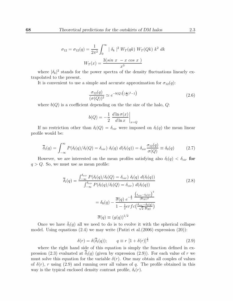
68 Theoretical predictions for the outskirts of DM halos 2.3
σ12 = σ12(q) =1
2π2
∫ ∞
0
| δk |2 WT (qk) WT (Qk) k2 dk
WT (x) =3(sin x − x cos x )
x3
where |δk|2 stands for the power spectra of the density fluctuations linearly ex-trapolated to the present.
It is convenient to use a simple and accurate approximation for σ12(q):
σ12(q)
(σ(Q))2≃ e−b(Q)
(
)2−1)
(2.6)
where b(Q) is a coefficient depending on the the size of the halo, Q:
b(Q) = −1
2
d ln σ(x)
d lnx
∣
∣
∣
∣
x=Q
If no restriction other than δl(Q) = δvir were imposed on δl(q) the mean linearprofile would be:
δl(q) =
∫ ∞
−∞P (δl(q)/δl(Q) = δvir) δl(q) d(δl(q)) = δvir
σ12(q)
σ(Q)≡ δ0(q) (2.7)
However, we are interested on the mean profiles satisfying also δl(q) < δvir forq > Q. So, we must use as mean profile:
δl(q) =
∫ δvir
−∞ P (δl(q)/δl(Q) = δvir) δl(q) d(δl(q))∫ δvir
−∞ P (δl(q)/δl(Q) = δvir) d(δl(q))(2.8)
= δ0(q) − σ(q) e− 1
2
(
δvir−δ0(q)
)2
(σ(q))2
1 − 12erfc
( δvir−δ0(q)√2 σ(q)
)
σ(q) ≡ (g(q))1/2
Once we have δl(q) all we need to do is to evolve it with the spherical collapsemodel. Using equations (2.4) we may write (Patiri et al.(2006) expression (20)):
δ(r) = δ(δl(q)); q ≡ r [1 + δ(r)]13 (2.9)
where the right hand side of this equation is simply the function defined in ex-pression (2.3) evaluated at δl(q) (given by expression (2.9)). For each value of r wemust solve this equation for the variable δ(r). One may obtain all couples of valuesof δ(r), r using (2.9) and running over all values of q. The profile obtained in thisway is the typical enclosed density contrast profile, δt(r).
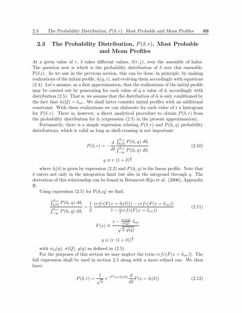
2.3 The Probability Distribution, P (δ, r). Most Probable and Mean Profiles 69
2.3 The Probability Distribution, P (δ, r). Most Probable
and Mean Profiles
At a given value of r, δ takes different values, δ(r, j), over the assemble of halos.The question now is which is the probability distribution of δ over this ensemble,P(δ,r). As we saw in the previous section, this can be done, in principle, by makingrealizations of the initial profile, δl(q, i), and evolving them accordingly with equations(2.4). Let’s assume, as a first approximation, that the realizations of the initial profilemay be carried out by generating for each value of q a value of δl accordingly withdistribution (2.5). That is, we assume that the distribution of δl is only conditioned bythe fact that δl(Q) = δvir. We shall latter consider initial profiles with an additionalconstraint. With these realizations we can elaborate for each value of r a histogramfor P (δ, r). There is, however, a direct analytical procedure to obtain P (δ, r) fromthe probability distribution for δl (expression (2.5) in the present approximation).
Fortunately, there is a simple expression relating P (δ, r) and P (δl, q) probabilitydistributions, which is valid as long as shell-crossing is not important:
P (δ, r) = − d
dδ
∫ δvir
δl(δ)P (δl, q) dδl
∫ δvir
−∞ P (δl, q) dδl(2.10)
q ≡ r (1 + δ)13
where δl(δ) is given by expression (2.2) and P (δl, q) is the linear profile. Note thatδ enters not only in the integration limit but also in the integrand through q. Thederivation of this relationship can be found in Betancort-Rijo et al. (2006), AppendixB.
Using expression (2.5) for P(δl,q) we find:
∫ δvir
δl(δ)P (δl, q) dδl
∫ δvir
−∞ P (δl, q) dδl=
1
2
erfc(F (x = δl(δ))) − erfc(F (x = δvir))
1 − 12erfc(F (x = δvir))
(2.11)
F (x) ≡x− σ12(q)
σ(Q)δvir
√
2 g(q)
q ≡ (r (1 + δ))13
with σ12(q), σ(Q), g(q) as defined in (2.5).For the purposes of this section we may neglect the term erfc(F (x = δvir)). The
full expression shall be used in section 2.5 along with a more refined one. We thenhave:
P (δ, r) =1√πe−F 2(x=δl(δ))
d
dδF (x = δl(δ)) (2.12)

70 Theoretical predictions for the outskirts of DM halos 2.3
By construction, δ at r must be smaller than ∆vir and larger than certain value,δmin(r):
δmin(r) = 341 (Rvir/r)3 − 1 (2.13)
This minimum value corresponds to a situation where there is no matter in be-tween Rvir and r. So, for δ values outside the interval (δmin(r),∆vir), P (δ, r) is zero.
We may obtain an analytical expression for P(δ,r) using approximation (2.6) forσ12(q)
σ21
and the following approximation for σ(q) (which enters g(q), defined below
expression (2.5)):
σ(q) ≃ (1.65 10−2 + 0.105(q h Mpc−1))−12 for q < 3 h−1Mpc
Expression (2.10) is valid as long as shell-crossing is not important. In Pradaet al. (2006) we have found by mean of comparison with numerical simulationsthat, beyond three virial radius, the relevance of shell-crossing diminishes quickly.This relevance can be estimated a priori (i.e. without comparison with simulations)obtaining P(δ,r) directly through realizations of the initial profile accordingly withexpression (2.5) and evolving them accordingly with equations (2.4). If shell-crossingwere irrelevant, the P(δ,r) obtained in this way should be equal to that given byexpression (2.12). The presence of certain amount of shell-crossing will cause theP(δ,r) obtained with realization to have a somewhat smaller maxima and a moreextended tail than that given by (2.12) (note that it is this expression that correspondsto realizations elaborated with expression (2.5). In this case none of the proceduresgives the correct P(δ,r) because both assume that δ is related to δl by means ofexpression (2.2), which is inconsistent when shell-crossing is important. However, thedifference between the results obtained with both procedures is of the same order ofthe difference between any of them and the profile obtained with a proper treatmentof shell-crossing. Note that even this last P(δ,r) is not the real one, since, as wesaid before, we are generating the initial profile using only a two point distribution(expression (2.5)).
In Figure 2.1 we compare the P(δ,r) obtained by the two procedures mentionedabove for several values of r expressed in unit of the virial radius (that we denote by s).We also show the corresponding histograms obtained from the numerical simulationsdescribed in Prada et al. (2006), which were done using the Adaptive RefinementTree (ART) code (Kravtsov et al. 1997) for the standard ΛCDM cosmological modelwith Ω0 = 0.3, ΩΛ = 0.7, h = 0.7, and cover a wide range of scales with different massand force resolutions (see Prada et al. 2006 for a detailed description). In particular,the histograms in Figure 2.1 were obtained for a total of 654 halos in a mass rangeof 3 ± 1 · 1012h−1 M⊙ selected without any kind of isolation criteria.
We can see that, for s = 2.5, where shell-crossing is already important, there issubstantial difference between the results of both procedures. A considerable amountof probability is transfered from the most probable value to much larger values (δ ≈

2.3 The Probability Distribution, P (δ, r). Most Probable and Mean Profiles 71
100) causing the distribution obtained through the realizations to be bimodal. Fors = 3.5 there is still a small amount of shell-crossing causing the maxima obtainedwith both procedures to differ by roughly a 20%. For larger values of s this differencesteadily diminishes.
Figure 2.1 P (δ, r) as given by expression (2.12) compared with the corresponding histogramobtained through realizations (histogram with small error bars) and that found in thesimulations (histogram with large error bars) for four values of s (≡ r/Rvir) and a mass of3 × 1012h−1 M⊙ (∆vir = 340 and δvir = 1.9).
Furthermore, as s increases the difference between the distribution given by ex-pression (2.12) and the histogram obtained with the numerical simulations reduces.In fact, even for s = 3.5 the relative values of P(δ,r) at different values of δ to the leftof the maxima are very well given by (2.12). The difference in the absolute valueswith respect to those in the histogram is due to the normalization. For δ values tothe right of the maxima, expression (2.12) gives a considerably more extended tailthan in the actual distribution. Therefore the normalization constant is larger in thelatter case.
Note that, although the maxima of expression (2.12) and that of the histogramcorresponding to the numerical simulations approach as s increases, due to the in-creasing irrelevance of the tail, this tail is still substantially more extended even for
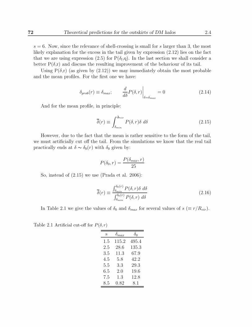
72 Theoretical predictions for the outskirts of DM halos 2.4
s = 6. Now, since the relevance of shell-crossing is small for s larger than 3, the mostlikely explanation for the excess in the tail given by expression (2.12) lies on the factthat we are using expression (2.5) for P(δl,q). In the last section we shall consider abetter P(δ,r) and discuss the resulting improvement of the behaviour of its tail.
Using P(δ,r) (as given by (2.12)) we may immediately obtain the most probableand the mean profiles. For the first one we have:
δprob(r) ≡ δmax;d
dδP (δ, r)
∣
∣
∣
∣
δ=δmax
= 0 (2.14)
And for the mean profile, in principle:
δ(r) ≡∫ ∆vir
δmin
P (δ, r)δ dδ (2.15)
However, due to the fact that the mean is rather sensitive to the form of the tail,we must artificially cut off the tail. From the simulations we know that the real tailpractically ends at δ ∼ δ0(r) with δ0 given by:
P (δ0, r) =P (δmax, r)
25
So, instead of (2.15) we use (Prada et al. 2006):
δ(r) ≡∫ δ0(r)
δminP (δ, r)δ dδ
∫ δ0(r)
δminP (δ, r) dδ
(2.16)
In Table 2.1 we give the values of δ0 and δmax for several values of s (≡ r/Rvir).
Table 2.1 Artificial cut-off for P (δ, r)
s δmax δ0
1.5 115.2 495.42.5 28.6 135.33.5 11.3 67.94.5 5.8 42.25.5 3.3 29.36.5 2.0 19.67.5 1.3 12.88.5 0.82 8.1

2.4 Comparison with N-body simulations 73
2.4 Comparison with N-body simulations
In this section we combine the statistics of the initial density fluctuations with thespherical collapse model to obtain predictions for the mean and most probable densityprofiles of collapsed galaxy-size dark matter halos with masses 1011−5×10¹²M⊙. Wethen compare our results with those obtained by means of high resolution N-bodycosmological simulations presented in Prada et al. (2006) for same halo masses andradii. The model gives excellent results beyond 2-3 formal virial radii.
In Figure 2.2 we have computed, both for δ and for δ′, the most probable (squares)and mean (crosses) density profiles found in our simulations for two mass intervalswith the mean values equal to the masses used in the theoretical derivation. We havetaken 277 halos in the mass range (6.5±1.5)×1010h−1 M⊙ and 654 halos in the massrange (3±1)×1012h−1 M⊙ (from Box80S and Box80G simulations, with parametersgiven in Table 2 of Prada et al. 2006). No isolation criteria was used. In Table 2.4we list for the mean halo with mass < M >= 3× 10¹²h−1 M⊙ the estimations of themost probable and mean value of the density at different radii compare with thatfrom the spherical collapse model for the most probable, the mean and the typicalprofiles.
In Figure 2.2 one can see that beyond 2 virial radius the mean and the mostprobable profiles, both for δ and for δ′, differ considerably. This is due to the factthat for this radii the probability distribution for δ, P (δ, r), is rather wide, witha long upper tail. This can be seen in Figure 2.3 were this distribution is showninside 3.5 ± 0.05 virial radius for the mass < M >= 3 × 10¹²h−1 M⊙. We show forcomparison the theoretical prediction for P (δ, r) as well as we give the most probableδmax and mean value < δ > of the distribution.
It is apparent from Figure 2.2 that the δ′ profiles are steeper for smaller masses, sothat they go below the background at smaller r/Rvir and reach larger underdensities.The δ profiles are also steeper for smaller masses although the difference is, obviously,much smaller. We have found that the theoretical prediction for the typical andthe most probable profile are, in general, almost indistinguishable (see Table 2.4).They are both found to be in very good agreement with the most probable δ profilefound in the numerical simulations beyond two virial radii. There is also qualitativeagreement between the predictions of the most probable δ′ profiles and those foundin the numerical simulations. It must be noted, however, that by predicted δ′ profilewe understand simply the one obtained from the corresponding δ profile by means ofrelationship given in Eq.(2.1). Note that this is not the same as the most probableprofile for δ′ (see Figure 2.2). This is due to the fact that the most probable δ′ valueat a given s(≡ r/Rvir) corresponds to a different halo than the most probable δ valueat the same s. This explains that, while the prediction for δprob agrees very well withthe simulations, the agreement is not so good for δ′prob. The δ′prob obtained from δprob
by means of expression Eq.(2.1) is not a proper prediction but an indicative value,since we can not envisage a feasible procedure to obtain a proper prediction. On

74 Theoretical predictions for the outskirts of DM halos 2.4
the contrary, the mean profiles < δ > are exactly related to < δ′ > by means ofexpression Eq.(2.1). The predictions for both profiles are in good agreement withthe numerical simulations, showing a much flatter profile beyond 2 virial radius thanthose corresponding to δprob and δ′prob. This agreement is remarkable given the factthat the expression used for P (δ, r) is only a first approximation (see next section).
Table 2.2 Comparison between the simulated mean halo density profile and the theoreticalpredictions from the spherical collapse model for the mass < M >= 3 × 10¹²h−1 M⊙.
Numerical Simulations Spherical Collapser/Rvir < δ > δprob < δ′ > δ′prob < δ > δprob δt < δ′ > δ′prob δ′t
1.0 337 323 69.1 52.4 531 398 385 40.4 2.5 7.81.5 129 116 30.8 15.1 184 115 118 22.6 1.9 4.32.0 67.7 54.6 19.5 3.73 84.8 53.7 51.7 14.7 1.5 2.82.5 43.2 31.1 15.4 1.6 49.3 28.6 27.6 10.3 1.2 1.93.0 30.8 17.4 11.2 0.78 32.2 17.3 16.6 7.6 1.0 1.43.5 22.1 12.6 8.5 0.58 22.6 11.3 10.9 5.8 0.79 0.974.0 18.4 9.0 5.9 0.18 16.8 7.9 7.6 4.5 0.61 0.704.5 14.1 5.8 5.5 0.09 13.0 5.8 5.5 3.5 0.46 0.505.0 12.2 4.4 4.3 -0.08 10.4 4.3 4.1 2.7 0.32 0.345.5 9.4 3.5 3.3 -0.16 8.5 3.3 3.2 2.1 0.20 0.226.0 7.9 2.8 3.1 -0.17 7.1 2.5 2.5 1.6 0.09 0.126.5 6.8 2.1 2.5 -0.22 5.7 2.0 2.0 1.2 -0.008 0.037.0 6.2 1.6 1.9 -0.33 4.6 1.6 1.6 0.9 -0.10 -0.04
Note. — The symbols < δ >, δprob, δt stand, respectively, for mean, most probable, and typ-ical averaged enclosed fractional overdensity. The corresponding primed simbols are for the localfractional overdensities at given radius.
It is interesting to note, as we have previously pointed out, that larger masseshave somewhat shallower profiles. In order to predict this trend correctly we mustuse the initial profile given by Eq.(2.9). If we dropped the second constraint used toderive this Eq.(2.9) and use in Eq.(2.9) the initial profile given by Eq.(2.7), whichcorresponds to high mass objects, the prediction would be the opposite. The reasonfor this being that, in this limit, the initial profile depend on mass only through c(the concentration parameter, defined as c ≡ Rvir/rs, where rs is a characteristicscale radius) which increases with increasing mass, thereby leading to steeper profiles
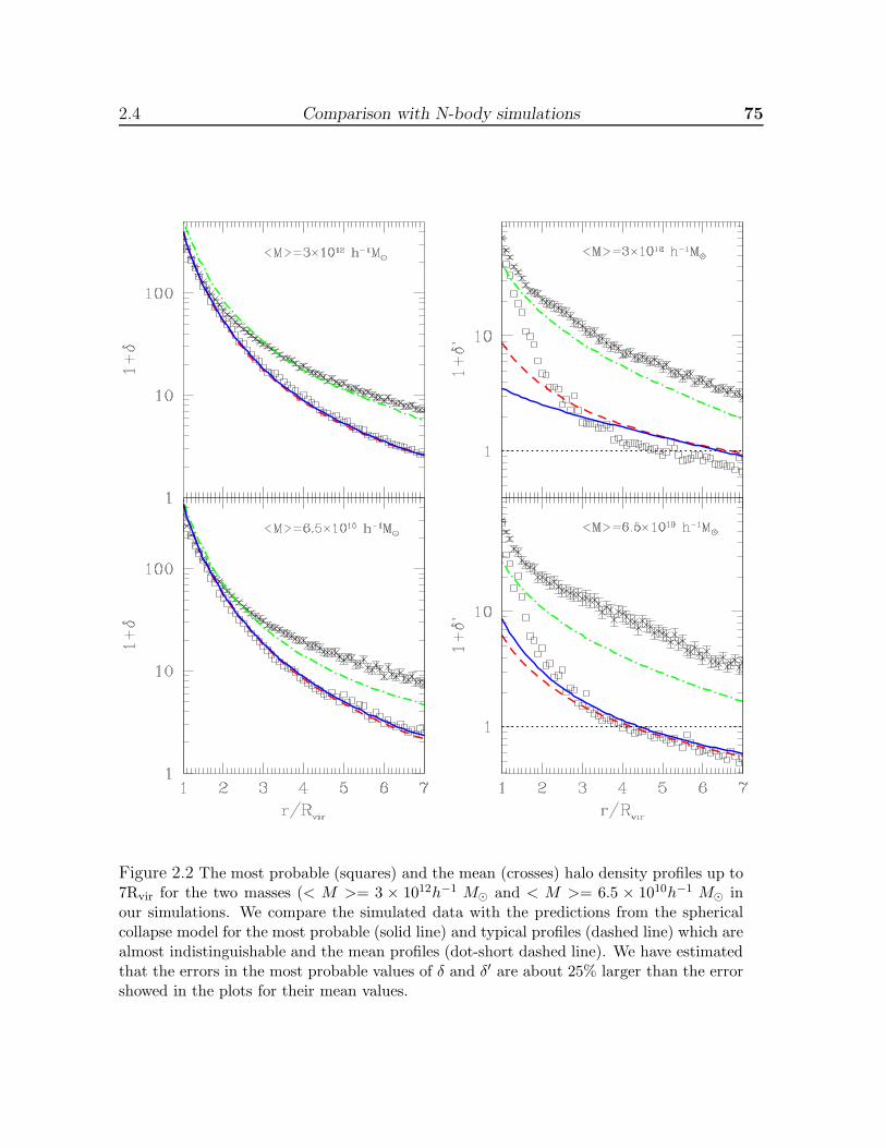
2.4 Comparison with N-body simulations 75
Figure 2.2 The most probable (squares) and the mean (crosses) halo density profiles up to7Rvir for the two masses (< M >= 3 × 10¹²h−1 M⊙ and < M >= 6.5 × 10¹⁰h−1 M⊙ inour simulations. We compare the simulated data with the predictions from the sphericalcollapse model for the most probable (solid line) and typical profiles (dashed line) which arealmost indistinguishable and the mean profiles (dot-short dashed line). We have estimatedthat the errors in the most probable values of δ and δ′ are about 25% larger than the errorshowed in the plots for their mean values.
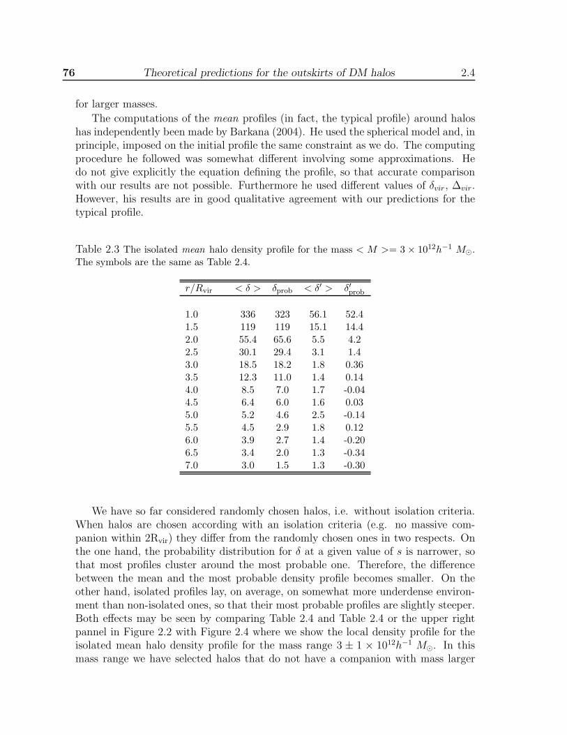
76 Theoretical predictions for the outskirts of DM halos 2.4
for larger masses.
The computations of the mean profiles (in fact, the typical profile) around haloshas independently been made by Barkana (2004). He used the spherical model and, inprinciple, imposed on the initial profile the same constraint as we do. The computingprocedure he followed was somewhat different involving some approximations. Hedo not give explicitly the equation defining the profile, so that accurate comparisonwith our results are not possible. Furthermore he used different values of δvir, ∆vir.However, his results are in good qualitative agreement with our predictions for thetypical profile.
Table 2.3 The isolated mean halo density profile for the mass < M >= 3 × 10¹²h−1 M⊙.The symbols are the same as Table 2.4.
r/Rvir < δ > δprob < δ′ > δ′prob
1.0 336 323 56.1 52.41.5 119 119 15.1 14.42.0 55.4 65.6 5.5 4.22.5 30.1 29.4 3.1 1.43.0 18.5 18.2 1.8 0.363.5 12.3 11.0 1.4 0.144.0 8.5 7.0 1.7 -0.044.5 6.4 6.0 1.6 0.035.0 5.2 4.6 2.5 -0.145.5 4.5 2.9 1.8 0.126.0 3.9 2.7 1.4 -0.206.5 3.4 2.0 1.3 -0.347.0 3.0 1.5 1.3 -0.30
We have so far considered randomly chosen halos, i.e. without isolation criteria.When halos are chosen according with an isolation criteria (e.g. no massive com-panion within 2Rvir) they differ from the randomly chosen ones in two respects. Onthe one hand, the probability distribution for δ at a given value of s is narrower, sothat most profiles cluster around the most probable one. Therefore, the differencebetween the mean and the most probable density profile becomes smaller. On theother hand, isolated profiles lay, on average, on somewhat more underdense environ-ment than non-isolated ones, so that their most probable profiles are slightly steeper.Both effects may be seen by comparing Table 2.4 and Table 2.4 or the upper rightpannel in Figure 2.2 with Figure 2.4 where we show the local density profile for theisolated mean halo density profile for the mass range 3 ± 1 × 10¹²h−1 M⊙. In thismass range we have selected halos that do not have a companion with mass larger
2.4 Comparison with N-body simulations 77
Figure 2.3 Distribution of the fractional cumulative density δ inside 3.5 ± 0.05Rvir for themean halo of mass < M >= 3 × 10¹²h−1 M⊙. We show for comparison the theoreticalprediction of P (δ, s) as well as we give the most probable δmax and mean value < δ > of thedistribution. We display the density distribution from its minimum value up to 1σ from itsmean < δ > (8% of the values of the distribution are beyond 1σ).
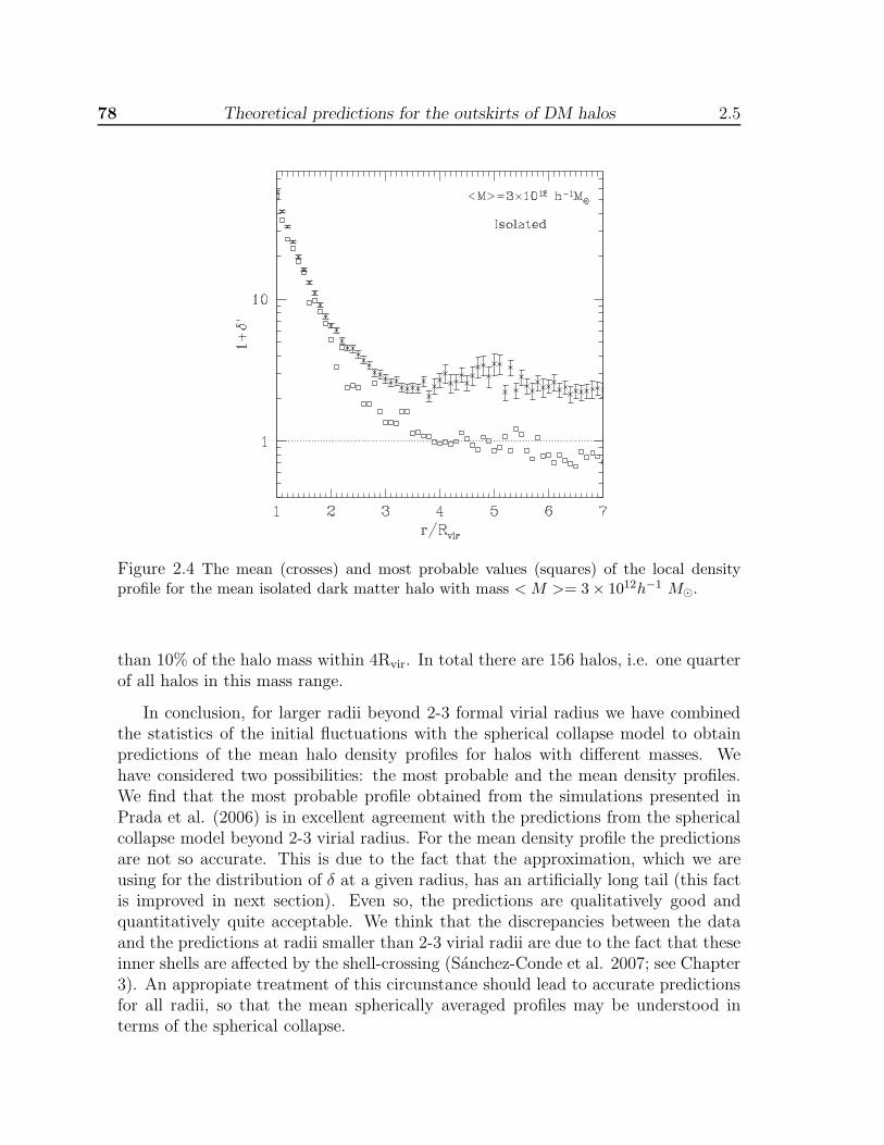
78 Theoretical predictions for the outskirts of DM halos 2.5
Figure 2.4 The mean (crosses) and most probable values (squares) of the local densityprofile for the mean isolated dark matter halo with mass < M >= 3 × 10¹²h−1 M⊙.
than 10% of the halo mass within 4Rvir. In total there are 156 halos, i.e. one quarterof all halos in this mass range.
In conclusion, for larger radii beyond 2-3 formal virial radius we have combinedthe statistics of the initial fluctuations with the spherical collapse model to obtainpredictions of the mean halo density profiles for halos with different masses. Wehave considered two possibilities: the most probable and the mean density profiles.We find that the most probable profile obtained from the simulations presented inPrada et al. (2006) is in excellent agreement with the predictions from the sphericalcollapse model beyond 2-3 virial radius. For the mean density profile the predictionsare not so accurate. This is due to the fact that the approximation, which we areusing for the distribution of δ at a given radius, has an artificially long tail (this factis improved in next section). Even so, the predictions are qualitatively good andquantitatively quite acceptable. We think that the discrepancies between the dataand the predictions at radii smaller than 2-3 virial radii are due to the fact that theseinner shells are affected by the shell-crossing (Sanchez-Conde et al. 2007; see Chapter3). An appropiate treatment of this circunstance should lead to accurate predictionsfor all radii, so that the mean spherically averaged profiles may be understood interms of the spherical collapse.

2.5 Improving P (δ, r) 79
2.5 Improving P (δ, r)
We have seen that for s (= r/Rvir) larger than 3 the realization of initial profilesand their subsequent evolution lead to values of P (δ, r) very close to those obtainedusing expression (2.12). This means that shell crossing is not important at theseradii. So, the difference between the actual value of P (δ, r) (the histogram obtainedfrom the simulations) and that given by expression (2.12) lies on the fact that thisexpression is only an approximation, or in the possible relevance of triaxiality, non-radial motions and pressure (velocity dispersions). To determine the amount of thediscrepancy due to inaccuracies in the statistical description of the initial conditionsas opposed to the discrepancy due to neglected dynamical factors, we must considerbetter approximation than that provided by expression (2.12). We shall use nowtwo improved approximations. The first one is that obtained by using expression(2.11) in expression (2.10), which we represent by P1(δ, r). Note that, to derive thisapproximation we have used the fact that at a given q larger thanQ, δl must be smallerthan δvir, but we have used expression (2.5) for P (δl, q). This distribution does notaccount for the fact that for all values of q larger than Q, δl < δvir. Consequently,P (δl, q) falls off with δl more slowly than it should and the same applies to P (δ, r). Inthe second approximation, which we represent by P2(δ, r), we consider a P (δl, q) whichtakes into account this additional constraint. By comparing the predictions obtainedwith P2(δ, r), P1(δ, r) with those obtained with P (δ, r) (expression (2.12)) we maycheck whether P1(δ, r) is accurate enough, so that the remaining discrepancy of theprediction with the results shown in the simulations may be ascribed to unaccounteddynamical factors.
To obtain P2(δl, q) we must first obtain the joint probability distribution for thevalue of δl at Q, q and at the middle point q′ = 1
2(q+Q). We represent by x1, x2, x3
respectively the value of δl at these three points.
The joint distribution for these three variables is a Gaussian trivariate distributionP (x1, x2, x3), which can be obtained for a given power spectra. With this distributionwe may immediately obtain the distribution of x3 conditioned to x1 = δvir, x2 < δvir,namely: P2(δl, q). So, we have:
P2(δl, q) =
∫ δvir
−∞ P (x2|x1) P (x3|x1, x2) dx2∫ δvir
−∞ P (x2|x1) dx2
(2.17)
where P (δvir, x2) is the joint probability distribution for x1, x2 with x1 = δvir.P2(δl, q) is the probability distribution of δl at q conditioned to δl(Q) = δvir andδl(q
′) < δvir. We have not imposed yet the almost redundant condition (since P2(δl, q)is very small for δl > δvir) that δl at q must be smaller than δvir. The probabilitydistribution for δl with this condition, P2(δl, q), is simply obtained through normal-ization. Here we have just discussed the main lines of the derivation of P2(δl, q). Afull description can be found in Betancort-Rijo et al. (2006).
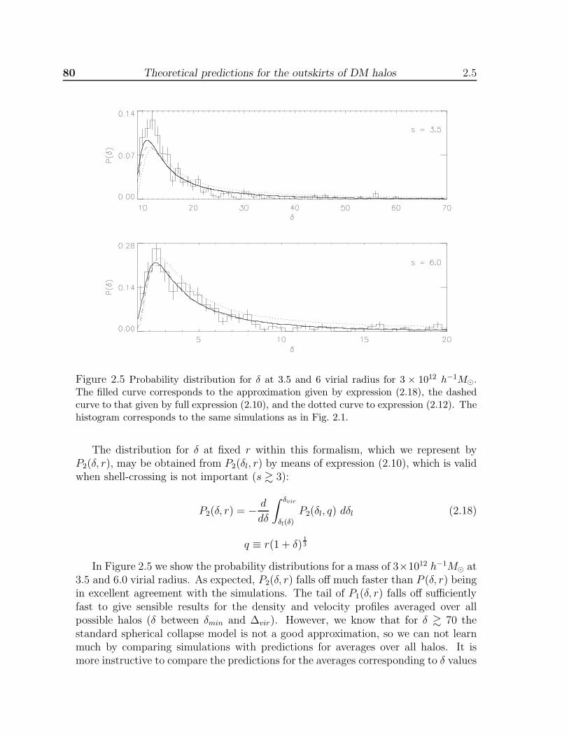
80 Theoretical predictions for the outskirts of DM halos 2.5
Figure 2.5 Probability distribution for δ at 3.5 and 6 virial radius for 3 × 10¹² h−1M⊙.The filled curve corresponds to the approximation given by expression (2.18), the dashedcurve to that given by full expression (2.10), and the dotted curve to expression (2.12). Thehistogram corresponds to the same simulations as in Fig. 2.1.
The distribution for δ at fixed r within this formalism, which we represent byP2(δ, r), may be obtained from P2(δl, r) by means of expression (2.10), which is validwhen shell-crossing is not important (s & 3):
P2(δ, r) = − d
dδ
∫ δvir
δl(δ)
P2(δl, q) dδl (2.18)
q ≡ r(1 + δ)13
In Figure 2.5 we show the probability distributions for a mass of 3×10¹² h−1M⊙ at3.5 and 6.0 virial radius. As expected, P2(δ, r) falls off much faster than P (δ, r) beingin excellent agreement with the simulations. The tail of P1(δ, r) falls off sufficientlyfast to give sensible results for the density and velocity profiles averaged over allpossible halos (δ between δmin and ∆vir). However, we know that for δ & 70 thestandard spherical collapse model is not a good approximation, so we can not learnmuch by comparing simulations with predictions for averages over all halos. It ismore instructive to compare the predictions for the averages corresponding to δ values

2.5 Improving P (δ, r) 81
Figure 2.6 Mean δ profile for 3 × 10¹² h−1M⊙ using the probability distribution given byexpression (2.12) (dashed line), by full expression (2.10) (3dots-dashed line) and by expres-sion (2.18) (dot-dashed line). Mean δ obtained from simulations is given for comparison(filled line). In all the cases, a maximum value of δ = 70 was used.
Figure 2.7 Mean δ profile for 3 × 10¹² h−1M⊙ using the probability distribution given byexpression (2.12) (dashed line), by full expression (2.10) (3dots-dashed line) and by expres-sion (2.18) (dot-dashed line). Mean δ obtained from simulations is given for comparison(filled line). For all radius, the average was calculated excluding the 20% of the halos withthe largest δ values.
between δmin (expression (2.13)) and 70 with those found in the simulations for thesame range of δ values.
In Figure 2.6 we show the predictions given by P (δ, r), P1(δ, r), P2(δ, r) for the
82 Theoretical predictions for the outskirts of DM halos 2.6
δ profile averaged between δmin and 70 and the averaged found in the simulations.Only the relevance of triaxiality can explain the results shown in Figure 2.6. Theeffect is not large in this Figure, since only a small fraction of the halos are affected,but it is quite meaningful.
Knowing that for some halos the spherical collapse model can not be a goodapproximation, the relevant question now is to determine precisely how good is it formost halos. To this end, at each radial bin we search for the value, δ1(r), such thatthe upper cumulative probability, as given by P2(δ, r), is 0.2, and eliminate, both inthe simulations and in the predictions, halos with larger δ values at that bin. Bydoing so, we eliminate many halos which simply have flatter profiles than average,but are otherwise sufficiently spherical for the model to apply. But, we are sure ofhaving eliminated all halos with highly triaxial outskirts, most of them correspondingto situations where a couple of halos lie within a few virial radius from each other, sothat each of them will show up in the outskirt of the other halo; a situation that, byno mean, can be described by the spherical model. The resulting profiles, as given bythe different approximations to P (δ, r) and the simulations are given in Figure 2.7.The difference between the various approximations is now smaller, since the maindifference occurs at the far tail (of P (δ, r)), which has now been eliminated, but thisdifference increases for smaller masses. The profile obtained from the simulations liesnow slightly below the best prediction, as it should be if the spherical model is a goodapproximation.
In summary, the distribution P2(δ, r) is very close to the exact. To most purposesthe simpler distribution P1(δ, r) may be used, their difference being small, althoughit increases for smaller values. The density profiles obtained with P2(δ, r) are in ex-cellent agreement with those found in simulations beyond ∼ 3 virial radius. Thedensity dispersion and the radial velocity show some discrepancy below ∼ 5 virial ra-dius, which clearly indicate the relevance of unaccounted dynamical factors, speciallyvelocity dispersions.
2.6 Final remarks
The spherical collapse model describes very well the properties of dark matter halosbeyond three virial radius. This could seem surprising given the fact that the densitycontours around halos may be considerably aspherical and the presence of tidal fields.
Nevertheless, the assumption that the spherically averaged density profiles atseveral virial radius evolves according with the spherical collapse model is not justa simplification introduced to make the problem tractable. The mean evolution isgiven by the spherical collapse model with some dispersion (for a given δl) due totriaxiality. This have been shown by mean of simulations (Lilje et al. 1986) andanalytical works (Bernardeau 1994). At sufficiently large radii where δ is sufficientlysmall (δ . 10) the fractional dispersion becomes small. At small radii, not only thedispersion becomes larger, causing the mean value of δ for a given δl to be somewhat

2.6 Final remarks 83
different from δ(δl) (expression (2.2)), but also the effect of non-radial motions andvelocity dispersions starts to dominate. So studying the dark matter profile wherethe uncertainty of the evolution is small, we may check that the initial conditionswe use are correct to a high degree of accuracy. With these conditions, as describedby the most accurate probability distribution, P2(δl, q), we should be able to obtainvery accurate predictions for all possible definitions (typical, mean...) of density andvelocity profile. Any residual discrepancy should be explained by triaxiality, non-radial motions and velocity dispersions, as we shall show in a future work, although,from the results shown in this work, the last two effects dominate at least up toroughly 5 virial radius. Going a step further, if we adequately take into account theneglected dynamical factors, the same initial conditions should explain the profile atany radii. In this way, we could be able to explain the dark matter profiles at leastdown to a virial radii understanding the role played by the initial conditions and bythe different processes relevant to the evolution.
Bibliography
Avila-Reese, V., Firmani, C. & Hernandez, X. 1998, ApJ, 505, 37
Ascasibar, Y., Yepes, G., Gottloeber, S. & Mueller, V. 2004, MNRAS, 352, 1109
Bajtlik S., Duncan R. C., Ostriker J. P., 1988, ApJ, 327, 570
Bardeen, J. M., Bond, J. R., Kaiser, N. & Szalay, A. S. 1986, ApJ, 304, 15 (BBKS)
Barkana R., 2004, MNRAS, 347, 59
Bernardeau, F. 1994, ApJ, 427, 51
Bertschinger, E. 1985, ApJS, 58,39
Betancort-Rijo J., Sanchez-Conde M. A., Prada F. & Patiri, S., 2006, ApJ, 649, 579
Brainerd, T.G., 2004, astro-ph/0409381
Conroy, C., Newman, J. A., Davis, M., Coil, A. L., Yan, R., Cooper, M. C., Gerke,B. F., Faber, S. M., & Koo, D. C., 2004, ApJ, 635, 982
Fillmore, J. A. & Goldreich, P. 1984, ApJ, 281, 1
Gunn, J. E. & Gott, J. R. 1972, ApJ, 176, 1
Gunn J. E., 1977, ApJ, 218, 592
Gurevich, A. V. & Zybin, K. P. 1988, ZHETF, 94, 3
Guzik, J., & Seljak, U., 2002, MNRAS, 335, 311
Hoekstra, H., Yee, H. K. C., Gladders, M. D., 2004, ApJ, 606, 67
Hiotelis, N. 2002, a, 382, 84
Hoffman Y., Shaham J., 1985, ApJ, 297, 16

2.6 BIBLIOGRAPHY 85
Jenkins A., Frenk C. S., White S. D. M., Colberg J. M., Cole S., Evrard A. E.,Couchman H. M. P., Yoshida N., 2001, MNRAS, 321, 372
Kravtsov, A.V., Klypin, A.A., & Khokhlov, A.M., 1997, ApJS, 111, 73
Lilje, P.B., Yahil, A. & Jones, B.J.T. 1986, ApJ, 307, L91
Lokas E. L., 2000, MNRAS, 311, 423
Lokas, E. L. & Hoffman, Y. 2000, ApJ, 542, L139
Nusser, A. 2001, MNRAS, 325, 1397
Padmanabhan T., 1996, MNRAS, 278, L29
Patiri S., Betancort-Rijo J. E. & Prada F. 2006, MNRAS, 368, 1132
Prada, F., Vitvitska, M., Klypin, A., Holtzman, J. A., Schlegel, D. J., Grebel, E. K.,Rix, H.-W., Brinkmann, J., McKay, T. A., & Csabai, I., 2003, ApJ, 598, 260
Prada F., Klypin A. A., Simmoneau E., Betancort-Rijo J., Patiri S. G., GottloberS., Sanchez-Conde M. A., 2006, ApJ, 645, 1001
Ryden, B. S. & Gunn, J. E. 1987, ApJ, 318, 15
Sanchez-Conde M. A., Betancort-Rijo J.E. and Prada F., 2007, MNRAS, 378, 339
Sheldon, E. S., et al., 2004, AJ, 127, 2544
Sheth, R. K. & Tormen, G. 2002, MNRAS, 329, 61
Sikivie, P., Tkachev, I. I. & Wang Y. 1997, Phys. Rev. D, 56(4), 1863 .
Smith, D. R., Bernstein, G. M., Fischer, P., & Jarvis, M., 2001, ApJ, 551, 643
Subramanian K., Cen R., Ostriker J. P., 2000, ApJ, 538, 528
White, S. D. M. & Zaritsky, D. 1992, ApJ, 394, 1
Zaritsky, D. & White, S. D. M. 1994, ApJ, 435, 599
Zaritsky, D., Smith, R., Frenk, C., & White, S. D. M. 1997, ApJ, 478, 39

86 BIBLIOGRAPHY 2.6

3The spherical collapse model with
shell-crossing1
In this work, we study the formation and evolution of dark matter halos by means ofthe spherical infall model with shell-crossing. We present a framework to tackle thiseffect properly based on the numerical follow-up, with time, of that individual shellof matter that contains always the same fraction of mass with respect to the totalmass. In this first step, we do not include angular momentum, velocity dispersion ortriaxiality. Within this framework - named as the Spherical Shell Tracker (SST) -we investigate the dependence of the evolution of the halo with virial mass, with theadopted mass fraction of the shell, and for different cosmologies. We find that ourresults are very sensitive to a variation of the halo virial mass or the mass fraction ofthe shell that we consider. However, we obtain a negligible dependence on cosmology.Furthermore, we show that the effect of shell-crossing plays a crucial role in the waythat the halo reaches the stabilization in radius and the virial equilibrium. We findthat the values currently adopted in the literature for the actual density contrast atthe moment of virialization, δvir, may not be accurate enough. In this context, westress the problems related to the definition of a virial mass and a virial radius forthe halo. The question of whether the results found here may be obtained by trackingthe shells with an analytic approximation remains to be explored.
3.1 Introduction
In the hierarchical scenario for structure formation in the Universe, the small primor-dial density fluctuations grow due to non-linear gravitational evolution and finallybecome the first virialized structures (halos). In this picture, larger Cold Dark Mat-ter (CDM) halos will be formed by the accretion and merger of those first smaller
1M. A. Sanchez-Conde, J. Betancort-Rijo and F. Prada, 2007, MNRAS, 378, 339
88 The spherical collapse model with shell-crossing 3.1
halos, forming in this way massive structures, and so on. This scenario, that con-stitutes the actual paradigm of hierarchical structure formation, is able to explainin general terms the universe that we see today. Yet, we do not have a frameworkor theory capable of reproducing this picture accurately. In this context, N-bodycosmological simulations are a powerful tool to try to understand the formation andsubsequent evolution of CDM halos. They constitute a very important help to buildany theoretical model and their predictions explain many of different observations.
Basically, there are two analytical approaches that make the problem tractable,although some simplifications have to be made and, as it was said, comparison be-tween these analytical studies and simulations are crucial to make progress: thePress-Schechter formalism (Press & Schechter 1974), based on the role of mergers(Nusser & Sheth 1999; Manrique et al. 2003), and the spherical infall model (SIM )focused on the understanding of the collapse of individual objects. We must note thatin the Press & Schechter formalism, the SIM has also been widely used, but from astatistical point of view, to treat problems related to mass accretion histories, massfunction, etc. The SIM, first developed by Gunn & Gott (1972) and Gunn (1977),describes the collision-less collapse of a spherical perturbation in an expanding back-ground. In those two articles, they introduced for the first time the cosmologicalexpansion and the role of adiabatic invariance in the formation of individual objects.Fillmore & Goldreich (1984) and Bertschinger (1985) found analytical predictions forthe density profiles of collapsed objects seeded by scale-free primordial perturbationsin a flat universe. Hoffman & Shaham (1985) generalized these solutions to realisticinitial profiles in flat and open Friedmann models, and Baarden et al. (1986) (here-after BBKS) improved this work introducing the peak formalism. Later, some studieshave been done to include more realistic dynamics of the growth process of dark mat-ter halos (e.g. Padmanabhan 1996; Avila-Reese, Firmani & Hernandez 1998; Lokas2000; Subramanian, Cen & Ostriker 2000).
In parallel, a large amount of numerical work have been done. Quinn, Salmon &Zurek (1986) and Frenk et al. (1988) obtained isothermal density profiles (ρ ∝ r−2)of CDM haloes, and Dubinski & Carlberg (1991) and Crone, Evrard & Richstone(1994) basically reproduced the predictions of Hoffman & Shaham (1985) and foundsome evidence for no pure power-law density profiles. Later, it was stablished thatthe density profiles of CDM halos have an universal form (Navarro, Frenk & White(1996, 1997, hereafter NFW), with ρ ∝ r−1 in the inner regions and ρ ∝ r−3 in theoutskirts, although there is still controversy about the shape of the profile near thecenter and recently it has been found that the pfoiles flatten out close to ρ ∝ r−2
beyond ∼ 2 virial radius. Moore et al. (1998,1999), amongst others, find ρ ∝ r−1.5
in the very center and other authors (Jing & Suto 2000; Klypin et al. 2001; Ricotti2003) find an inner slope ranging from −1 to −1.5 depending on halo mass, mergerhistory and substructure. Concerning to the outskirts of dark matter halos, Prada etal. (2006) carried out a detailed study and concluded that a 3D Sersic three param-eter approximation provides excelent density fits up to ∼ 2 times the virial radius,
3.1 Introduction 89
although these profiles differ considerably from the NFW ones beyond 2 virial radius.
There are also plenty of works in the literature using the SIM to predict the den-sity profiles of dark matter halos mainly focused on explaining their central regions.Moreover, the SIM has been widely used to obtain some quantities specially relevantand directly related to crucial stages in the formation and evolution of CDM haloesfor different cosmologies, redshifts, etc. A particularly relevant quantity is the valueof the overdensity at the moment of virialization δvir (∆vir usually in the literature),where overdensity is defined here as a number of times the background density, andits linear counterpart δl,vir. The values of δl,vir and δvir were obtained introducingthe virial theorem into the SIM formalism. This has important implications in theway we define the virial radius (the radius that attains an overdensity δvir inside) ofdark matter halos in N-body cosmological simulations. δvir is conventionally chosento be near 180 for an Einstein-deSitter cosmology (e.g. Peebles 1980), or 340 for theΩΛ = 0.7 cosmology (e.g. Bryan & Norman 1998; Lokas & Hoffman 2000).
In the standard derivation of δl,vir and δvir, the typical way to proceed is to assumethat a shell of matter stabilizes at an epoch twice the time of turn-around (i.e. thetime predicted by the standard SIM to collapse into a point), and in average witha radius that is 1/2 the turn-around radius (e.g. Peebles 1980; Lacey & Cole 1994;Eke, Cole & Frenk 1996). This 1/2 factor (in the Einstein-deSitter cosmology; forother cosmologies we need to use the Lahav equation, Lahav et al. 1991) is calledthe collapse factor. However, the justification to introduce this collapse factor and tosuppose the time of virialization as twice the time of turn-around, is poor and lacka solid theoretical background. In contrast, in this work we will study the sphericalcollapse without supposing any collapse factor, only taking into account the shell-crossing as the dominant effect. The angular momentum and velocity dispersion mayalso play an important role. The question is that if these effects were included inthe model, would we obtain the same values for δvir and δl,vir that those found inthe most simplistic scenario described by the standard SIM ? This issue is one of theaims of the present work.
The main goal of this line of work is to develop a theoretical framework that helpus to understand the dynamical elements that determine the process of formation ofstructures (collapsed objects) using spherical simmetry to explain main properties ofdark matter halos. In this first work we will tackle these questions by means of a”cold” collapse, that is, without including the effects of the velocity dispersion andangular momentum. The point is to ascertain if the non-uniformity of the densityprofiles generated via shell-crossing is able to provide the radial motions necessary toproduce the virialization and stabilization in an appropiate time scale. In a futurework, we will include the angular momentum and velocity dispersion to go a stepfurther.

90 The spherical collapse model with shell-crossing 3.1
There are some issues that it is worth to mention and that make this work differ-ent from previous works that also included the shell-crossing in their formalism (e.g.Lokas & Hoffman 2000; Nusser 2001; Hiotelis 2002; Ascasibar et al. 2004). The way toproceed in these works is to handle the effect of shell-crossing by means of an adiabaticinvariant, once the standard SIM becomes incorrect for late stages of the evolution.This adiabatic invariant, also known as radial action, makes the problem analiticallytractable, and is based on the fact that the potential evolves in a time larger than theorbital period of the most inner shells. In contrast, we will study the shell-crossingeffect doing a follow-up of the radius that contains inside always the same fraction ofthe virial mass. This way to tackle the problem is only one of the possible options,but is essential, for example, in order to build and study the relationship betweenthe actual enclosed density contrast δ, defined as δ = ρ(<r)−<ρm>
<ρm>, with < ρm > the
mean matter density of the Universe, and the linear density contrast, δl, obtainedfrom the linear theory. Only Gehard Lemson did something similar, although usingN-body simulations and mainly focused on showing how accurate are the predictionsof the standard SIM compared to his simulations (Lemson 1995). Despite the factthat he showed that the SIM is a powerful tool to understand the evolution of halos,he never provided detailed quantites and relations for the actual and linear densitycontrasts. The function δl(δ) is very important to obtain the density profiles of darkmatter halos, as we discussed in previous works (Prada et al. 2006; Betancort-Rijoet al. 2006). Sheth & Tormen (2002) parametrized this function for the standardSIM. The framework presented here will allow us in the near future to provide alsoa simple parametrization for δl(δ), but taking into account the important effect ofshell-crossing, together with others relevant effects such as the angular momentumand velocity dispersion. This will lead us, for example, to obtain δl,vir and its corre-sponding δvir, to explain the shape of the dark matter density profiles or to shed lighton the mass functions. All of this without supposing any collapse factor, as pointedbefore, or other vague assumptions. Nevertheless, it will not be possible to obtainuseful applications by the moment, since in this first work we will include in ourstudy only the shell-crossing, which is the dominant effect. The full treatment willbe done and presented in an upcoming work. Here we will provide the first results ofour theoretical framework related to the role played by the shell-crossing.
This work is organized as follows. In Section 3.2 we briefly describe the SIM andexplain the formalism and units that we will use in the rest of the work. In Section 3.5we will study in detail the dependence of the way that the evolution occurs varyingsome parameters, in particular, the virial mass of the halo, the fraction of mass for agiven virial mass, and the cosmology. Section 3.6 will be specially dedicated to themoments of virialization and stabilization according to a given criterion, and theirdependence with the same parameters described above. We will also emphasize herethe difference between these two concepts. Finally, in Section 3.10, we address the
3.3 The Spherical Shell Tracker Framework 91
main results and ideas of the work, and point the lines for a future work.
3.2 The Spherical Shell Tracker Framework
In this section, we first describe the standard SIM and its equations, and then wepresent the formalism that we will use in the rest of the work, which will imply todescribe the density profile and define our own unities. This will allow us to handleeasily the equations involved. Later, the algorithm that we used to obtain the resultswill be described carefully step by step. All together will be known as the SphericalShell Tracker Framework (SST ). The main objetive of this section is to make easiera possible reproduction and implementation of the SST framework.
3.3 The formalism
In a flat Universe with ΩΛ = 0, the evolution of a homogeneous spherical (positive)density perturbation (the simplest way to tackle the problem of structure formation)with a mass M and radius R, is given by Newtonian dynamics (as shown by Tolman1934 and Bondi 1947), provided that R be much smaller than the Hubble radius:
d2R
dt2=
−G M
R2(3.1)
Integrating, since M is constant by definition, we obtain:
1
2
dR
dt2− G M
R= E (3.2)
where E determines whether the sphere expands forever (E > 0) or it finallycontracts (E < 0).
We can describe this spherical perturbation with a large number of mass particles,and even it is possible and more useful to imagine these particles as concentric shells(thanks to spherical simmetry) that do not cross each other, and each of them witha radius r(j, t), where j denotes the shell, which satisfies equation (3.1):
d2r(j, t)
dt2=
−G M(j, t)
r(j, t)2(3.3)
where M(j, t) is the enclosed mass for each shell j at time t:
M(j, t) = ρcrit
(
4π
3r(j, t)3
)
[1 + δ(r(j, t))] (3.4)
being ρcrit the critical density of the Universe, and δ(r) the actual density contrastwhithin r(j, t):

92 The spherical collapse model with shell-crossing 3.3
ρcrit =3 H2
8π G; δ(r) =
ρ(< r)− < ρm >
< ρm >(3.5)
with H the Hubble constant, and< ρm > the mean matter density of the Universe.As long as shell-crossing does not occurs, the actual density contrast is related
to the linear one (given by the linear theory, see e.g. Padmanabhan 1993) in theEinstein-deSitter cosmology by the formula (Sheth & Tormen 2002):
δl(δ) =
[
1.68647 − 1.35
(1 + δ)2/3− 1.12431
(1 + δ)1/2+
0.78785
(1 + δ)0.58661
]
(3.6)
The inverse function, δ(δl), is given by (Patiri et al. 2004):
δ(δl) = 0.993[
(1 − 0.607(δl − 6.5 × 10⁻³(1 − θ(δl)+
+θ(δl − 1.55))δ2l ))−1.66 − 1
]
(3.7)
being θ the step function:
θ(x) =
1 if x > 00 if x ≤ 0
It is possible to make some simplifications in the equations, choosing in an ap-propiate manner the value of some parameters. In particular, we choose:
time unit = initial timelength unit = initial radius of the protohalo, Ri
mass unit = [1 + δ(Ri)]
According to these units, and taking into account equations (3.4) and (3.5), andan Einstein-deSitter cosmology (where H = 2
3t−1), we have:
Hi =2
3; ρcrit,i =
3
4π; G =
2
9(3.8)
where i refers to the initial time.The Lagrangian radius q for each shell j (i.e. the comoving radius at t → 0) is
related to the Eulerian one r by:
q(j) = ri(j) [1 + δ(ri(j))]13 (3.9)
So, for the initial enclosed mass of a shell j, we now have simply (using eq.(3.4)):
M(j, ti) = M(j) = q(j)3 (3.10)
We must note that this enclosed mass of a shell j, M(j), is different from themass of each shell, Mshell(j):
Mshell(j) = M(j) −M(j − 1)
3.3 The formalism 93
M(j, t) =
n∑
i=1
Mshell(i) always than r(i) ≤ r(j) (3.11)
To obtain q(j) using Eq.(3.9) we need δi(ri(j)), that is, the actual density contrastat initial time, and to this end we need the linear profile at initial time, δi
l(q(j)). Inthis work we will use the linear profile presented in Prada et al. (2006) and Betancort-Rijo et al. (2006):
δ0 = δl,virσ12(q)
σ(Q)(3.12)
where δl,vir is the linear density contrast at the moment of virialization, q andQ are the Lagrangian radii related to r and Rvir respectively, that can be obtainedusing equation (3.9), and:
(σ(x))2 =1
2π2
∫ ∞
0
| δk |2 W 2T (xk) k2 dk
σ12 = σ12(q) =1
2π2
∫ ∞
0
| δk |2 WT (qk) WT (Qk) k2 dk
WT (x) =3(sin x − x cos x )
x3(3.13)
where |δk|2 stands for the power spectra of the density fluctuations linearly ex-trapolated to the present.
There is a good approximation for δ0:
δ0 = δl,vir exp
[
−b(
( q
Q
)2 − 1
)]
b(Q) = −1
2
d lnσ(x)
d lnx
∣
∣
∣
∣
x=Q
(3.14)
with b a constant depending on the mass. In Table 3.1 we present the values of band Q that we use for each mass. Moreover, it is necessary to assign a value to δl,vir
so we can use the density profile, although one of our final objetives is to obtain aprecise value for it. In this work we used a δl,vir = 1.9, a value which led to goodresults in previous works (Prada et al. 2006; Betancort-Rijo et al. 2006).
Essentially, the profile given in Eq.(3.12) and its approximation in Eq.(3.14) takesinto account only the restriction δl(Q) = δl,vir. In Hiotelis (2002) and Ascasibar etal. (2004), a very similar density profile was also used, but using the BBKS peakformalism to compute the initial conditions. In a future work we will use a moresophisticated density profile that includes also the restriction δl(q) < δl,vir for q > Q(see Betancort-Rijo et al. (2006) for a more detailed description), resulting in steeperactual density profiles for smaller masses (as confirmed by numerical simulations, see

94 The spherical collapse model with shell-crossing 3.3
Prada et al. 2006). This fact will probably change slightly the results. For a solce ofsimplicity we have preferred to use now a simple profile, although the major resultsof this work will not depend on the assumed profile.
Table 3.1 Values of b and Q neccesary to use the approximation for δ0 given by (3.14).
M (h−1 M⊙) Q (h−1Mpc) b
6.5 × 10¹⁰ 0.57 0.18895 × 10¹¹ 1.1252 0.22023 × 10¹² 2.0445 0.25442 × 10¹³ 3.848 0.3015 × 10¹⁴ 11.125 0.41
For the Einstein-deSitter cosmology, the δil(q(j)) profile can be obtained from
equation (3.12) simply rescaling by:
δil(q(j)) =
1
1 + ziδl(q(j)) (3.15)
where zi is the redshift at initial time. We can obtain δi(ri(j)) from δil(q(j))
using the function given in (3.7). Inserting this δ(δil(q(j))) in Eq.(3.9) we obtain the
Lagrangian radius for each shell j, q(j), and also using Eq.(3.10 its enclosed massM(j).
Once we have the expressions related to the initial conditions and we have pre-sented the density profile, we need the equations of evolution. If the shells do notcross each other, then there is an analytical solution for (3.2) (e.g. Martınez & Saar2002) that can be written in the parametric form:
r = rc(1 − cosη); t = tc(η − sinη) (3.16)
where:
rc =GM
c2; tc =
rc
c;
dt
dη=R
c(3.17)
Here c is the velocity of light and we did a change to a nondimensional variableη. This solution means that the shell expands until it reaches a maximum radius rta,the turn-around radius, at a given time tta, which is different for each shell, and afterthat point the shell starts to contract. We can integrate analitically equation (3.3)to study the evolution of the spherical density perturbation, at least until the turn-around, thanks to the fact that the enclosed mass of the shells do not change withtime. Nevertheless, after the turn-around, the recollapse begins and the shell-crossingalso starts, so we can not proceed in the same way. At that point, it is common touse a prescription based on an adiabatic invariant, to account for this secondary infalland shell-crossing (e.g. Lokas & Hoffman 2000; Nusser 2001; Hiotelis 2002; Ascasibar

3.4 The algorithm 95
et al. 2004). On the other hand, one can also integrate numerically the equation(3.3), computing at each time step the new radius, velocity and enclosed mass foreach shell. This is the method that we use in our work. Our purpose is to study andto include the shell-crossing in our treatment in a natural way, i.e. without makingany assumption about the collapse factor, the time at which virialization occurs, orany other simplification.
We first divide our spherical density perturbation in n equal spherical shells(equivalent to particles), all of them with the same thickness, and later we choosethe shell j that contain a given fraction of mass of the total protohalo. We do sofor every time step, from the start of the evolution to the end: we recompute thenew enclosed mass for each shell at each time step, and we always select that onethat contains the fraction of mass we are interested in (in that sense, n must be bigenough to choose with high precission and without problems at each step a shell thatcontains exactly the required fraction of mass; in our case, n = 3000 was enough).If we follow for a long time the shell related to this fraction of mass, at the end itsradius will be almost constant (although the corresponding physical shell will changewith time), that is, we will reach stabilization (see section 4). Lu et al. (2006) useda similar algorithm, but they divided the halo in equal mass shells, instead of shellswith the same thickness, as we do. Moreover, their motivations were different, mainlyfocused on explain the inner shape of the density profiles, and they did not carriedout a follow-up of any shell in particular.
3.4 The algorithm
We now describe the algorithm we used to compute the relevant quantities (radius,velocity and enclosed mass) for each shell at each time step.
First, we need to obtain the initial conditions :
1. We divide the protohalo in n equal shells to calculate our array of initial radii,ri(j), that contains the radius r for all the shells. Remember that, in our units,the radius of the total cloud is the unity; moreover, j increases decreasing theradius, so r(j = 1) = Ri (the radius of the whole halo), and r(j = 3000) is theradius of the deepest shell.
2. In a first approximation, we make q(j) = ri(j). This will allow us to computea second and better estimation for q(j) using in an appropiate way the relationgiven by equation (3.9), that is:
q(j) = ri(j)[1 + δ(δil(q(j)))]
13 (3.18)
where we introduce in the right side the q(j) as given by the first approximation.The function δ(δl) is given by eq.(3.7) and δi
l(q(j)) is given by (3.15).
96 The spherical collapse model with shell-crossing 3.4
3. Now, we will use the q(j) obtained in the last step as a new approximation tocompute again a better estimation for q(j), according to eq.(3.18).
4. Step (iii) must be repeated until there is no difference between the q(j) that weobtain after each iteration.
5. With ri(j) and the last and best estimations for the initial Lagrangian radii ofthe shells, q(j), we can calculate the initial enclosed mass array, M(j), usingequation (3.10), and the mass of each shell, Mshell(j), knowing that Mshell(j) =M(j) −M(j − 1). We will need Mshell(j) later to compute the enclosed massarray at each time step, since the mass of each shell will be always the same,although the order of the shells will be modified.
6. We also need the initial velocity for each shell, vi(j), as given by the SIM(Betancort-Rijo et al. 2006):
vi(j) = Hi ri(j)
[
1 − 1
3
1
1 + δ(δil(q(j)))
× 1dδl(δ)
dδ|δ=δ(δi
l(q(j)))
δil(q(j))
]
(3.19)
where δl(δ) and δ(δl) are given by Eq.(3.6) and Eq.(3.7), and δil(q(j)) is given
by Eq.(3.15). Hi is the Hubble constant at initial time, which in our units isHi = 2/3.
7. Now it is possible to select the shell that contains the fraction of mass that weare interested in. Our studies will be focused on the follow-up of this shell inparticular.
Once we have calculated the initial conditions, we now need to obtain theequations of evolution:
8. In our units, equation (3.3) can be written as:
d2r(j, t)
dt2= −2
9
M(j, t)
r(j, t)2(3.20)
so the equations of the evolution for r(j) and v(j) are:
r(j, t+ ∆t) = r(j, t) + v(j, t) ∆t (3.21)
v(j, t+ ∆t) = v(j, t) − 2
9
M(j, t) ∆t
r(j, t)2(3.22)

3.4 The algorithm 97
9. We also need to compute how the linear and actual density contrasts evolvewith time:
δl(j, t) = δil(q(j)) t
23 (3.23)
δ(j, t) =
[
[1 + δ(δil(q(j)))]
(
ri(j)
r(j)
)3]
t2 − 1 (3.24)
10. At each time step, we need to recalculate the new enclosed mass array, M(j),using the shell mass array Mshell(j), since the enclosed mass for a given shell jis equal to:
M(j, t) =n∑
i=1
Mshell(i) always than r(i) ≤ r(j) (3.25)
11. At this point, we can select again the shell that contains that fraction of masswe want to study, to see what happens with its radius, velocity, and linear andactual density contrasts.
12. For each step, we will have to repeat (ix) to (xii).
It is worth to mention, for possible reproductions of the results, that the begin-ning was set to an initial redshift zi = 15, to make sure that we are still wellinside the linear regime, i.e. the initial value of δl is small enough. Moreover,we used an optimized temporal step of 0.003 in our units, which is good enoughto give us robust results of δl and δ (we checked these values using well knownmoments of the evolution like the turn around, where there is no shell-crossingyet).
Furthermore, there is another important question that it is necessary to takeinto account to implement without problems the described algorithm. This isthe fact that we have not included yet the effect of the velocity dispersion andangular momentum. Therefore, we are in a totally radial (cold) collapse and wewill have problems in the very center of the halo if we simply integrate numer-ically the equations following this framework. When we compute, accordingto equations (3.21) and (3.22), the new radius and velocity of a shell whichis located very near to the center, we can obtain at the following time step anegative radius and a positive velocity, which means that actually this shell hascrossed through the center and now it goes from the inner regions of the haloto the outer ones. Nevertheless, it will be very hard that the total energy willbe conserved in this process due to numerical reasons. The distance that theshell covers in only one time step is comparable to its radius, which gives a con-siderable “leak” of energy. There are different ways to solve this problem; oneof them, the solution we chose, is to define a parameter m to measure properly
98 The spherical collapse model with shell-crossing 3.5
this effect and to help us to prevent this lost of energy. If we define for eachshell the parameter m as m = dr/r(j, t) (where dr = r(j, t + ∆t) − r(j, t) isthe distance that the shell has covered along this time step), then there is noproblem while m is small enough, but when m reaches a larger value, the wayto minimize the lost of energy in the process is to change the velocity for itsabsolute value, and keeping intact the value that we have for the radius. Doingso, we skip the very center and the loss of energy will be minimum. After manyattemps, we saw that a value of m = 0.02 leads to very good results.
In the ΛCDM cosmology, the formalism and the algorithm are the same, but wemust introduce some changes in the initial conditions and in the equations of theevolution the spherical to take into account the different cosmology with Λ 6= 0. Theequations, modified adequately, are presented in Appendix A.1.
3.5 The evolution of the halo: effect of shell-crossing
At the beginning of the evolution, we will not obtain any difference using our for-malism or using the standard SIM, because there is no shell-crossing yet. However,when this effect starts it is clear that this will become false. However, the expecteddeviation with respect to that given by the standard SIM may be different if oneuses different values for the virial mass of the halo, or study different fractions ofmass respect to this virial mass, or if we move to a different cosmology. To this end,that is, to quantify in detail how big are the dependences on these kind of factors,we carried out a study with varying the virial mass of the halo, Mvir, the fraction ofmass related to this virial mass, what we call Mfrac, and the cosmology through thevalue of ΩΛ.
To illustrate the way that shell-crossing occurs and affects to the evolution of thehalo, in Figure 3.1 we show the evolution with time of the radius related to differentMfrac for the particular case of an Einstein-deSitter cosmology and a virial mass ofMvir = 3×10¹²h−1 M⊙. It was been done in units of the turnaround radius and time(so we can compare between different Mfrac in the same scale). It is worth to mentionthat Lemson (1995) presented in the same way data from his simulations and he ob-tained essentially the same results as shown here for the evolution of individual shells.
Before the first shell-crossing happens, the behaviour of the radii of different Mfrac
is essentially the same. This first shell-crossing occurs just before twice the time ofturn-around (the time of virialization for the usual models), and what we can see isthat this first shell-crossing means the beginning of the stabilization in radius, whichfinally occurs some time after that (in next section, we will carry out a detailed studyof this process together with the virialization). The larger radius oscillations for eachcurve beyond ∼ 4 t/ta (see Figure 3.1) are only noise due to the growth of numerical
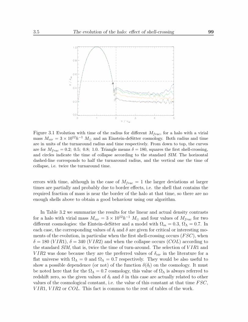
3.5 The evolution of the halo: effect of shell-crossing 99
Figure 3.1 Evolution with time of the radius for different Mfrac, for a halo with a virialmass Mvir = 3 × 10¹²h−1 M⊙ and an Einstein-deSitter cosmology. Both radius and timeare in units of the turnaround radius and time respectively. From down to top, the curvesare for Mfrac = 0.2; 0.5; 0.8; 1.0. Triangle means δ = 180, squares the first shell-crossing,and circles indicate the time of collapse according to the standard SIM. The horizontaldashed-line corresponds to half the turnaround radius, and the vertical one the time ofcollapse, i.e. twice the turnaround time.
errors with time, although in the case of Mfrac = 1 the larger deviations at largertimes are partially and probably due to border effects, i.e. the shell that contains therequired fraction of mass is near the border of the halo at that time, so there are noenough shells above to obtain a good behaviour using our algorithm.
In Table 3.2 we summarize the results for the linear and actual density contrastsfor a halo with virial mass Mvir = 3 × 10¹²h−1 M⊙ and four values of Mfrac for twodifferent cosmologies: the Eintein-deSitter and a model with Ωm = 0.3, ΩΛ = 0.7. Ineach case, the corresponding values of δl and δ are given for critical or interesting mo-ments of the evolution, in particular when the first shell-crossing occurs (FSC), whenδ = 180 (V IR1), δ = 340 (V IR2) and when the collapse occurs (COL) according tothe standard SIM, that is, twice the time of turn-around. The selection of V IR1 andV IR2 was done because they are the preferred values of δvir in the literature for aflat universe with ΩΛ = 0 and ΩΛ = 0.7 respectively. They would be also useful toshow a possible dependence (or not) of the function δ(δl) on the cosmology. It mustbe noted here that for the ΩΛ = 0.7 cosmology, this value of ΩΛ is always referred toredshift zero, so the given values of δl and δ in this case are actually related to othervalues of the cosmological constant, i.e. the value of this constant at that time FSC,V IR1, V IR2 or COL. This fact is common to the rest of tables of the work.

100 The spherical collapse model with shell-crossing 3.5
Table 3.2 Linear (δl) and actual (δ) density contrast values related to some importantmoments in the evolution of a halo with a virial mass Mvir = 3 × 10¹²h−1 M⊙ and for theEinstein-deSitter and Ωm = 0.3, ΩΛ = 0.7 cosmologies. See text for details.
Einstein-deSitter (Ωm = 1, ΩΛ = 0)
Mfrac = 0.2 Mfrac = 0.5 Mfrac = 0.8 Mfrac = 1.0Moment δl δ δl δ δl δ δl δ
FSC 1.667 1840 1.652 770 1.641 500 1.634 398VIR1 1.601 180 1.602 180 1.602 180 1.602 180VIR2 1.628 340 1.628 340 1.629 340 1.628 340COL 1.695 1426 1.695 653 1.696 424 1.696 350
Ωm = 0.3, ΩΛ = 0.7
Mfrac = 0.2 Mfrac = 0.5 Mfrac = 0.8 Mfrac = 1.0Moment δl δ δl δ δl δ δl δ
FSC 1.670 1728 1.655 761 1.644 516 1.639 427VIR1 1.608 180 1.606 180 1.605 180 1.605 180VIR2 1.632 340 1.632 340 1.631 340 1.631 340COL 1.698 1364 1.698 338 1.697 445 1.696 380
It is important to note here that, although Table 3.2 is only for a given virialmass, the same kind of study was done for the evolution of halos with virial massesMvir = 6.5 × 10¹⁰h−1 M⊙ and Mvir = 5 × 10¹⁴h−1 M⊙. We observed the same ten-dencies in the data and achieved the same conclusions. In Table 3.3 we show thevalues of δl and δ that we obtained for the three mentioned virial masses and for theEintein-deSitter and the Ωm = 0.3, ΩΛ = 0.7 cosmologies, for the particular case inwhich we fixed Mfrac=0.5.
Some interesting conclusions can be inferred from Figure 3.1 and Tables 3.2 and3.3. The most important ones can be summarized as follows:
1. FSC, the first shell-crossing, occurs earlier as Mfrac increases.
2. FSC occurs also earlier for larger masses.
3. FSC sets the beginning of the stabilization in radius.
4. FSC always occurs after V IR1 and V IR2 but always before COL, indepen-dently of Mvir and Mfrac.
5. V IR1 and V IR2 have essentially the same associated linear density contrasts,no matter the value of Mfrac or Mvir. This is because in all the cases, there
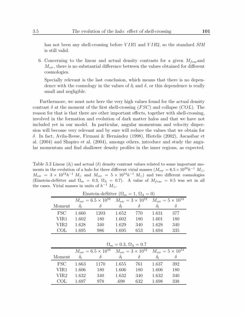
3.5 The evolution of the halo: effect of shell-crossing 101
has not been any shell-crossing before V IR1 and V IR2, so the standard SIMis still valid.
6. Concerning to the linear and actual density contrasts for a given MfracandMvir, there is no substantial difference between the values obtained for differentcosmologies.
Specially relevant is the last conclusion, which means that there is no depen-dence with the cosmology in the values of δl and δ, or this dependence is reallysmall and negligible.
Furthermore, we must note here the very high values found for the actual densitycontrast δ at the moment of the first shell-crossing (FSC) and collapse (COL). Thereason for that is that there are other important effects, together with shell-crossing,involved in the formation and evolution of dark matter halos and that we have notincluded yet in our model. In particular, angular momentum and velocity disper-sion will become very relevant and by sure will reduce the values that we obtain forδ. In fact, Avila-Reese, Firmani & Hernandez (1998), Hiotelis (2002), Ascasibar etal. (2004) and Shapiro et al. (2004), amongs others, introduce and study the angu-lar momentum and find shallower density profiles in the inner regions, as expected.
Table 3.3 Linear (δl) and actual (δ) density contrast values related to some important mo-ments in the evolution of a halo for three different virial masses (Mvir = 6.5×10¹⁰h−1 M⊙,Mvir = 3 × 10¹²h−1 M⊙ and Mvir = 5 × 10¹⁴h−1 M⊙) and two different cosmologies(Einstein-deSitter and Ωm = 0.3, ΩΛ = 0.7). A value of Mfrac = 0.5 was set in allthe cases. Virial masses in units of h−1 M⊙.
Einstein-deSitter (Ωm = 1, ΩΛ = 0)
Mvir = 6.5 × 10¹⁰ Mvir = 3 × 10¹² Mvir = 5 × 10¹⁴
Moment δl δ δl δ δl δ
FSC 1.660 1203 1.652 770 1.631 377VIR1 1.602 180 1.602 180 1.601 180VIR2 1.628 340 1.629 340 1.628 340COL 1.695 986 1.695 653 1.694 335
Ωm = 0.3, ΩΛ = 0.7
Mvir = 6.5 × 10¹⁰ Mvir = 3 × 10¹² Mvir = 5 × 10¹⁴
Moment δl δ δl δ δl δ
FSC 1.663 1170 1.655 761 1.637 392VIR1 1.606 180 1.606 180 1.606 180VIR2 1.632 340 1.632 340 1.632 340COL 1.697 978 .698 632 1.698 338

102 The spherical collapse model with shell-crossing 3.6
Hence, it will be absolutely necessary to take into account at least these two effectsif we want to go a step further in our analysis and if we want to obtain a good andaccurate parametrization for the function δl(δ). Nevertheless, the framework andalgorithm we are using, as well as the conclusions and tendences we can obtain onlyincluding the shell-crossing, are totally valid although we can not reach, by now, ex-act values. Including other effects in our framework, specially those ones mentionedabove, will be part of a future work.
Then, by the moment, we will not be able to provide an exact relation betweenthe linear and actual density contrasts, neither a parametric form for the functionδl(δ). However, we can have a look to the relation that we obtain at this momentbetween both density contrasts, and try to extract some conclusions. In Figure 3.2,the function δl(δ) is represented for the three virial masses under study and for theEinstein-deSitter cosmology. Figure 3.3 represents the same function but for differentcosmologies, in particular for the Einstein-deSitter case and Ωm = 0.3, ΩΛ = 0.7. Thelinear region is clearly visible in both figures below δl ∼ 1. In this regime there isno still any difference between the different curves and the value of δ grows veryslowly with δl, as expected. Then, there is a phase where δ increases very fast forsmall differences in δl, starting from δl ∼ 1.6 in all the cases. From this moment, thedependence with virial mass becomes clearly visible in figure 3.2, where we observethat the smaller the mass, the larger values of δ have reached for the same value of δl.Respect to the dependence on different cosmologies, it seems clear (see Figure 3.3)that this dependence is really small, as already mentioned.
Figure 3.2 The relation δl − δ for three virial masses. From down to top, the curves corre-spond to Mvir = 5 × 10¹⁴h−1 M⊙, Mvir = 3 × 10¹²h−1 M⊙ and Mvir = 6.5 × 10¹⁰h−1 M⊙(an Einstein-deSitter universe and Mfrac=0.5 was used in all the cases).
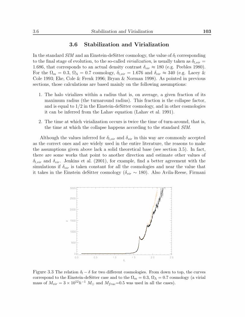
3.6 Stabilization and Virialization 103
3.6 Stabilization and Virialization
In the standard SIM and an Einstein-deSitter cosmology, the value of δl correspondingto the final stage of evolution, to the so-called virialization, is usually taken as δl,vir =1.686, that corresponds to an actual density contrast δvir ≈ 180 (e.g. Peebles 1980).For the Ωm = 0.3, ΩΛ = 0.7 cosmology, δl,vir = 1.676 and δvir ≈ 340 (e.g. Lacey &Cole 1993; Eke, Cole & Frenk 1996; Bryan & Norman 1998). As pointed in previoussections, those calculations are based mainly on the following assumptions:
1. The halo virializes within a radius that is, on average, a given fraction of itsmaximum radius (the turnaround radius). This fraction is the collapse factor,and is equal to 1/2 in the Einstein-deSitter cosmology, and in other cosmologiesit can be inferred from the Lahav equation (Lahav et al. 1991).
2. The time at which virialization occurs is twice the time of turn-around, that is,the time at which the collapse happens according to the standard SIM.
Although the values inferred for δl,vir and δvir in this way are commonly acceptedas the correct ones and are widely used in the entire literature, the reasons to makethe assumptions given above lack a solid theoretical base (see section 3.5). In fact,there are some works that point to another direction and estimate other values ofδl,vir and δvir. Jenkins et al. (2001), for example, find a better agreement with thesimulations if δvir is taken constant for all the cosmologies and near the value thatit takes in the Einstein deSitter cosmology (δvir ∼ 180). Also Avila-Reese, Firmani
Figure 3.3 The relation δl − δ for two different cosmologies. From down to top, the curvescorrespond to the Einstein-deSitter case and to the Ωm = 0.3, ΩΛ = 0.7 cosmology (a virialmass of Mvir = 3 × 10¹²h−1 M⊙ and Mfrac=0.5 was used in all the cases).

104 The spherical collapse model with shell-crossing 3.6
& Hernandez (1998) find that a diferent value of δl,vir respect to that deduced usingthe above assumptions makes better the comparison between the analytical Prech-Schechter mass distribution and the results of N-body simulations.
Moreover, there is another important question related to the virialization thatshould be considered here. In the framework of the standard SIM, it is possible toapply the virial theorem if we suppose the halo to be an isolated system. However,real halos are non-isolated systems, since they are immersed in large filamentarystructures, with surrounding material continously falling or scaping from the system,since they feel the tidal fields of their neighbours, etc. Hence, the virial theoremshould not be applied in this case. Despite of this fact, the standard SIM togetherwith the virial theorem have been used to obtain the values of δl,vir and δvir, and thesevalues have been taken as the references to define the virial radius and the virial massof the halos, which is specially adopted in N-body simulations. Furthermore, this facthas been traditionally supported for radial velocity early studies of massive dark mat-ter halos from simulations (Crone et al. 1994; Cole & Lacey 1996). These studiesapparently showed that the virial radius in this way defined (using δl,vir = 1.69 andδvir ∼ 180 in the Einstein-deSitter) constitutes an adequate boundary to separate theinner region of the halo in dynamical equilibrium, i.e. that region where the radialvelocities are zero, from the external region showing infall velocities. The popular-ization of these ideas came contemporarily with works that defined the virial massand virial radius in simulations according to these preliminary results (specially theNFW papers). But the fact is that, as recently shown in Prada et al. (2006), this maynot be totally correct. Concerning to galaxy-size halos, for example, they display allthe properties of relaxed objects up to ∼ 3 virial radius and there is no indicationof infall of material beyond. Therefore, there is no reason to believe that only insidethe virial radius, as currently defined, the halo is in equlibrium. In this context, it isimportant to understand the process of virialization more in depth.
In our work, no assumption is done related to the virialization. No collapse factor,no time for virialization a priori is adopted. Including shell-crossing in the way we dowill allow us to obtain δl,vir and its corresponding δvir in a natural way, i.e. studyingthe evolution of different shells of the halo according to the SST framework, presentedin section 2. It must be noted, however, that these values are still preliminary, since itwill be necessary to include the effects of angular momentum and velocity dispersionto obtain precise and useful values. Nevertheless, this study will be suitable to isolatethe role of shell-crossing and will be able to extract important conclusions related tothe stabilization and virialization. We believe that these conclusions will no changewhen we introduce other physical considerations into the framework.
It is important to note here the difference between these two concepts: stabiliza-tion and virialization. The first one can be inferred studying the behaviour of the
3.7 Stabilization 105
radius of a given shell that contains a given fraction of the virial mass with time, aswas shown in Figure 3.1. A criterion must be imposed to say if a given shell reachesstabilization or not, and when. The second concept, the virialization, will have to beinferred according to the virial theorem. There is no reason why stabilization andvirialization should coincide, although instinctively one expect that they should benear in time at least.
3.7 Stabilization
In first place, we define the time of stabilization as the time at which the radius ofthe shell that we are studying varies less than a given percent, and during -at least-an interval of time equal to once the time of turnaround. In practice, what we do isto choose the moment inmediately after the time of first shell-crossing, and we see ifthere is no a variation in radius larger than the maximum variation that we want toimpose as our criterion. It must be in this way during, at least, a time of turnaroundfrom this moment to forward. The value of reference that we take to measure thevariations in radius is the value of the radius at the initial moment of this interval. Ifthe percentage of variation of the radius is exceeded in any time within this interval,then we choose the moment inmediately after the previouly chosen, and so on untilwe find an interval of time where the criterion is satisfied. The first moment at whichthis occurs is our time of stabilization, and the value of the radius at the time ofstabilization is taken as our radius of stabilization.
This is illustrated in Figure 3.4, where the moments of stabilization are shown fora 5% and 10% of allowed variation of radius, for a particular cosmology (Ωm = 0.3,ΩΛ = 0.7), a value of Mfrac, and for different virial masses. As one can see, in thecase of 10% the stabilization is reached inmediately after the first shell-crossing, butthe stabilization according to only 5% of allowed variation of the radius is not reacheduntil roughly half of a time of turnaround later. Moreover, this stabilization remainsduring more than once the time of turnaround from that moment to forward (whichis the minimum required by our criterion). Only at late times, where the evolutionis dominated by numerical noise, the stabilization becomes worse than 5%. However,the most important conclusion is that the stabilization is not reached in any case fora radius that is 1/2 the radius of turnaround, value that corresponds to the collapsefactor assumed in the standard derivation of δl,vir and δvir. This fact constitutesanother proof that tell us how inappropiate are the current assumptions done aboutthe virialization.
A detailed study was done for different values of Mvir, Mfrac and cosmologies.A summary of this study can be found in Appendix A.2, Tables A.1 and A.2. Inthese tables we present the values for the density contrasts that we obtain for twodifferent degrees of stabilization (5% and 10%), with varying Mvir, Mfrac and for the

106 The spherical collapse model with shell-crossing 3.8
Figure 3.4 Stabilization at 5% (circles) and 10% (crosses) for the particular case of ΩΛ = 0.7and Mfrac = 0.5 for three different virial masses. From down to top, the curves correspondto Mvir = 6.5 × 10¹⁰h−1 M⊙ Mvir = 3 × 10¹²h−1 M⊙ Mvir = 5 × 10¹⁴h−1 M⊙. Again, thehorizontal dashed-line corresponds to half the turnaround radius, and the vertical one thetime of collapse, i.e. twice the turnaround time.
Einstein-deSitter and Ωm = 0.3, ΩΛ = 0.7 cosmologies.
3.8 Virialization
Concerning to the virialization, what we did was to calculate the kinetic and potentialenergies related to the shell that we want to study. Then, we estimate the degreeof agreement respect to that given by the virial theorem (i.e. U + 2K = 0, whereU and K are the potential and kinetic energies related to the shell under study) bymeans of the quantity |2K−U |/2K. It must be noted that, if the virial theorem wasexactly satisfied by the shell at some moment of its evolution, this quantity shouldbe at that time equal to zero.
The algoritm to define the moment and radius of virialization is the same as al-ready described for the stabilization. When we find an interval where the degree ofvirialization that we want to impose is satisfied in every moment inside this interval,then we define our time and radius of virialization as those ones corresponding tothe beginning of the interval considered. Again, as in the case of the stabilization, adetailed study was done for different values of Mvir, Mfrac and cosmologies. We sum-marize the results found in Tables A.3 and A.4 of Appendix A.2. In these tables wepresent the values for the density contrasts that we obtain for two different degrees ofvirialization (25% and 35%), with varying Mvir, Mfrac and for the Einstein-deSitter
3.9 Comparison between stabilization and virialization: general considerations 107
and Ωm = 0.3, ΩΛ = 0.7 cosmologies.
There is one issue related to Tables A.3 and A.4 that it is worth to mention. Inthose tables, a percent of 25% and 35% was set to look for virialization. This wasdone in this way because we noticed that below these percents it is impossible toreach virialization in most cases according to our criterion. A smaller percent meansa degree of virialization too strong to be satisfied. Nevertheless, it seems that, whenthe virialization is reached using these high percents, the halo has actually reachedthe virialization. This may be inferred from the fact that the individual percentsthat we measure in every moment within the interval considered does not decreasemonotonically from the beginning of the interval to its end. In fact, what one obtainsis a small fluctuation around (and near) the high percent that was imposed to find thevirialization. That is, the degree of virialization does not vary substantially withinthe whole interval, only small fluctuations are found. There is a possible explanationto the fact that we have actually reached virialization but the degree of virializationthat we find according to our definition is still above 20% or more. Until now, wehave used the standard virial theorem, that only involves the kinetic and potentialenergies. However, because of we are treating with a non-isolated system, with shellsof matter continously going in and going out from the system that we are consideringas our halo, we should include in the theorem another extra term. This term wouldbe related to the pressures involved in the system, and surely may be the explanationand the cause of this “residual” percent that we obtain in all the cases.
3.9 Comparison between stabilization and virialization:
general considerations
A summary of our results concerning to the degree of both stabilization and virializa-tion for a given shell can be found in Tables 3.4 and 3.5. In these tables, we show thedegree of stabilization and virialization reached for two known moments of evolution,V IR1 and V IR2 (see section 3), for different values of Mvir, Mfrac and cosmologies.It must be noted that the numbers given for the stabilization are calculated taking asreference the moment of evolution where we have stabilization in radius better than10%.
Both tables provide useful results to extract important conclusions. In first place,one can see that the points V IR1 and V IR2 are really far from the stabilizationand also from the virialization, although these points are the preferred values forthe moment of virialization in most of the works. In fact, in all the cases the firstshell-crossing occurs even after V IR1 and V IR2, as pointed in section 3.5, so itis not possible that the shell has reached virial equilibrium or simply stabilizationin radius at that moment. Also Lemson (1995) found similar results using N-body

108 The spherical collapse model with shell-crossing 3.9
Table 3.4 Degree of agreement with the virial theorem (VIR) and the moment of stabi-lization (STA) for two moments of evolution, VIR1 and VIR2, and for different values ofMfrac and two cosmologies. A virial mass of Mvir = 3 × 10¹² h−1 M⊙ was used in all thecases. See text for details.
Einstein-deSitter (Ωm = 1, ΩΛ = 0)
Mfrac = 0.2 Mfrac = 0.5 Mfrac = 0.8 Mfrac = 1.0Moment VIR STA VIR STA VIR STA VIR STA
VIR1 4.64 0.57 2.98 0.43 2.58 0.33 1.01 0.25VIR2 4.12 0.47 2.80 0.31 1.01 0.19 1.01 0.09
Ωm = 0.3, ΩΛ = 0.7
Mfrac = 0.2 Mfrac = 0.5 Mfrac = 0.8 Mfrac = 1.0Moment VIR STA VIR STA VIR STA VIR STA
VIR1 4.32 0.49 2.75 0.35 1.80 0.23 1.42 0.19VIR2 3.88 0.39 2.40 0.21 1.65 0.07 1.31 0.05
simulations, i.e. the equilibrium is reached in a longer time respect to that predictedby the standard SIM. This fact was one of the reasons to carry out the study inthe way already described in the subsections dedicated to the stabilization and thevirialization (with the results summarize in Tables A.1 to A.4). This alternative wayis based on looking for the moment where we really have reached stabilization andvirialization. In the first case according to a percent that we impose for the allowedvariation of the radius during a significative interval of time; in the second case forthe degree of agreement with the virial theorem during a similar interval. In mostof the cases, both stabilization and virialization were obtained far from the valueδl = 1.686 or δl = 1.676, the preferred values of δl,vir for the Einstein-deSitter andthe Ωm = 0.3, ΩΛ = 0.7 cosmology respectively.
Concerning to the associated values of the actual density contrast, δ, we find veryhigh values in most cases. It should be noted, however, that it is expected that thesevalues decrease substantially when we include angular momentum and velocity dis-persion in the formalism. So, the values showed in these tables are totally related tothe isolated effect of shell-crossing.
There are also other issues that could be interesting to stress, and that should beexplored more in detail in a future work:
1. Concerning to V IR1 and V IR2, the degree of both virialization and stabiliza-tion is better for longer values of Mvir.
2. Concerning to V IR1 and V IR2, the degree of both virialization and stabiliza-tion is also better for longer values of Mfrac.
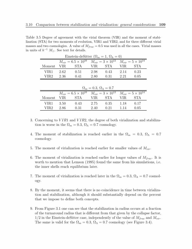
3.10 Comparison between stabilization and virialization: general considerations 109
Table 3.5 Degree of agreement with the virial theorem (VIR) and the moment of stabi-lization (STA) for two moments of evolution, VIR1 and VIR2, and for three different virialmasses and two cosmologies. A value of Mfrac = 0.5 was used in all the cases. Virial massesin units of h−1 M⊙. See text for details.
Einstein-deSitter (Ωm = 1, ΩΛ = 0)
Mvir = 6.5 × 10¹⁰ Mvir = 3 × 10¹² Mvir = 5 × 10¹⁴
Moment VIR STA VIR STA VIR STA
VIR1 2.62 0.51 2.98 0.43 2.14 0.23VIR2 2.36 0.41 2.80 0.31 2.21 0.05
Ωm = 0.3, ΩΛ = 0.7
Mvir = 6.5 × 10¹⁰ Mvir = 3 × 10¹² Mvir = 5 × 10¹⁴
Moment VIR STA VIR STA VIR STA
VIR1 3.50 0.43 2.75 0.35 1.18 0.17VIR2 2.86 0.31 2.40 0.21 1.14 0.05
3. Concerning to V IR1 and V IR2, the degree of both virialization and stabiliza-tion is worse in the Ωm = 0.3, ΩΛ = 0.7 cosmology.
4. The moment of stabilization is reached earlier in the Ωm = 0.3, ΩΛ = 0.7cosmology.
5. The moment of virialization is reached earlier for smaller values of Mvir.
6. The moment of virialization is reached earlier for longer values of Mfrac. It isworth to mention that Lemson (1995) found the same from his simulations, i.e.the inner shells reach equilibrium later.
7. The moment of virialization is reached later in the Ωm = 0.3, ΩΛ = 0.7 cosmol-ogy.
8. By the moment, it seems that there is no coincidence in time between virializa-tion and stabilization, although it should substantially depend on the percentthat we impose to define both concepts.
9. From Figure 3.1 one can see that the stabilization in radius occurs at a fractionof the turnaround radius that is different from that given by the collapse factor,1/2 in the Einstein-deSitter case, independently of the value of Mfrac and Mvir.The same is valid for the Ωm = 0.3, ΩΛ = 0.7 cosmology (see Figure 3.4).
110 The spherical collapse model with shell-crossing 3.10
3.10 Summary and future work
In this work we have studied the effect of shell-crossing in the formation and subse-quent evolution of dark matter halos. To do that, we have used the spherical collapsemodel, which has been widely used in the literature for more than thirty years tomanage and solve questions related to these processes. Nevertheless, despite of thelarge amount of works that have used this model or many others that have tried toimprove it by introducing in the formalism more and more complex considerations,any of them have included the effect of shell-crossing accurately. It is expected thatthis effect of shell-crossing will play a crucial role in the subsequent evolution of theobject. However, until now the shell-crossing has been always treated analytically,usually by means of an adiabatic invariant. This fact has paradoxically implied tomanage this effect in a very generic way, not capable to provide exact results andpredictions of relevant quantities or properties of dark matter halos.
Here we first use the exact expressions of the standard SIM, together with a re-alistic density profile, to compute the initial conditions. Then, we handle the effectof shell-crossing numerically. This allows us to study individually any shell of matterinvolved in the process of formation of the halo. Doing so, we can extract multipleconclusions about the way that this process occurs, like the relation between thelinear and actual density contrasts, the process of stabilization of a shell of matter,the virialization, etc. Most of these issues have been treated in the present work to agreater or lesser extent, although the main objetive have been always the developingof an adequate framework -the SST framework- in which we can study in depth theshell crossing and also other secondary effects.
It is possible to summarize the main conclusions of this work as follows:
1. The SST framework is adequate to tackle the effect of shell-crossing in a wayso we can extract exact results for different issues related to the evolutionof the halo: the way that the radius of a given shell evolves with time, therelation between the linear and actual density contrasts, the stabilization, thevirialization, etc.
2. The shell-crossing by itself is able to produce stabilization and virialization.Nevertheless, by the moment, it is not possible to obtain the exact values ofthe linear and actual density contrasts related to both moments of evolution.It is neccesary to take into account also other important effects.
3. Concerning to the relation between the linear and actual density contrasts, thedependence of this relation with the cosmology is very small and practicallynegligible. This conclusion is contrary to most of previous works, which find ingeneral a large dependence with cosmology. However, the dependence with thevirial mass or the fraction of virial mass that we consider, is large.
3.10 Summary and future work 111
4. Neither stabilization nor virialization are reached in a time according to thatgiven by the common assumptions related to the collapse factor and the time ofvirialization. In all the cases, we find that both stabilization and virializationoccur at larger times.
5. The values tipically used in the literature for δl,vir and δvir seem to be clearlyinadequate and incorrect, and are based on not very solid assumptions. In thiswork, new values of δl,vir and δvir are presented, but only taking into accountthe effect of shell-crossing. It will be neccesary to include in our frameworkother effects also relevant to be able to provide useful and final values for δl,vir
and δvir.
It is worth to emphasize that this work constitutes only a first step in our at-tempt to obtain exact and precise predictions related to the formation and evolutionof dark matter halos. In the future we plan to include in our framework other im-portant effects that it will be absolutely neccesary to take into account if we reallywant to provide more useful results. In particular, including the angular momentumand velocity dispersion will be the next. Furthermore, in parallel we will implementa more sophisticated density profile than that used in this work, which fixes betterthat found in the simulations and could change the results presented here slightly.One of the final aims of this future work will be to provide a simple parametrizationfor the relation δl − δ, which takes into account the effects of shell-crossing, angularmomentum and velocity dispersion, and include also the dependences observed withthe virial mass and the fraction of virial mass.
It is also in our mind to explore most of these questions using the cosmologicalN-body simulations together with theSST framework. Comparison between bothanalytical and simulation studies will be, by sure, crucial to reach a better and deeperunderstanding of the processes involved in the formation and evolution of dark matterhalos.
Bibliography
Avila-Reese, V., Firmani, C. & Hernandez, X. 1998, ApJ, 505, 37
Ascasibar, Y., Yepes, G., Gottloeber, S. & Mueller, V. 2004, MNRAS, 352, 1109
Bardeen, J. M., Bond, J. R., Kaiser, N. & Szalay, A. S. 1986, ApJ, 304, 15 (BBKS)
Barkana R., 2004, MNRAS, 347, 59
Bertschinger, E. 1985, ApJS, 58,39
Betancort-Rijo J., Sanchez-Conde M.A., Prada F., Patiri S.G., 2006, ApJ, in press,astro-ph/0509897
Bondi H., 1947, MNRAS, 107, 410
Bryan G., Norman M., 1998, ApJ, 495, 80
Cole S., Lacey C., 1996, MNRAS, 281, 716
Crone M.M., Evrard A.E., Richstone D.O., 1994, ApJ, 432, 402
Dubinski J., Carlsberg R.G., 1991, ApJ, 378, 496
Eke V.R., Cole S., Frenk C.S., 1996, MNRAS, 282, 263
Fillmore, J. A. & Goldreich, P. 1984, ApJ, 281, 1
Frenk C.S., White S.D.M., Davis M., Efstathiou G., 1988, ApJ, 327, 507
Gunn, J. E. & Gott, J. R. 1972, ApJ, 176, 1
Gunn J. E., 1977, ApJ, 218, 592
Hiotelis, N. 2002, a, 382, 84
Hoffman Y., Shaham J., 1985, ApJ, 297, 16
3.10 BIBLIOGRAPHY 113
Jenkins A., Frenk C. S., White S. D. M., Colberg J. M., Cole S., Evrard A. E.,Couchman H. M. P., Yoshida N., 2001, MNRAS, 321, 372
Jing Y.P., Suto Y., 2000, ApJ, 529, L69
Klypin A., Kravtsov A.V., Bullock J.S., Primack J.R., 2001, ApJ, 554, 903
Lacey C., Cole S., 1994, MNRAS, 271, 676
Lahav O., Lilje P.B., Primack J.R., Rees M.J., 1991, MNRAS, 251, 128
Lemson G., 1995, PhD: Statistics and dynamics of the perturbed universe, Gronin-gen University
Lokas E. L., 2000, MNRAS, 311, 423
Lokas, E. L. & Hoffman, Y. 2000, ApJ, 542, L139
Lu Y., Mo H.J., Katz N., Weinberg D., 2006, MNRAS, 368, 1931
Manrique A., Raig A., Salvador-Sole E., Sanchis T., Solanes J.M., 2003, ApJ, 593,26
Martınez V.J., Saar E., 2002, Statistics of galaxy distribution, Chapman &Hall/CRC
Moore B., Governato F., Quinn T., Stadel J., Lake G., 1998, ApJ, 499, L5
Moore B., Quinn T., Governato F., Stadel J., Lake G., 1999, MNRAS, 310, 1147
Navarro, J.F., Frenk C.S., White S.D.M., 1996, ApJ, 462, 563
Navarro, J.F., Frenk C.S., White S.D.M., 1997, ApJ, 490, 493
Nusser A., Sheth R.K., 1999, MNRAS, 303, 685
Nusser, A. 2001, MNRAS, 325, 1397
Padmanabhan T., 1993, Structure formation in the Universe, Cambridge UniversityPress, Cambridge
Padmanabhan T., 1996, MNRAS, 278, L29
Patiri S., Betancort-Rijo J. E. & Prada F., 2004, MNRAS, 368, 1132
Peebles P.J.E., 1980, The large-scale structure of the universe, Princeton UniversityPress, Princeton, N.J.

114 BIBLIOGRAPHY 3.10
Prada F., Klypin A. A., Simmoneau E., Betancort-Rijo J., Patiri S. G., GottloberS., Sanchez-Conde M. A., 2006 ApJ, 645, 1001
Press W.H., Schechter P., 1974, ApJ, 187, 425
Ricotti M., 2003, MNRAS, 344, 1237
Quinn P.J., Salmon J.K., Zurek W.H., 1986, Nat, 322, 329
Shapiro P.R., Illiev I.T., Martel H., Alvarez M.A., 2004, astro-ph/0409173
Sheth, R. K. & Tormen, G. 2002, MNRAS, 329, 61
Subramanian K., Cen R., Ostriker J. P., 2000, ApJ, 538, 528
Tolman R.C., 1934, Relativity, Thermodynamics, and Cosmology. Clarendon Press,Oxford

Part II
γ-ray Dark Matter searches:detection prospects

4Dark matter annihilation in Draco and
detection prospects1
A new revision of the gamma flux that we expect to detect in Imaging AtmosphericCherenkov Telescopes (IACTs) from neutralino annihilation in the Draco dSph ispresented in the context of the minimal supersymmetric standard models (MSSM)compatible with the present phenomenological and cosmological constraints, and usingthe dark matter (DM) density profiles compatible with the latest observations. Thisrevision takes also into account the important effect of the Point Spread Function(PSF) of the telescope, and is valid not only for Draco but also for any other DMtarget. We show that this effect is crucial in the way we will observe and interpret apossible signal detection. Finally, we discuss the prospects to detect a possible gammasignal from Draco for current or planned γ-ray experiments, i.e. MAGIC, Fermiand GAW. Even with the large astrophysical and particle physics uncertainties wefind that the chances to detect a neutralino annihilation signal in Draco seem to bevery scarce for current experiments. However, the prospects for future IACTs withupgraded performances (especially lower threshold energies and higher sensitivities)such as those offered by the CTA project, might be substantially better.
4.1 Introduction
Nowadays, it is generally believed that only a small fraction of the matter in theUniverse is luminous. In the Cold Dark Matter (CDM) cosmological scenario aroundone third of the “dark” side of the Universe is supposed to be composed of weakly in-teracting massive particles (WIMPs). although other possible candidates like axinosor gravitinos are not excluded (see Bertone et al. 2005 for a recent review). The Stan-dard Model can not provide a suitable explanation to the dark matter (DM) problem.
1M. A. Sanchez-Conde, F. Prada, E. L. Lokas, M. E. Gomez, R. Wojtak and M. Moles, 2007,Phys. Rev. D, 76, 123509

118 Dark matter annihilation in Draco and detection prospects 4.1
However, its supersymmetric extension (SUSY) provides a natural candidate for DMin the form of a stable uncharged Majorana fermion, called neutralino, which consti-tutes also one of the most suitable candidates according to the current cosmologicalconstraints. At present, large effort is being carried out to detect this SUSY DMby different methods (Munoz 2004). In the case of the new Imaging AtmosphericCherenkov Telescopes (IACTs), the searches are based on the detectability of gammarays coming from the annihilation of the SUSY DM particles. IACTs in operation likeMAGIC (Lorentz et al. 2004) or HESS (Hinton et al. 2004), or satellites-based exper-iments like the Fermi satellite (previously known as GLAST) (Gehrels & Michelson1999), will play a very important role in these DM searches.
A relevant question concerning the search of SUSY DM is where to search for theannihilation gamma ray signal. Due to the fact that the gamma flux is proportionalto the square of the DM density, we will need to point the telescope to places wherewe expect to find a high concentration of dark matter. In principle, the best optionseems to be the Galactic Centre (GC), since it satisfies this condition and it is alsovery near compared to other potential targets. However, the GC is a very crowdedregion, which makes it difficult to discriminate between a possible γ-ray signal due toneutralino annihilation and other astrophysical sources. Whipple (Kosack et al. 2004),Cangaroo (Tsuchiya et al. 2004), and specially HESS (Aharonian et al. 2004) andMAGIC (Albert et al. 2006) have already carried out detailed observations of the GCand all of them reported a gamma point-like source at the Sag A* location. However,if this signal was interpreted as fully due to DM annihilation, it would correspond toa very massive neutralino very difficult to fit within the WMAP cosmology (Spergelet al. 2007) in the preferred SUSY framework (Bergstrom et al. 2005), althoughan alternative scenario with multi-TeV neutralinos compatible with WMAP is stillpossible (see Profumo 2006). Furthermore, an extended emission was also discoveredin the GC area, but it correlates very well with already known dense molecular clouds(Aharonian et al. 2006). Recently, new HESS data on the GC have been published anda reanalysis has been carried out by the HESS collaboration (Aharonian et al. 2006b).In this work, they especially explore the possibility that some portion of the detectedsignal is due to neutralino annihilation. According to their results, at the momentit is not possible to exclude a DM component hidden under a non-DM power-lawspectrum due to an astrophysical source.
There are also other possible targets with high dark matter density in relativeproximity from us, e.g. the Andromeda galaxy, the dwarf spheroidal (dSph) galaxies- most of them satellites of the Milky Way- or even massive clusters of galaxies (e.g.Virgo). DSph galaxies represent a good option, since they are not plagued by theproblems of the GC, they are dark matter dominated systems with very high massto light ratios, and at least six of them are nearer than 100 kpc from the GC (Draco,LMC, SMC, CMa, UMi and Sagittarius).
Concerning DM detection, there are two unequivocal signatures that make surethat the γ-ray signal is due to neutralino annihilation: the spectrum of the source and
4.1 Introduction 119
its spatial extension. Certainly, the spectrum shape is crucial to state that the gammasource is due to DM annihilation, not only to discriminate it from the astrophysicalbackgrounds (e.g. hadronic, electronic and diffuse for IACTs), but also from any otherastrophysical sources. The keypoint here is that the spectrum of a DM annihilationsource is supposed to be in concordance with that expected from the models of particlephysics. Indeed, the exact annihilation spectra of MSSM neutralinos depend on thegaugino/higgsino mixing, but all of them show a continuum curved spectrum upto the mass of the DM particle and possibly faint γ-lines superimposed (Bergstrom2000). This spectrum will be very different from those measured in the case ofan astrophysical source (Aharonian et al. 2006b). As for the spatial extension ofthe source, in this case the important feature is that it should be extended anddiffuse, showing also a characteristic shape of the gamma flux profile. Nevertheless,we must note that if we use an instrument that does not have a spatial resolutiongood enough compared to the extension of the source, we might see only a point-likesource instead of a diffuse or extended one. This means that, although we mightreach high enough sensitivity for a successful detection, we would not be completelysure whether our signal is due to DM annihilation or not. Therefore, it is clear that itis really important to resolve the source so we can conclude that it can be interpretedas neutralino annihilation.
In this work, we first calculate the gamma ray flux profiles expected in a typicalIACT due to neutralino annihilation in the Draco dSph, which represents in principlea good candidate to search for DM. Draco, located at 80 kpc, is one of the dwarfs withmany observational constraints, which has helped to determine better its DM densityprofile. This fact is very important if we really want to make a realistic predictionof the expected γ-ray flux. These flux predictions have been already done for Dracousing different models for the DM density profiles (Bergstrom & Hooper 2006; Evanset al. 2004; Colafrancesco et al. 2007; Mambrini et al. 2006). Nevertheless, in ourcase, we compute these flux predictions for a cusp and a core DM density profilesbuilt from the latest stellar kinematic observations together with a rigorous method ofremoval of interloper stars. This computation represents by itself a recommendableupdate of the best DM model for Draco, but as we will see it will be also usefulto extract some important conclusions concerning the possible uncertainties in theabsolute γ-ray flux coming from astrophysics.
Once we have obtained the flux profiles, we will use them to stress the role of thePoint Spread Function (PSF) of the telescope. Including the PSF, which is directlyrelated to the angular resolution of the IACT, is essential to interpret correctly apossible signal profile due to neutralino annihilation, not only for Draco but also forany other target. In fact, we will show that, depending on the PSF of the IACT,we could distinguish or not between different models of the DM density profile usingthe observed flux profile. In the case of the cusp and core DM density profiles thatwe use, it could be impossible to discriminate between them if the PSF is not goodenough. It is worth mentioning that most of previous works in the literature (except
120 Dark matter annihilation in Draco and detection prospects 4.2
Prada et al. 2004) that calculated the expected flux profiles in IACTs due to darkmatter annihilation did not take into account this important effect. Because of that,to emphasize the role of the PSF constitutes also one of the goals of this work.
Finally, we present the DM detection prospects of Draco for some current orplanned experiments, i.e. MAGIC, Fermi and GAW. We carry out the calculationsunder two different approaches: detection of the gamma ray flux profile from the cuspand core DM models for Draco, and detection of an excess signal in the direction of thedwarf galaxy. We will show how the first approach could give us a lot of informationabout the origin of the gamma ray flux profile, but it is slightly harder to have successfor this case compared to the second approach, where even the PSF of the instrumentis not essential and still we could extract some important conclusions if we reachedthe required sensitivity.
The paper is organized as follows. In Section 4.2 we first present all the equationsnecessary to properly calculate the expected γ-ray flux in IACTs due to neutralinoannihilation. Both the particle physics and the astrophysics involved are describedcarefully. For the particle physics we analyze neutralino annihilation in the context ofthe minimal supersymmetric standard models (MSSM) compatible with the presentphenomenological and cosmological constraints. In Section 4.3 we show in detail themodel that we use for the DM distribution in Draco. In Section 4.4 we calculate theDraco flux predictions. We also stress the important role of the PSF. In Section 4.5,the prospects to detect signal due to neutralino annihilation in Draco are shown forsome current or planned experiments, i.e. MAGIC, Fermi and GAW. Conclusions arefinally given in Section 4.6.
4.2 The γ-ray flux in IACTs
The expected total number of continuum γ-ray photons received per unit time andper unit area in a telescope with an energy threshold Eth is given by the product oftwo factors:
F (E > Eth) =1
4πfSUSY · U(Ψ0). (4.1)
where Ψ0 represents the direction of observation relative to the centre of the darkmatter halo. The factor fSUSY includes all the particle physics, whereas the factorU(Ψ0) involves all the astrophysical properties (such as the dark matter distribu-tion and geometry considerations) and also accounts for the beam smearing of thetelescope.
4.2.1 Particle physics: the fSUSY parameter
In R-parity conserving supersymmetric theories, the lightest SUSY particle (LSP) re-mains stable. The widely studied Minimal Supersymmetric extension of the Standard
4.2 The γ-ray flux in IACTs 121
Model (MSSM) can predict a neutralino as the LSP with a relic density compatiblewith the WMAP bounds. In this section we concentrate on the MSSM under theassumption that the neutralino is the main component of the DM present in the uni-verse. We consider its abundance inside the bounds 0.09 < Ωχh
2 < 0.13 as derivedby fitting the ΛCDM model to the WMAP data (Spergel et al. 2007), although thepossibility for other DM candidates is not excluded (see Bertone 2005, Munoz 2004)and references therein).
The properties of the neutralinos in the MSSM are determined by its gaugino-higgsino composition:
χ ≡ χ01 = N11B +N12W
3 +N13H01 +N13H
02 (4.2)
At leading order, neutralinos do not annihilate into two-body final states containingphotons. However, at one loop it is possible to get processes such as (Bergstrom &Ullio 1997; Bern et al. 2007; Ullio & Bergstrom 1997):
χ + χ → γγ
χ + χ → Zγ
with monochromatic outgoing photos of energies
Eγ ∼ mχ, Eγ ∼ mχ − m2Z
4mχ
(4.3)
respectively. Also, the neutralino annihilation can produce a continuum γ – rayspectrum from hadronization and subsequent pion decay which can be dominate overthe monochromatic γ’s.
The lack of experimental evidence of supersymmetric particles leaves us with anumber of undetermined parameters in the SUSY models. Therefore, the annihilationcross sections involved in both the computation of Ωχh
2 and γ production can changeorders of magnitude with neutralino mass and its gaugino–higgsino composition. Tobe specific we consider mSUGRA models, where the soft terms of the MSSM aretaken to be universal at the gauge unification scale MGUT . Under this assumption,the effective theory at energies below MGUT depends on four parameters: the softscalar mass m0, the soft gaugino mass m1/2, the soft trilinear coupling A0, and theratio of the Higgs vacuum expectation values, tanβ = 〈H0
u〉 / 〈H0d〉. In addition, the
minimisation of the Higgs potential leaves undetermined the sign of the Higgs massparameter µ.
To provide some specific values, we assume A0 = 0, µ > 0 and two values of tan β,10 and 50. With this two cases we can provide a qualitative picture of most relevantspace of parameters and the constraints imposed by phenomenology. The impact ofthe size of A0 or the sign of µ can be found in several studies of the parameter spaceof the MSSM (see e.g. Cerdeno et al. 2003; Gomez et al. 2005; Gomez et al. 2003;Stark et al. 2005 and references therein).
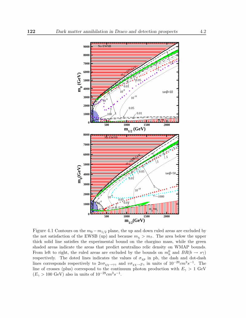
122 Dark matter annihilation in Draco and detection prospects 4.2
500 1000 1500 2000m1/2 (GeV)
0
1000
2000
3000
4000
5000
6000
7000
8000
9000
m0 (
GeV
)
No EWSB
0.05
0.01
0.01
0.05
5
5
mχ>mτ
m χ+=105 GeV
10-9
10-8
10-10
tanβ=10
100 1
500 1000 1500 2000m1/2(GeV)
0
1000
2000
3000
4000
5000
6000
7000
8000
m0(G
eV)
10-10
10-9
10-8
0.050.01
0.01
5
0.05
5m χ
+=105 GeV
mχ>mτ
No EWSB
tanβ=50
5
1000
Figure 4.1 Contours on the m0 −m1/2 plane, the up and down ruled areas are excluded bythe not satisfaction of the EWSB (up) and because mχ > mτ . The area below the upperthick solid line satisfies the experimental bound on the chargino mass, while the greenshaded areas indicate the areas that predict neutralino relic density on WMAP bounds.From left to right, the ruled areas are excluded by the bounds on m0
h and BR(b → sγ)respectively. The doted lines indicates the values of σχp in pb, the dash and dot-dashlines corresponds respectively to 2vσχχ→γγ and vσχχ→Zγ in units of 10−29cm3s−1. Theline of crosses (plus) correspond to the continuum photon production with Eγ > 1 GeV(Eγ > 100 GeV) also in units of 10−29cm3s−1.
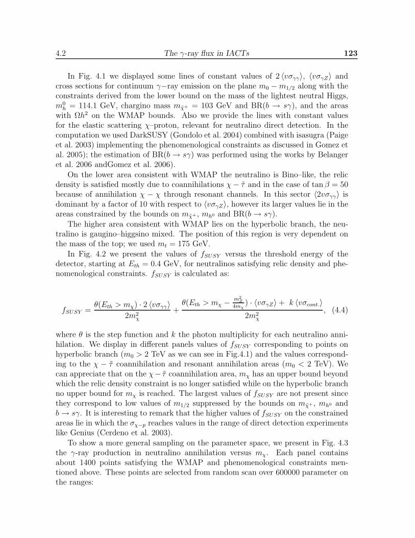
4.2 The γ-ray flux in IACTs 123
In Fig. 4.1 we displayed some lines of constant values of 2 〈vσγγ〉, 〈vσγZ〉 andcross sections for continuum γ−ray emission on the plane m0 −m1/2 along with theconstraints derived from the lower bound on the mass of the lightest neutral Higgs,m0
h = 114.1 GeV, chargino mass mχ+ = 103 GeV and BR(b → sγ), and the areaswith Ωh2 on the WMAP bounds. Also we provide the lines with constant valuesfor the elastic scattering χ–proton, relevant for neutralino direct detection. In thecomputation we used DarkSUSY (Gondolo et al. 2004) combined with isasugra (Paigeet al. 2003) implementing the phenomenological constraints as discussed in Gomez etal. 2005); the estimation of BR(b→ sγ) was performed using the works by Belangeret al. 2006 andGomez et al. 2006).
On the lower area consistent with WMAP the neutralino is Bino–like, the relicdensity is satisfied mostly due to coannihilations χ− τ and in the case of tanβ = 50because of annihilation χ − χ through resonant channels. In this sector 〈2vσγγ〉 isdominant by a factor of 10 with respect to 〈vσγZ〉, however its larger values lie in theareas constrained by the bounds on mχ+ , mh0 and BR(b→ sγ).
The higher area consistent with WMAP lies on the hyperbolic branch, the neu-tralino is gaugino–higgsino mixed. The position of this region is very dependent onthe mass of the top; we used mt = 175 GeV.
In Fig. 4.2 we present the values of fSUSY versus the threshold energy of thedetector, starting at Eth = 0.4 GeV, for neutralinos satisfying relic density and phe-nomenological constraints. fSUSY is calculated as:
fSUSY =θ(Eth > mχ) · 2 〈vσγγ〉
2m2χ
+θ(Eth > mχ − m2
Z
4mχ) · 〈vσγZ〉 + k 〈vσcont.〉2m2
χ
, (4.4)
where θ is the step function and k the photon multiplicity for each neutralino anni-hilation. We display in different panels values of fSUSY corresponding to points onhyperbolic branch (m0 > 2 TeV as we can see in Fig.4.1) and the values correspond-ing to the χ − τ coannihilation and resonant annihilation areas (m0 < 2 TeV). Wecan appreciate that on the χ− τ coannihilation area, mχ has an upper bound beyondwhich the relic density constraint is no longer satisfied while on the hyperbolic branchno upper bound for mχ is reached. The largest values of fSUSY are not present sincethey correspond to low values of m1/2 suppressed by the bounds on mχ+ , mh0 andb→ sγ. It is interesting to remark that the higher values of fSUSY on the constrainedareas lie in which the σχ−p reaches values in the range of direct detection experimentslike Genius (Cerdeno et al. 2003).
To show a more general sampling on the parameter space, we present in Fig. 4.3the γ-ray production in neutralino annihilation versus mχ. Each panel containsabout 1400 points satisfying the WMAP and phenomenological constraints men-tioned above. These points are selected from random scan over 600000 parameter onthe ranges:
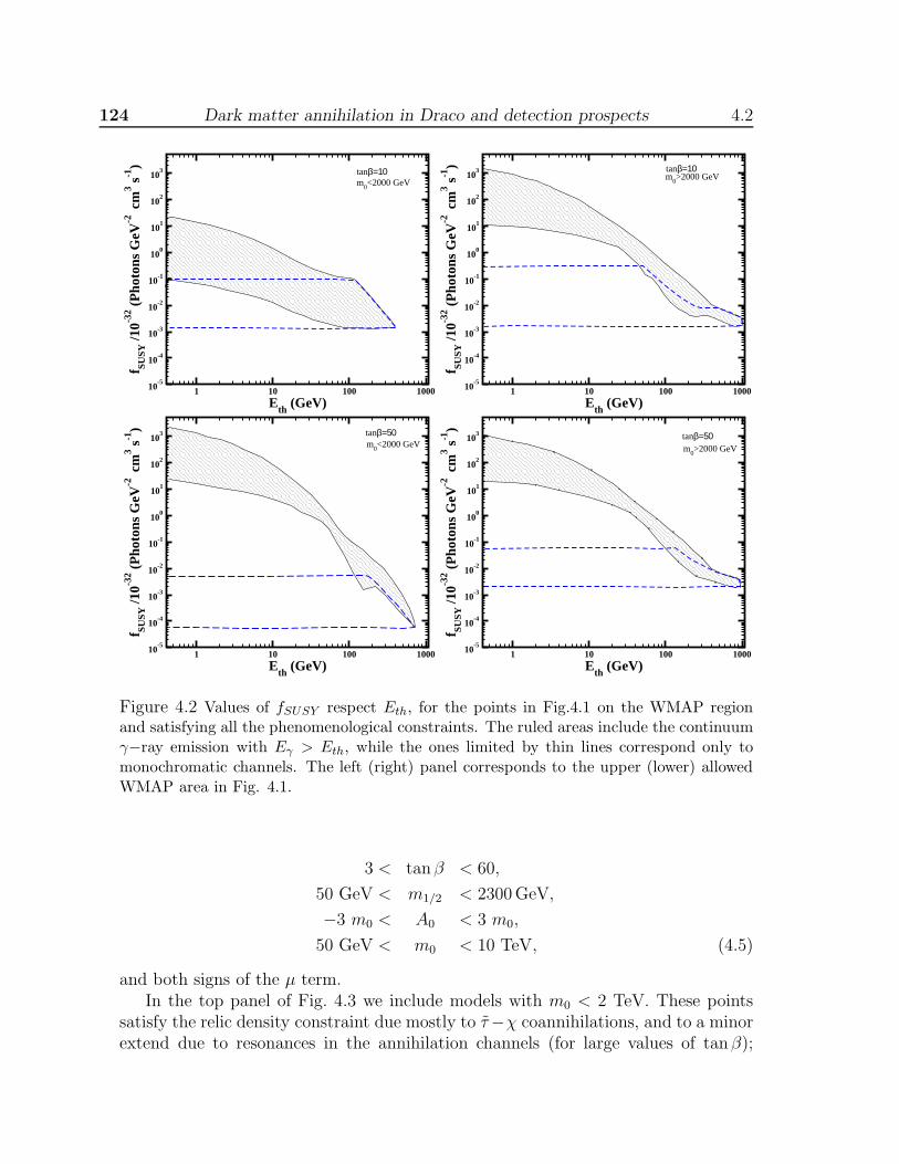
124 Dark matter annihilation in Draco and detection prospects 4.2
1 10 100 1000Eth (GeV)
10-5
10-4
10-3
10-2
10-1
100
101
102
103
f SUSY
/10-3
2 (P
hoto
ns G
eV-2
cm
3 s-1
)
tanβ=10m
0<2000 GeV
1 10 100 1000Eth (GeV)
10-5
10-4
10-3
10-2
10-1
100
101
102
103
f SUSY
/10-3
2 (P
hoto
ns G
eV-2
cm
3 s-1
) tanβ=10m
0>2000 GeV
1 10 100 1000Eth (GeV)
10-5
10-4
10-3
10-2
10-1
100
101
102
103
f SUSY
/10-3
2 (P
hoto
ns G
eV-2
cm
3 s-1
) tanβ=50m
0<2000 GeV
1 10 100 1000Eth (GeV)
10-5
10-4
10-3
10-2
10-1
100
101
102
103
f SUSY
/10-3
2 (P
hoto
ns G
eV-2
cm
3 s-1
)tanβ=50m
0>2000 GeV
Figure 4.2 Values of fSUSY respect Eth, for the points in Fig.4.1 on the WMAP regionand satisfying all the phenomenological constraints. The ruled areas include the continuumγ−ray emission with Eγ > Eth, while the ones limited by thin lines correspond only tomonochromatic channels. The left (right) panel corresponds to the upper (lower) allowedWMAP area in Fig. 4.1.
3 < tanβ < 60,
50 GeV < m1/2 < 2300 GeV,
−3 m0 < A0 < 3 m0,
50 GeV < m0 < 10 TeV, (4.5)
and both signs of the µ term.In the top panel of Fig. 4.3 we include models with m0 < 2 TeV. These points
satisfy the relic density constraint due mostly to τ−χ coannihilations, and to a minorextend due to resonances in the annihilation channels (for large values of tanβ);
4.2 The γ-ray flux in IACTs 125
Figure 4.3 Values of nγ < σχχv > in cm3/s including continuum emission for Eγ > 1 GeV(circles), Eγ > 100 GeV (stars), and considering only the two monochromatic channels(plus).
mχ remain below 700 GeV in this panel. The continuum emission dominates forEγ > 1 GeV, while for Eγ > 100 GeV we find points where the continuum productionis of the same order as the monochromatic γ’s. The bottom panel of Fig. 4.3 containsmodels m0 > 2 TeV. These correspond mostly to the hyperbolic branch region; alsowe can appreciate that larger values for mχ are allowed in this area than in thetop panel. The points with larger cross sections in both panels corresponds to the
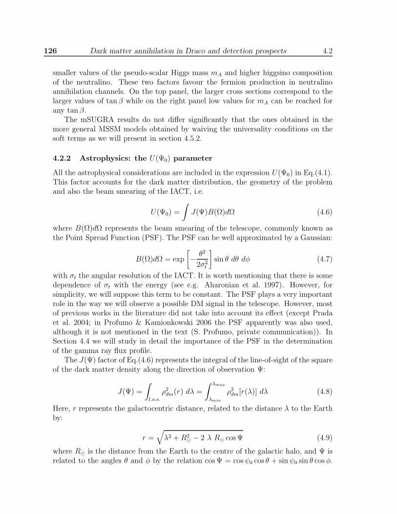
126 Dark matter annihilation in Draco and detection prospects 4.2
smaller values of the pseudo-scalar Higgs mass mA and higher higgsino compositionof the neutralino. These two factors favour the fermion production in neutralinoannihilation channels. On the top panel, the larger cross sections correspond to thelarger values of tanβ while on the right panel low values for mA can be reached forany tanβ.
The mSUGRA results do not differ significantly that the ones obtained in themore general MSSM models obtained by waiving the universality conditions on thesoft terms as we will present in section 4.5.2.
4.2.2 Astrophysics: the U(Ψ0) parameter
All the astrophysical considerations are included in the expression U(Ψ0) in Eq.(4.1).This factor accounts for the dark matter distribution, the geometry of the problemand also the beam smearing of the IACT, i.e.
U(Ψ0) =
∫
J(Ψ)B(Ω)dΩ (4.6)
where B(Ω)dΩ represents the beam smearing of the telescope, commonly known asthe Point Spread Function (PSF). The PSF can be well approximated by a Gaussian:
B(Ω)dΩ = exp
[
− θ2
2σ2t
]
sin θ dθ dφ (4.7)
with σt the angular resolution of the IACT. It is worth mentioning that there is somedependence of σt with the energy (see e.g. Aharonian et al. 1997). However, forsimplicity, we will suppose this term to be constant. The PSF plays a very importantrole in the way we will observe a possible DM signal in the telescope. However, mostof previous works in the literature did not take into account its effect (except Pradaet al. 2004; in Profumo & Kamionkowski 2006 the PSF apparently was also used,although it is not mentioned in the text (S. Profumo, private communication)). InSection 4.4 we will study in detail the importance of the PSF in the determinationof the gamma ray flux profile.
The J(Ψ) factor of Eq.(4.6) represents the integral of the line-of-sight of the squareof the dark matter density along the direction of observation Ψ:
J(Ψ) =
∫
l.o.s.
ρ2dm(r) dλ =
∫ λmax
λmin
ρ2dm[r(λ)] dλ (4.8)
Here, r represents the galactocentric distance, related to the distance λ to the Earthby:
r =√
λ2 +R2⊙ − 2 λ R⊙ cos Ψ (4.9)
where R⊙ is the distance from the Earth to the centre of the galactic halo, and Ψ isrelated to the angles θ and φ by the relation cos Ψ = cosψ0 cos θ + sinψ0 sin θ cosφ.
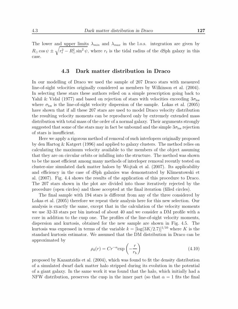
4.3 Dark matter distribution in Draco 127
The lower and upper limits λmin and λmax in the l.o.s. integration are given by
R⊙ cosψ ±√
r2t − R2
⊙ sin2 ψ, where rt is the tidal radius of the dSph galaxy in thiscase.
4.3 Dark matter distribution in Draco
In our modelling of Draco we used the sample of 207 Draco stars with measuredline-of-sight velocities originally considered as members by Wilkinson et al. (2004).In selecting these stars these authors relied on a simple prescription going back toYahil & Vidal (1977) and based on rejection of stars with velocities exceeding 3σlos
where σlos is the line-of-sight velocity dispersion of the sample. Lokas et al. (2005)have shown that if all these 207 stars are used to model Draco velocity distributionthe resulting velocity moments can be reproduced only by extremely extended massdistribution with total mass of the order of a normal galaxy. Their arguments stronglysuggested that some of the stars may in fact be unbound and the simple 3σlos rejectionof stars is insufficient.
Here we apply a rigorous method of removal of such interlopers originally proposedby den Hartog & Katgert (1996) and applied to galaxy clusters. The method relies oncalculating the maximum velocity available to the members of the object assumingthat they are on circular orbits or infalling into the structure. The method was shownto be the most efficient among many methods of interloper removal recently tested oncluster-size simulated dark matter haloes by Wojtak et al. (2007). Its applicabilityand efficiency in the case of dSph galaxies was demonstrated by Klimentowski etal. (2007). Fig. 4.4 shows the results of the application of this procedure to Draco.The 207 stars shown in the plot are divided into those iteratively rejected by theprocedure (open circles) and those accepted at the final iteration (filled circles).
The final sample with 194 stars is different from any of the three considered byLokas et al. (2005) therefore we repeat their analysis here for this new selection. Ouranalysis is exactly the same, except that in the calculation of the velocity momentswe use 32-33 stars per bin instead of about 40 and we consider a DM profile with acore in addition to the cusp one. The profiles of the line-of-sight velocity moments,dispersion and kurtosis, obtained for the new sample are shown in Fig. 4.5. Thekurtosis was expressed in terms of the variable k = [log(3K/2.7)]1/10 where K is thestandard kurtosis estimator. We assumed that the DM distribution in Draco can beapproximated by
ρd(r) = Cr−αexp
(
− r
rb
)
(4.10)
proposed by Kazantzidis et al. (2004), which was found to fit the density distributionof a simulated dwarf dark matter halo stripped during its evolution in the potentialof a giant galaxy. In the same work it was found that the halo, which initially had aNFW distribution, preserves the cusp in the inner part (so that α = 1 fits the final
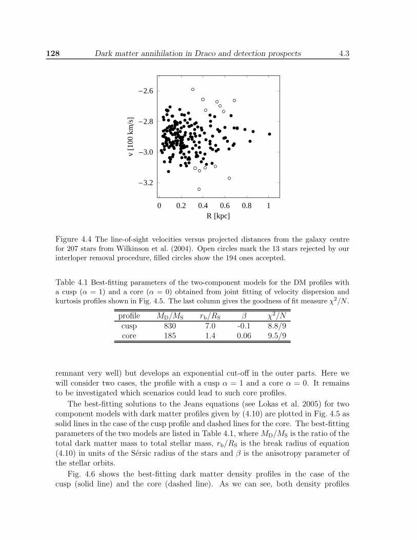
128 Dark matter annihilation in Draco and detection prospects 4.3
0 0.2 0.4 0.6 0.8 1R @kpcD
-3.2
-3.0
-2.8
-2.6
v@1
00kmsD
Figure 4.4 The line-of-sight velocities versus projected distances from the galaxy centrefor 207 stars from Wilkinson et al. (2004). Open circles mark the 13 stars rejected by ourinterloper removal procedure, filled circles show the 194 ones accepted.
Table 4.1 Best-fitting parameters of the two-component models for the DM profiles witha cusp (α = 1) and a core (α = 0) obtained from joint fitting of velocity dispersion andkurtosis profiles shown in Fig. 4.5. The last column gives the goodness of fit measure χ2/N .
profile MD/MS rb/RS β χ2/Ncusp 830 7.0 -0.1 8.8/9core 185 1.4 0.06 9.5/9
remnant very well) but develops an exponential cut-off in the outer parts. Here wewill consider two cases, the profile with a cusp α = 1 and a core α = 0. It remainsto be investigated which scenarios could lead to such core profiles.
The best-fitting solutions to the Jeans equations (see Lokas et al. 2005) for twocomponent models with dark matter profiles given by (4.10) are plotted in Fig. 4.5 assolid lines in the case of the cusp profile and dashed lines for the core. The best-fittingparameters of the two models are listed in Table 4.1, where MD/MS is the ratio of thetotal dark matter mass to total stellar mass, rb/RS is the break radius of equation(4.10) in units of the Sersic radius of the stars and β is the anisotropy parameter ofthe stellar orbits.
Fig. 4.6 shows the best-fitting dark matter density profiles in the case of thecusp (solid line) and the core (dashed line). As we can see, both density profiles
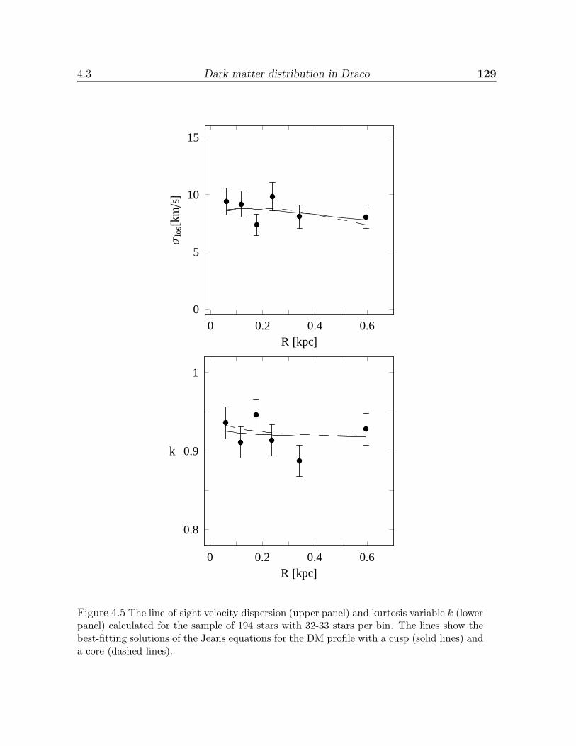
4.3 Dark matter distribution in Draco 129
0 0.2 0.4 0.6R @kpcD
0.8
0.9
1
k
0 0.2 0.4 0.6R @kpcD
0
5
10
15
Σlo
s@kmsD
Figure 4.5 The line-of-sight velocity dispersion (upper panel) and kurtosis variable k (lowerpanel) calculated for the sample of 194 stars with 32-33 stars per bin. The lines show thebest-fitting solutions of the Jeans equations for the DM profile with a cusp (solid lines) anda core (dashed lines).
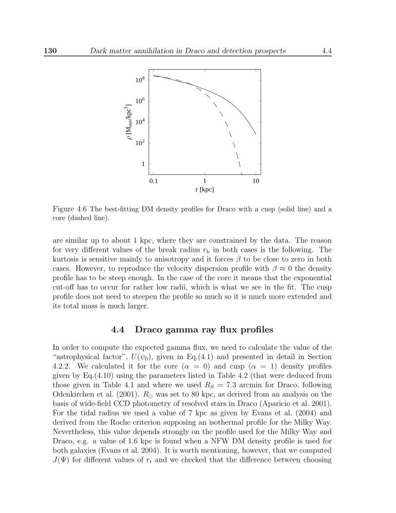
130 Dark matter annihilation in Draco and detection prospects 4.4
0.1 1 10r @kpcD
1
102
104
106
108
Ρ@M
sun
kpc3 D
Figure 4.6 The best-fitting DM density profiles for Draco with a cusp (solid line) and acore (dashed line).
are similar up to about 1 kpc, where they are constrained by the data. The reasonfor very different values of the break radius rb in both cases is the following. Thekurtosis is sensitive mainly to anisotropy and it forces β to be close to zero in bothcases. However, to reproduce the velocity dispersion profile with β ≈ 0 the densityprofile has to be steep enough. In the case of the core it means that the exponentialcut-off has to occur for rather low radii, which is what we see in the fit. The cuspprofile does not need to steepen the profile so much so it is much more extended andits total mass is much larger.
4.4 Draco gamma ray flux profiles
In order to compute the expected gamma flux, we need to calculate the value of the“astrophysical factor”, U(ψ0), given in Eq.(4.1) and presented in detail in Section4.2.2. We calculated it for the core (α = 0) and cusp (α = 1) density profilesgiven by Eq.(4.10) using the parameters listed in Table 4.2 (that were deduced fromthose given in Table 4.1 and where we used RS = 7.3 arcmin for Draco, followingOdenkirchen et al. (2001). R⊙ was set to 80 kpc, as derived from an analysis on thebasis of wide-field CCD photometry of resolved stars in Draco (Aparicio et al. 2001).For the tidal radius we used a value of 7 kpc as given by Evans et al. (2004) andderived from the Roche criterion supposing an isothermal profile for the Milky Way.Nevertheless, this value depends strongly on the profile used for the Milky Way andDraco, e.g. a value of 1.6 kpc is found when a NFW DM density profile is used forboth galaxies (Evans et al. 2004). It is worth mentioning, however, that we computedJ(Ψ) for different values of rt and we checked that the difference between choosing
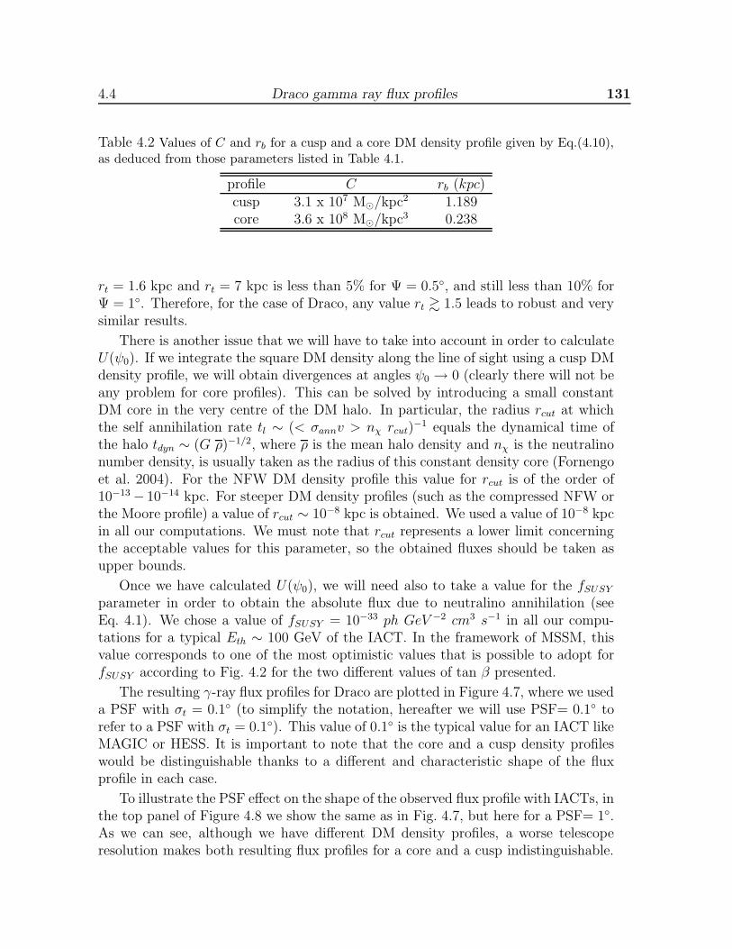
4.4 Draco gamma ray flux profiles 131
Table 4.2 Values of C and rb for a cusp and a core DM density profile given by Eq.(4.10),as deduced from those parameters listed in Table 4.1.
profile C rb (kpc)cusp 3.1 x 10⁷ M⊙/kpc2 1.189core 3.6 x 10⁸ M⊙/kpc3 0.238
rt = 1.6 kpc and rt = 7 kpc is less than 5% for Ψ = 0.5, and still less than 10% forΨ = 1. Therefore, for the case of Draco, any value rt & 1.5 leads to robust and verysimilar results.
There is another issue that we will have to take into account in order to calculateU(ψ0). If we integrate the square DM density along the line of sight using a cusp DMdensity profile, we will obtain divergences at angles ψ0 → 0 (clearly there will not beany problem for core profiles). This can be solved by introducing a small constantDM core in the very centre of the DM halo. In particular, the radius rcut at whichthe self annihilation rate tl ∼ (< σannv > nχ rcut)
−1 equals the dynamical time ofthe halo tdyn ∼ (G ρ)−1/2, where ρ is the mean halo density and nχ is the neutralinonumber density, is usually taken as the radius of this constant density core (Fornengoet al. 2004). For the NFW DM density profile this value for rcut is of the order of10−13 − 10−14 kpc. For steeper DM density profiles (such as the compressed NFW orthe Moore profile) a value of rcut ∼ 10−8 kpc is obtained. We used a value of 10−8 kpcin all our computations. We must note that rcut represents a lower limit concerningthe acceptable values for this parameter, so the obtained fluxes should be taken asupper bounds.
Once we have calculated U(ψ0), we will need also to take a value for the fSUSY
parameter in order to obtain the absolute flux due to neutralino annihilation (seeEq. 4.1). We chose a value of fSUSY = 10−33 ph GeV −2 cm3 s−1 in all our compu-tations for a typical Eth ∼ 100 GeV of the IACT. In the framework of MSSM, thisvalue corresponds to one of the most optimistic values that is possible to adopt forfSUSY according to Fig. 4.2 for the two different values of tan β presented.
The resulting γ-ray flux profiles for Draco are plotted in Figure 4.7, where we useda PSF with σt = 0.1 (to simplify the notation, hereafter we will use PSF= 0.1 torefer to a PSF with σt = 0.1). This value of 0.1 is the typical value for an IACT likeMAGIC or HESS. It is important to note that the core and a cusp density profileswould be distinguishable thanks to a different and characteristic shape of the fluxprofile in each case.
To illustrate the PSF effect on the shape of the observed flux profile with IACTs, inthe top panel of Figure 4.8 we show the same as in Fig. 4.7, but here for a PSF= 1.As we can see, although we have different DM density profiles, a worse telescoperesolution makes both resulting flux profiles for a core and a cusp indistinguishable.

132 Dark matter annihilation in Draco and detection prospects 4.4
Figure 4.7 Draco flux predictions for the core (dashed line) and cusp (solid line) densityprofiles, computed for a typical IACT with Eth = 100 GeV and a PSF= 0.1. We usedfSUSY = 10−33 ph GeV −2 cm3 s−1 (see text for details).
We may think that we could distinguish them from the value of the absolute flux.However, the difference in the absolute flux between both DM density profiles isvery small and in practice the distinction would be impossible. There are manyuncertainties in this absolute flux coming from the particle physics. fSUSY may bevery different from the most optimistic case assumed here, since it could vary morethan three orders of magnitude for this SUSY model (see Fig. 4.2). On the otherhand, the uncertainty in flux due to the DM density profile to be core or cusp isnegligible at least in the inner 0.5 degrees.
Concerning the effect of the PSF given the same DM density profile, a worsetelescope resolution flattens the flux profile as expected. It can be clearly seen in thebottom panel of Figure 4.8, where we plot the Draco γ-ray flux predictions only forthe cusp density profile but using two different values of the PSF (0.1 and 1), andwhere we plot also the same flux profile computed without PSF for comparison.
A good example to show the real importance of the telescope resolution can befound around the controversy generated in the wake of the Draco γ-ray excess reportedby the CACTUS collaboration in 2005 (Marleau 2005). At this moment, it seemsclear that this excess was not real and was probably due to instrumental and trigger-related issues. However, concerning our line of work and always just with the intentionof clarifying the role of the PSF, we must mention the results shown in Profumo &Kamionkowski (2006). There, the CACTUS data were superimposed on different fluxprofiles (each of them related to possible models of DM density profiles for Draco)in Figure 2. These flux profiles were computed using an angular resolution of 0.1,whereas the CACTUS PSF is quite worse than that (around 0.3 for the Crab and

4.4 Draco gamma ray flux profiles 133
Figure 4.8 Top panel: Draco flux predictions for the core (dashed line) and cusp (solidline) density profiles, computed using a PSF= 1. Bottom panel: Draco flux predictionsfor the cusp density profile using two different PSFs. Solid line corresponds to PSF=0.1
and dashed line to PSF=1. The flux profile computing without PSF is also shown forcomparison (dot-dashed line).
probably worse for Draco (Profumo & Kamionkowski 2006; Cactus Collaborationwebpage2). Looking at that figure (despite the authors’ indication to take it with care)one may come to the conclusion that a core profile seems to be the most adequateDM density profile for Draco, as opposed to the cusp profile. However, it would bemore appropriate to make this comparison between the CACTUS data and the fluxprofiles using in both cases the same PSF of the experiment. Doing so and taking
2http://ucdcms.ucdavis.edu/solar2/index.php
134 Dark matter annihilation in Draco and detection prospects 4.5
into account the PSF effect properly, it would be difficult to use the CACTUS datato discriminate between different models for the DM density profile as described in(Profumo & Kamionkowski 2006), since all of the resultant flux profiles would haveessentially the same shape. Only the absolute flux could give us a clue to makethis distinction possible, but as already mentioned there are too many uncertaintiesrelated to an absolute value to be able to extract solid conclusions.
4.5 Detection prospects for some current or plannedexperiments
4.5.1 Flux profile detection
Would it be possible to detect a signal due to neutralino annihilation in Draco usingpresent or planned IACTs and satellite-based gamma ray experiments? Althoughthere are many uncertainties concerning both particle physics and astrophysical is-sues, as already pointed out, it is possible (and necessary) to make some calculations.These calculations will allow us to estimate at least the order of magnitude of theflux that we could expect in our telescopes, and will help us learn which instrumentis, in principle, the best positioned and optimised to detect a possible signal fromDraco.
Draco is located in the northern hemisphere, more precisely at declination 58. Be-cause of that, and regarding currently operating IACTs, MAGIC (Lorentz et al. 2004)and VERITAS (Weekes et al. 2002) are the best options thanks to their geographicalposition. Since both experiments have comparable sensitivity and PSF, we will focusonly on MAGIC. For this IACT, with an energy threshold around 50 GeV for zenithobservations, Draco could be observed 61 above the horizon, so an energy threshold∼ 100 GeV seems to be still possible at that altitude.
Concerning Fermi (Gehrels & Michelson 1999), this satellite-based experimentis designed for making observations of celestial gamma-ray sources in the energyband extending from ∼ 10 MeV to 300 GeV, which is complementary to the one forMAGIC. Moreover, it has a PSF ∼ 0.1 at 10 GeV, which makes this instrument verycompetitive also in DM searches. Fermi was successfully launched in June, 2008.
The flux profiles detection prospects for both gamma-ray experiments can be seenin Figure 4.9, where the lines of sensitivity for MAGIC and Fermi are superimposedon the flux profile computed using the cusp DM density profile for Draco as given byEq.(4.10) together with the parameters listed in Table 4.2. For the case of MAGIC,the sensitivity line represents 250 hours of observation time and a 5σ detection level.As pointed out before, this curve should be comparable and valid for VERITASexperiment as well. Concerning the predicted sensitivity for Fermi, it was calculatedby the Fermi team (see the Fermi webpage3) for 1 year of observation and a 5σ
3http://www-glast.stanford.edu/
4.5 Detection prospects for some current or planned experiments 135
detection level. Values of fSUSY = 10−33 ph GeV−2 cm3 s−1 at 100 GeV (MAGIC)and fSUSY = 1 ·10−29 ph GeV−2 cm3 s−1 at 1 GeV (Fermi) were chosen to convert thevalues calculated from the astrophysical factor U(Ψ0) to flux. These values of fSUSY
correspond to the most optimistic values compatible with that shown in Fig. 4.2. Wechose Eth = 1 GeV for Fermi to be sure that we will have a good angular resolutionfor the arriving photons and also to avoid some uncertainties at low energies in theresponse of the Fermi LAT detector as pointed out in Bertone et al. (2006).
From Figure 4.9 we can see that the detection of the gamma ray flux profile due toneutralino annihilation in Draco with the MAGIC telescope seems to be impossible(at least for the DM density profiles and the particle physics model used here), sincewe would need roughly five orders of magnitude more sensitivity than that reachedby this instrument in a reasonable time to have at least one opportunity to detect apossible signal coming from DM annihilation. For the case of Fermi we obtain moreor less the same, although in this case the expectations are substantially better andwe would need three orders of magnitude more sensitivity. We must note that thisis the most optimistic scenario, so even leaving space to take into account the largeuncertainties coming from the particle physics it seems very hard to have any chanceof detection. In fact, in case of adopting a pessimistic value for fSUSY , the γ-rayflux profile shown in Fig. 4.9 could decrease in more than three orders of magnitudeeasily.
There are some issues concerning a possible detection of DM annihilation not onlyin Draco but also in any other possible target that should be taken into account atthis moment. In the case of a positive detection, this signal would be diffuse (i.e.no point-like source) for an instrument with a PSF good enough. This fact and thecharacteristic spectrum of the source represent the best clues to distinguish betweena γ-ray signal due to neutralino annihilation from other astrophysical sources. Inthe case of Draco, however, we are very far from obtaining any of these clues, soDraco does not seem a good target for DM searches for current or planned γ-rayexperiments (MAGIC-II, for example, will have a factor of 2 more sensitivity thanthe single MAGIC telescope (Baixeras et al. 2005), still clearly insufficient, and thesame improvement in sensitivity is reached in the case of the Fermi satellite if weobserve 5 years instead of 1).
4.5.2 Excess signal detection
Although it is strongly recommendable to try to detect the gamma ray flux profile dueto neutralino annihilation, we could also search only for a gamma ray excess signalin the direction of Draco with a DM origin. In this case the prospects should besomewhat better, since we are only interested in flux detectability (i.e. no interestedin observing an extended emission or not; no discrimination between different fluxprofiles). Draco is around 2 in the sky (the whole DM halo), and one MAGICpointing is 4x 4, so the whole galaxy is within one of these MAGIC pointings. This

136 Dark matter annihilation in Draco and detection prospects 4.5
Figure 4.9 Draco flux profile detection prospects for MAGIC (top panel) and Fermi (bottompanel). The flux profile (solid line) corresponds to the cusp density profile given in Table 4.2and using a PSF=0.1. The sensitivity lines for both instruments were computed for a 5σdetection level and 250 hours (MAGIC) / 1 year (Fermi) of integration time. These figuresshould be taken as the most optimistic case, since we used the most optimistic scenariofrom particle physics in each case. We adopt Eth = 100 GeV for MAGIC and Eth = 1 GeVfor Fermi. See text for details.
means that, to calculate the prospects of an excess signal detection for MAGIC, wemust sum the gamma ray fluxes coming from all the neutralino annihilations thatoccur in the entire halo of the dSph. The same is valid for the case of Fermi, since oneof the main objectives of this mission will be to survey the whole sky, so Draco as awhole will be observed. Nevertheless, most of the γ-ray flux due to DM annihilationcomes from the inner regions of the dwarf, so it would be better to integrate the
4.5 Detection prospects for some current or planned experiments 137
flux and make all the calculations only for those regions. Otherwise, if we integrateup to very large angles from the center, we would be increasing the noise in a largeamount without practically increasing the γ-ray signal, since the gamma ray fluxprofile decreases very rapidly from the center to the outskirts.
We would like here to take the opportunity to mention GAW (Maccarone etal. 2005), which is a R&D path-finder experiment, still under development, for widefield γ-ray astronomy. GAW will operate above 0.7 TeV and will have a PSF ∼ 0.2.It will consist of three identical telescopes working in stereoscopic mode (80m side).The main goal of GAW is to test the feasibility of a new generation of IACTs, whichjoin high sensitivity with large field of view (24 x 24). GAW is planned to be locatedat Calar Alto Observatory (Spain) and a first part of the array should be completedand start to operate during 2008. It is a collaborative effort of research Institutesin Italy, Portugal, and Spain. We will also present some calculations concerningthe possibility to observe a γ-ray signal in the direction of Draco by GAW, just toillustrate the capabilities of the instrument. Nevertheless, the main advantages ofGAW will point to other directions, e.g. the possibility to survey a large portion ofthe sky in a reasonable time above 0.7 TeV.
In Table 4.3 we show the prospects of an excess signal detection (5σ level) forMAGIC, Fermi and GAW and for the case of the cusp DM density profile. Boththe integrated absolute fluxes for Draco and the values given for the sensitivities (i.e.the minimum detectable flux, Fmin) refer to the inner 0.5 of the galaxy (althoughthe total size of Draco in the sky is ∼ 2), just to improve the signal to noise ratioas explained above. The integrated absolute flux for Draco is not the same for thethree experiments, since the fSUSY parameter depends on the energy threshold ofeach instrument, which is different (we chose 100 GeV for MAGIC, 1 GeV for Fermiand 700 GeV for GAW). We did the calculations for the most optimistic case (i.e. thehighest value of fSUSY that we could adopt in the MSSM scenario following Fig. 4.2,and given the energy threshold of each telescope) and the most pessimistic one (thelowest fSUSY ).
According to Table 4.3, an excess signal detection would be impossible with anyof these three instruments, since even in the most optimistic cases they do not reachthe required sensitivity by far. If we compare these numbers with the maximumfluxes shown in Fig.4.9, we can see that the enhancement, although relevant (roughlya factor of 4 in the best case), is still very insufficient for a successful detection.
Moreover, from the results shown in Table 4.3 it becomes really hard to extractany useful results that would help us understand at least a bit better the problemof the dark matter. Indeed, if we observe Draco with MAGIC or Fermi and we donot detect any excess signal, we will not be able to put any useful constraints onthe particle physics involved. None of the actual allowed values for fSUSY could berejected if we find no detection. This makes Draco even less attractive for thosecurrent gamma ray experiments that try to find DM traces.
This can be clearly seen in Fig. 4.10, where we show the parts of the SUSY
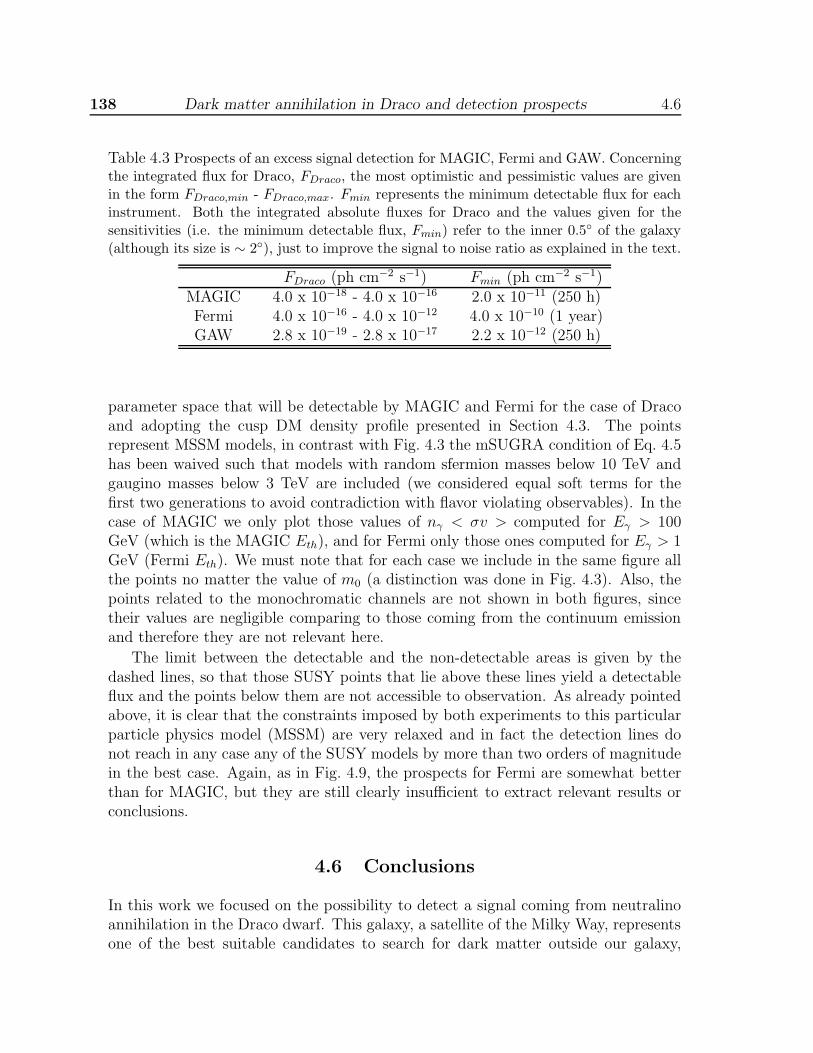
138 Dark matter annihilation in Draco and detection prospects 4.6
Table 4.3 Prospects of an excess signal detection for MAGIC, Fermi and GAW. Concerningthe integrated flux for Draco, FDraco, the most optimistic and pessimistic values are givenin the form FDraco,min - FDraco,max. Fmin represents the minimum detectable flux for eachinstrument. Both the integrated absolute fluxes for Draco and the values given for thesensitivities (i.e. the minimum detectable flux, Fmin) refer to the inner 0.5 of the galaxy(although its size is ∼ 2), just to improve the signal to noise ratio as explained in the text.
FDraco (ph cm−2 s−1) Fmin (ph cm−2 s−1)MAGIC 4.0 x 10⁻¹⁸ - 4.0 x 10⁻¹⁶ 2.0 x 10⁻¹¹ (250 h)Fermi 4.0 x 10⁻¹⁶ - 4.0 x 10⁻¹² 4.0 x 10⁻¹⁰ (1 year)GAW 2.8 x 10⁻¹⁹ - 2.8 x 10⁻¹⁷ 2.2 x 10⁻¹² (250 h)
parameter space that will be detectable by MAGIC and Fermi for the case of Dracoand adopting the cusp DM density profile presented in Section 4.3. The pointsrepresent MSSM models, in contrast with Fig. 4.3 the mSUGRA condition of Eq. 4.5has been waived such that models with random sfermion masses below 10 TeV andgaugino masses below 3 TeV are included (we considered equal soft terms for thefirst two generations to avoid contradiction with flavor violating observables). In thecase of MAGIC we only plot those values of nγ < σv > computed for Eγ > 100GeV (which is the MAGIC Eth), and for Fermi only those ones computed for Eγ > 1GeV (Fermi Eth). We must note that for each case we include in the same figure allthe points no matter the value of m0 (a distinction was done in Fig. 4.3). Also, thepoints related to the monochromatic channels are not shown in both figures, sincetheir values are negligible comparing to those coming from the continuum emissionand therefore they are not relevant here.
The limit between the detectable and the non-detectable areas is given by thedashed lines, so that those SUSY points that lie above these lines yield a detectableflux and the points below them are not accessible to observation. As already pointedabove, it is clear that the constraints imposed by both experiments to this particularparticle physics model (MSSM) are very relaxed and in fact the detection lines donot reach in any case any of the SUSY models by more than two orders of magnitudein the best case. Again, as in Fig. 4.9, the prospects for Fermi are somewhat betterthan for MAGIC, but they are still clearly insufficient to extract relevant results orconclusions.
4.6 Conclusions
In this work we focused on the possibility to detect a signal coming from neutralinoannihilation in the Draco dwarf. This galaxy, a satellite of the Milky Way, representsone of the best suitable candidates to search for dark matter outside our galaxy,

4.6 Conclusions 139
100 200 300 400 500 600 700 800 900 1000mχ (GeV)
10-4
10-3
10-2
10-1
100
101
102
103
104
105
106
107
108
n γ <σ
v>/1
0-29
( cm
3 s-1
)
100 200 300 400 500 600 700 800 900 1000mχ (GeV)
10-4
10-3
10-2
10-1
100
101
102
103
104
105
106
107
108
n γ <σ
v>/1
0-29
( cm
3 s-1
)
Figure 4.10 Exclusion limits for MAGIC (upper panel) and Fermi (bottom panel), forcontinuum γ-ray emission above 100 GeV (MAGIC) and 1 GeV (Fermi). The lines representfor each instrument the minimum detectable nγ < σv > adopting the cusp DM densityprofile given in Table 4.2 for Draco. We used 250 hours (1 year) of integration time forMAGIC (Fermi) and a 5σ detection level. Below the lines, the SUSY models (points) donot yield a flux high enough for a successful detection. According to these plots, neitherMAGIC nor Fermi may put any useful constraints at least to this particular particle physicsmodel.
since it is near and it has probably more observational constraints than any otherknown dark matter dominated system. This fact becomes crucial when we want
140 Dark matter annihilation in Draco and detection prospects 4.6
to make realistic predictions of the expected observed γ-ray flux due to neutralinoannihilation.
Draco is a dwarf galaxy tidally stripped by the Milky Way, so it seems preferableto build a model for the mass distribution that takes into account this importantfact. Using this more appropriate model for Draco, we have obtained the γ-ray fluxprofiles for the case of a cusp and a core DM density profiles (both scenarios areequally valid according to the observations). To do that, we first estimated the best-fitting parameters for each density profile by adjusting the solutions of the Jeansequations to velocity moments obtained for the Draco stellar sample cleaned by arigorous method of interloper removal. Apart from this recommendable and usefulupdate on the best DM model for Draco, one important conclusion can be extractedconcerning the absolute γ-flux: for both cusp and core DM density profiles, the fluxvalues that we obtain are very similar for the inner region of the dwarf, i.e. where wehave the largest flux values and signal detection would be easier.
There is, however, a way to distinguish between a core and a cusp DM densityprofile. The crucial points concerning this issue are the sensitivity and the PSF ofthe telescope. If the telescope resolution is good enough (and we reach the requiredsensitivity) a distinction between both cusp and core models may be possible thanksto the shape of the flux profile in each case. However, if the PSF of the instrumentis poor, its effect could make it impossible to discriminate between different fluxprofiles, i.e. different models of the DM density profile. In any case, to be sure thatthe signal is due to neutralino annihilation, we will need to have a PSF good enoughto be able to resolve the source (i.e. we will need to detect with a good resolutionat least a portion of the flux profile large enough so we can conclude that it belongsto neutralino annihilation). This fact together with a characteristic spectrum are theunequivocal traces of a DM source. Both issues are of course totally valid not onlyfor Draco but also for any other target, and therefore they should be always takeninto account.
We may think that for Draco the effect of the PSF is not especially important,since current experiments do not seem to reach even the required sensitivity to detecta γ-ray signal coming from the center of the dSph. Indeed, the limiting factor hereis the expected flux and not the PSF of the telescope. Nevertheless, we shouldaccount for the PSF of the instrument in any case, since we do not know a priori theexpected gamma flux and we will not have a realistic prediction unless we includeit in our calculations. Only then we will know the exact shape of the flux profile ascould be observed by the telescope and therefore we can evaluate the real chances ofdetection. Furthermore, we must note that the inclusion of the PSF corresponds toa more general analysis not only valid for Draco but also for any target (the case theMilky Way for example where the role of the PSF is critical to understand the originof the gamma emission in its center).
Some estimations concerning flux profile detection prospects for the MAGIC andFermi experiments have been also shown. According to these calculations, even in
4.6 Conclusions 141
the most optimistic scenario (i.e. with the highest values of fSUSY allowed for theMSSM particle physics model adopted here) a γ-ray signal detection from Dracoseems to be really hard at least for the current IACTs and for the Fermi satellite. Inaddition, it would be really difficult to improve our expectations for Draco, since forexample larger integration times will not improve drastically the sensitivity lines ofthese instruments up to the level allowing successful detection (we need around fiveand three orders of magnitude more sensitivity for success with MAGIC and Fermirespectively). The uncertainties coming from astrophysics, as already mentioned, arenegligible compared to those coming from the particle physics, so either by choosinga cusp or a core DM density profile for Draco (or even modifying this for a steeperone) we will not be able to increase the γ-ray flux up to the level where we can expecta signal detection.
We also explored the prospects of an excess signal detection (i.e. we are not in-terested in the shape of the gamma ray flux profile, only in detectability) for MAGICand Fermi, but we reached the same strongly negative conclusions as those obtainedfor the flux profile detection. Both instruments are very far from the required sensi-tivity so it seems that they do not have any chance of successful detection. But evenmore, in the case of an (expected) unsuccessful detection we would not be able to putany useful constraints on the particle physics involved (the uncertainties from differ-ent dark matter density profiles and other astrophysical considerations are negligiblecompared to this). None of the actual allowed values for fSUSY could be rejected ifwe find no detection. This makes Draco even less attractive for those current gammaray experiments that try to find DM traces.
From these negative results it seems that, at least for current experiments, Dracodoes not represent a good target for DM searches (although some important enhance-ments mechanisms in the γ-ray signal coming from neutralino annihilation in Dracohave been proposed in Colafrancesco et al. (2007). If we want to find unequivocaltraces of non-barionic dark matter in the Universe, an effort should be done in orderto find other more promising DM targets. In this context, it is interesting to notethat the number of known dSph galaxies satellites of the Milky Way has increasedconsiderably in the last few years, doing possible that some of them may offer moreoptimistic detection prospects than Draco itself (Strigari et al. 2007). A quantitativestudy should be done in this direction. The search of DM subhalos in the solar neigh-borhood (see e.g. Diemand et al. 2007) or exploring the IMBHs scenario (Bertone etal. 2005b) may represent also other challenging possibilities, although these one morespeculative for the moment.
Finally, it is worth mentioning that IACTs that join a large field of view with ahigh sensitivity will represent the future in this field and will provide a next step inDM searches. In this context, the Cherenkov Telescope Array (CTA) project4 willbe specially important, with a threshold energy well below 100 GeV, a wide spectral
4http://www.mpi-hd.mpg.de/hfm/CTA/CTA home.html/

142 Dark matter annihilation in Draco and detection prospects 4.6
coverage up to 100 TeV and a factor of 5-10 more sensitivity than present experimentsin the mentioned range. Also GAW, a R&D experiment under development, with anenergy threshold ∼ 700 GeV and a 24 x 24 field of view, will constitute anothercomplementary attempt in the same direction, although under a different approach.
Bibliography
Aharonian F. A., Hofmann F., Konopelko A. K. and Volk H. J., 1997, Astropart.Phys., 6, 343
Aharonian F. et al. , 2004, A&A, 425, L13
Aharonian F. et al. , 2006, Nature, 439, 695
Aharonian F. et al. , 2006b, Phys. Rev. Letters, 97, 221102
Albert J. et al. , 2006, ApJ, 638, L101
Aparicio A., Carrera R. and Martinez-Delgado D., 2001, AJ, 122, 2524
Baixeras C. et al. , 2005, Proc. of the 29th International Cosmic Ray Conference,ICRC, 5, 227
Belanger G., Boudjema F., Pukhov A. and Semenov A., 2006, Comput. Phys. Com-mun., 174, 577; Comput. Phys. Commun., 2002, 149, 103
Bergstrom L. and Ullio P., 1997, Nucl. Phys. B, 504, 27
Bergstrom L., 2000, Rep. Prog. Phys., 63, 793
Bergstrom L. et al. , 2005, Phys. Rev. Letters, 95, 241301
Bergstrom L. and Hooper D., 2006, Phys. Rev. D, 73, 063510
Bern Z., Gondolo P. and Perelstein M., 1997, Phys. Lett. B, 411, 86
Bertone G., Hooper D. and Silk J., 2005, Physics Reports, 405, 279
Bertone G.. Zentner A. R. and Silk J., 2005b, Phys. Rev. D, 72, 103517
Bertone G., Bringmann T., Rando R., Busetto G. and Morselli A., 2006, preprint,astro-ph/0612387
Cerdeno D. G., Gabrielli E., Gomez M. E.and Munoz C., 2003, JHEP, 0306, 030

144 BIBLIOGRAPHY 4.6
Colafrancesco S., Profumo S. and Ullio P., 2007, Phys. Rev. D, 75, 023513
den Hartog R. and Katgert P., 1996, MNRAS, 279, 349
Diemand J., Kuhlen M. & Madau P., 2007, ApJ, 657, 262
Evans N. W., Ferrer F. and Sarkar S., 2004, Phys. Rev. D, 69, 123501
Fornengo N., Pieri L. and Scopel S., 2004, Phys. Rev. D, 70, 103529
Gehrels N. and Michelson P., 1999, Astropart. Phys., 11, 277
Gomez M. E., Lazarides G. and Pallis C., 2003, Phys. Rev. D, 67, 097701; GomezM. E., Lazarides G. and Pallis C., 2002, Nucl. Phys. B, 638, 165
Gomez M. E., Ibrahim T., Nath P. and Skadhauge S., 2005, Phys. Rev. D, 72,095008
Gomez M. E., Ibrahim T., Nath P. and Skadhauge S., 2006, Phys. Rev. D, 74,015015
Gondolo P., Edsjo J., Ullio P., Bergstrom L., Schelke M. and Baltz E. A., 2004,JCAP, 0407, 008
Hinton J. A., 2004, New Astron. Rev., 48, 331
Kazantzidis S., Mayer L., Mastropietro C., Diemand J., Stadel J. and Moore B.,2004, ApJ, 608, 663
Klimentowski J., Lokas E. L., Kazantzidis S., Prada F., Mayer L. and Mamon G.A., 2007, MNRAS, 378, 353
Kosack K. et al. , 2004, ApJ, 608, L97
Lokas E. L., Mamon G. A. and Prada F., 2005, MNRAS, 363, 918
Lorentz E. et al. , 2004, New Astron. Rev., 48, 339
Maccarone M. C. et al. , 2005, Proc. of the 29th International Cosmic Ray Confer-ence, ICRC, 5, 295
Mambrini Y., Munoz C., Nezri E. and Prada F., 2006, JCAP, 01, 010
Marleau P., TAUP, September 2005, Zaragoza (Spain); Tripathi M., Cosmic Raysto Colliders 2005, Prague (Czech Republic), September 2005; TeV Particle Astro-physics Workshop, Batavia (USA), July 2005; Chertok M., Proc. of Panic 05, SantaFe (USA), October 2005
4.6 BIBLIOGRAPHY 145
Munoz C., 2004, Int. J. Mod. Phys. A, 19, 3093
Odenkirchen M., et al. , 2001, AJ, 122, 2538
Paige F. E, Protopopescu S. D., Baer H. and Tata X., 2003, preprint, hep-ph/0312045.
Prada F., Klypin A., Flix J., Martınez M. and Simonneau E., 2004, Phys. Rev. Lett.,93, 241301
Profumo S., 2006, Phys. Rev. D, 72, 103521
Profumo S. and Kamionkowski M., 2006, JCAP, 3, 3
Spergel D. N. et al. , 2007, ApJS, 170, 377
Stark L. S, Hafliger P., Biland A. and Pauss F., 2005, JHEP, 0508, 059
Strigari, L. E., Koushiappas, S. M., Bullock, J. S., Kaplinghat, M., Simon, J. D.,Geha, M., & Willman, B. 2008, ApJ, 678, 614
Tsuchiya K. et al. , 2004, ApJ, 606, L115
Ullio P. and Bergstrom L., 1998, Phys. Rev. D, 57, 1962
Weekes T. C. et al. , 2002, Astropart. Phys., 17, 221
Wilkinson M. I., Kleyna J. T., Evans N. W, Gilmore G. F., Irwin M. J. and GrebelE. K., 2004, ApJ, 611, L21
Wojtak R., Lokas E. L., Mamon G. A., Gottlober S., Prada F. and Moles M., 2007,A&A, 466, 437
Yahil A. and Vidal N. V., 1977, ApJ, 214, 347

146 BIBLIOGRAPHY 4.6
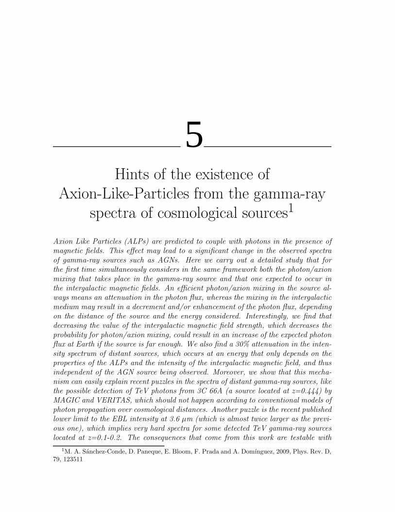
5Hints of the existence of
Axion-Like-Particles from the gamma-ray
spectra of cosmological sources1
Axion Like Particles (ALPs) are predicted to couple with photons in the presence ofmagnetic fields. This effect may lead to a significant change in the observed spectraof gamma-ray sources such as AGNs. Here we carry out a detailed study that forthe first time simultaneously considers in the same framework both the photon/axionmixing that takes place in the gamma-ray source and that one expected to occur inthe intergalactic magnetic fields. An efficient photon/axion mixing in the source al-ways means an attenuation in the photon flux, whereas the mixing in the intergalacticmedium may result in a decrement and/or enhancement of the photon flux, dependingon the distance of the source and the energy considered. Interestingly, we find thatdecreasing the value of the intergalactic magnetic field strength, which decreases theprobability for photon/axion mixing, could result in an increase of the expected photonflux at Earth if the source is far enough. We also find a 30% attenuation in the inten-sity spectrum of distant sources, which occurs at an energy that only depends on theproperties of the ALPs and the intensity of the intergalactic magnetic field, and thusindependent of the AGN source being observed. Moreover, we show that this mecha-nism can easily explain recent puzzles in the spectra of distant gamma-ray sources, likethe possible detection of TeV photons from 3C 66A (a source located at z=0.444) byMAGIC and VERITAS, which should not happen according to conventional models ofphoton propagation over cosmological distances. Another puzzle is the recent publishedlower limit to the EBL intensity at 3.6 µm (which is almost twice larger as the previ-ous one), which implies very hard spectra for some detected TeV gamma-ray sourceslocated at z=0.1-0.2. The consequences that come from this work are testable with
1M. A. Sanchez-Conde, D. Paneque, E. Bloom, F. Prada and A. Domınguez, 2009, Phys. Rev. D,79, 123511

148 Hints of the existence of ALPs from the γ-ray spectra of cosmological sources 5.1
the current generation of gamma-ray instruments, namely Fermi (formerly known asGLAST) and imaging atmospheric Cherenkov telescopes like CANGAROO, HESS,MAGIC and VERITAS.
5.1 Introduction
The existence of axions is predicted by the Peccei-Quinn mechanism, which is cur-rently the most compelling explanation to solve the CP problem in QCD (Peccei &Quinn 1977). Moreover, amongst all the valid candidates proposed to constitute aportion or the totality of the non-barionic cold dark matter content predicted to existin the Universe, hypothetical non-thermal axions, or in a more generic way, Axion-Like Particles (ALPs), where the mass and the coupling constant are not related toeach other, may represent a good option: they might exist in sufficient quantities toaccount for the estimated dark matter density and they might interact very weaklywith the rest of the particles (Raffelt 2005). There is an additional property of ALPsthat makes them even more attractive and that could have important implicationsfor its detectability, i.e. they can oscillate into photons and vice-versa in the presenceof an electric or magnetic field (Dicus et al. 1978, Sikivie et al. 1983). This is analo-gous to that predicted to occur between neutrinos of different flavors, and a similarbehavior is expected in the case of the recently proposed chameleons as well (Bur-rage et al. 2009). This characteristic is the main vehicle used at present to carry outan exhaustive search of ALPs by experiments like CAST (Andriamonje et al. 2007),PVLAS (Zavattini et al. 2006) and ADMX (Duffy et al. 2006).
The oscillation of photons to ALPs (and vice-versa) could have important impli-cations for astronomical observations. This argument was first investigated in theoptical band by Csaki et al. (2002), where authors proposed the existence of axionsto be the cause of the observed supernova Ia dimming. In this context, the observeddimming might be explained as a result of an efficient photon to axion conversioninstead of a cosmic acceleration (albeit this proposal was rejected some time later dueto some chromatic problems, pointed out e.g. by Mirizzi et al. (2008). Photon/axionoscillations were also studied by the same authors in Csaki et al. (2003) as an al-ternative explanation for those photons arriving Earth from very distant sources atenergies above the GZK cutoff.
Recently, it has been proposed that, if ALPs exist, they could distort the spectraof gamma-ray sources, such as Active Galactic Nuclei (AGNs) (Hooper & Serpico2007, De Angelis et al. 2007, Hochmuth & Sigl 2007, Simet et al. 2008) or galacticsources in the TeV range (Mirizzi et al. 2007), and that their effect may be detectedby current gamma-ray experiments. In Burrage et al. (2009b), for example, it isstated that also the scatter in AGN luminosity relations could be used to searchfor ALPs. Other astrophysical environments have been proposed in order to detectALPs, such as the magnetic field of the Sun (Fairbairn et al. 2007), pulsars (Dupayset al. 2005), the galactic halo (Duffy et al. 2006) or GRBs and QSOs by carefully
5.1 Introduction 149
studying their polarized gamma-ray emissions (Rubbia & Sakharov 2008, Hutsemek-ers et al. 2008). In particular, these predictions are very relevant for gamma-rayastronomy, where recent instrumentation developments in the last few years have in-creased the observational capabilities by more than one order of magnitude. On theground, we have the new generation of Imaging Atmospheric Cherenkov Telescopes(IACTs) like MAGIC (Lorentz et al. 2004), HESS (Hinton et al. 2004), VERITAS(Weekes et al. 2002) or CANGAROO-III (Enomoto et al. 2002), covering energies inthe range 0.1-20 TeV. In space we have Fermi (previously called GLAST) (Gehrels &Michelson 1999), in operation since Summer 2008 and covering energies in the range0.02-300 GeV2.
In this work we revisit the photon/axion mixing, for the first time handling underthe same consistent framework the mixing that takes place inside or near the gamma-ray sources together with that one expected to occur in intergalactic magnetic field(IGMF). In the literature, both effects have been considered separately. Depending onthe source dimension, magnetic field, ALP mass and coupling constant, both effectsmight produce significant spectral distortions, or one effect could be more importantthan the other. In any case, we believe that both effects could be relevant and henceneed to be considered simultaneously. We neglect, however, the mixing that mayhappen inside the Milky Way due to galactic magnetic fields. At present, a concisemodeling of this effect is still very dependent on the largely unknown morphologyof the magnetic field in the galaxy. Furthermore, in the most idealistic/optimisticcase, this effect would produce an enhancement of the photon flux arriving at Earthof about 3% of the initial photon flux emitted by the source (Simet et al. 2008).This is in contrast with what we found for the IGMFs: although there is also littleinformation on the strength and morphology of the IGMFs, the derived photon/axionmixing in this case we show to be crucial for a correct interpretation of the observedflux. It is worth mentioning that we will come to this conclusion using a conservativevalue of B=0.1 nG for the IGMF strength, well below the current upper limits of ∼1nG. We also carry out a detailed analysis of the mixing when varying IGMF strengthand source distance. We find results that differ from previously published ones, andwe make predictions of effects that have not been noted in the literature so far.
At energies larger than 10 GeV, and especially above 100 GeV, it will be necessaryto properly account for the Extragalactic Background Light (EBL) in our IGMFmixing calculations. The EBL introduces an attenuation in the photon flux dueto e−e+ pair production that comes from the interaction of the gamma-ray sourcephotons with infrared and optical-UV background photons (Hauser & Dwek 2001).Amongst all the EBL models that exist in the literature, in this work we will make useof the Primack (Primack 2005) and Kneiske best-fit Kneiske et al. 2004) EBL models.They represent respectively one of the most transparent and one of the most opaquemodels for gamma-rays, but still within the limits imposed by the observations. The
2In the space we also have a new gamma-ray instrument called AGILE (Tavani et al. 2008), yetthe sensitivity is actually similar to that of EGRET
150 Hints of the existence of ALPs from the γ-ray spectra of cosmological sources 5.2
EBL model will play a crucial role in our formalism and results: as we will see,the more attenuating the EBL model considered, the more relevant the effect ofphoton/axion oscillations in the IGMF.
We also explore in this work the detection prospects for current gamma-ray in-struments (Fermi and IACTs). We will show that the signatures of photon/axion os-cillations may be observationally detectable provided light ALPs with masses smallerthan a given value for typical values of the IGMF. In order to study the detectionprospects, we will propose an observational strategy. We can anticipate here thatthe main challenge for our proposed formalism to be testable comes from the lack ofknowledge of the intrinsic source spectrum and EBL density. However, we note thatthere is the possibility that we could be already detecting the first hints of axions withcurrent experiments. In this context, the potential detection of TeV photons fromvery distant (z ∼ 0.4) sources (Acciari 2009, Albert et al. 2008, Nesphor et al. 1998,Stepanyan et al. 2002), or some works claiming energy spectral indices harder than1.5 for relatively distant (z=0.1-0.2) AGNs (Krennrich et al. 2008), already put in atight spot the conventional interpretation of the observed gamma-ray data. As wewill show, both effects could be explained by oscillations of photon into light ALPsusing realistic values for the involved parameters.
The work is organized as follows. In Section 5.2 we describe in detail the pho-ton/axion mixing in both the surroundings of gamma-ray sources and in the inter-galactic medium (IGM). Section 5.3 is devoted to present the results obtained whenincluding both mixings under the same framework and after considering realistic pa-rameters for well-known AGNs. In Section 5.4 we present an observational strategyto search for ALPs using the most sensitive gamma-ray instruments, namely Fermiand IACTs like MAGIC or HESS. Finally, we give our conclusions in Section 5.5.
5.2 The formalism
At present, the Peccei-Quinn mechanism remains as the most convincing solution tosolve the CP violation of QCD. As early as in 1978, Weinberg (Weinberg 1978) andWilczek (Wilczek 1978) realized independently that a consequence of this mechanismis the existence of a pseudo-scalar boson, the axion. One generic property of axionsis a two-photon interaction of the form:
Laγ = − 1
4 MFµνF
µνa =
1
ME · B a (5.1)
where a is the axion field, M is the inverse of the photon/axion coupling strength,F is the electromagnetic field-strength tensor, F its dual, E the electric field, andB the magnetic field. The axion has the important feature that its mass ma andcoupling constant are inversely related to each other. There are, however, otherpredicted states where this relation does not hold; such states are known as AxionLike Particles (ALPs). An important and intriguing consequence of Eq. (5.1) is that
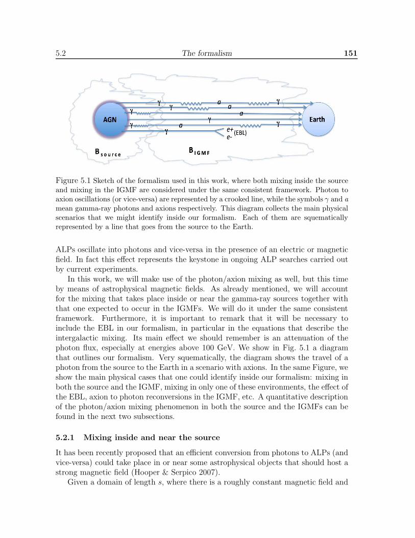
5.2 The formalism 151
Figure 5.1 Sketch of the formalism used in this work, where both mixing inside the sourceand mixing in the IGMF are considered under the same consistent framework. Photon toaxion oscillations (or vice-versa) are represented by a crooked line, while the symbols γ and a
mean gamma-ray photons and axions respectively. This diagram collects the main physicalscenarios that we might identify inside our formalism. Each of them are squematicallyrepresented by a line that goes from the source to the Earth.
ALPs oscillate into photons and vice-versa in the presence of an electric or magneticfield. In fact this effect represents the keystone in ongoing ALP searches carried outby current experiments.
In this work, we will make use of the photon/axion mixing as well, but this timeby means of astrophysical magnetic fields. As already mentioned, we will accountfor the mixing that takes place inside or near the gamma-ray sources together withthat one expected to occur in the IGMFs. We will do it under the same consistentframework. Furthermore, it is important to remark that it will be necessary toinclude the EBL in our formalism, in particular in the equations that describe theintergalactic mixing. Its main effect we should remember is an attenuation of thephoton flux, especially at energies above 100 GeV. We show in Fig. 5.1 a diagramthat outlines our formalism. Very squematically, the diagram shows the travel of aphoton from the source to the Earth in a scenario with axions. In the same Figure, weshow the main physical cases that one could identify inside our formalism: mixing inboth the source and the IGMF, mixing in only one of these environments, the effect ofthe EBL, axion to photon reconversions in the IGMF, etc. A quantitative descriptionof the photon/axion mixing phenomenon in both the source and the IGMFs can befound in the next two subsections.
5.2.1 Mixing inside and near the source
It has been recently proposed that an efficient conversion from photons to ALPs (andvice-versa) could take place in or near some astrophysical objects that should host astrong magnetic field (Hooper & Serpico 2007).
Given a domain of length s, where there is a roughly constant magnetic field and
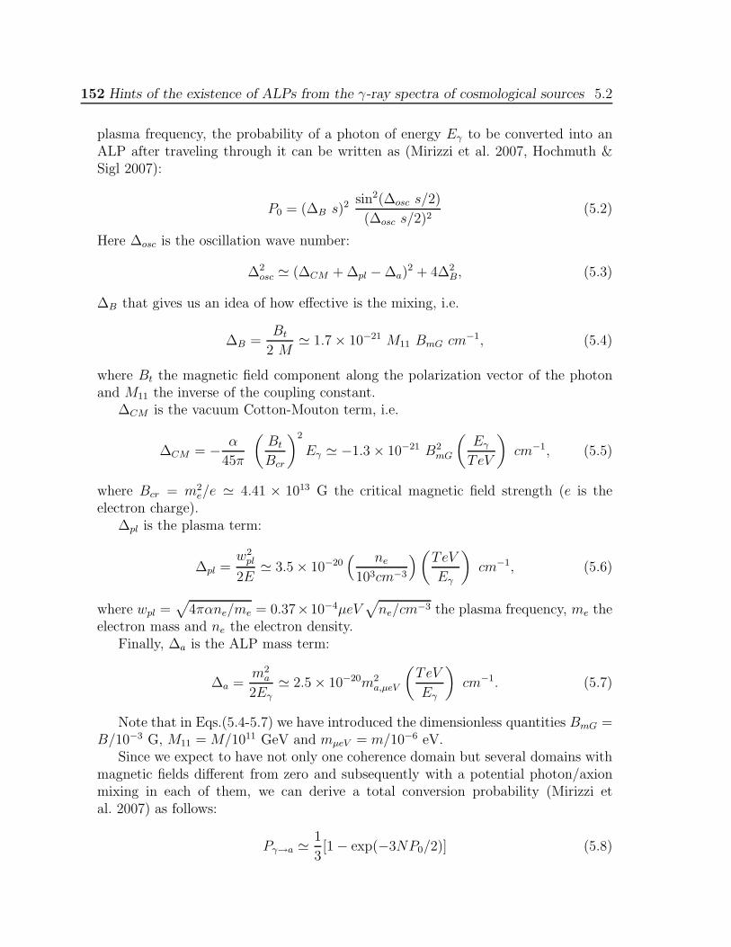
152 Hints of the existence of ALPs from the γ-ray spectra of cosmological sources 5.2
plasma frequency, the probability of a photon of energy Eγ to be converted into anALP after traveling through it can be written as (Mirizzi et al. 2007, Hochmuth &Sigl 2007):
P0 = (∆B s)2 sin2(∆osc s/2)
(∆osc s/2)2(5.2)
Here ∆osc is the oscillation wave number:
∆2osc ≃ (∆CM + ∆pl − ∆a)2 + 4∆2
B, (5.3)
∆B that gives us an idea of how effective is the mixing, i.e.
∆B =Bt
2 M≃ 1.7 × 10⁻²¹ M11 BmG cm−1, (5.4)
where Bt the magnetic field component along the polarization vector of the photonand M11 the inverse of the coupling constant.
∆CM is the vacuum Cotton-Mouton term, i.e.
∆CM = − α
45π
(
Bt
Bcr
)2
Eγ ≃ −1.3 × 10⁻²¹ B2mG
(
Eγ
TeV
)
cm−1, (5.5)
where Bcr = m2e/e ≃ 4.41 × 10¹³ G the critical magnetic field strength (e is the
electron charge).∆pl is the plasma term:
∆pl =w2
pl
2E≃ 3.5 × 10⁻²⁰
( ne
103cm−3
)
(
TeV
Eγ
)
cm−1, (5.6)
where wpl =√
4παne/me = 0.37×10⁻⁴µeV√
ne/cm−3 the plasma frequency, me theelectron mass and ne the electron density.
Finally, ∆a is the ALP mass term:
∆a =m2
a
2Eγ
≃ 2.5 × 10⁻²⁰m2a,µeV
(
TeV
Eγ
)
cm−1. (5.7)
Note that in Eqs.(5.4-5.7) we have introduced the dimensionless quantities BmG =B/10−3 G, M11 = M/1011 GeV and mµeV = m/10−6 eV.
Since we expect to have not only one coherence domain but several domains withmagnetic fields different from zero and subsequently with a potential photon/axionmixing in each of them, we can derive a total conversion probability (Mirizzi etal. 2007) as follows:
Pγ→a ≃ 1
3[1 − exp(−3NP0/2)] (5.8)

5.2 The formalism 153
where P0 is given by Eq.(5.2) and N represents the number of domains. Note thatin the limit where N P0 → ∞, the total probability saturates to 1/3, i.e. one thirdof the photons will convert into ALPs.
It is useful here to rewrite Eq. (5.2) following Hooper & Serpico (2007), i.e.
P0 =1
1 + (Ecrit/Eγ)2sin2
B s
2 M
√
1 +
(
Ecrit
Eγ
)2
(5.9)
so that we can define a characteristic energy, Ecrit, given by:
Ecrit ≡m2 M
2 B(5.10)
or in more convenient units:
Ecrit(GeV ) ≡m2
µeV M11
0.4 BG(5.11)
where the subindices refer again to dimensionless quantities: mµeV ≡ m/µeV , M11 ≡M/1011 GeV andBG ≡ B/Gauss; m is the effective ALP massm2 ≡ |m2
a−ω2pl|. Recent
results from the CAST experiment (Andriamonje et al. 2007) give a value of M11 ≥0.114 for axion mass ma ≤ 0.02 eV. Although there are other limits derived withother methods or experiments, the CAST bound is the most general and stringentlimit in the range 10−11 eV ≪ ma ≪ 10−2 eV.
At energies below Ecrit the conversion probability is small, which means that themixing will be small. Therefore we must focus our detection efforts at energies abovethis Ecrit, where the mixing is expected to be large (strong mixing regime). As pointedout in , in the case of using typical parameters for an AGN in Eq. (5.11), Ecrit willlie in the GeV range given an ALP mass of the order of ∼ µeV.
To illustrate how the photon/axion mixing inside the source works, we show inFigure 5.2 an example for an AGN modeled by the parameters listed in Table 5.2 (ourfiducial model, see Section 5.3). The only difference is the use of an ALP mass of 1µeV instead of the value that appear in that Table, so that we obtain a critical energythat lie in the GeV energy range; we get Ecrit = 0.19 GeV according to Eq. (5.11).Note that the main effect just above this critical energy is an attenuation in the totalexpected intensity of the source. However, note also that the attenuation starts todecrease at higher energies (>10 GeV) gradually. The reason for this behavior isthe crucial role of the Cotton-Mouton term at those high energies, which makes theefficiency of the source mixing to decrease as the energy increases (see Eq. (5.5) andhow it affects to Eq. (5.3)). Indeed, the photon attenuation induced by the mixing inthe source completely dissapears at energies above around 200 GeV in this particularexample. On the other hand, one can see in Figure 5.2 a sinusoidal behavior justbelow the critical energy as well as just below the energy at which the source mixingdissapears due to the Cotton-Mouton term. However, it must be noted that a)
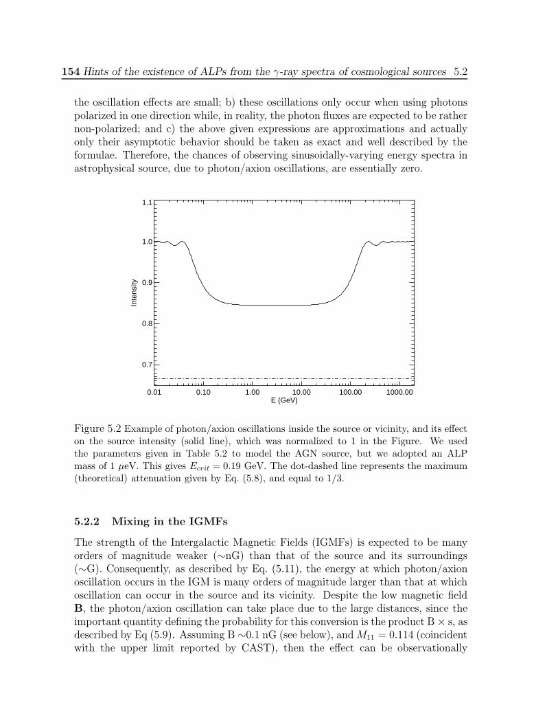
154 Hints of the existence of ALPs from the γ-ray spectra of cosmological sources 5.2
the oscillation effects are small; b) these oscillations only occur when using photonspolarized in one direction while, in reality, the photon fluxes are expected to be rathernon-polarized; and c) the above given expressions are approximations and actuallyonly their asymptotic behavior should be taken as exact and well described by theformulae. Therefore, the chances of observing sinusoidally-varying energy spectra inastrophysical source, due to photon/axion oscillations, are essentially zero.
0.01 0.10 1.00 10.00 100.00 1000.00E (GeV)
0.7
0.8
0.9
1.0
1.1
Inte
nsity
Figure 5.2 Example of photon/axion oscillations inside the source or vicinity, and its effecton the source intensity (solid line), which was normalized to 1 in the Figure. We usedthe parameters given in Table 5.2 to model the AGN source, but we adopted an ALPmass of 1 µeV. This gives Ecrit = 0.19 GeV. The dot-dashed line represents the maximum(theoretical) attenuation given by Eq. (5.8), and equal to 1/3.
5.2.2 Mixing in the IGMFs
The strength of the Intergalactic Magnetic Fields (IGMFs) is expected to be manyorders of magnitude weaker (∼nG) than that of the source and its surroundings(∼G). Consequently, as described by Eq. (5.11), the energy at which photon/axionoscillation occurs in the IGM is many orders of magnitude larger than that at whichoscillation can occur in the source and its vicinity. Despite the low magnetic fieldB, the photon/axion oscillation can take place due to the large distances, since theimportant quantity defining the probability for this conversion is the product B × s, asdescribed by Eq (5.9). Assuming B ∼0.1 nG (see below), and M11 = 0.114 (coincidentwith the upper limit reported by CAST), then the effect can be observationally
5.2 The formalism 155
detectable (Ecrit < 1 TeV) only if the ALP mass is ma < 6 × 10⁻¹⁰ eV. If the axionmass ma was larger than this value, then the consequences of this oscillation couldnot be probed with the current generation of IACTs, that observe up to few tens ofTeV 3. In our fiducial model (see Table 5.2) we used ma = 10−10 eV, which impliesEcrit = 28.5 GeV.
It is important to stress that at energies larger than 10 GeV, and especially largerthan 100 GeV, besides the oscillation to ALPs, the photons should also be affectedby the diffuse radiation from the Extragalactic Background Light (EBL). The EBLintroduces an attenuation in the photon flux due to e−e+ pair production that comesfrom the interaction of the gamma-ray source photons with infrared and optical-UVbackground photons for the energies under consideration (Hauser & Dwek 2001).Therefore, it will be necessary to modify the above equations to properly account forthe EBL in our calculations. These equations can be found in Csaki et al. (2003),where the photon/axion mixing in the IGMF was also studied, although for otherpurposes and a different energy range. We note that the same equations were alsoused in De Angelis et al. (2007) to study for the first time the photon/axion mixingin the presence of IGMFs for the same energy range that we are considering in thiswork.
There is little information on the strength and morphology of the IGMFs. As forthe morphology, several authors reported that space should be divided into severaldomains, each of them with a size for which the magnetic field is coherent. Differentdomains will have randomly changing directions of B field of about the same strength(Kronberg 1994, Furlanetto & Loeb 2001). The IGMF strength is constrained to besmaller than 1 nG (Grasso & Rubinstein 2001), which is somewhat supported by theestimates of ∼0.3-0.9 nG that can be inferred (De Angelis et al. 2008) from recentobservations of the Pierre Auger Observatory (Abraham et al. 2008). On the otherhand, there is controversy on the possibility of generating such a strong magneticfield. Detailed simulations yield IGMFs of the order of 0.01 nG so that they can laterreproduce the measured B fields in nearby galaxy clusters (Dolag et al. 2005, Siglet al. 2004). Given this controversy, we decided to use a mid-value of 0.1nG in ourfiducial model (Table 5.2).
In our model, we assume that the photon beam propagates over N domains ofa given length, the modulus of the magnetic field B roughly constant in each ofthem. We will take, however, randomly chosen orientations, which in practice willbe also equivalent to a variation in the strength of the component of the magneticfield involved in the photon/axion mixing. If the photon beam is propagating alongthe y axis, the oscillation will occur with magnetic fields in the x and z directionssince the polarization of the photon can only be along those axis. Therefore, we candescribe the beam state by the vector (γx, γz, a). The transfer equation will be (Csaki
3The next generation of IACTs (namely AGIS and CTA) aim for an order of magnitude ofimprovement at the highest energies, reaching few hundreds of TeV; but those instruments will notbe in operation till 2013 or later.

156 Hints of the existence of ALPs from the γ-ray spectra of cosmological sources 5.2
0 500 1000 1500 2000D (Mpc)
1
Inte
nsity
0 500 1000 1500 2000D (Mpc)
1
Inte
nsity
0 500 1000 1500 2000D (Mpc)
0.1
1.0
Inte
nsity
0 500 1000 1500 2000D (Mpc)
0.1
1.0
Inte
nsity
0 500 1000 1500 2000D (Mpc)
0.001
0.010
0.100
1.000
Inte
nsity
0 500 1000 1500 2000D (Mpc)
0.001
0.010
0.100
1.000
Inte
nsity
Figure 5.3 Effect of intergalactic photon/axion mixing on photon and ALP intensitiesversus distance to the source, computed for our fiducial model, i.e. for 3C 279 and thoseparameters given in Table 5.2 but taking B= 1 nG, and using the Primack EBL model.The black thick solid line represents the total photon intensity, while the blue dotted line isthe ALP intensity. The photon intensity as given only by the EBL (i.e. without includingphoton/axion mixing) is shown as the red dashed line. Left panels: mixing computed forM11 = 4 GeV and an initial photon energy of 50 GeV (top), 500 GeV (middle) and 2 TeV(bottom); right panels: M11 = 0.7 GeV and same energies than left panels.
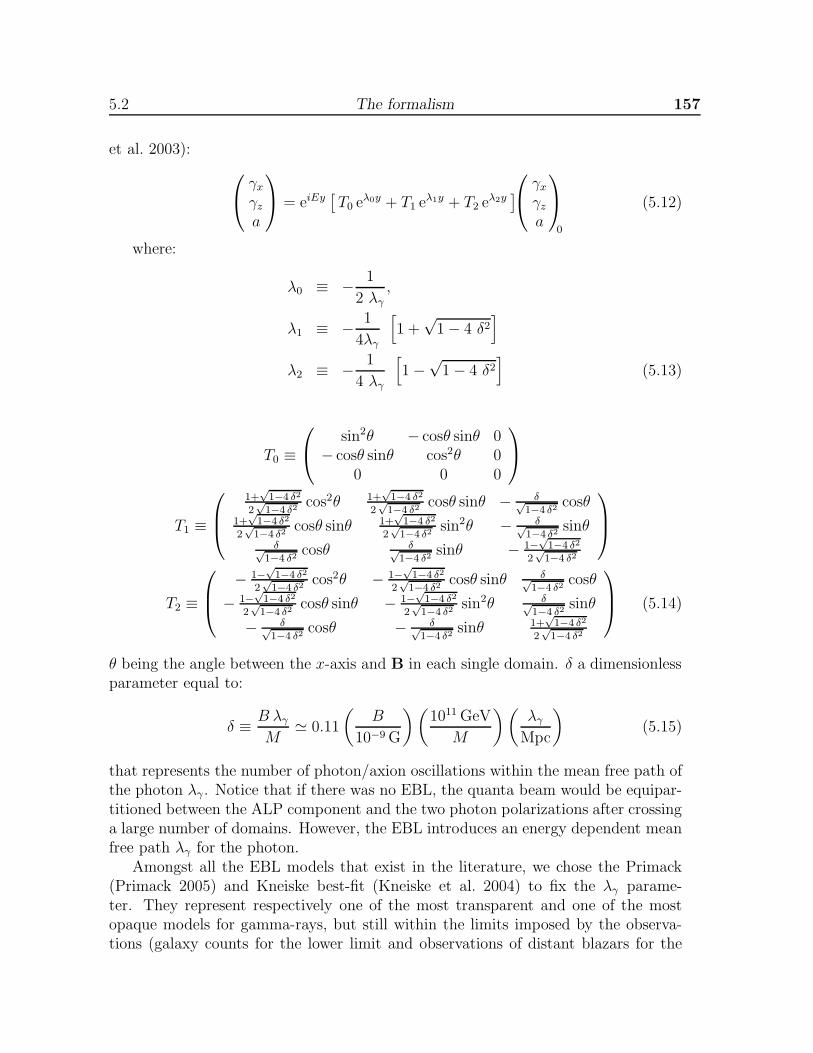
5.2 The formalism 157
et al. 2003):
γx
γz
a
= eiEy[
T0 eλ0y + T1 eλ1y + T2 eλ2y]
γx
γz
a
0
(5.12)
where:
λ0 ≡ − 1
2 λγ
,
λ1 ≡ − 1
4λγ
[
1 +√
1 − 4 δ2]
λ2 ≡ − 1
4 λγ
[
1 −√
1 − 4 δ2]
(5.13)
T0 ≡
sin2θ − cosθ sinθ 0− cosθ sinθ cos2θ 0
0 0 0
T1 ≡
1+√
1−4 δ2
2√
1−4 δ2 cos2θ 1+√
1−4 δ2
2√
1−4 δ2 cosθ sinθ − δ√1−4 δ2 cosθ
1+√
1−4 δ2
2√
1−4 δ2 cosθ sinθ 1+√
1−4 δ2
2√
1−4 δ2 sin2θ − δ√1−4 δ2 sinθ
δ√1−4 δ2 cosθ δ√
1−4 δ2 sinθ − 1−√
1−4 δ2
2√
1−4 δ2
T2 ≡
− 1−√
1−4 δ2
2√
1−4 δ2 cos2θ − 1−√
1−4 δ2
2√
1−4 δ2 cosθ sinθ δ√1−4 δ2 cosθ
− 1−√
1−4 δ2
2√
1−4 δ2 cosθ sinθ − 1−√
1−4 δ2
2√
1−4 δ2 sin2θ δ√1−4 δ2 sinθ
− δ√1−4 δ2 cosθ − δ√
1−4 δ2 sinθ 1+√
1−4 δ2
2√
1−4 δ2
(5.14)
θ being the angle between the x-axis and B in each single domain. δ a dimensionlessparameter equal to:
δ ≡ B λγ
M≃ 0.11
(
B
10−9 G
)(
1011 GeV
M
)(
λγ
Mpc
)
(5.15)
that represents the number of photon/axion oscillations within the mean free path ofthe photon λγ . Notice that if there was no EBL, the quanta beam would be equipar-titioned between the ALP component and the two photon polarizations after crossinga large number of domains. However, the EBL introduces an energy dependent meanfree path λγ for the photon.
Amongst all the EBL models that exist in the literature, we chose the Primack(Primack 2005) and Kneiske best-fit (Kneiske et al. 2004) to fix the λγ parame-ter. They represent respectively one of the most transparent and one of the mostopaque models for gamma-rays, but still within the limits imposed by the observa-tions (galaxy counts for the lower limit and observations of distant blazars for the
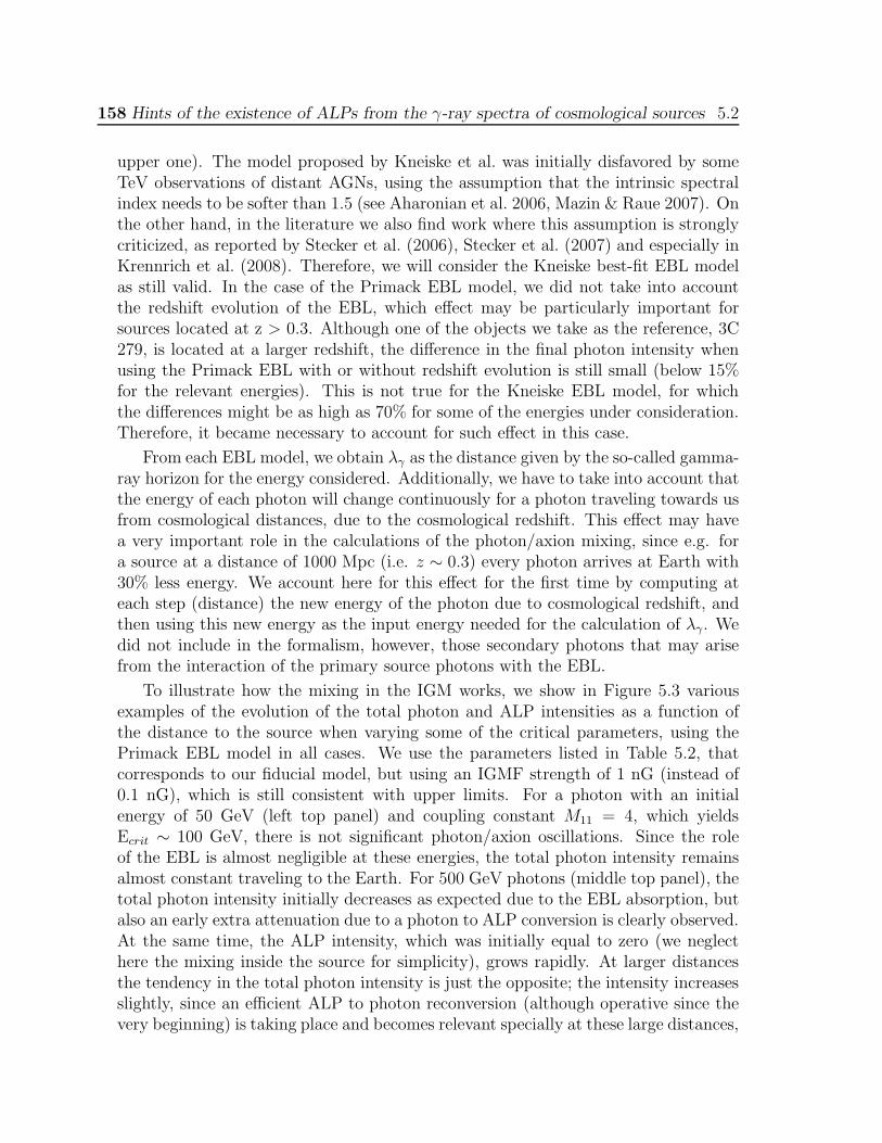
158 Hints of the existence of ALPs from the γ-ray spectra of cosmological sources 5.2
upper one). The model proposed by Kneiske et al. was initially disfavored by someTeV observations of distant AGNs, using the assumption that the intrinsic spectralindex needs to be softer than 1.5 (see Aharonian et al. 2006, Mazin & Raue 2007). Onthe other hand, in the literature we also find work where this assumption is stronglycriticized, as reported by Stecker et al. (2006), Stecker et al. (2007) and especially inKrennrich et al. (2008). Therefore, we will consider the Kneiske best-fit EBL modelas still valid. In the case of the Primack EBL model, we did not take into accountthe redshift evolution of the EBL, which effect may be particularly important forsources located at z > 0.3. Although one of the objects we take as the reference, 3C279, is located at a larger redshift, the difference in the final photon intensity whenusing the Primack EBL with or without redshift evolution is still small (below 15%for the relevant energies). This is not true for the Kneiske EBL model, for whichthe differences might be as high as 70% for some of the energies under consideration.Therefore, it became necessary to account for such effect in this case.
From each EBL model, we obtain λγ as the distance given by the so-called gamma-ray horizon for the energy considered. Additionally, we have to take into account thatthe energy of each photon will change continuously for a photon traveling towards usfrom cosmological distances, due to the cosmological redshift. This effect may havea very important role in the calculations of the photon/axion mixing, since e.g. fora source at a distance of 1000 Mpc (i.e. z ∼ 0.3) every photon arrives at Earth with30% less energy. We account here for this effect for the first time by computing ateach step (distance) the new energy of the photon due to cosmological redshift, andthen using this new energy as the input energy needed for the calculation of λγ. Wedid not include in the formalism, however, those secondary photons that may arisefrom the interaction of the primary source photons with the EBL.
To illustrate how the mixing in the IGM works, we show in Figure 5.3 variousexamples of the evolution of the total photon and ALP intensities as a function ofthe distance to the source when varying some of the critical parameters, using thePrimack EBL model in all cases. We use the parameters listed in Table 5.2, thatcorresponds to our fiducial model, but using an IGMF strength of 1 nG (instead of0.1 nG), which is still consistent with upper limits. For a photon with an initialenergy of 50 GeV (left top panel) and coupling constant M11 = 4, which yieldsEcrit ∼ 100 GeV, there is not significant photon/axion oscillations. Since the roleof the EBL is almost negligible at these energies, the total photon intensity remainsalmost constant traveling to the Earth. For 500 GeV photons (middle top panel), thetotal photon intensity initially decreases as expected due to the EBL absorption, butalso an early extra attenuation due to a photon to ALP conversion is clearly observed.At the same time, the ALP intensity, which was initially equal to zero (we neglecthere the mixing inside the source for simplicity), grows rapidly. At larger distancesthe tendency in the total photon intensity is just the opposite; the intensity increasesslightly, since an efficient ALP to photon reconversion (although operative since thevery beginning) is taking place and becomes relevant specially at these large distances,
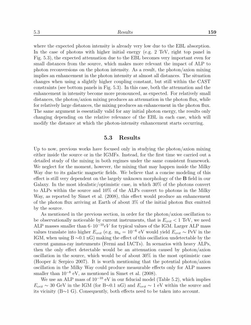
5.3 Results 159
where the expected photon intensity is already very low due to the EBL absorption.In the case of photons with higher initial energy (e.g. 2 TeV, right top panel inFig. 5.3), the expected attenuation due to the EBL becomes very important even forsmall distances from the source, which makes more relevant the impact of ALP tophoton reconversions on the photon intensity. As a result, the photon/axion mixingimplies an enhancement in the photon intensity at almost all distances. The situationchanges when using a slightly higher coupling constant, but still within the CASTconstraints (see bottom panels in Fig. 5.3). In this case, both the attenuation and theenhancement in intensity become more pronounced, as expected. For relatively smalldistances, the photon/axion mixing produces an attenuation in the photon flux, whilefor relatively large distances, the mixing produces an enhancement in the photon flux.The same argument is essentially valid for any initial photon energy, the results onlychanging depending on the relative relevance of the EBL in each case, which willmodify the distance at which the photon-intensity enhancement starts occurring.
5.3 Results
Up to now, previous works have focused only in studying the photon/axion mixingeither inside the source or in the IGMFs. Instead, for the first time we carried out adetailed study of the mixing in both regimes under the same consistent framework.We neglect for the moment, however, the mixing that may happen inside the MilkyWay due to its galactic magnetic fields. We believe that a concise modeling of thiseffect is still very dependent on the largely unknown morphology of the B field in ourGalaxy. In the most idealistic/optimistic case, in which 30% of the photons convertto ALPs within the source and 10% of the ALPs convert to photons in the MilkyWay, as reported by Simet et al. (2008), this effect would produce an enhancementof the photon flux arriving at Earth of about 3% of the initial photon flux emittedby the source.
As mentioned in the previous section, in order for the photon/axion oscillation tobe observationally noticeable by current instruments, that is Ecrit < 1 TeV, we needALP masses smaller than 6 ·10−10eV for typical values of the IGM. Larger ALP massvalues translate into higher Ecrit (e.g. ma = 10−6 eV would yield Ecrit ∼ PeV in theIGM, when using B ∼0.1 nG) making the effect of this oscillation undetectable by thecurrent gamma-ray instruments (Fermi and IACTs). In scenarios with heavy ALPs,then the only effect detectable would be an attenuation caused by photon/axionoscillation in the source, which would be of about 30% in the most optimistic case(Hooper & Serpico 2007). It is worth mentioning that the potential photon/axionoscillation in the Milky Way could produce measurable effects only for ALP massessmaller than 10−8 eV, as mentioned in Simet et al. (2008).
We use an ALP mass of 10−10 eV in our fiducial model (Table 5.2), which impliesEcrit ∼ 30 GeV in the IGM (for B∼0.1 nG) and Ecrit ∼ 1 eV within the source andits vicinity (B∼1 G). Consequently, both effects need to be taken into account.

160 Hints of the existence of ALPs from the γ-ray spectra of cosmological sources 5.3
5.3.1 Photon/axion oscillation in our framework
In this section we show the results obtained when taking into account the mixinginside the source and in the IGMF simultaneously. Since we expect the intergalacticmixing to be more important for larger distances, due to the more prominent roleof the EBL, we chose two distant astrophysical sources (as our benchmark AGNs)that are relatively well characterized at gamma-ray energies; namely the radio quasar3C 279 (z=0.536), most distant detected gamma-ray source at the VHE range, and theBL Lac PKS 2155-304 at z=0.117. In order to compute the photon/axion oscillationin the source we used the parameters reported in Hartmann et al. (2001) for 3C 279and Kusunose & Takahara (2008) for PKS 2155-304. As for the size of the region withB field (where photons can convert to ALPs) we chose a region 10 times larger thanthe radius of the gamma-ray emitting blob given in the above mentioned references,the reason being that the blob radius represents only a lower limit for the regionwhere B is confined. We note that this parameter, as well as the number of domainswhere the B is coherent, play an important role in the photon attenuations due tothe photon/axion mixing in the source. Table 5.1 shows the different attenuationsthat are obtained when varying the size of the region where B is confined (what wecalled “B region”) and the lengths of coherent B domains inside that region. Onecan see that, once the number of domains is fixed, the photon attenuation increaseswhen increasing the size of the “B region”. On the other hand, when fixing the sizeof the “B region” and scanning the size of the domains we find that, as we increasethe number of domains, the attenuation increases until the size of the domain is “toosmall”. At this point, the probability of photon/axion conversion is almost zero forthe single domains, which reduces the overall photon/axion conversion.
Table 5.1 Maximum attenuations due to photon/axion oscillations in the source obtainedfor different sizes of the region where the magnetic field is confined (“B region”) and differentlengths for the coherent domains. Only length domains smaller than the size of the B regionare possible. The B field strength used is 1.5 G (see Table 5.2). The photon flux intensitywithout ALPs was normalized to 1. In bold face, is the attenuation given by our fiducialmodel.
B region (pc) Length domains (pc)3×10⁻⁴ 3×10⁻³ 0.03 0.3
0.3 0.84 0.67 0.67 0.750.03 0.98 0.84 0.77 -
3×10⁻³ 0.99 0.98 - -
We summarize in Table 5.2 the parameters we have considered in order to calculatethe total photon/axion conversion in both the source (for the two benchmark AGNs)and in the IGM. As we already mentioned, these values represent our fiducial model.

5.3 Results 161
Table 5.2 Parameters used to calculate the total photon/axion conversion in both thesource (for the two AGNs considered, 3c279 and PKS 2155-304) and in the IGM. Thevalues related to 3C 279 were obtained from Hartmann et al. (2001), while those ones forPKS 2155-304 were obtained from Kusunose & Takahara (2008). As for the IGM, ed,int
was obtained from Peebles (1993), and Bint was chosen to be well below the upper limittypically given in the literature (see discussion in the text). This Table represents ourfiducial model.
Parameter 3C 279 PKS 2155-304B (G) 1.5 0.1
Source ed (cm−3) 25 160parameters L domains (pc) 0.003 3 × 10⁻⁴
B region (pc) 0.03 0.003z 0.536 0.117
Intergalactic ed,int (cm−3) 10−7 10−7
parameters Bint (nG) 0.1 0.1L domains (Mpc) 1 1
ALP M (GeV) 1.14 × 10¹⁰ 1.14 × 10¹⁰
parameters ALP mass (eV) 10−10 10−10
The effect of existence of ALPs on the total photon flux coming from 3C 279 andfrom PKS 2155-304 (using the fiducial model presented in Table 5.2) can be seenin Figure 5.4. We carried out the calculations for the two EBL models cited above:Kneiske best-fit and Primack. The inferred critical energies for the mixing in thesource are Ecrit = 4.6 eV for 3C 279 and Ecrit = 69 eV for PKS 2155-304, while forthe mixing in the IGM we obtain Ecrit = 28.5 GeV. The photon attenuation due tophoton/axion mixing inside the source is 16% for 3C 279 and 1% for PKS 2155-304,as can be seen above their respective critical energies in Figure 5.4. On the otherhand, the photon attenuation due to photon/axion oscillation in the IGM is 30% forthe distance of both sources, and it occurs at the same critical energy. The role ofthe EBL is negligible at this low energy (i.e. below ∼100 GeV), which means thatthe intensity curves for the two EBL models agree to this energy.
The situation changes above ∼100 GeV, where the photon attenuation due tothe EBL is noticeable. At this point, the results depend substantially on the sourcedistance and the EBL model used. A stronger photon attenuation is obtained for theKneiske best-fit model against the Primack EBL model, as expected. Because thestrong photon attenuation due to the EBL, the ALPs that later convert to photonsimply a further enhancement of the expected photon flux. Therefore, as one cannotice from Figure 5.4, the existence of ALPs translates into a relatively small (∼30%)intensity attenuation at low energies and a large intensity enhancement (several ordersof magnitude, depending on the energy range, distance of the source and chosen EBL

162 Hints of the existence of ALPs from the γ-ray spectra of cosmological sources 5.3
0.1 1.0 10.0 100.0 1000.0E (GeV)
10-6
10-5
10-4
10-3
10-2
10-1
100
Inte
nsity
0.1 1.0 10.0 100.0 1000.0 10000.0E (GeV)
0.01
0.10
1.00
Inte
nsity
Figure 5.4 Effect of photon/axion conversions both inside the source and in the IGM onthe total photon flux coming from 3C 279 (z=0.536) and PKS 2155-304 (z=0.117) for twoEBL models: Kneiske best-fit (dashed line) and Primack (solid line). The expected photonflux without including ALPs is also shown for comparison (dotted line for Kneiske best-fitand dot-dashed line for Primack).
model) at high energies.
In order to quantitatively study the effect of ALPs on the total photon intensity,we plot in Figure 5.5 the difference between the predicted arriving photon intensitywithout including ALPs and that one obtained when including the photon/axionoscillations (called here the axion boost factor). Again, this was done for our fiducialmodel (Table 5.2) and for the two EBL models described above. The plots showdifferences in the axion boost factors obtained for 3C 279 and PKS 2155-304 due
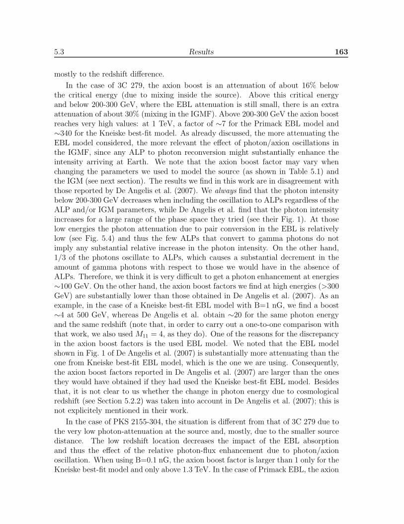
5.3 Results 163
mostly to the redshift difference.
In the case of 3C 279, the axion boost is an attenuation of about 16% belowthe critical energy (due to mixing inside the source). Above this critical energyand below 200-300 GeV, where the EBL attenuation is still small, there is an extraattenuation of about 30% (mixing in the IGMF). Above 200-300 GeV the axion boostreaches very high values: at 1 TeV, a factor of ∼7 for the Primack EBL model and∼340 for the Kneiske best-fit model. As already discussed, the more attenuating theEBL model considered, the more relevant the effect of photon/axion oscillations inthe IGMF, since any ALP to photon reconversion might substantially enhance theintensity arriving at Earth. We note that the axion boost factor may vary whenchanging the parameters we used to model the source (as shown in Table 5.1) andthe IGM (see next section). The results we find in this work are in disagreement withthose reported by De Angelis et al. (2007). We always find that the photon intensitybelow 200-300 GeV decreases when including the oscillation to ALPs regardless of theALP and/or IGM parameters, while De Angelis et al. find that the photon intensityincreases for a large range of the phase space they tried (see their Fig. 1). At thoselow energies the photon attenuation due to pair conversion in the EBL is relativelylow (see Fig. 5.4) and thus the few ALPs that convert to gamma photons do notimply any substantial relative increase in the photon intensity. On the other hand,1/3 of the photons oscillate to ALPs, which causes a substantial decrement in theamount of gamma photons with respect to those we would have in the absence ofALPs. Therefore, we think it is very difficult to get a photon enhancement at energies∼100 GeV. On the other hand, the axion boost factors we find at high energies (>300GeV) are substantially lower than those obtained in De Angelis et al. (2007). As anexample, in the case of a Kneiske best-fit EBL model with B=1 nG, we find a boost∼4 at 500 GeV, whereas De Angelis et al. obtain ∼20 for the same photon energyand the same redshift (note that, in order to carry out a one-to-one comparison withthat work, we also used M11 = 4, as they do). One of the reasons for the discrepancyin the axion boost factors is the used EBL model. We noted that the EBL modelshown in Fig. 1 of De Angelis et al. (2007) is substantially more attenuating than theone from Kneiske best-fit EBL model, which is the one we are using. Consequently,the axion boost factors reported in De Angelis et al. (2007) are larger than the onesthey would have obtained if they had used the Kneiske best-fit EBL model. Besidesthat, it is not clear to us whether the change in photon energy due to cosmologicalredshift (see Section 5.2.2) was taken into account in De Angelis et al. (2007); this isnot explicitely mentioned in their work.
In the case of PKS 2155-304, the situation is different from that of 3C 279 due tothe very low photon-attenuation at the source and, mostly, due to the smaller sourcedistance. The low redshift location decreases the impact of the EBL absorptionand thus the effect of the relative photon-flux enhancement due to photon/axionoscillation. When using B=0.1 nG, the axion boost factor is larger than 1 only for theKneiske best-fit model and only above 1.3 TeV. In the case of Primack EBL, the axion
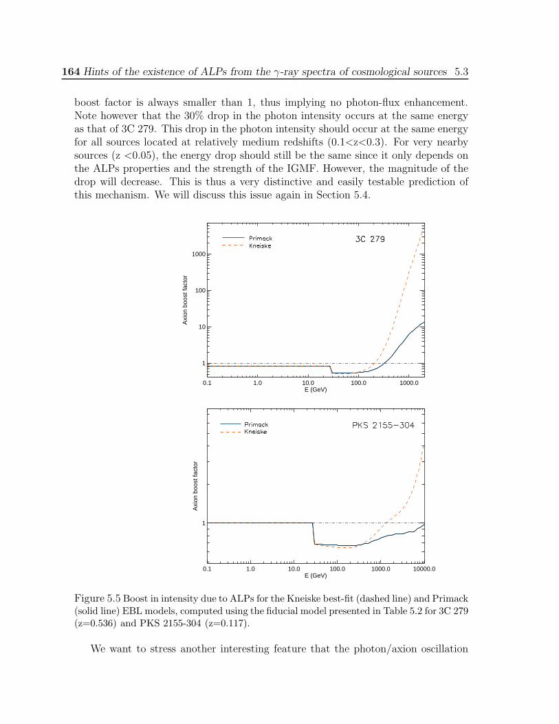
164 Hints of the existence of ALPs from the γ-ray spectra of cosmological sources 5.3
boost factor is always smaller than 1, thus implying no photon-flux enhancement.Note however that the 30% drop in the photon intensity occurs at the same energyas that of 3C 279. This drop in the photon intensity should occur at the same energyfor all sources located at relatively medium redshifts (0.1<z<0.3). For very nearbysources (z <0.05), the energy drop should still be the same since it only depends onthe ALPs properties and the strength of the IGMF. However, the magnitude of thedrop will decrease. This is thus a very distinctive and easily testable prediction ofthis mechanism. We will discuss this issue again in Section 5.4.
0.1 1.0 10.0 100.0 1000.0E (GeV)
1
10
100
1000
Axi
on b
oost
fact
or
0.1 1.0 10.0 100.0 1000.0 10000.0E (GeV)
1
Axi
on b
oost
fact
or
Figure 5.5 Boost in intensity due to ALPs for the Kneiske best-fit (dashed line) and Primack(solid line) EBL models, computed using the fiducial model presented in Table 5.2 for 3C 279(z=0.536) and PKS 2155-304 (z=0.117).
We want to stress another interesting feature that the photon/axion oscillation

5.3 Results 165
in the IGMF produces in the source spectra at VHE (>100 GeV) of distant sources(z>0.1). As one can notice from Fig. 5.5, the axion boost factor starts increasingat few hundred GeV (when the EBL becomes important), and consequently it willmake the source spectra to look harder than they are actually. This happens forboth AGNs, yet at slightly different energies: 100 GeV for 3C 279 and 300 GeV forPKS 2155-304. As shown in Figure. 5.5, the hardening of the VHE spectra occurs forboth (very different) EBL models that we used, and hence a very robust predictionof this mechanism being at work. Such a hardening of the spectra was alreadypredicted in Simet et al. (2008) for several AGNs located at redshifts 0.1-0.2. Whilein our work the effect is due mostly to the photon/axion oscillation in the IGMF,in Simet et al. (2008) the effect is due to photon/axion oscillation within the source(up to 30% attenuation of the photon flux) and the one that occurs in the galacticmagnetic fields of the Milky Way (up to 10% conversion probability). It is worthmentioning here, however, that when using the parameters (essentially B strengthand size of the “B region”) for the modeling of the gamma-ray emission from AGNsources, we find that the attenuation in the source due to photon/axion conversionis relatively low; 16% for our model of 3C 279 and 1% for that of PKS 2155-304.These low photon-flux attenuation (equivalent to ALP-enhancement) would decreasesignificantly the effect of the mechanism proposed in Simet et al. (2008).
Finally, it is worth mentioning that we checked that our results are robust againstthe randomness of the B field. We ran 100 different realizations of the same physicalscenario, randomly varying the orientation of B in each coherent domain and eachrealization. We did so for the four cases studied along this work, i.e. 3C 279 and PKS2155-304, Primack and Kneiske best-fit EBL models. Furthermore, we repeated thesame exercise using 0.1, 1 and 10 Mpc as the length of the coherent domains in orderto explore the dependence of our results on this parameter. In all cases, we choseour fiducial value of 0.1 nG for the B field strength. We found that the maximumdifferences are typically well below 10%, implying that the results obtained are notsensitive to the randomness of the B field. We increased the number of realizationsto 1000 for some cases and found no differences with respect to the results obtainedwith 100 realizations.
A larger effect on the computed axion-boost factors occurs when changing thesize of the domains being used. The computed axion-boost factors are sensitive tochoice of the size of the coherent domains to be used. Together with the choice ofthe EBL model (which is also uncertain), the choice of the domain sizes modifies theresults obtained by factors of a few.
5.3.2 The impact of changing B
A very interesting result has been found when varying the modulus of the intergalacticmagnetic field. In Simet et al. (2008), the intergalactic photon/axion mixing wasrejected arguing that its effect on the final intensity at Earth would be negligible
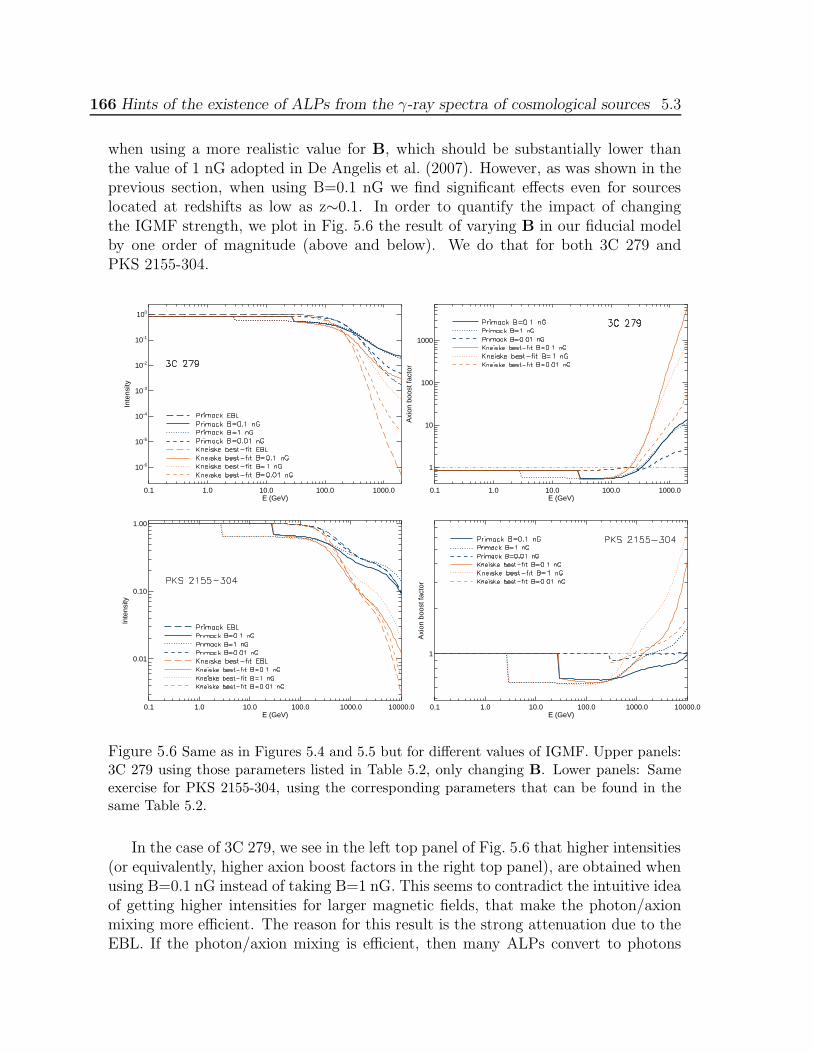
166 Hints of the existence of ALPs from the γ-ray spectra of cosmological sources 5.3
when using a more realistic value for B, which should be substantially lower thanthe value of 1 nG adopted in De Angelis et al. (2007). However, as was shown in theprevious section, when using B=0.1 nG we find significant effects even for sourceslocated at redshifts as low as z∼0.1. In order to quantify the impact of changingthe IGMF strength, we plot in Fig. 5.6 the result of varying B in our fiducial modelby one order of magnitude (above and below). We do that for both 3C 279 andPKS 2155-304.
0.1 1.0 10.0 100.0 1000.0E (GeV)
10-6
10-5
10-4
10-3
10-2
10-1
100
Inte
nsity
0.1 1.0 10.0 100.0 1000.0E (GeV)
1
10
100
1000
Axi
on b
oost
fact
or
0.1 1.0 10.0 100.0 1000.0 10000.0E (GeV)
0.01
0.10
1.00
Inte
nsity
0.1 1.0 10.0 100.0 1000.0 10000.0E (GeV)
1
Axi
on b
oost
fact
or
Figure 5.6 Same as in Figures 5.4 and 5.5 but for different values of IGMF. Upper panels:3C 279 using those parameters listed in Table 5.2, only changing B. Lower panels: Sameexercise for PKS 2155-304, using the corresponding parameters that can be found in thesame Table 5.2.
In the case of 3C 279, we see in the left top panel of Fig. 5.6 that higher intensities(or equivalently, higher axion boost factors in the right top panel), are obtained whenusing B=0.1 nG instead of taking B=1 nG. This seems to contradict the intuitive ideaof getting higher intensities for larger magnetic fields, that make the photon/axionmixing more efficient. The reason for this result is the strong attenuation due to theEBL. If the photon/axion mixing is efficient, then many ALPs convert to photons

5.3 Results 167
which soon disappear due to the EBL absorption. Consequently, if the source distanceis large, we end up having a very small number of photons arriving to the Earth. Onthe other hand, if the photon/axion mixing is not that strong, then we can keep ahigher number of ALPs traveling towards the Earth, which act as a potential reservoirof photons. When decreasing B to 0.01 nG, then the axion boost factors are lowerthan for the other two cases. On the other hand, in the case of PKS 2155-304, we seethat the highest axion boost factors are obtained with B=1 nG, because the sourceis not as distant as 3C 279. If we had considered a source located at a much furtherdistance than 3C 279, then we would have found the highest axion boost factors forB=0.01 nG.
In summary, higher B values do not necessarily translate into higher photon fluxenhancements. There is always a B value that maximizes the axion boost factors;this value is sensitive to the source distance, the considered energy and the EBLadopted model.
5.3.3 The impact of using the smallest photon/ALP coupling constant
The most stringent limits on the ALP-photon coupling constant were derived us-ing the non-detection of gamma-rays (by the Solar Maximum Mission Gamma-RaySpectrometer) from the supernova (SN) 1987A during the ∼10 seconds time windowdefined by the neutrino burst. This outstanding event allowed several authors in 1996to set lower limits to the inverse of the coupling constant M11 to values larger than1 (Brockway et al. 1996) and 3 (Griffols et al. 1996). Those limits are only valid forultralight ALPs. In both works the value ma < 10−9 eV is quoted, although this valueholds only for some specific situations. Indeed, a more robust value is ma < 10−11
eV (see Hooper & Serpico 2007, Simet et al. 2008), i.e. the energy below which theexact value of the ALP mass is irrelevant because the “plasma frequency” dominates(see definition of ALP effective mass in Section 5.2.1). Various authors (see Csaki etal. 2003), De Angelis et al. 2007) used M11 = 4 when dealing with ma < 1010 eV.Since the ALP mass in our fiducial model is 10−10 eV, and hence close to this limit,we decided to repeat the calculations using this value for M , which is 35 times largerthan the value we used in the previous sections (see Table 5.2).
Before we continue, it is worth pointing out that the limits to the ALP-photoncoupling constant given in Brockway et al. (1996) and Griffols et al. (1996) are subjectto large uncertainties that are not fully discussed in those papers. Both the flux ofALPs produced in the SN explosion and the back-conversion of ALPs to gammaphotons can vary by large factors, and hence the upper limits computed with thosenumbers have to be taken with caveats.
The calculated flux of ALPs produced and released during the SN explosion de-pends on the knowledge of the size, temperature and density of the proto-neutronstar. Those numbers are subject to large uncertainties because we still do not knowhow stars explode. Even though there is general agreement that the ultimate energy

168 Hints of the existence of ALPs from the γ-ray spectra of cosmological sources 5.4
source is gravity, the relative roles of neutrinos, fluid instabilities, rotation and mag-netic fields continue to be debated. In particular, back in the 90s it was believedthat neutrinos would be able to reheat the outgoing shock-wave and produce theexplosion. Nowadays, with far more powerful computer simulations, we know thatneutrino-driven explosions are only possible when the star has a small iron core andlow density in the surrounding shells, as being found in stars near or below 10 solarmasses (Janka et al. 2007). The progenitor of SN1987A was a blue supergiant andhence it is expected to be somewhere between 10-50 solar masses. A possibility toexplain those explosions might require the proper inclusion of rotation and magneticfields (see Burrows et al. 2007, Obergaulinger et al. 2008, Dimmelmeier et al. 2008and references therein). Both B field and rotation are present in stars as well as inpulsars, which are the products of successful SN explosions; thus it is very naturalto consider them in SN explosion models. In particular, the rotation of the proto-neutron star can change substantially the temperature and, specially, the density ofthe inner core; in Dimmelmeier et al. (2008) it is shown that the density can varyby more than one order of magnitude, which would change by a similar factor theflux of ALPs being produced. Brockway et al. (1996) and Griffols et al. (1996) didnot consider such level of complexity (and uncertainties) in the parameters used tocompute the flux of ALPs, mostly because 15 years ago we lacked that knowledge.
On the other hand, the back-conversion of ALPs to photons relies on the structureof the galactic magnetic field which is, again, not well known. Different models predictB fields that could differ substantially and hence they would predict different valuesfor the amount of gamma photons we would obtain for a given flux of ALPs. Thisis clearly shown in Fig. 1 from Simet et al. (2008), where the probability of ALP-photon conversion is given for various locations of the sky. Therefore, even if wecould accurately predict the number of ALPs from SN1987A, the number of photonswould be subject to large uncertainties.
Therefore, we conclude that the limit in the inverse of the ALP-photon couplingconstant given in Brockway et al. (1996) and Griffols et al. (1996) is subject tolarge (orders of magnitude) uncertainties, and thus the limit given by the CASTcollaboration remains as the most robust one up to date. However, for the sakeof comparison with other works, we computed the axion-boost factors when usingM11 = 4 eV. This is shown in Figure 5.7 for both 3C 279 and PKS 2155-304 for twovalues of the B field, 0.1 nG and 1 nG. For this low coupling constant, the effect due tothe photon/ALP oscillation in the source is negligible. The effect due to photon/ALPoscillation in the IGMF in not negligible, but substantially lower than the one shownin the previous section. Besides, such effect shows up at larger energies now (see Eq.5.11); 100 GeV and 1000 GeV respectively for 1 nG and 0.1 nG.

5.4 Detection prospects for Fermi and IACTs 169
0.1 1.0 10.0 100.0 1000.0E (GeV)
1
10
100
1000
Axi
on b
oost
fact
or
0.1 1.0 10.0 100.0 1000.0 10000.0E (GeV)
1
Axi
on b
oost
fact
or
Figure 5.7 Boost in intensity due to ALPs for the Kneiske best-fit and Primack EBLmodels, computed using the fiducial model presented in Table 5.2 for 3C 279 (z=0.536) andPKS 2155-304 (z=0.117), but with M11 = 4 GeV and B=0.1 nG (dashed and solid linesfor Kneiske best-fit and Primack EBL models respectively) and B=1 nG (dot-dashed anddotted lines).
5.4 Detection prospects for Fermi and IACTs
As mentioned in Section 5.2, for photon/axion coupling constants close to the cur-rent published limits, and for realistic ALP mass values, the energy at which thephoton/axion oscillation starts to become important is expected to lie in the gamma-ray range. Consequently, the combination of the Fermi/LAT instrument and theIACTs, which cover 6 decades in energy (from 20 MeV to 20 TeV) is very well suited
170 Hints of the existence of ALPs from the γ-ray spectra of cosmological sources 5.4
to study the photon/axion mixing effect. Because of the rapid change in the predictedphoton intensity attenuation close to Ecrit, the energy resolution of the instrumentis very relevant in order to detect the ALP signatures. The Fermi/LAT instrumenthas an energy resolution of about 10%, whereas IACTs, above 150 GeV, have anenergy resolution of about 20-25%. The photon intensity attenuation we found inthis work goes from 0 to 30% due to the mixing in the source, plus essentially 30%due to the mixing in the IGM. This implies that one needs to be able to determinephoton fluxes with a precision better than 10%. Such level of precision might not beachievable for energies >10 GeV with Fermi, or for energies >1 TeV with IACTs dueto a low photon counting (which depends obviously on the brightness and hardness ofthe gamma-ray sources). On the other hand, if the source is emitting at ∼TeV ener-gies and is located at large distances, the photon/axion oscillation in the IGM couldtranslate into an intensity enhancement of more than one order of magnitude (seeFigures 5.4, 5.5, 5.6), which should be certainly easy to detect with current IACTs.
Therefore, if we accurately knew the intrinsic spectrum of the sources and/or thedensity of the EBL, we should be able to observationally detect ALP signatures for awide range of the parameter space (photon/axion coupling constant and ALP mass).The main problem is that we do neither know accurately the intrinsic spectrum of thesources nor the EBL density. Thus the potential detection of those ALP signaturesbecome quite challenging, but not impossible. In order to study this scenario, wepropose the following strategy:
1. Observe several AGNs located at different redshifts, as well as the same AGNundergoing different flaring states (low/high fluxes), at different energy ranges,from radio to TeV. This is important because the modeling of the gamma-rayemission depends critically on the emission at lower energies (specially infrared,optical, UV and X-rays), and also because we do not know a priori the energyat which the photon/axion oscillation will start to operate.
2. Try to describe the observational data with “conventional” theoretical mod-els for the broad band emission (Synchrotron Self-Compton, External Comp-ton, Proton synchrotron, etc) and the attenuation of the gamma-rays in theEBL (Primack, Kneiske best-fit or other EBL models). The current models(sometimes very simplistic) will definitely require some modifications to fit theobservational data.
3. Look for intensity drops in the residuals (“best-model”-data). We want to stressthat the drop in the photon flux due to the attenuation in the IGM only dependson the IGMF and the properties of the ALPs (mass and coupling constant),i.e. it is independent of the gamma-ray sources. Therefore, a detection of suchphoton flux drops at the same energy in a numerous of different sources wouldbe a clear signature for the existence of photon/axion oscillation, because wedo not expect that the intrinsic spectrum from different sources (or same source
5.4 Detection prospects for Fermi and IACTs 171
at different flux levels) have a rapid drop of ∼30% in the emission at the sameenergy. The detection (or no-detection) of this photon intensity drop impliesa constraint for the product m2
a ·M11. In this specific search, the Fermi-LATinstrument is expected to play a key role since it will detect thousands of AGNsources located at various redshifts (up to z∼5), and at energies where thephoton absorption due to the EBL is not important.
4. Look for intensity enhancements in the residuals (i.e. “best-model”-data). Thisshould occur at the highest energies (E>300 GeV) and thus only detectablewith IACTs. The origin of the potential photon flux “excess” might be due toa wrong EBL model and/or wrong model for the source emission, the last beingvery important because it introduces differences between the different sources(or the same source under different activity levels). In this case what we needis to detect distant (z > 0.2) sources at the highest possible energies (>1 TeV).The current EBL models are already very close to the minimum possible photondensity limits from galaxy counts; that is, we cannot make them much moretransparent. That implies that the detection of TeV photons from a sourcethat is at redshift 0.5 (like 3C 279) could not be explained with conventionalphysics, regardless of the intrinsic spectrum of the source. This would be astrong hint for the existence of photon/axion oscillation. If the same effect wasobserved for different sources at different redshifts, we could try to parameterizethe effect by varying the ALP parameters (and/or the IGMF strength). If thatparameterization could be done successfully, then we would not only have avery strong hint for the existence of ALPs, but also would be able to constrainthe available parameter space (coupling constant and ALP mass).
The detection of ALPs is not trivial (and cannot be done with just few sources),but it is certainly possible, as we have shown above. Along these lines, it is worthmentioning that we might be already starting to see hints of the existence of ALPsfrom the gamma-ray spectra of cosmological sources. Very recent works already posesubstantial challenges to the conventional interpretation of the observed source spec-tra from several distant AGN sources. On the one hand, the VERITAS Collabora-tion recently claimed a detection of gamma-rays above 0.1 TeV (the highest detectedenergies are not yet reported) coming from 3C 66A (Acciari 2009), an intermediate-frequency-peaked BL Lac object located at redshift 0.444. This claim coincides withthe detection, at GeV energies, of this source in active state by the Fermi-LAT in-strument during the same time window (Tosti et al. 2008). In addition, the MAGICCollaboration reported gamma-rays above 1 TeV coming from a location consistentwith the position of 3C 66A (Aliu et al. 2009). Those observations would confirm theearlier claims from the Crimean Astrophysical ObservatoryOs GT-48 IACT of severaldetections from this source above 0.9 TeV (Nesphor et al. 1998, Stepaan et al. 2002).Those detections were not confirmed by the HEGRA and Whipple telescopes, which
172 Hints of the existence of ALPs from the γ-ray spectra of cosmological sources 5.5
are more sensitive instruments, but which observed the source at different time win-dows (Aharonian et al. 2000, Horan et al. 2004). As mentioned above, a detectionof TeV photons from a source located at z=0.444 would pose serious problems toconventional models of photon propagation over cosmological distances, where thehigh energy gammas are expected to disappear due to pair electron-positron pro-duction in the EBL. On the other hand, the recent published lower limits to theEBL at 3.6 microns (Levenson & Wright 2008), which is almost twice larger as theprevious ones, enhances even further the attenuation of gamma-rays at TeV energiesand thus increases even more the magnitude of the mystery. Furthermore, as re-ported in Krennrich et al. 2008, this fact extends the problems to sources located atmedium redshifts (z=0.1-0.2) whose intrinsic energy spectra appear to be harder thanpreviously anticipated. Those observations present blazar emission models with thechallenge of producing extremely hard intrinsic spectra (differential spectral index inthe spectrum smaller than 1.5) in the sub-TeV to multi-TeV regime. As mentioned inthe previous section, the photon/axion oscillation in the IGM would naturally explainthese two puzzles; the detection of TeV photons from very distant (z∼0.5) AGNs,and the apparent hardening of the spectra for relatively distant (z>0.1) AGNs.
However, it is worth mentioning that the above reported puzzles might still beexplained with conventional physics, as well as uncertainties in the published num-bers. The measured redshift of 3C 66A could be wrong (Bramel et al. 2005, Finkeet al. 2008), or the TeV photons reported by MAGIC could come from a neighbor-ing source (a radio galaxy), 3C 66B, which has never been detected in gamma-rays(Aliu et al. 2009). As for the blazars with intrinsic spectra harder than 1.5, thereis currently quite some controversy. Some authors claim that spectra harder than1.5 could be possible (see e.g. Katar et al. 2006, Stecker et al. 2007, Aharonian etal. 2008, Boettcher et al. 2008), while others state that spectra should be always softerthan 1.5 (see for instance Malkov & Drury 2001, Aharonian et al. 2006, Boettcher etal. 2008, Albert et al. 2008), and use this value to set upper limits to the EBL densityat infrared frequencies (Coppi & Aharonian 1999, Aharonian et al. 2006, Mazin &Raue 2007, Albert et al. 2008). An argument in favor of the latter is the fact thatEGRET never measured spectra harder than 1.5 at energies below 10 GeV, wherethe EBL does not distort the gamma-ray spectra, for any of the almost 100 detectedAGNs 4.
Finally, we would like to note that the capabilities of detecting the mentionedsignatures will increase significantly with the new generation of ground instruments,i.e. MAGIC II or HESS II (with lower energy thresholds, expected to operate in2009), CTA and AGIS (with even lower energy thresholds and higher sensitivity atmulti-TeV energies) and HAWC (higher sensitivity at multi-TeV energies, large dutycycles).
4In this matter, the Fermi-LAT instrument, with a sensitivity one order of magnitude better,and scanning the complete sky every 3 hours, is expected to see thousands of AGNs; which willsurely shed some light into this mystery.
5.5 Conclusions 173
5.5 Conclusions
If ALPs exist, then we should expect photon to ALP conversions (and vice-versa) inthe presence of magnetic fields. This photon/axion mixing will occur in gamma-raysources as well as in the IGM. We have explored in detail both mixing scenarios to-gether in the same framework. The main conclusions on this work can be summarizedas follows:
• If photons oscillate into ALPs in the IGM, then photon/axion mixing in thesource is also at work for lower photon energies. In this picture, both effectsshould be taken into account using the same framework, since they will begoverned by the same set of physical parameters (ALP mass and coupling con-stant). In the case of ALP masses ma >> 10−10 eV, the energies at which thephoton/axion oscillation occur in the IGMF are >> 1 TeV and thus not de-tectable with current gamma-ray instruments. In those cases the photon/axionoscillation in the source would be the only effect that could potentially be de-tected.
• The photon/axion oscillation in the source (and its vicinity) can produce photon-flux attenuations up to 30%, as previously stated in the literature (Hooper &Serpico 2007, Simet et al. 2008). However, when using available models forgamma-ray emitting blob regions to set values of the B field strength and thesize of the region where the conversion can take place (we took a radius 10 timesthe size of the blob), we obtain photon-flux attenuations that are significantlylower.
• The photon/axion oscillation in the IGM produces a photon-flux attenuationup to 30% below the energies at which the EBL is important (but above Ecrit
for the oscillation to be efficient). If the source redshift is larger than ∼0.1,this drop in intensity should be about 30% and it shows up in all sources atthe same energy. Hence, it presents relatively easy signature of the presenceof ALPs. The Fermi-LAT instrument is expected to play a very importantrole in this search, since it is expected to detect thousands of AGN sourceslocated at various redshifts (up to z=5), and at energies where the EBL is notrelevant. The detection of such a photon intensity drop would set the value forthe product m2
a ·M , under the assumption of a given IGMF strength. If suchan intensity drop is not seen in the spectra, lower limits could be set.
• Above energies at which the absorption of gamma-rays in the EBL become im-portant, the photon/axion oscillation in the IGMF could produce both atten-uation and enhancement in the photon flux, depending on the source distanceand energy under consideration.

174 Hints of the existence of ALPs from the γ-ray spectra of cosmological sources 5.5
• We find that decreasing the intensity of the IGMF strength does not necessarilydecreases the photon-flux enhancements (axion boost factors). For a sourcelocated at z=0.5, B=0.1 nG produces higher photon-flux enhancements thatB=1 nG. This result is somewhat unexpected since stronger B fields allowfor a more efficient photon/axion mixing. The reason for this result is thestrong attenuation due to the EBL. If the photon/axion mixing is efficient,then many ALPs convert to photons which soon disappear due to the EBLabsorption. Consequently, if the source distance is large, it ends up having avery small number of photons arriving at the Earth. On the other hand, ifthe photon/axion mixing is not that efficient (lower B field), then there is ahigher number of ALPs traveling (towards the Earth), which act as a potentialreservoir of photons. The net balance between the two processes is sensitiveto the source distance, the energy considered and the EBL intensity. Giventhose parameters, there is always a B value that maximizes the photon fluxenhancements.
We have shown that the signatures of photon/axion oscillations may be observa-tionally detectable with current gamma-ray instruments (Fermi/LAT and IACTs).Since photon/axion mixings in both the source and the IGM are expected to be atwork over several decades in energy, it is clear that a meticulous search for ALPs inthe (sub)GeV-(multi)TeV regime will be greatly enhanced by means of a joint effortof Fermi and current IACTs.
The main challenge in such detection comes from the lack of knowledge in con-ventional physics; namely the intrinsic source spectrum and EBL density and theintensity and configuration of the intergalactic magnetic field. In other words, theeffect of the photon/axion oscillations could be attributed to conventional physicsin the particular source and/or propagation of the gamma-rays towards the Earth.However, we believe that such photon/axion oscillations could be studied using sev-eral distant AGNs located at different redshifts, as well as the same distant AGNdetected at distinct activity levels. The signatures of such effect being attenuations(at relatively low energies) and/or enhancements (at the highest energies) in the pho-ton fluxes, that could be visible in the residuals from the “Best-Model-Fit” and theobservational data.
Recent work, like the potential detection of TeV photons from very distant (z ∼0.4) sources, or those ones reporting energy spectral indices being harder than 1.5for relatively distant (z=0.1-0.2) AGNs, already pose substantial challenges to theconventional interpretation of the observed gamma-ray data. Both effects could beexplained by oscillations of photons (using ∼0.1 nG for the IGMF strength) intolight ALPs (ma ≤ 10−10 eV) with a photon/axion coupling constant close to currentupper limits (M11 ∼ 0.114).

Bibliography
Abraham et al. , 2008, Astropart. Phys., 29, 188
Acciari V. A., 2009, ApJ, accepted, astro-ph/0901.4527
Aharonian F. et al., 2000, A&A, 353, 847
Aharonian F. et al. [H.E.S.S. Collaboration], 2006, Nature, 440, 1018
Aharonian F. A., Khangulyan D. & Costamante L., 2008, MNRAS, 387, 1206
Albert et al., 2008, Science, 320, 1752
Aliu et al. , 2009, ApJ, 692, L29
Andriamonje S. et al. , 2007, JCAP, 0704, 010
Bottcher M., Dermer C. D. & Finke J. D., 2008, ApJ, 679, L9
Bramel et al., 2005, ApJ, 629, 108
Brockway J.W. et al., 1996, Phys. Lett. B, 383, 439
Burrage C., Davis A.-C., & Shaw D. J., 2009, Phys. Rev. D, 79, 044028
Burrage C., Davis A.-C., & Shaw D. J., 2009b, astro-ph/0902.2320
Burrows A. et al. , 2007, ApJ, 664, 416
Coppi P. S., Aharonian F. A., 1999, ApJ, 521, L33
Csaki, C., Kaloper, N. and Terning J., 2002, Phys. Rev. Lett., 88, 161302
Csaki, C., Kaloper, N., Peloso, M. and Terning J., 2003, JCAP, 05, 005
De Angelis A., Roncadelli M. and Mansutti O., 2007, Phys. Rev. D, 76, 121301
De Angelis A., Persic M. and Roncadelli M, 2008, Mod. Phys. Lett. A, 23, 315

176 BIBLIOGRAPHY 5.5
Dicus D. A., Kolb E. W., Teplitz V. L. and Wagoner R. V., 1978, Phys. Rev. D, 18,1829
Dimmelmeier et al. , 2008, Phys. Rev. D, 78, 064056
Dolag K., Grasso D., Springel V. and Tkachev I., 2005, JCAP, 0501, 009
Duffy L. D. et al., 2006, Phys. Rev. D, 74, 012006
Dupays A., Rizzo C., Roncadelli M. and Bignami G. F., 2005, Phys. Rev. Lett., 95,211302
Enomoto R. et al. , 2002, Astropart. Phys., 16, 235
Fairbairn M., Rashba T. and Troitsky S., 2007, Phys. Rev. Lett., 98, 201801
Finke et al., 2008, A&A, 447, 513
Furlanetto S. R. & Loeb A., 2001, ApJ, 556, 619
Gehrels N. and Michelson P., 1999, Astropart. Phys., 11, 277
Grasso D. and Rubinstein H. R., 2001, Phys.Rept., 348, 16
Griffols J.A. et al. , 1996, Phys. Rev. Lett., 77, 2372
Hartmann R.D. et al. , 2001, ApJ, 553, 683
Hauser M.G., Dwek E., 2001, Annu. Rev. Astron. Astrophys., 39, 249
Hinton J. A., 2004, New Astron. Rev., 48, 331
Hochmuth K. A., Sigl G., 2007, Phys. Rev. D, 76, 123011
Hooper D. and Serpico P., 2007, Phys. Rev. Lett., 99, 231102
Horan et al., 2004, ApJ, 603, 51
Hutsemekers D., Payez A., Cabanac R., Lamy H., Sluse D., Borguet B. and CudellJ.-R., 2008, To appear in the Proceedings of the Astronomical Polarimetry 2008:Science from Small to Large Telescopes, July 6-11, 2008, Quebec (Canada), astro-ph/0809.3088
Janka H.-Th. et al. , 2007, Phys. Reports, 442, 38
Katarzynski K., et al. 2006, MNRAS, 368, L52
Kneiske T. M., Bretz T., Mannheim K. and Hartmann D. H., 2004, A&A, 413, 807

5.5 BIBLIOGRAPHY 177
Krennrich, Dwek and Imran, 2008, ApJ, 689, L93
Kronberg P. P., 1994, Rep. Prog. Phys., 57, 325
Kusunose M. and Takahara F., 2008, ApJ, 682
Levenson L. R. & Wright E. L., 2008, ApJ, 683, 585
Lorentz E. et al. , 2004, New Astron. Rev., 48, 339
Malkov M. A. & Drury L., 2001, Rep. Prog. Phys., 64, 429
Mazin D. and Raue M., 2007, Astron. Astrophys., 2007, 471, 439
Mirizzi A. Raffelt G. G. and Serpico P. D., 2008, Lect. Notes Phys., 741, 115
Mirizzi A., Raffelt G. G. and Serpico P., 2007, Phys. Rev. D, 76, 023001
Neshpor Y. I., Stepanyan A. A., Kalekin O. P., Fomin V. P., Chalenko N. N. &Shitov V. G., 1998, Astron. Lett., 24, 134
Obergaulinger, M. et al. , 2009, A&A, 498, 241
Peccei R. D. and Quinn H. R., 1977, Phys. Rev. Lett., 38, 1440
Peebles P.J.E., 1993, Principles of Physical Cosmology, Princeton University Press,Princeton
Raffelt G. G., 2005, Contribution to XI International Workshop on Neutrino Tele-scopes, Venice, Italy, hep-ph/0504152
Primack J.R., 2005, Proceedings of the Gamma 2004 Symposium on High EnergyGamma Ray Astronomy, 26-30 July 2004, Heidelberg, Germany, astro-ph/0502177
Rubbia A. and Sakharov A., 2008, Astropart. Phys., 29, 20
Sigl G., Miniati F. and Ensslin T., 2004, Proceedings of the Cosmic Ray InternationalSeminar (CRIS), Catania, Italy astro-ph/0409098
Sikivie P., 1983, Phys. Rev. Lett., 51, 1415 [Erratum ibid., 1984, Phys. Rev. Lett.,52, 695
Simet M., Hooper D. and Serpico P., 2008, Phys. Rev. D, 77, 063001
Stecker W., Malkan M. A. and Scully S.T., ApJ, 2006, 648, 774
Stecker F. W., Baring M. G., Summerlin E. J., 2007, ApJ, 667, L29
178 BIBLIOGRAPHY 5.5
Stepanyan A. A., Neshpor Y. I., Andreeva N. A., Kalekin O. P., Zhogolev N. A.,Fomin V. P.& Shitov V. G., 2002, Astron. Rep., 46, 634
Tavani M. et al. , 2008, Nuclear Instruments and Methods in Physics Research Sec.A, 588, 52
Tosti G. et al., 2008, ATel, 1759, 1
Weekes T. C. et al. , 2002, Astropart. Phys., 17, 221
Weinberg S., 1978, Phys. Rev. Lett., 40, 223
Wilczek F., 1978, Phys. Rev. Lett., 40, 279
Zavattini E. et al. [PVLAS Collaboration], 2006, Phys. Rev. Lett., 96, 110406
6DM searches with GAW
6.1 GAW: an R&D experiment in Calar Alto
GAW, acronym for Gamma Air Watch, is an R&D experiment to test the feasibilityof a new generation of IACT, to reach both, high flux sensitivity and large Field ofView (FoV). GAW is conceived as an array of 3 identical imaging telescopes disposedat the vertexes of an equilateral triangle of 80 m side. The specificity of the GAWproject resides in the optical system and the detection mode, designed to reach thehigh sensitivity and large FoV objectives: GAW uses Fresnel refractive lenses (2.13m each) as light collectors instead of conventional reflective mirrors, providing thesystem with a clean, aberration free large FoV; and the detectors operate in singlephotoelectron counting mode instead of the usual charge integration one, loweringthe detection limit by a significant factor. GAW will be sensitive in the 1-30 TeVregion, with a threshold around 700 GeV. It was born In 2003 as a collaboration effortbetween our IAA-CSIC group, the DFAMN-University of Sevilla and the GEMDFA-University of Huelva for Spain; IASF/Pa, IASF/Bo, IFSI/To and University of Romefor Italy; and the LIP for Portugal. The GAW telescopes are planned to be installedat the Calar Alto Observatory (CAHA, Almerıa, Spain) at an altitude of 2,168m.
Two operative phases are foreseen. In Phase I a field of view of 6 × 6 (full angle)will be achieved. During this phase, GAW will monitor the VHE activity of someflaring blazars, and observe SNRs, GRBs and microquasars, among other potentialsources. We plan a follow-up of Fermi/LAT detections at high energies as well. In aplanned future Phase II, the total focal surface will be covered with detectors, thusproviding a huge field of view of 24 deg. (full angle), essential to conduct an all-skysurvey above the 700 GeV energy threshold or to look for dark matter.
As for the present status of the experiment, several experts from different Eu-ropean and North American institutions approved the Preliminary Design Review(PDR) of the Project in Spring, 2006. Nowadays, the structure of the first telescopehas just arrived and stored at CAHA, the electronics required for Phase I is ready for
180 DM searches with GAW 6.1
operation and most of the rest of components have been already acquired. Also thecounting house was already built at CAHA last Summer 2008. Only the Fresnel lensis still under construction, although it is expected that a preliminary commission-ing phase can start early this Summer 2009. The IAA-CSIC group plays a crucialrole within the GAW collaboration, F. Prada being the Scientific Coordinator ofthe Collaboration and M. Moles being the Spanish Representative in the SteeringCommittee. Telescopes design, mechanical mounting and housing, pointing modeland accuracy control, site implementation and logistics are the responsibility of theIAA-CSIC group as well, which takes care also of the relationship with CAHA.
In the following we will briefly review the main characteristics of GAW. A moredetailed description of the experiment can be found in Cusumano et al. (2007).
6.1.1 Scientific case
To date only a minute fraction of the sky has been scanned beyond 10 GeV. Neverthe-less, Very High Energy (VHE) γ-ray astronomy is now a well-established astronomicaldiscipline with galactic and extragalactic sources (both, steady and variable) that,although limited in number, have already implied deep and surprising implicationsfor the theoretical models.
The existing and planned instruments in the VHE domain are firstly intendedto extend the coverage towards lower energies, in order to overlap with the energydomain of the forerunner satellite missions. The scientific motivations are obviousafter comparing the CGRO/EGRET results with the VHE detections. Thus, whereasthe 3rd EGRET catalogue (Hartman et al. 1999) contains a list of more than 250sources at E > 100 MeV (of which more than half unidentified, with evidence formore than 100 galactic, mostly pulsars and SNRs, and more than 65 extragalacticobjects, almost all Blazars), the VHE telescopes have only a few tens of sources(Krennrich et al. 2001, Weekes et al. 2003 and references therein), and only someof them are in the EGRET catalogue. So, the obvious question is about the fate ofemission of the EGRET sources above 10 GeV. Technically, the low energy thresholdis reached with arrays of heliostats (STACEE, Chantell et al. 1998; Solar-2, Zweerinket al. 1999; CELESTE, Giebels et al. 1998; GRAAL, Arqueros et al. 1999) or withsingle, large aperture (17 m), Imaging Atmospheric Cherenkov Telescope (IACT)like the European MAGIC (Lorenz et al. 1999), at the La Palma Observatory site.They are also designed to increase the flux sensitivity. This second objective, highersensitivity in the 0.1 TeV to 10 TeV range, is also achieved by other arrays of IACT,like VERITAS (Weekes at al. 2002), HESS (Bernlhor 2000) and CANGAROO III(Kabuki et al. 2003). All these projects accomplish the high sensitivity capability ofthe IACTs, increased by the use of stereoscopic techniques.
The NASA mission Fermi is already opening a new scenario on gamma-ray As-tronomy in terms of number of sources, accurate positions and counterpart identifi-cations in the energy domain up to 0.3 TeV. Thanks to its large field of view, it will
6.1 GAW: an R&D experiment in Calar Alto 181
be used as a guide for VHE astronomy, as EGRET has been till now in its energydomain. With Fermi in operation, the spectral region from 0.1 - 30 TeV is becomingthe new frontier to be explored. Nearly simultaneous observations of satellite basedgamma-ray experiments and of ground based VHE telescope arrays with a wide fieldof view such as GAW will give a crucial contribution to the understanding of thesource emission in this extreme of the electromagnetic band. Cherenkov observationshave demonstrated the existence of stable TeV emitters, which are not bright in theGeV domain of satellite and flaring source at TeV energies. Only a telescope withlarge FoV capability will have a real chance to discover them. The survey capabilityis therefore an important objective of the VHE astronomy. However this capabilityhas not yet been taken into account neither in the existing nor in the planned exper-iments. To date, IACT have useful FoV values ranging between 3 to 5 degrees, butthey cannot reach more than 20 degrees FoV. The reasons are technical: the rapidincrease of the mirror optical aberrations with off-axis angles, and the vignetting ofthe focal surface detector. The development of large FoV Cherenkov telescopes withsensitivity and energy threshold comparable to the present VHE experiments wouldbe an important step ahead in this extreme band of the Astronomy.
GAW represents a pathfinder experiment addressed to test and prove the capa-bility of a new generation of Imaging Atmospheric Cherenkov Telescopes with highflux sensitivity and large field of view. It is designed to be very sensitive by usingspecial detection techniques; to have a very large field of view that will make largearea surveys feasible; and to be sensitive in the TeV domain. Indeed, a relativelylow energy threshold (around 500-700 GeV) will ensure enough spectral overlap withexisting and planned experiments, MAGIC in particular.
Even if GAW is a pathfinder project, its unique characteristics prompted us tomake a special effort to identify science cases that could be addressed even for PhaseI where we will have a field of view of 6 × 6. The main topics we count to addresswith GAW in its Phase I and in a later Phase II (where the whole focal place will becovered with detectors to yield a field of view of 24 × 24) could be the following:
Phase I
1. Ultra-High Energy Photons from Blazars.
2. Ultra-High Energies from SNRs.
3. Ultra-High Energies from GRBs.
4. Microquasars.
5. Follow-up of EGRET, AGILE and Fermi sources.
Phase II
182 DM searches with GAW 6.1
1. Dark Matter Annihilation in the Milky Way Galaxy.
2. The GAW Search for Nearby Earth-size Dark Matter Micro-Halos.
3. GAW Prospects for Dark Matter detection from Intermediate-Mass Black Holes.
4. The GAW survey.
6.1.2 Main technical characteristics
Optics
GAW light collector is a non-commercial Fresnel lens with a 2.13 m diameter, a focallength of 2.55 m (focal number f/1.2) and a standard thickness of 3.2 mm. The lens ismade of UltraViolet transmitting acrylic with a nominal transmittance of about 95%from 300 nm to the near infrared. This material that has a high transmittance and asmall refraction index derivative at low wavelength, reduces the chromatic aberrationseffects. The lens design is optimized to have a very uniform spatial resolution up to30 degrees (full angle) at the wavelength of maximum intensity of the Cherenkov light(λ ∼ 360 nm) that fits the requirement of the Cherenkov imaging.
The baseline optics module for the prototype is a single-sided, flat Fresnel lenswith the following design parameters:
• Lens Diameter = 2130 mm
• Focal length = 2556 mm
• f/ = 1.2
• Field of view = 24 degrees
• Refraction index, n = 1.5171838 (at λ = 350 nm for acrylic)
• Grooves step size = 3 mm
The lens has a central core of diameter of 50.8 cm, surrounded by an inner circleof petals extending for another 40.6 cm the radius of the lens and an outer circle ofpetals 40.6 cm wide. The central core will be made with constant depth asphericgrooves. The petals will have constant width aspheric grooves. The assembled lens,as shown schematically in Fig. 6.1, will be constituted by one piece for the centralpart, 12 pieces for the inner petal ring, and 20 pieces for the outer petal ring. Aspider support will maintain the lens pieces together.
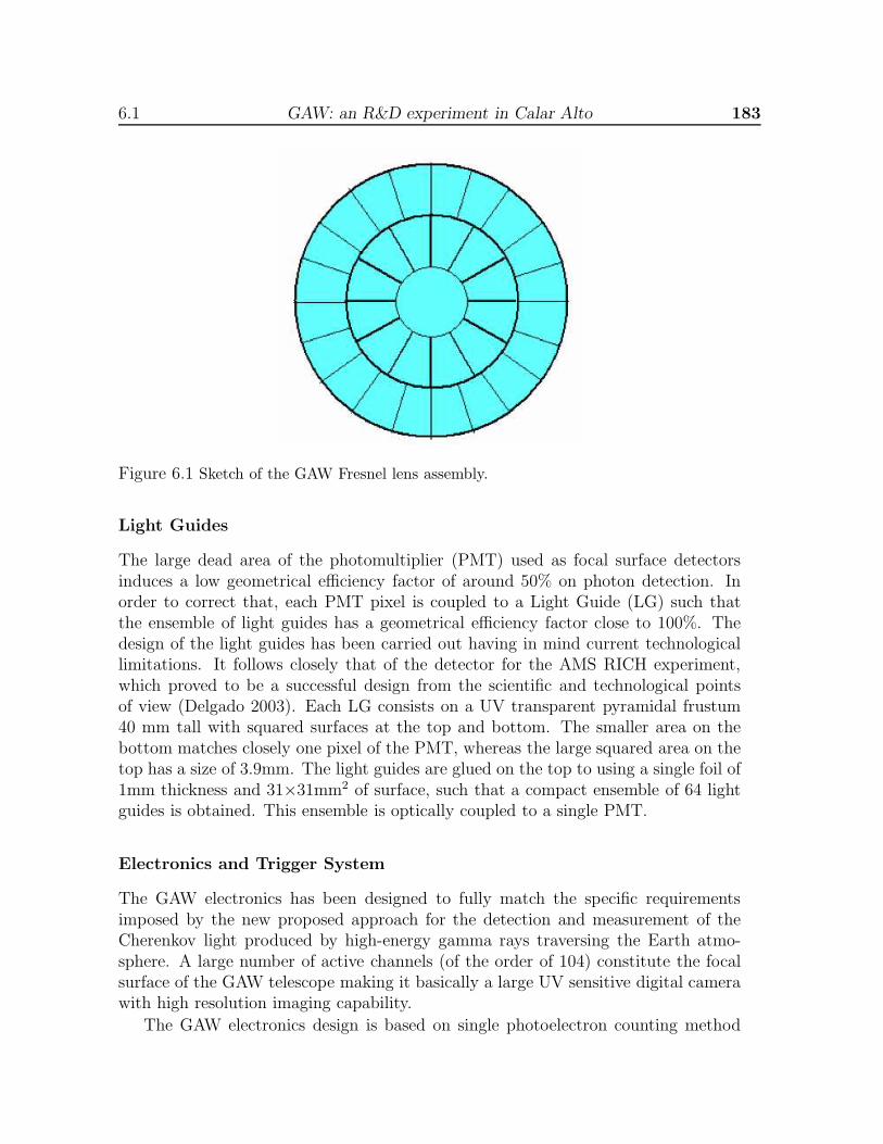
6.1 GAW: an R&D experiment in Calar Alto 183
Figure 6.1 Sketch of the GAW Fresnel lens assembly.
Light Guides
The large dead area of the photomultiplier (PMT) used as focal surface detectorsinduces a low geometrical efficiency factor of around 50% on photon detection. Inorder to correct that, each PMT pixel is coupled to a Light Guide (LG) such thatthe ensemble of light guides has a geometrical efficiency factor close to 100%. Thedesign of the light guides has been carried out having in mind current technologicallimitations. It follows closely that of the detector for the AMS RICH experiment,which proved to be a successful design from the scientific and technological pointsof view (Delgado 2003). Each LG consists on a UV transparent pyramidal frustum40 mm tall with squared surfaces at the top and bottom. The smaller area on thebottom matches closely one pixel of the PMT, whereas the large squared area on thetop has a size of 3.9mm. The light guides are glued on the top to using a single foil of1mm thickness and 31×31mm2 of surface, such that a compact ensemble of 64 lightguides is obtained. This ensemble is optically coupled to a single PMT.
Electronics and Trigger System
The GAW electronics has been designed to fully match the specific requirementsimposed by the new proposed approach for the detection and measurement of theCherenkov light produced by high-energy gamma rays traversing the Earth atmo-sphere. A large number of active channels (of the order of 104) constitute the focalsurface of the GAW telescope making it basically a large UV sensitive digital camerawith high resolution imaging capability.
The GAW electronics design is based on single photoelectron counting method
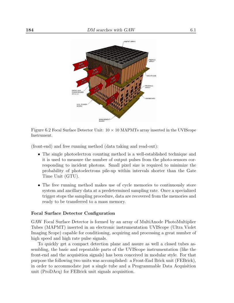
184 DM searches with GAW 6.1
Figure 6.2 Focal Surface Detector Unit: 10 × 10 MAPMTs array inserted in the UVIScopeInstrument.
(front-end) and free running method (data taking and read-out):
• The single photoelectron counting method is a well-established technique andit is used to measure the number of output pulses from the photo-sensors cor-responding to incident photons. Small pixel size is required to minimize theprobability of photoelectrons pile-up within intervals shorter than the GateTime Unit (GTU).
• The free running method makes use of cycle memories to continuously storesystem and ancillary data at a predetermined sampling rate. Once a specializedtrigger stops the sampling procedure, data are recovered from the memories andready to be transferred to a mass memory.
Focal Surface Detector Configuration
GAW Focal Surface Detector is formed by an array of MultiAnode PhotoMultiplierTubes (MAPMT) inserted in an electronic instrumentation UVIScope (Ultra VioletImaging Scope) capable for conditioning, acquiring and processing a great number ofhigh speed and high rate pulse signals.
To quickly get a compact detection plane and assure as well a closed tubes as-sembling, the basic and repeatable parts of the UVIScope instrumentation (like thefront-end and the acquisition signals) has been conceived in modular style. For thatpurpose the following two units was accomplished: a Front-End Brick unit (FEBrick),in order to accommodate just a single tube and a Programmable Data Acquisitionunit (ProDAcq) for FEBrick unit signals acquisition.

6.1 GAW: an R&D experiment in Calar Alto 185
Figure 6.3 Conceptual design of the GAW telescopes.
The whole apparatus gets the major requirements of the GAW Focal SurfaceDetector:
• Single Photon Sensitivity in the 300-600 nm band, which is the characteristicsCherenkov wavelengths band.
• Fast response (< 10 ns) to follow the very short Cherenkov light time duration.
• Low noise and good signal to noise ratio to detect faint signals.
• Imaging capability with moderate spatial resolution (order of mm).
• Large total Focal Surface area for large FoV application.
Telescopes
In Figure 6.3 we present the telescope tube drawings and dimensions. The threetelescopes will be identical with an alt-az mounting. The design and construction so-lutions of the telescopes do not offer major difficulties given the fact that the requiredtelescope performance is not very demanding in terms of pointing and tracking. Thismakes for example possible to use commercial encoders and telescope motor drives.The telescopes will be able to work with wind load up to 15 m/s. We plan to useCFK trusses for the focus system, which should be stable within ± 2 mm. The overalldetector weight will be about 500 kg. One detector unit (6 × 6) will be about 50kg. The overall dimension of the focal plane (fixed) is 2180 mm × 2180 mm × 1100mm. The idea is to interfacing the focal surface to the fixed focal plane by means ofan ad hoc home-made structure, starting from 6 × 6, the initial Focal Surface unit,and changing this structure in case we like to accommodate more units at the focalsurface or moving the first one detector unit.
On-Axis Expected Performance
The following figures present the telescope performance obtained from the analysisof the GAW array simulation data using the nominal performance of each telescope

186 DM searches with GAW 6.1
Figure 6.4 Collecting area of the GAW telescope array vs energy for on-axis Gamma Rayevents at two different pointing directions.
unit and of the whole array. Figure 6.4 gives the collecting area versus energy forgamma-ray events: values are derived from monoenergetic gamma ray event, in whichthe source is on axis with respect to the telescope, but at two different pointingdirections (θ=0 deg and θ=50 deg from zenith). Each point in the figure is computedmultiplying the fiducial area (1520 × 1520 m2) by the ratio between triggered eventsand generated events.
Taking into account the GAW performance for gamma events and having also an-alyzed the hadronic events file, we also computed: the signal-to-noise ratio reachablein one hour observation for a Crab-like source, the time in which we can reach 5 stan-dard deviations, and the minimum detectable flux. In the sensitivity computation weconsider only the hadron contribution because the contribution of the electron com-ponent at GAW energy is completely negligible. The results are reported in Table6.1 while in upper panel of Figure 6.5 the flux limit in 50 h observation in functionof the lower energy threshold is shown.
GAW Large Field of View Capability
Highlight of the GAW experiment is its large field of view that is foreseen to reachin Phase II, at the completion of the focal surface, 24 × 24. Typical focal detectordiameter values for the present and planned IACTs range from 3 deg to 5 deg; byconsidering that the most external ring (∼1) is not useful due to the intrinsic sizeof the Cherenkov image, the actual ratio between GAW and the other IACTs is afactor of 35. This can be used to address GAW to perform high sensitivity survey of
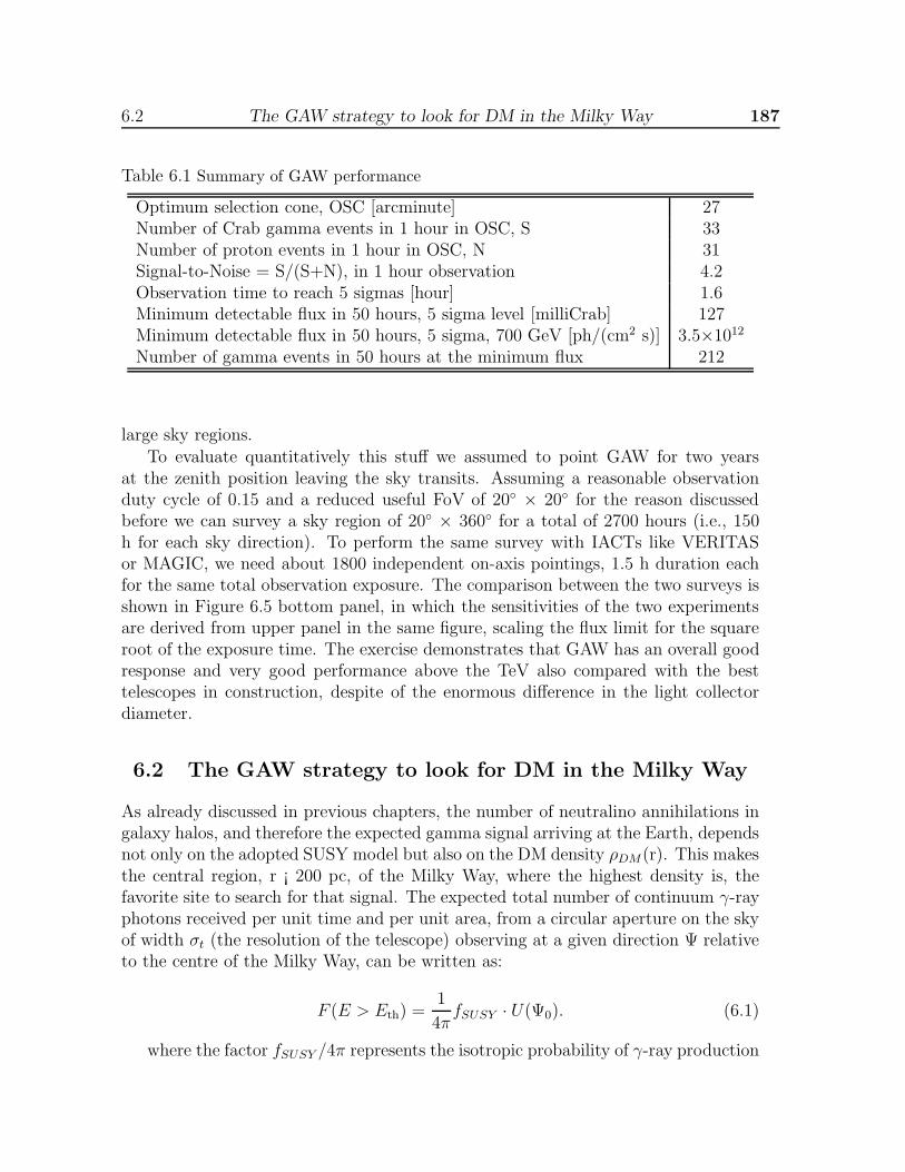
6.2 The GAW strategy to look for DM in the Milky Way 187
Table 6.1 Summary of GAW performance
Optimum selection cone, OSC [arcminute] 27Number of Crab gamma events in 1 hour in OSC, S 33Number of proton events in 1 hour in OSC, N 31Signal-to-Noise = S/(S+N), in 1 hour observation 4.2Observation time to reach 5 sigmas [hour] 1.6Minimum detectable flux in 50 hours, 5 sigma level [milliCrab] 127Minimum detectable flux in 50 hours, 5 sigma, 700 GeV [ph/(cm2 s)] 3.5×10¹²
Number of gamma events in 50 hours at the minimum flux 212
large sky regions.To evaluate quantitatively this stuff we assumed to point GAW for two years
at the zenith position leaving the sky transits. Assuming a reasonable observationduty cycle of 0.15 and a reduced useful FoV of 20 × 20 for the reason discussedbefore we can survey a sky region of 20 × 360 for a total of 2700 hours (i.e., 150h for each sky direction). To perform the same survey with IACTs like VERITASor MAGIC, we need about 1800 independent on-axis pointings, 1.5 h duration eachfor the same total observation exposure. The comparison between the two surveys isshown in Figure 6.5 bottom panel, in which the sensitivities of the two experimentsare derived from upper panel in the same figure, scaling the flux limit for the squareroot of the exposure time. The exercise demonstrates that GAW has an overall goodresponse and very good performance above the TeV also compared with the besttelescopes in construction, despite of the enormous difference in the light collectordiameter.
6.2 The GAW strategy to look for DM in the Milky Way
As already discussed in previous chapters, the number of neutralino annihilations ingalaxy halos, and therefore the expected gamma signal arriving at the Earth, dependsnot only on the adopted SUSY model but also on the DM density ρDM(r). This makesthe central region, r ¡ 200 pc, of the Milky Way, where the highest density is, thefavorite site to search for that signal. The expected total number of continuum γ-rayphotons received per unit time and per unit area, from a circular aperture on the skyof width σt (the resolution of the telescope) observing at a given direction Ψ relativeto the centre of the Milky Way, can be written as:
F (E > Eth) =1
4πfSUSY · U(Ψ0). (6.1)
where the factor fSUSY /4π represents the isotropic probability of γ-ray production

188 DM searches with GAW 6.2
Figure 6.5 Upper panel: GAW sensitivity for known point source. For comparison, theflux of the Crab Nebula and the sensitivity of other TeV experiments are also shown..Bottom panel: GAW sensitivity limit for a two years survey of a large sky region, 7200square degrees, compared with a hypothetical survey made by a VERITAS-like Cherenkovtelescope in an equivalent overall observation exposure time.
per unit of DM density and depends only on the physics of annihilating neutralinoparticles. It can be determined for any SUSY scenario given the neutralino properties.The fSUSY parameter decreases with the energy threshold Eth and can change by alarge factor (up to four orders of magnitude in the minimal supergravity, mSUGRA,
6.2 The GAW strategy to look for DM in the Milky Way 189
scenario). All the astrophysical properties (such as the DM distribution and geometryconsiderations) appear only in the factor U(Ψ). This factor also accounts for thetelescope beam smearing, and it is the integral of the line-of-sight of the square of theDM density along the direction Ψ. A cuspy DM halo, ρ ∝ r−α, predicted by ΛCDMsimulations is often assumed for the calculations of U(Ψ). The value of α varies from1 (NFW density profile, Navarro, Frenk & White 1997) to 1.5 (Moore DM profile,Moore et al. 1998), although observational data seems to prefer cored profiles withα <1.
Recent developments in the modelization of the DM distribution in our Galaxypointed out the necessity to consider some physical processes previously neglectedsuch as the effect of the baryonic compression in the halo, which increases significantlythe DM density in the central region of the Milky Way. On the other hand, thenon-universality in the scalar and gaugino sectors of supergravity models can alsoincrease significantly the neutralino annihilation cross-section. The combination ofboth effects results in much higher γ-ray flux prediction from the Galactic Center,that would be detectable by present and future experiments like HESS, MAGIC,VERITAS, CANGAROO, Fermi and our proposed experiment GAW at Calar Alto(Prada et al. 2004; Mambrini et al. 2005 and references therein). In Figure 6.6 weshow the expected gamma-ray continuum flux as a function of the angular distancefrom the Galactic Center, for the compressed DM density profiles provided by ourMilky Way models in Prada et al. (2004). The flux is given in units of fSUSY /10−32.The flux profiles were determined for a typical IACT of resolution σt=0.1.
A TeV gamma-ray signal in the direction of the Galactic Centre (GC) has al-ready been detected by the HESS experiment in Namibia (Aharonian et al. 2004).The 12σ-detection at TeV energies is consistent with the source being point-like, ac-tually HESS J1745-290 (Aharonian et al. 2005), without further indication for anextended emission. It must be noted that the presence of an extended component inthe gamma radiation coming from the central regions of the Milky Way is expectedfrom the SUSY DM annihilation signal as shown in Figure 6.6. The flux and spec-trum of this source measured by HESS differ substantially from previous results, inparticular those reported by CANGAROO and EGRET (see Mambrini et al. 2005for a detail comparison). The gamma-ray source reported by HESS exhibits a muchharder power-law energy spectrum with spectral index of about -2.2 and extends upto 9 TeV. The interpretation of this signal as being due to the annihilation products ofSUSY DM yield a neutralino of mass > 12 TeV. Actually such a heavy LSP neutralinois not natural in the framework of consistent supergravity model when we impose therenormalization group equations and radiative electroweak symmetry breaking (Aha-ronian et al. 2004; Mambrini et al. 2005). Furthermore, an extended emission wasalso discovered in the GC area, but it correlates very well with already known densemolecular clouds (Aharonian et al. 2006). Recently, new HESS data on the GChave been published and a reanalysis has been carried out by the HESS collaboration(Aharonian et al. 2006b). In this work, they especially explore the possibility that
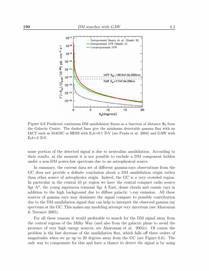
190 DM searches with GAW 6.2
Figure 6.6 Predicted continuum DM annihilation fluxes as a function of distance Φ0 fromthe Galactic Centre. The dashed lines give the minimum detectable gamma flux with anIACT such as MAGIC or HESS with Eth=0.1 TeV (see Prada et al. 2004) and GAW withEth=3 TeV.
some portion of the detected signal is due to neutralino annihilation. According totheir results, at the moment it is not possible to exclude a DM component hiddenunder a non-DM power-law spectrum due to an astrophysical source.
In summary, the current data set of different gamma-rays observations from theGC does not provide a definite conclusion about a DM annihilation origin ratherthan other source of astrophysics origin. Indeed, the GC is a very crowded region.In particular in the central 10 pc region we have the central compact radio sourceSgr A*, the young supernova remnant Sgr A East, dense clouds and cosmic rays inaddition to the high background due to diffuse galactic γ-ray emission. All thesesources of gamma rays may dominate the signal compare to possible contributiondue to the DM annihilation signal that can help to interpret the observed gamma rayspectrum at the GC. This makes any modeling attempt very uncertain (see Aharonian& Neronov 2005).
For all these reasons it would preferable to search for the DM signal away fromthe central regions of the Milky Way (and also from the galactic plane to avoid thepresence of very high energy sources, see Aharonian et al. 2005e). Of course theproblem is the fast decrease of the annihilation flux, which falls off three orders ofmagnitudes when we go up to 20 degrees away from the GC (see Figure 6.6). Theonly way to compensate for this and have a chance to detect the signal is by using
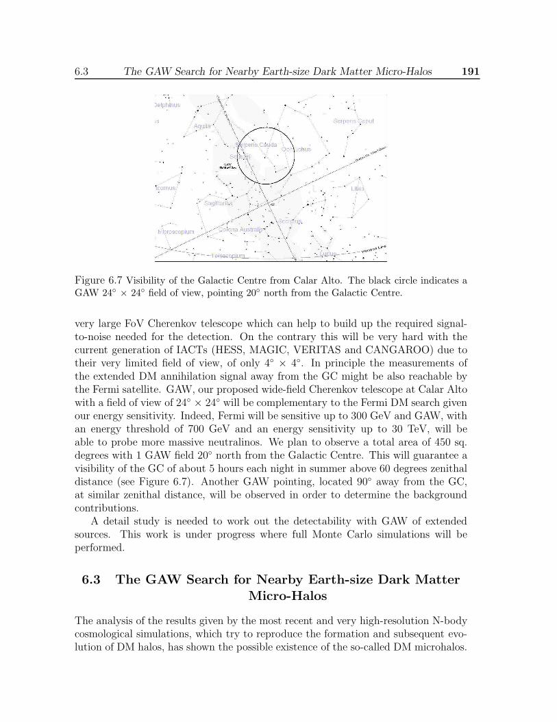
6.3 The GAW Search for Nearby Earth-size Dark Matter Micro-Halos 191
Figure 6.7 Visibility of the Galactic Centre from Calar Alto. The black circle indicates aGAW 24 × 24 field of view, pointing 20 north from the Galactic Centre.
very large FoV Cherenkov telescope which can help to build up the required signal-to-noise needed for the detection. On the contrary this will be very hard with thecurrent generation of IACTs (HESS, MAGIC, VERITAS and CANGAROO) due totheir very limited field of view, of only 4 × 4. In principle the measurements ofthe extended DM annihilation signal away from the GC might be also reachable bythe Fermi satellite. GAW, our proposed wide-field Cherenkov telescope at Calar Altowith a field of view of 24 × 24 will be complementary to the Fermi DM search givenour energy sensitivity. Indeed, Fermi will be sensitive up to 300 GeV and GAW, withan energy threshold of 700 GeV and an energy sensitivity up to 30 TeV, will beable to probe more massive neutralinos. We plan to observe a total area of 450 sq.degrees with 1 GAW field 20 north from the Galactic Centre. This will guarantee avisibility of the GC of about 5 hours each night in summer above 60 degrees zenithaldistance (see Figure 6.7). Another GAW pointing, located 90 away from the GC,at similar zenithal distance, will be observed in order to determine the backgroundcontributions.
A detail study is needed to work out the detectability with GAW of extendedsources. This work is under progress where full Monte Carlo simulations will beperformed.
6.3 The GAW Search for Nearby Earth-size Dark MatterMicro-Halos
The analysis of the results given by the most recent and very high-resolution N-bodycosmological simulations, which try to reproduce the formation and subsequent evo-lution of DM halos, has shown the possible existence of the so-called DM microhalos.
192 DM searches with GAW 6.3
These microhalos would be the first collapsed structures formed in the Universe andthey would have survived until now thanks to its high concentration of matter (seee.g. Moore et al. 2005, Zhao et al. 2005, Pieri et al. 2005, Diemand et al. 2005).These microhalos, with masses similar to the Earth and typical size of the Solar Sys-tem, would be within a more massive DM halo. In fact, the Milky Way should containthousands of them, since for example densities of the order of 100 microhalos/parsec3are considered for the solar galactocentric radius (Pieri et al. 2005). Because of that,microhalos are a suitable target for a search of DM annihilation γ-ray signal usingCherenkov telescopes. Despite of its small size and low content in DM compared togalactic size halos, its extreme proximity (perhaps the nearest one will be less than0.1 parsec) makes possible to raise its detectability.
GAW constitutes the ideal instrument to search for these DM microhalos, thanksto its large field of view of 24 × 24. Moreover, we plan to survey a large area of thesky in the second phase of the experiment, more specifically 20 × 360 in two years.Studying large areas of the sky is essential if we want to detect these microhalos,because we do not know a priori their exact positions, even when they are expectedto be isotropically distributed in the Milky Way (except in the very centre, wherethey can not survive because of the high tidal forces). Furthermore, the GAW surveywill be performed keeping the telescope pointing to the zenith at all time (withoutany kind of sky tracking) so that we can obtain data from different regions of thegalaxy.
It becomes possible to make some rough calculations in order to obtain the prob-ability for GAW to be able to detect the γ-ray signal coming from effective DMannihilation inside nearby microhalos. Given the high uncertainties concerning boththe DM particle properties and the physical parameters of the microhalo, we can onlydo some simple assumptions:
1. The microhalos have a constant density core within its scale radius, ρs = 1.29× 10⁻²² g cm−3 (Diemand et al. 2005).
2. We will assume the scale radius rs for the microhalos to be around 0.0025 parsec(Diemand et al. 2005).
3. Density of microhalos in the solar neighborhood equal to 500 microhalos/parsec−3
(Diemand et al. 2005).
4. Neutralino fSUSY = 10−32 ph GeV2 cm3 s−1 (Prada et al. 2004, Sanchez-Condeet al. 2007).
5. GAW flux sensitivity above 1 TeV equal to FGAW = 3×10¹² ph cm−2 s−1 (esti-mated sensitivity for a two years 20 × 360 survey).
Within this scenario we can estimate the number of microhalos that it would bepossible to detect in our 7200 square degrees survey. The luminosity of one microhalo,
6.4 GAW Prospects for Dark Matter detection from IMBHs 193
using the above assumptions, is equal to LMH = fSUSY ρs rs / 3 = 8 × 1024 ph s−1.If we use the minimum flux that we can detect with GAW above 1 TeV, we obtainaround 0.15 parsec for the maximum distance at which a microhalo could be detectedwith GAW. With a value of 500 pc3 for the density of microhalos, we may detect 1.2microhalos in our 7200 square degrees survey. According to these calculations thedetection of one of these microhalos by GAW may be difficult but still possible,although a more detailed study is necessary.
6.4 GAW Prospects for Dark Matter detection from
Intermediate-Mass Black Holes
The detection of γ-rays from DM enhancements around black holes with masses inthe interval from 100 to 106 solar masses has been studied by Bertone et al. (2005).For typical neutralino properties they have shown that these back holes can be brightγ-rays sources, and detectable with a wide field IACT such as Fermi or GAW. Theprospects of detection with Fermi are very promising in the energy domain up to300 GeV. GAW at higher energies will have also a serious chance to detect theseintermediate mass black holes, as shown in Figure 6.8 where the number of blackholes producing some γ-ray flux as a function of the GAW flux limit for a pointsource above 400 GeV (blue vertical line) and 2 TeV (black vertical line) is plotted.The yellow shaded region is for a neutralino with a mass of 1 TeV and < σ v > = 3×10⁻²⁶ cm3 s−1. The red shaded region is for 5 TeV neutralino mass, with < σ v >= 3 ×10⁻²⁶ cm3 s−1.
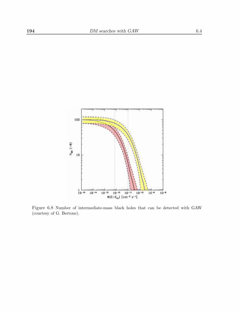
194 DM searches with GAW 6.4
Figure 6.8 Number of intermediate-mass black holes that can be detected with GAW(courtesy of G. Bertone).

Bibliography
Aharonian F.A. et al. , 2004, A&A, 425, L13
Aharonian F.A. et al. , 2005, Science, 309, 746
Aharonian F. et al. , 2006, Nature, 439, 695
Aharonian F. et al. , 2006b, Phys. Rev. Letters, 97, 221102
Aharonian F.A. and Neronov A., 2005, ApJ, 619, 306
Arqueros F. et al. , 1999, Proc. 26th ICRC, 5, 215
Bernlohr K., 2000, Astropart. Phys., 12, 255
Bertone G., Zentner A. R. and Silk J., 2005, Physical Review D, 72, 103517
Chantell M.C. et al. , 1998, Nucl. Instrum. Meth., Phys.Res. A, 408, 468
Cusumano G. et al. [GAW Collaboration], Proc. of the 30th ICRC, Merida, Mexico,3-11 July 2007, 3, 1313
Delgado C., 2003, PhD Thesis, Universitat Autonoma de Madrid
Diemand J., Moore B., Stadel J., 2005, Nature, 433, 389
Giebels B. et al. , 1998, Nucl. Instrum. Meth. A, 412, 329
Hartman R.C. et al. , 1999, ApJ Suppl Series, 123, 79
Kabuki S., et al. , 2003, Nucl. Instrum. Meth. A, 500, 318
Krennrich F., et al. , 2001, ApJ, 560, L45
Lorenz et al. , 1999, AIP Conference Proceedings, 515, 510
Mambrini Y., Munoz C., Nezri E. and Prada F., 2006, JCAP, 01, 010
196 BIBLIOGRAPHY 6.4
Moore B., Diemand J., Stadel J., Quinn T., 2005, astro-ph/0502213
Navarro J. F., Frenk C. S. and White S. D. M., 1997, ApJ, 490, 493
Moore B., Governato F., Quinn T., Stadel J. and Lake G., 1998, MNRAS, 499, L5
Pieri L., Branchini E., and Hofmann S., 2005, Phys. Rev. Letters, 95, 211301
Prada F., Klypin A., Flix J., Martınez M. and Simonneau E., 2004, Phys. Rev.Letters, 93, 241301
Sanchez-Conde M A, Prada F, Lokas E L, Gomez M E, Wojtak R and Moles M,2007,Phys. Rev. D. 76 123509
Weekes T.C., et al. , 2002, Astropart. Phys., 17, 221
Weekes T.C., 2003, Plenary Talk at 28th ICRC
Zhao H., Taylor J.E., Silk J., Hooper D. 2005, astro-ph/0502049
Zweerink, J., et al. 1999, Proc. 26th ICRC, 5, 223

Part III
DM searches with the MAGIC-Itelescope

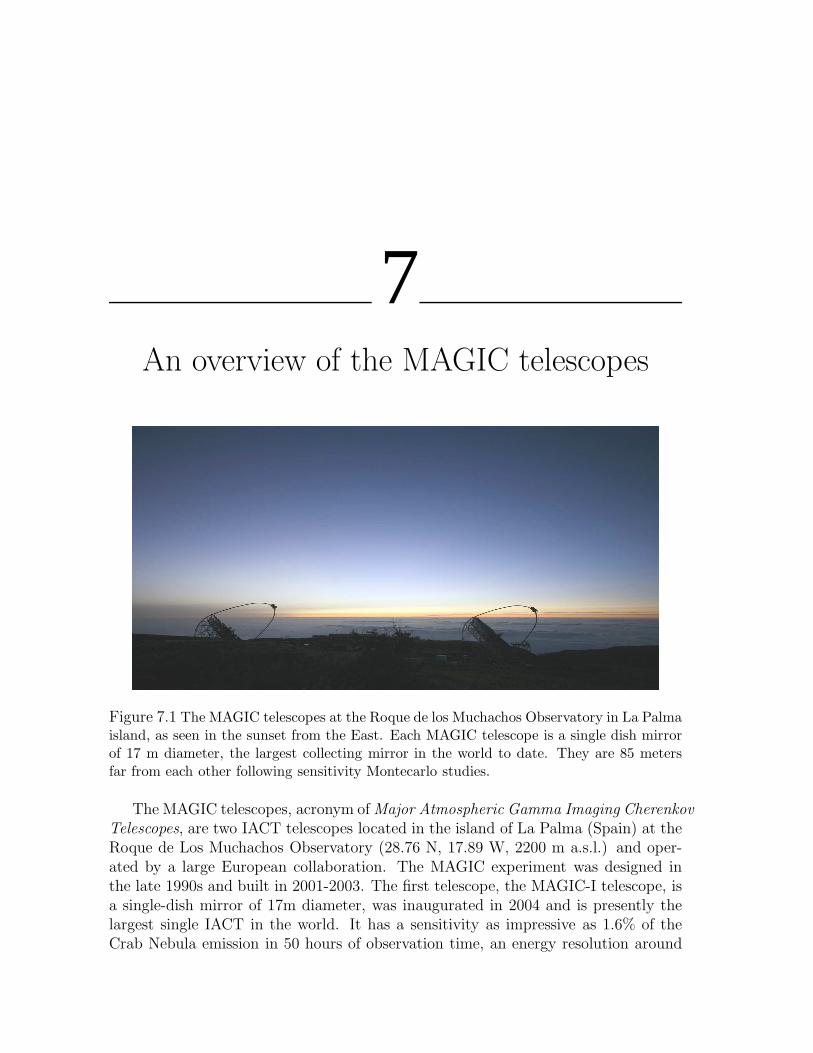
7An overview of the MAGIC telescopes
Figure 7.1 The MAGIC telescopes at the Roque de los Muchachos Observatory in La Palmaisland, as seen in the sunset from the East. Each MAGIC telescope is a single dish mirrorof 17 m diameter, the largest collecting mirror in the world to date. They are 85 metersfar from each other following sensitivity Montecarlo studies.
The MAGIC telescopes, acronym of Major Atmospheric Gamma Imaging CherenkovTelescopes, are two IACT telescopes located in the island of La Palma (Spain) at theRoque de Los Muchachos Observatory (28.76 N, 17.89 W, 2200 m a.s.l.) and oper-ated by a large European collaboration. The MAGIC experiment was designed inthe late 1990s and built in 2001-2003. The first telescope, the MAGIC-I telescope, isa single-dish mirror of 17m diameter, was inaugurated in 2004 and is presently thelargest single IACT in the world. It has a sensitivity as impressive as 1.6% of theCrab Nebula emission in 50 hours of observation time, an energy resolution around
200 An overview of the MAGIC telescopes 7.1
25% at 100 GeV and an angular resolution slightly better than 0.1 deg at this sameenergy. A second MAGIC telescope -located 85 meters away from MAGIC-I and withsame dimensions than the telescope currently in operation- was inaugurated last April2009 and is planned to start data taking this same year 2009. MAGIC-II will surelymake possible to improve the excellent marks reached up to now thanks to a factor2 better sensitivity, a better energy resolution and an even lower energy threshold.The project is funded primarily by the funding agencies BMFB (Germany), MPG(Germany), INFN (Italy), MICINN (Spain), and the ETH Zurich (Switzerland).
Some key points and goals of the MAGIC telescopes are:
• High Cherenkov photon-to-photoelectron conversion efficiency.
• The largest collecting mirror (17 m diameter) in the world to date.
• Lowest energy threshold ever obtained with an IACT. This fact, together witha high sensitivity, makes possible to explore the energy gap between ∼25 GeVand 150 GeV.
• Fast movement of the telescopes to anywhere in the sky (in less than ∼40seconds), with the clear intention of observing prompt emission from gamma-ray bursts (GRB) following satellite alerts.
• Capability to operate the telescopes even with moonlight (Albert et al. 2007).This makes possible to increase the observation time by roughly a factor 2.
• Steoroscopic system, once the commissioning phase for MAGIC-II is over andthis telescope is fully operative. This observation mode is expected to lowereven more the energy threshold of the experiment, as well as to increase thesensitivity by a factor 2.
In the following we will briefly review the main characteristics of the MAGICexperiment. This review is only strictly valid for the MAGIC-I telescope. MAGIC-II(recently inaugurated) is essentially a clone of MAGIC-I with some technical improve-ments, and will be presented separately in section 7.3. A more detailed description ofthe whole experiment can be found in Baixeras et al. (2003) and Borla et al. (2009).
7.1 MAGIC: the lowest energy threshold of current IACTs
The MAGIC telescope has been built with the clear goal to lower the energy thresh-old for gamma rays. For many unanswered physics questions, a low energy thresholdholds the key. The general argument is the absolute necessity to explore the elec-tromagnetic spectrum at all wavelengths, and the absence, at the present time, ofany instrument exploring the energy region between some tens of GeV and several

7.2 MAGIC: the lowest energy threshold of current IACTs 201
hundred GeV with adequate sensitivity. At lower energies, satellite experiments, inparticular EGRET, have contributed substantial knowledge. Their energy range andsensitivity is being very much improved by the EGRET successor, Fermi, (successfullylaunched in June, 2008), but even Fermi has the limit of detector size, and will have tobe supplemented by complementary terrestrial observations. Pre-MAGIC gamma-raytelescopes, on the other hand, have typically an energy threshold of several hundredGeV.
The interest to this relatively narrow energy band, from 10 to 100 GeV, is mo-tivated not only by the natural desire to enter a new domain which remains a terraincognita, but also because it provides a bridge between the high and very high as-tronomies, and thus may allow key inspections of the current concepts concerningboth the GeV and TeV regimes. Moreover, there are good scientific reasons to lowerthe energy threshold, such as the careful study of the gamma-ray horizon, Cold DarkMatter, quantum gravity, Gamma Ray Bursts, supernova remnants and plerions, pul-sars, AGNs, the diffuse photon background, etc. In each of the mentioned fields, alow energy threshold would mean the access to a invaluable and critical informationon several physical processes.
Figure 7.2 The MAGIC-I telescope in the sunset. The camera box is clearly seen 17 metersin front of the 239 m2 reflecting surface, which consists of 956 square mirrors of 50 cm side.The whole structure wights around 60 tons.

202 An overview of the MAGIC telescopes 7.2
7.2 Main technical characteristics
The most critical technical parameters of MAGIC could be summarized as follows(see Fig. 7.2):
• Active mirror surface 239 sq.m., made of square elements 49.5cm x 49.5cm;f/D = 1.03.
• Support frame of carbon fibre made for minimum weight and maximum stiff-ness.
• Hexagonal camera of 1.05 m diameter, with an inner area of 396 PMTs of 1”diameter each, surrounded by 180 PMTs of 1.5” diameter, arranged in fourconcentric rings. All tubes have an effective quantum efficiency of 25 to 30%.
• The camera is kept as light as possible, held by an aluminum support stiffenedby a web of thin cables.
• Analogue signals are transmitted from the camera to the control house viaoptical fibers; only the amplifiers and laser diode modulators for transmissionare inside the camera housing. Digitization is achieved by new FADCs with asampling frequency of 2 GHz.
• The threshold for gamma detection is at present as low as ∼50 GeV for lowzenith angles. In addition, by means of a recently developed technical config-uration, it was possible to reach an energy threshold around 25 GeV for somespecific observations (Aliu et al. 2008).
• The average time to reposition the MAGIC telescopes anywhere on the observ-able sky is less than 40 seconds (despite a moving weight of ∼60 tons).
FrameThe frame of each telescope roughly follows the concept of a large (17 m diameter)solar concentrator with alt/az mount, which was already built and tested a few yearsago as part of the German solar power research program. The main mirror supportdish consists of a three layer space frame made from carbon fiber-epoxy tubes, whichare lighter and more rigid than aluminum. Knots to join the tubes are made fromaluminum.The weight of the frame, including the lower drive ring for azimuthal movement, isabout 9 tons (the whole telescope and the undercarriage weights 64 tons). This framestructure keeps the inertia of the telescope low enough for it to be repositioned within40 s at any position in the sky; this allows, for the first time, the capability of fastrepositioning to follow-up GRBs, which is a extremely valuable and unique featureamong current IACTs. The frame structure guarantees wind resistance up to < 170
7.2 Main technical characteristics 203
km/h and stability for complete ice coverage up to 3 cm thickness.
DriveThe MAGIC telescope is driven by high precision servo-motors. The azimuth axisof the tele- scope is equipped with two 11 kW motors, while the elevation axis has asingle 11 kW motor. In azimuth the movement is limited to a range of 450, while inzenith to -10.
The position of the telescope is measured in the mechanical telescope frame by threeabsolute 14-bit shaft-encoders. With this configuration is possible to monitor the tele-scope position with an accuracy of 0.02. By using a high sensitivity CCD cameramounted on the reflector frame, the precision of the tracking system can be verifiedby monitoring both LEDs installed in the camera frame and stars from the celestialbackground (Starguider System). With this star-field tracking monitor system it hasbeen measured that the telescope tracks to better than a 1/10 of a pixel size.
MirrorsThe Cherenkov light produced by air showers is collected and focused to the cameraby an octagonal shape tessellated mirror reflector of 239 m2 area. The overall cur-vature of the reflector is parabolic to minimize the spread in the arrival time of theCherenkov photons to the camera plane. To assure high optical quality images atthe camera, the focal length to diameter ratio (f/D) is set to 1 (to lower astigmatismover 3.6 deg diameter in the focal plane). The 239 m2 reflecting surface consistsof 956 square mirrors of 50 cm side and 34 to 36 m radius of spherical curvature,depending on the position of the mirror in the parabolic dish. Each one is made ofan aluminium honeycomb structure; a heating/drying system in case of ice or dewformation; a reflecting 5 mm-thick plate of diamond-milled aluminum and a quartzcoating layer. Mirrors are grouped into panels of four; each panel is provided withtwo motors and a laser pointing to the camera lids, allowing a fine focusing duringdatataking through the Active Mirror Control. This is necessary in order to correctthe residual deformation of the reflector when the telescope is repositioned. The sur-face global reflectivity is about 85% in the wavelength range 300-650 nm.
CameraThe camera is the most critical element in the performance of a Cherenkov telescope.In the camera, the conversion from Cherenkov photons to photo-electrons takes placeand this affects the energy threshold, as it depends directly on this conversion ef-ficiency. In addition, the quality of the shower images which are recorded in thecamera is relevant for the posterior gamma/hadron separation. The MAGIC-I cam-era is composed by an hexagonal board of 1.5 m diameter, placed in the mirror focalplane, which hosts 577 high Quantum Efficiency photomultipliers, of which 397 1”inner pixels and 180 1.5” outer pixels. Light from the reflector is transmitted to eachPMT through a Winston cone with an hexagonal end, so that there are no blind

204 An overview of the MAGIC telescopes 7.2
regions in the camera; the total Field Of View (FoV) results equal to 3.5×3.8. Aspecial wavelength-shifter coating enhances QE up to an average 20% between 250and 700 nm wavelength. Since typical duration of Cherenkov flashes is on the order ofa few nanoseconds, PMTs are designed to give a fast response with 1 ns FWHM. HighVoltage supply is independent for each PMT and remotely controlled by the CameraControl software. Finally, the camera is equipped with heating and cooling systemsto prevent the reaching of the dew point and to dissipate the heat from phototubes.
Figure 7.3 Left: The MAGIC camera with the lids opened. The hexagonal shape, composedby 577 PMTs, is clearly seen in the picture. Right: Pixel scheme of the camera, with 3971” inner pixels (blue) and 180 1.5” outer pixels (red). The total FoV is 3.5×3.8.
In summary, the MAGIC camera has the following features:
• Fine granularity: it allows to better deals with low energy shower images andalso allows for a more efficient gamma/hadron discrimination. Moreover, theintegrated noise per pixel is reduced and trigger threshold at the discriminatorlevel can be lowered. This facilitates the reduction of the energy threshold.
• Large Field of View: the 3.5×3.8 camera FoV makes possible to recordmost of shower images (showers up to 10 TeV for low zenith angles).
• Low noise: the detection of Cherenkov pulses suffers from a strong backgroundof Night Sky Background photons. Therefore, the response of the whole systemhas to be fast in order to reduce the width of the pulses at trigger level to onlya few nanoseconds.
• Low Gain operation: it reduces the noise level recorded by the camera. Inorder to be able to operate the telescope under moonlight, we are forced tooperate with a relatively low gain around ∼104, in contrast to typical gainsaround 106.
Readout and TriggerAnalogue signals from PMTs are preamplified and then transmitted via optical fibers

7.3 The MAGIC-II stereoscopic system 205
to the electronics room located in the Control House, where they will be processed.Only the amplifiers and laser diode modulators for transmission are inside the camerahousing. Digitization is achieved by new FADCs with a sampling frequency of 2 GHz.
As for the trigger system, it has the purpose of a first discrimination between signaland background. At this very early stage, however, it is not possible to perform arejection of hadron-like images with respect to the gamma-like ones: this should bedone later in an offline analysis chain. The trigger is segmented in three levels:
Level 0: it acts as a flag for lighted PMTs. A phototube is considered lighted if itscurrent exceeds a fixed threshold; if this happens, a digital signal is generatedby L0 and processed by the next trigger stages.
Level 1: this level involves only 325 inner pixels, grouped into 19 overlappingmacrocells of 37 pixels each. A temporal coincidence (few ns) among a certainnumber of neighboring pixels within a macrocell is required: this constraint ismotivated with the intention of selecting compact configurations like the ellipticshapes typical from Cherenkov flashes.
Level 2: the last trigger stage performs a fast evaluation of size, shape and orien-tation of the image, in order to make an effective background rejection and toreduce the trigger rate.
The digitized data which successfully approves all the trigger levels are stored in disksand backed-up into tapes. In addition, every day, data from the last night are copiedto the Barcelona and Wurzburg Datacenters, where they are kept and made availableto the analyzers.
7.3 The MAGIC-II stereoscopic system
As already commented, a second MAGIC telescope was inaugurated last April 2009at La Palma. Therefore, now MAGIC is a stereoscopic system of IACTs with the twolargest dishes in the world. The second 17m diameter telescope is currently undercommissioning and is located 85 meters far from MAGIC-I. The MAGIC experiment,with its large reflector area, high quantum efficiency photomultipliers, optical signaltransmission and fast digitization, will benefit from an improved shower reconstruc-tion and increased background rejection thanks to the simultaneous observation byusing two telescopes. The stereo observation will result in a better angular resolution,with an improvement of 20%, better energy estimation, with an energy resolutionimproving from 25% to 15% and higher cosmic-ray background rejection. The fluxsensitivity of the 2-telescope system is about 3 times better than that of a singletelescope (MAGIC-I) at energies below 200 GeV (see Fig. 7.4).
The structure of the second telescope is almost identical with that of the MAGIC-I telescope. The lightweight reinforced carbon-fiber reflector frame, the drive system
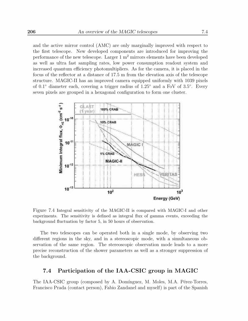
206 An overview of the MAGIC telescopes 7.4
and the active mirror control (AMC) are only marginally improved with respect tothe first telescope. New developed components are introduced for improving theperformance of the new telescope. Larger 1 m2 mirrors elements have been developedas well as ultra fast sampling rates, low power consumption readout system andincreased quantum efficiency photomultipliers. As for the camera, it is placed in thefocus of the reflector at a distance of 17.5 m from the elevation axis of the telescopestructure. MAGIC-II has an improved camera equipped uniformly with 1039 pixelsof 0.1 diameter each, covering a trigger radius of 1.25 and a FoV of 3.5. Everyseven pixels are grouped in a hexagonal configuration to form one cluster.
Figure 7.4 Integral sensitivity of the MAGIC-II is compared with MAGIC-I and otherexperiments. The sensitivity is defined as integral flux of gamma events, exceeding thebackground fluctuation by factor 5, in 50 hours of observation.
The two telescopes can be operated both in a single mode, by observing twodifferent regions in the sky, and in a stereoscopic mode, with a simultaneous ob-servation of the same region. The stereoscopic observation mode leads to a moreprecise reconstruction of the shower parameters as well as a stronger suppression ofthe background.
7.4 Participation of the IAA-CSIC group in MAGIC
The IAA-CSIC group (composed by A. Domınguez, M. Moles, M.A. Perez-Torres,Francisco Prada (contact person), Fabio Zandanel and myself) is part of the Spanish
7.4 Participation of the IAA-CSIC group in MAGIC 207
participation in MAGIC since November 2006. At present, our group invests a largeeffort in different scientific and technical aspects inside the MAGIC Collaboration.In particular, and given our experience and research interests, we are deeply involvedin the Dark Matter and Exotic Physics Working Group from the very beginning ofour membership to the Collaboration. More recently, we crucially contributed to thecreation of the Clusters Working Group as part of a new and ambitious observationalstrategy to look for gamma-ray emissions in galaxy clusters. Finally, we also impor-tantly contribute to the scientific activities carried out inside the Galactic and AGNsWorking Groups. In the following, I will summarize my main research activities insidethe MAGIC Collaboration:
1. Dark Matter Working Group (DMWG): The IAA-CSIC group has been involvedin two internal proposals for the observation of two dwarf satellites of the MilkyWay in the context of DM searches: Draco and Willman 1. In the case ofDraco, a previous work led by myself (Sanchez-Conde et al. 2007) was thebasis for the DMWG to select the most likely DM density profile parameters,needed for a posterior comparison with the MAGIC data. As for Willman 1,I was co-P.I. of the observational proposal and strongly contributed into theastrophysical background. Both objects were finally observed by MAGIC, andboth observational campaigns led to two publications (Albert et al. 2008; Aliuet al. 2009). Both works are described in Chapters 8 and 9.
2. Galaxy Clusters Working Group (GCWG). The IAA-CSIC group made a greateffort to start a galaxy cluster observation campaign with the MAGIC tele-scope. This proposal led, as a first result, to the recent observation of a promis-ing galaxy cluster. Although the data analysis shows no gamma signal, thisobservation represented the first galaxy cluster observation by MAGIC. Fur-thermore, we will start a similar campaign also during this year 2009, probablyfor the same object in order to be able to put stringent constraints on funda-mental scientific questions concerning the mechanisms of gamma emissions inclusters. I was specially involved in the scientific justification to perform suchkind of observations in the context of DM searches in galaxy clusters, makingpredictions of the expected DM annihilation flux at Earth in a scenario wherethe neutralino is the DM particle. At present, I am also responsible of the writeup of the DM section in the paper to be submitted early.
The participation of the IAA-CSIC group in MAGIC includes important technicaltasks as well. In particular, and together with other MAGIC institutions, we havebeen involved and are responsible of the data daily checks. Daily checks are neededin order to ensure an appropriate quality data to the rest of the Collaboration, aswell as to quickly resolve or inform from any eventual technical problems that mayappear. As a second and very important technical task, we actively participate inthe data taking: periodically, somebody from the IAA-CSIC group has to travel to

208 An overview of the MAGIC telescopes 7.4
the telescope site at La Palma to cover a one-month period of data taking. There,we develop a work as data taking operator, being responsible or helping in the datataking, solving technical problems, etc. In the past, I already carried out this task asshift operator a first time, and as deputy shift leader a second one.
Bibliography
Albert J. et al. [MAGIC collaboration], 2007, ApJL, 664, L87
Albert J. et al. [MAGIC collaboration], 2008, ApJ, 679, 428
Aliu et al. [MAGIC collaboration], 2008b, Science, 322, 1221
Aliu J et al. [MAGIC collaboration], 2009, ApJ, 695, 1
Baixeras C. et al. [MAGIC collaboration], 2003, Nucl.Phys.B (Proc.Suppl.), 114,247-252
Borla D. et al. [MAGIC collaboration], 2009, Procs. of the 1st International Con-ference on Technology and Instrumentation in Particle Physics (TIPP09), Tsukuba,Japan, 12 -17 March 2009
Sanchez-Conde M. A., Prada F., Lokas E. L., Gomez M. E., Wojtak, R. & Moles,M., 2007, Phys. Rev. D, 76, 123509

210 BIBLIOGRAPHY 7.4
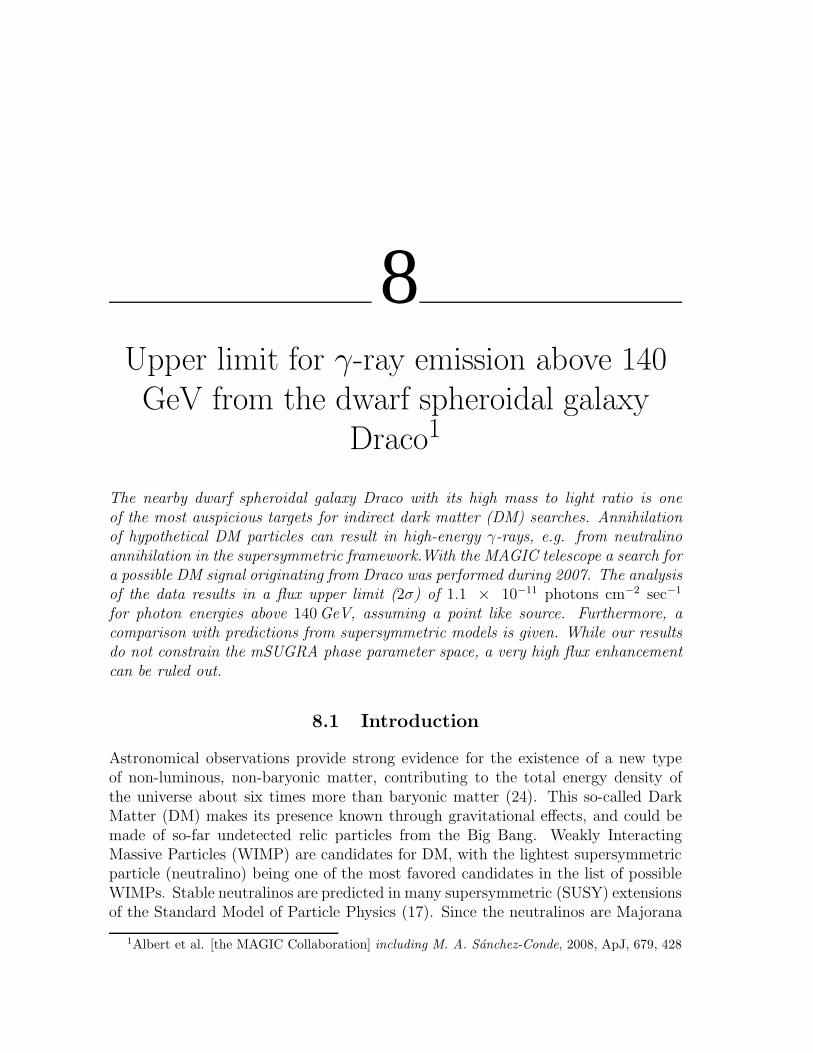
8Upper limit for γ-ray emission above 140
GeV from the dwarf spheroidal galaxy
Draco1
The nearby dwarf spheroidal galaxy Draco with its high mass to light ratio is oneof the most auspicious targets for indirect dark matter (DM) searches. Annihilationof hypothetical DM particles can result in high-energy γ-rays, e.g. from neutralinoannihilation in the supersymmetric framework.With the MAGIC telescope a search fora possible DM signal originating from Draco was performed during 2007. The analysisof the data results in a flux upper limit (2σ) of 1.1 × 10⁻¹¹ photons cm−2 sec−1
for photon energies above 140 GeV, assuming a point like source. Furthermore, acomparison with predictions from supersymmetric models is given. While our resultsdo not constrain the mSUGRA phase parameter space, a very high flux enhancementcan be ruled out.
8.1 Introduction
Astronomical observations provide strong evidence for the existence of a new typeof non-luminous, non-baryonic matter, contributing to the total energy density ofthe universe about six times more than baryonic matter (24). This so-called DarkMatter (DM) makes its presence known through gravitational effects, and could bemade of so-far undetected relic particles from the Big Bang. Weakly InteractingMassive Particles (WIMP) are candidates for DM, with the lightest supersymmetricparticle (neutralino) being one of the most favored candidates in the list of possibleWIMPs. Stable neutralinos are predicted in many supersymmetric (SUSY) extensionsof the Standard Model of Particle Physics (17). Since the neutralinos are Majorana
1Albert et al. [the MAGIC Collaboration] including M. A. Sanchez-Conde, 2008, ApJ, 679, 428
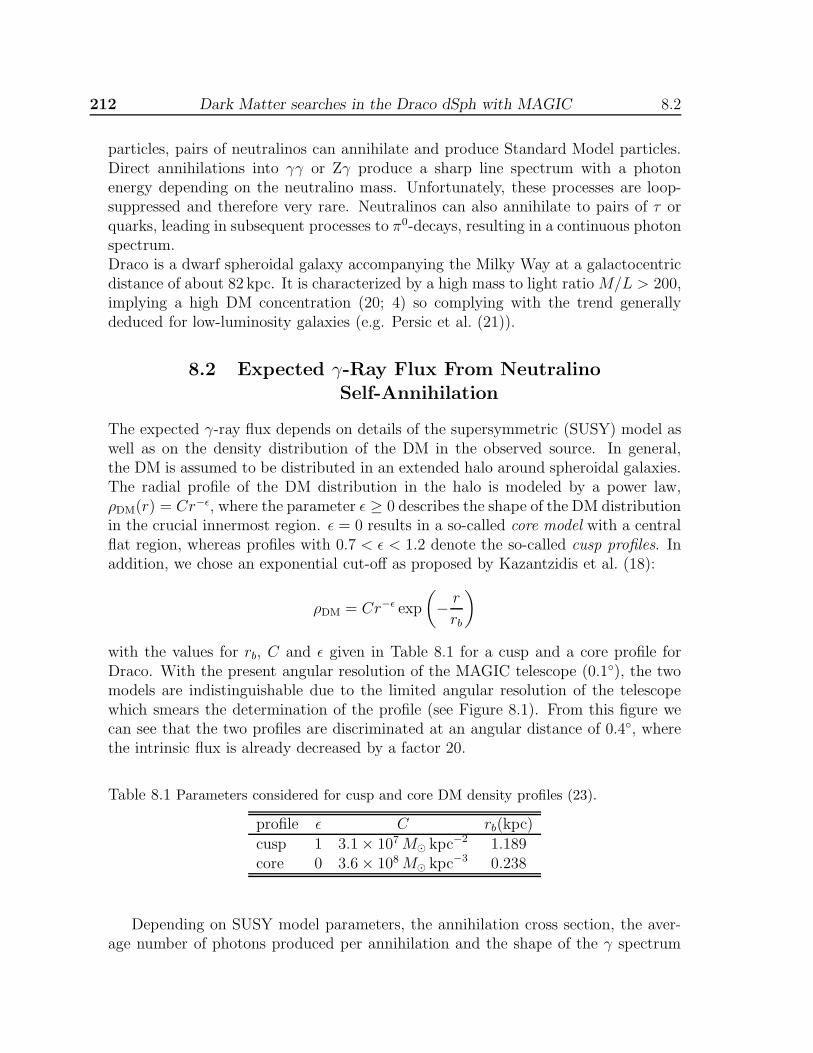
212 Dark Matter searches in the Draco dSph with MAGIC 8.2
particles, pairs of neutralinos can annihilate and produce Standard Model particles.Direct annihilations into γγ or Zγ produce a sharp line spectrum with a photonenergy depending on the neutralino mass. Unfortunately, these processes are loop-suppressed and therefore very rare. Neutralinos can also annihilate to pairs of τ orquarks, leading in subsequent processes to π0-decays, resulting in a continuous photonspectrum.Draco is a dwarf spheroidal galaxy accompanying the Milky Way at a galactocentricdistance of about 82 kpc. It is characterized by a high mass to light ratio M/L > 200,implying a high DM concentration (20; 4) so complying with the trend generallydeduced for low-luminosity galaxies (e.g. Persic et al. (21)).
8.2 Expected γ-Ray Flux From NeutralinoSelf-Annihilation
The expected γ-ray flux depends on details of the supersymmetric (SUSY) model aswell as on the density distribution of the DM in the observed source. In general,the DM is assumed to be distributed in an extended halo around spheroidal galaxies.The radial profile of the DM distribution in the halo is modeled by a power law,ρDM(r) = Cr−ǫ, where the parameter ǫ ≥ 0 describes the shape of the DM distributionin the crucial innermost region. ǫ = 0 results in a so-called core model with a centralflat region, whereas profiles with 0.7 < ǫ < 1.2 denote the so-called cusp profiles. Inaddition, we chose an exponential cut-off as proposed by Kazantzidis et al. (18):
ρDM = Cr−ǫ exp
(
− r
rb
)
with the values for rb, C and ǫ given in Table 8.1 for a cusp and a core profile forDraco. With the present angular resolution of the MAGIC telescope (0.1), the twomodels are indistinguishable due to the limited angular resolution of the telescopewhich smears the determination of the profile (see Figure 8.1). From this figure wecan see that the two profiles are discriminated at an angular distance of 0.4, wherethe intrinsic flux is already decreased by a factor 20.
Table 8.1 Parameters considered for cusp and core DM density profiles (23).
profile ǫ C rb(kpc)
cusp 1 3.1 × 10⁷M⊙ kpc−2 1.189core 0 3.6 × 10⁸M⊙ kpc−3 0.238
Depending on SUSY model parameters, the annihilation cross section, the aver-age number of photons produced per annihilation and the shape of the γ spectrum
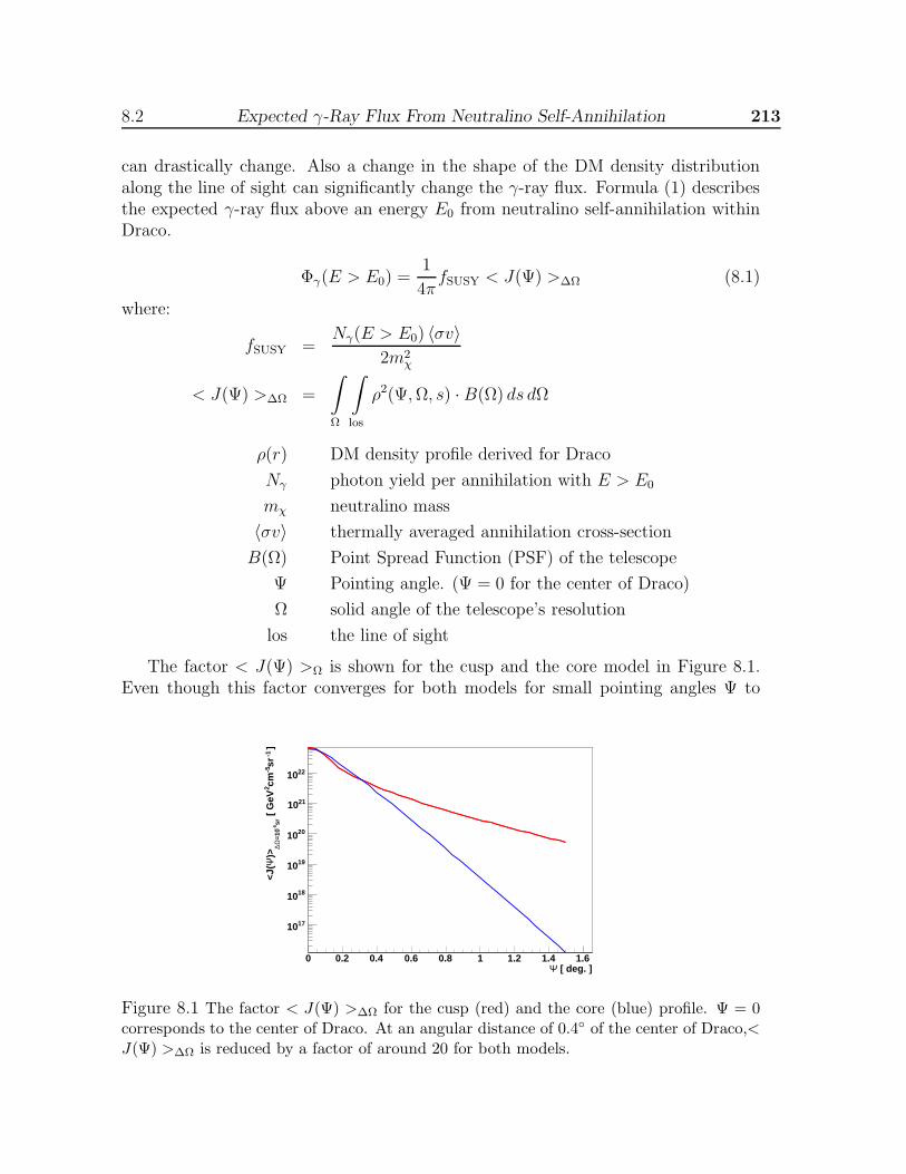
8.2 Expected γ-Ray Flux From Neutralino Self-Annihilation 213
can drastically change. Also a change in the shape of the DM density distributionalong the line of sight can significantly change the γ-ray flux. Formula (1) describesthe expected γ-ray flux above an energy E0 from neutralino self-annihilation withinDraco.
Φγ(E > E0) =1
4πfSUSY < J(Ψ) >∆Ω (8.1)
where:
fSUSY =Nγ(E > E0) 〈σv〉
2m2χ
< J(Ψ) >∆Ω =
∫
Ω
∫
los
ρ2(Ψ,Ω, s) · B(Ω) ds dΩ
ρ(r) DM density profile derived for Draco
Nγ photon yield per annihilation with E > E0
mχ neutralino mass
〈σv〉 thermally averaged annihilation cross-section
B(Ω) Point Spread Function (PSF) of the telescope
Ψ Pointing angle. (Ψ = 0 for the center of Draco)
Ω solid angle of the telescope’s resolution
los the line of sight
The factor < J(Ψ) >Ω is shown for the cusp and the core model in Figure 8.1.Even though this factor converges for both models for small pointing angles Ψ to
[ deg. ]Ψ0 0.2 0.4 0.6 0.8 1 1.2 1.4 1.6
]-1
sr-5
cm2 [
GeV
sr-5
=10
Ω∆
)>Ψ
<J(
1710
1810
1910
2010
2110
2210
Figure 8.1 The factor < J(Ψ) >∆Ω for the cusp (red) and the core (blue) profile. Ψ = 0corresponds to the center of Draco. At an angular distance of 0.4 of the center of Draco,<J(Ψ) >∆Ω is reduced by a factor of around 20 for both models.
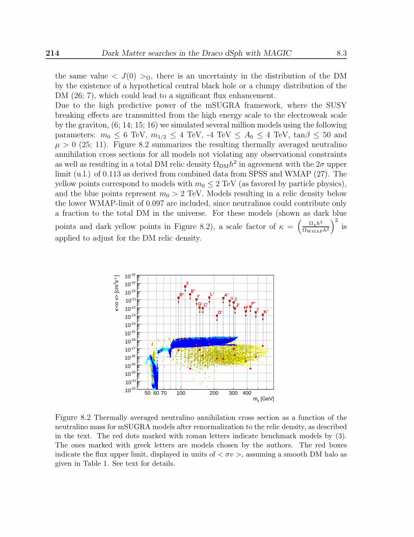
214 Dark Matter searches in the Draco dSph with MAGIC 8.3
the same value < J(0) >Ω, there is an uncertainty in the distribution of the DMby the existence of a hypothetical central black hole or a clumpy distribution of theDM (26; 7), which could lead to a significant flux enhancement.Due to the high predictive power of the mSUGRA framework, where the SUSYbreaking effects are transmitted from the high energy scale to the electroweak scaleby the graviton, (6; 14; 15; 16) we simulated several million models using the followingparameters: m0 ≤ 6 TeV, m1/2 ≤ 4 TeV, -4 TeV ≤ A0 ≤ 4 TeV, tanβ ≤ 50 andµ > 0 (25; 11). Figure 8.2 summarizes the resulting thermally averaged neutralinoannihilation cross sections for all models not violating any observational constraintsas well as resulting in a total DM relic density ΩDMh
2 in agreement with the 2σ upperlimit (u.l.) of 0.113 as derived from combined data from SPSS and WMAP (27). Theyellow points correspond to models with m0 ≤ 2 TeV (as favored by particle physics),and the blue points represent m0 > 2 TeV. Models resulting in a relic density belowthe lower WMAP-limit of 0.097 are included, since neutralinos could contribute onlya fraction to the total DM in the universe. For these models (shown as dark blue
points and dark yellow points in Figure 8.2), a scale factor of κ =(
Ωχh2
ΩWMAPh2
)2
is
applied to adjust for the DM relic density.
[GeV]χm50 60 70 100 200 300 400
]-1 s3
v>
[cm
σ<κ
-3210
-3110
-3010
-2910
-2810
-2710
-2610
-2510
-2410
-2310
-2210
-2110
-2010
-1910
-1810
A’B’
C’
D’
E’
F’G’H’
I’
J’K’
L’α β
γ
δ
Figure 8.2 Thermally averaged neutralino annihilation cross section as a function of theneutralino mass for mSUGRA models after renormalization to the relic density, as describedin the text. The red dots marked with roman letters indicate benchmark models by (3).The ones marked with greek letters are models chosen by the authors. The red boxesindicate the flux upper limit, displayed in units of < σv >, assuming a smooth DM halo asgiven in Table 1. See text for details.
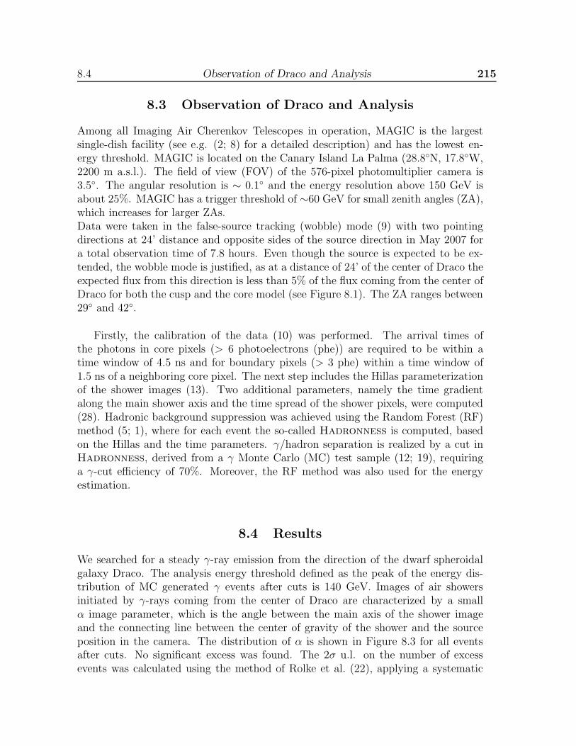
8.4 Observation of Draco and Analysis 215
8.3 Observation of Draco and Analysis
Among all Imaging Air Cherenkov Telescopes in operation, MAGIC is the largestsingle-dish facility (see e.g. (2; 8) for a detailed description) and has the lowest en-ergy threshold. MAGIC is located on the Canary Island La Palma (28.8N, 17.8W,2200 m a.s.l.). The field of view (FOV) of the 576-pixel photomultiplier camera is3.5. The angular resolution is ∼ 0.1 and the energy resolution above 150 GeV isabout 25%. MAGIC has a trigger threshold of ∼60 GeV for small zenith angles (ZA),which increases for larger ZAs.Data were taken in the false-source tracking (wobble) mode (9) with two pointingdirections at 24’ distance and opposite sides of the source direction in May 2007 fora total observation time of 7.8 hours. Even though the source is expected to be ex-tended, the wobble mode is justified, as at a distance of 24’ of the center of Draco theexpected flux from this direction is less than 5% of the flux coming from the center ofDraco for both the cusp and the core model (see Figure 8.1). The ZA ranges between29 and 42.
Firstly, the calibration of the data (10) was performed. The arrival times ofthe photons in core pixels (> 6 photoelectrons (phe)) are required to be within atime window of 4.5 ns and for boundary pixels (> 3 phe) within a time window of1.5 ns of a neighboring core pixel. The next step includes the Hillas parameterizationof the shower images (13). Two additional parameters, namely the time gradientalong the main shower axis and the time spread of the shower pixels, were computed(28). Hadronic background suppression was achieved using the Random Forest (RF)method (5; 1), where for each event the so-called Hadronness is computed, basedon the Hillas and the time parameters. γ/hadron separation is realized by a cut inHadronness, derived from a γ Monte Carlo (MC) test sample (12; 19), requiringa γ-cut efficiency of 70%. Moreover, the RF method was also used for the energyestimation.
8.4 Results
We searched for a steady γ-ray emission from the direction of the dwarf spheroidalgalaxy Draco. The analysis energy threshold defined as the peak of the energy dis-tribution of MC generated γ events after cuts is 140 GeV. Images of air showersinitiated by γ-rays coming from the center of Draco are characterized by a smallα image parameter, which is the angle between the main axis of the shower imageand the connecting line between the center of gravity of the shower and the sourceposition in the camera. The distribution of α is shown in Figure 8.3 for all eventsafter cuts. No significant excess was found. The 2σ u.l. on the number of excessevents was calculated using the method of Rolke et al. (22), applying a systematic
216 Dark Matter searches in the Draco dSph with MAGIC 8.5
]° [α0 10 20 30 40 50 60 70 80 90
entr
ies
800
900
1000
1100
1200
1300
Figure 8.3 Distribution of the α parameter for γ-ray candidates coming from the center ofDraco (black marker) and background (grey markers) for data taken between 05/09/2007- 05/20/2007. The energy threshold is 140 GeV. For the signal region (α < 12), are thenumber of ON events: 10883 and the number of OFF events: 10996. With the method of(22), the 2σ upper limit on excess events is 231.
error of 30%. The number of excess events were converted into an integral flux u.l.,depending on the assumed underlying spectrum. For a power law with spectral index−1.5, typical for a DM annihilation spectrum, and assuming a point like source, the2σ u.l. is:
Φ2σ(E > 140 GeV) = 1.1 × 10⁻¹¹ photons cm−2 s−1.
For different mSUGRA model parameters using the benchmark points defined in(3) and for other models, we computed the γ-ray spectra expected from neutralinoannihilations. Assuming these underlying spectra, the u.l. on the integrated fluxabove 140 GeV is computed. Using formula (1) and assuming a DM distributionfollowing the profiles according to Table 1, the flux u.l. is displayed in the units of athermally averaged cross section in Table 2 and in Figure 8.2:
F2σ =Φ2σ(E > E0)
Φγ(E > E0)< σv > (8.2)
As can be seen, the measured flux u.l. is several orders of magnitude larger thanpredicted for the smooth DM distribution. But a high clumpy structure of the DMdistribution or a central black hole could provide a significant flux enhancement(26; 7), which would decrease F2σ. The analysis presented here can set a limit on theflux enhancement depending on the mSUGRA input parameters. For the benchmarkmodels the values for κ < σv > and F2σ are displayed in Table 8.2 and in Figure 8.2.For these models, the u.l. on the flux enhancement is around O(103 − 109).

8.5R
esults
217
Table 8.2 Thermally averaged neutralino annihilation cross section < σv >, the u.l. on the flux F2σ, displayed in units of< σv >, and the 2σ u.l. on the flux enhancement. Models A’ - L’ correspond to the benchmark models given by (3). Models α- δ are typical models chosen by the authors with A0 6= 0.
model: A’ B’ C’ D’ E’ F’ G’ H’
m0 [GeV] 107 57 80 101 1532 3440 113 244
A0 [GeV] 0 0 0 0 0 0 0 0
m1/2 [GeV] 600 250 400 525 300 1000 375 935
tan β 5 10 10 10 10 10 20 20
mχ [GeV] 243 95 158 212 121 428 148 389
κ < σv > [cm3 s−1] 5.55 · 10−29 6.83 · 10−28 1.42 · 10−28 6.05 · 10−29 3.74 · 10−30 3.65 · 10−30 7.18 · 10−28 2.87 · 10−29
F2σ [cm3 s−1] 1.63 · 10−21 1.79 · 10−21 1.00 · 10−22 1.15 · 10−23 4.82 · 10−21 1.42 · 10−22 1.11 · 10−22 3.92 · 10−23
boost factor 2.9 · 107 2.6 · 106 7.0 · 105 1.9 · 105 1.3 · 109 3.9 · 107 1.5 · 105 1.4 · 106
model: I’ J’ K’ L’ α β γ δ
m0 [GeV] 181 299 1001 303 5980 180 1140 4540
A0 [GeV] 0 0 0 0 -300 -2800 -1800 300
m1/2 [GeV] 350 750 1300 450 680 720 1120 300
tan β 35 35 46 47 50 5 50 35
mχ [GeV] 138 309 554 181 277 301 479 109
κ < σv > [cm3 s−1] 3.17 · 10−27 1.67 · 10−28 2.22 · 10−27 3.85 · 10−27 2.27 · 10−26 9.75 · 10−28 9.43 · 10−29 1.79 · 10−26
F2σ [cm3 s−1] 1.08 · 10−21 9.02 · 10−23 1.44 · 10−23 1.91 · 10−21 7.22 · 10−22 4.78 · 10−22 2.97 · 10−23 4.39 · 10−20
boost factor 3.4 · 105 5.4 · 105 6.5 · 103 4.9 · 105 3.2 · 104 4.9 · 105 3.1 · 105 2.4 · 106

218 Dark Matter searches in the Draco dSph with MAGIC 8.5
8.5 Conclusions
We present the first search for γ-rays from the direction of Draco using an Imag-ing Air Cherenkov Telescope (IACT). No signal was detected. The 2σ u.l. ona steady γ-ray emission above 140 GeV originating from Draco does not exceed1.1 × 10−11 photons cm−2 s−1 if the underlying spectrum follows a power law withspectral index -1.5.For the mSUGRA benchmark models defined in (3) and assuming a smooth DMdensity distribution for Draco as given in (23), our flux upper limits are O(103 - 109)above the predicted values. It is therefore not possible to constrain the mSUGRAphase space by these results, but a very high flux enhancement can be excluded.Even though an indirect DM detection by measuring γ-rays from neutralino annihi-lation within the halo of Draco seems for present IACTs out of reach, future satellitetelescopes like GLAST with lower energy thresholds might be sensitive enough toreach the mSUGRA parameter space.

Bibliography
Albert, J. et al. 2007, astro-ph/0709.3719
Baixeras, C. et al. 2004, Nucl. Instrum. Meth., A518, 188
Battaglia, M. et al. 2004, Eur. Phys. J., C33, 273
Bergstrom, L. & Hooper, D. 2006, Phys. Rev. D, 73, 063510
Breiman, L. 2001, Machine Learning, 45, 5
Chamseddine, A. H., Arnowitt, R., & Nath, P. 1982, Phys. Rev. Lett., 49, 970
Colafrancesco, S., Profumo, S., & Ullio, P. 2007, Phys. Rev. D, 75, 023513
Cortina, J. et al. 2005, 5, 359, proc. of the 29th ICRC, Pune, India
Fomin, V. P., Stepanian, A., A., Lamb, R. C., Lewis, D. A., Punch, M., & Weekes,T. C. 1994, Astroparticle Physics, 2, 137
Gaug, M. 2005, proc. of the 7th Workshop on Towards a Network of AtmosphericCherenkov Detectors 2005, Palaiseau, France, 27-29 Apr 2005
Gondolo, P., Edsjo, J., Bergstrom, L., Ullio, P., & Baltz, E. A. 2000, astro-ph/0012234
Heck, D., Schatz, G., Thouw, T., Knapp, J., & Capdevielle, J. N. 1998, fZKA-6019
Hillas, A. M. 1985, proc. of the 19th ICRC, La Jolla, 3, 445
Inoue, K., Kakuto, A., Komatsu, H., & Takeshita, S. 1982, Prog. Theor. Phys., 68,927
—. 1982, Prog. Theor. Phys., 67, 1889
—. 1984, Prog. Theor. Phys., 71, 413
Jungman, G. & Kamionkowski, M. 1995, Phys. Rev. D, 51, 3121
220 BIBLIOGRAPHY 8.5
Kazantzidis, S., Mayer, L., Mastropietro, C., Diemand, J., Stadel, J., & Moore, B.2004, ApJ, 608, 663
Majumdar, P., Moralejo, A., Bigongiari, C., Blanch, O., & Sobczynska, D. 2005,5, 203, proc. of the 29th International Cosmic Ray Conference (ICRC 2005), Pune,India, 3-11 Aug 2005
Mayer, L., Kazantzidis, S., Mastropietro, C., & Wadsley, J. 2007, Nature, 445, 738
Persic, M., Salucci, P., & Stel, F. 1996, MNRAS, 281, 27
Rolke, W. A., Lopez, A. M., & Conrad, J. 2005, Nucl. Instrum. and Meth., A551,493
Sanchez-Conde, M. A. et al. 2007, Phys. Rev. D 76, 123509
Spergel, D. N., Bean, R., Dore, O., Nolta, M. R., Bennett, C. L., Dunkley, J.,Hinshaw, G., Jarosik, N., Komatsu, E., Page, L., Peiris, H. V., Verde, L., Halpern,M., Hill, R. S., Kogut, A., Limon, M., Meyer, S. S., Odegard, N., Tucker, G. S.,Weiland, J. L., Wollack, E., & Wright, E. L. 2007, ApJS, 170, 377
Stark, L. S., Hafliger, P., Biland, A., & Pauss, F. 2005, JHEP, 08, 059
Strigari, L. E., Koushiappas, S. M., Bullock, J. S., & Kaplinghat, M. 2007,Phys. Rev. D, 75, 083526
Tegmark, M. et al. 2006, Phys. Rev. D, 74, 123507
Tescaro, D. et al. 2007, proc. of the 30th ICRC, Merida, Mexico

9MAGIC upper limits on the VHE
gamma–ray emission from the Willman 1
satellite galaxy1
We present the result of the observation of the ultra–faint dwarf galaxy Willman 1performed with the 17 m MAGIC Cherenkov telescope during 15.5 hours betweenMarch and May 2008. No significant gamma–ray emission was found above 100 GeV.We derived upper limits of the order of 10−12 ph cm−2 s−1 on the integral flux above100 GeV, which we compare with predictions from several of the established neutralinobenchmark models in the mSUGRA parameter space. The neutralino annihilationspectra are defined after including the recently discovered contribution of internalbremsstrahlung from the virtual sparticles that mediate the annihilation. Flux boostfactors of three orders of magnitude are required even in the most optimistic scenarioto match our upper limits. However, uncertainties in the DM distribution (e.g.,presence of substructure in the halo) may significantly reduce such boost estimates.Future observations will likely allow us to improve the derived upper limits probablyby up to one order of magnitude so that — at least in some regions — the mSUGRAparameter space may be constrained.
9.1 Introduction
Dwarf Spheroidal Galaxies (dSph) are believed to be the smallest (size 1 ∼ kpc),faintest (luminosities 102 − 108 L⊙) astronomical objects whose dynamics are domi-nated by dark matter (DM) (Gilmore et al. 2007 and references therein). They arefound as satellites orbiting in the gravitational field of a larger host galaxy (e.g., the
1Aliu et al. [the MAGIC Collaboration] (corresponding authors: M. Doro and M. A. Sanchez-Conde), 2009, ApJ, 697, 1299
222 Dark Matter searches in the Willman 1 dSph with MAGIC 9.1
Milky Way (MW)). Usually, their member stars show large circular velocities and ve-locity dispersions that, combined with their modest spatial extent, can be interpretedby the presence of a large DM halo of the order of 105 − 108 M⊙. In recent years theSloan Digital Sky Survey (SDSS) (York et al. 2000) led to the discovery of a newpopulation of MW satellites, comprising about as many (new) objects as were previ-ously known (Willman et al. 2005a; Zucker et al. 2006; Irwin et al. 2007; Walsh et al.2007; Belokurov et al. 2007). This population of extremely low–luminosity galaxiescan be very interesting for DM searches and for investigating galaxy formation atthe lowest mass scales. The existence of a new class of ultra–faint MW satellites isalso relevant because it provides a partial solution for the so-called “missing satelliteproblem” (Klypin et al. 1999; Simon & Geha 2007; Strigari et al. 2007; Madau et al.2008) by partially filling the gap between the predicted and the measured number ofgalactic sub-halos. In this family is Willman 1, discovered by Willman et al. (2005a)and soon established as potentially the most DM dominated dSph satellite of theMW (Martin et al. 2007; Sanchez-Salcedo & Hernandez 2007; Strigari et al. 2008).
The physics of DM has gathered much interest in recent years, in particular af-ter WMAP (Spergel et al. 2006; Komatsu et al. 2008) measured its relic densitywith great precision. It is generally believed that DM manifests itself as a generalclass of weakly–interacting massive particles that includes several candidates whichsatisfy both experimental constraints and theoretical requirements (see Bertone etal. 2005a and reference therein). Among them, one of the best theoretically moti-vated, for whom the relic density is calculated without fine–tuning from its nature,is the neutralino, arising in Super–Symmetric (SUSY) theories beyond the Stan-dard Model (Wess et al. 1974; Haber & Kane 1984) and in particular the mSUGRASUSY–extension (Chamseddine et al. 1982). The mSUGRA neutralino annihilationscan be observed through the production of γ−rays. The main emission comes fromsecondary products of hadronization processes and from final state radiation. Inaddition, line emissions are found through direct processes such as χχ → γγ, andχχ→ Z0γ, which provide γ−rays of energies E = mχ and E = mχ−m2
Z0/m2χ respec-
tively, even if these lines are normally strongly suppressed compared to broad–bandemission.
Recently Bringmann et al. (2008a), following an earlier idea from Bergstrom(1989), showed that in some regions of the mSUGRA parameter space, a hithertoneglected contribution to γ−ray emission comes directly from charged sparticles me-diating the annihilation into leptons, in processes like χχ → l+l−γ. They definedthis intermediate state radiation as internal bremsstrahlung (IB). The IB mecha-nism permits to restore the helicity balance in processes that would otherwise bestrongly forbidden, and supplies γ−rays towards high energies (E > 0.6 mχ) of upto several orders of magnitude. This boosted emission is particularly interesting forground–based γ−ray observation, as performed by Imaging Atmospheric CherenkovTelescopes (IACTs), which are usually sensitive above ∼ 100 GeV where normallythe IB boost takes place.
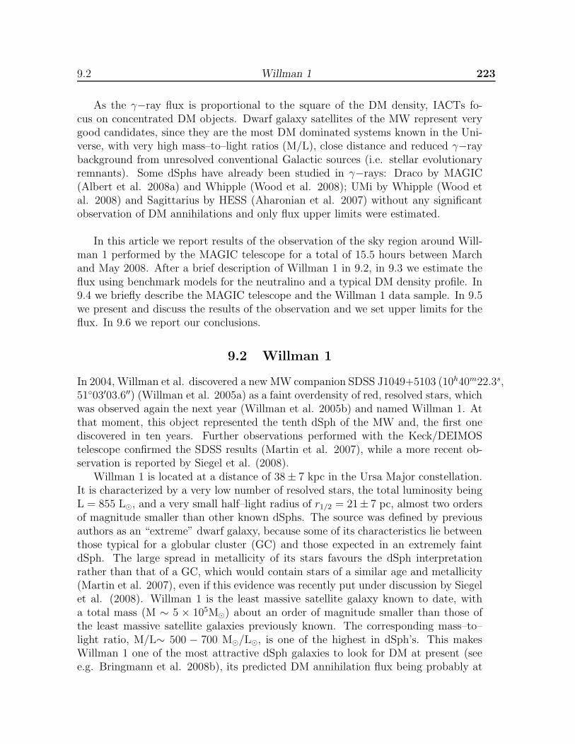
9.2 Willman 1 223
As the γ−ray flux is proportional to the square of the DM density, IACTs fo-cus on concentrated DM objects. Dwarf galaxy satellites of the MW represent verygood candidates, since they are the most DM dominated systems known in the Uni-verse, with very high mass–to–light ratios (M/L), close distance and reduced γ−raybackground from unresolved conventional Galactic sources (i.e. stellar evolutionaryremnants). Some dSphs have already been studied in γ−rays: Draco by MAGIC(Albert et al. 2008a) and Whipple (Wood et al. 2008); UMi by Whipple (Wood etal. 2008) and Sagittarius by HESS (Aharonian et al. 2007) without any significantobservation of DM annihilations and only flux upper limits were estimated.
In this article we report results of the observation of the sky region around Will-man 1 performed by the MAGIC telescope for a total of 15.5 hours between Marchand May 2008. After a brief description of Willman 1 in 9.2, in 9.3 we estimate theflux using benchmark models for the neutralino and a typical DM density profile. In9.4 we briefly describe the MAGIC telescope and the Willman 1 data sample. In 9.5we present and discuss the results of the observation and we set upper limits for theflux. In 9.6 we report our conclusions.
9.2 Willman 1
In 2004, Willman et al. discovered a new MW companion SDSS J1049+5103 (10h40m22.3s,5103′03.6′′) (Willman et al. 2005a) as a faint overdensity of red, resolved stars, whichwas observed again the next year (Willman et al. 2005b) and named Willman 1. Atthat moment, this object represented the tenth dSph of the MW and, the first onediscovered in ten years. Further observations performed with the Keck/DEIMOStelescope confirmed the SDSS results (Martin et al. 2007), while a more recent ob-servation is reported by Siegel et al. (2008).
Willman 1 is located at a distance of 38 ± 7 kpc in the Ursa Major constellation.It is characterized by a very low number of resolved stars, the total luminosity beingL = 855 L⊙, and a very small half–light radius of r1/2 = 21± 7 pc, almost two ordersof magnitude smaller than other known dSphs. The source was defined by previousauthors as an “extreme” dwarf galaxy, because some of its characteristics lie betweenthose typical for a globular cluster (GC) and those expected in an extremely faintdSph. The large spread in metallicity of its stars favours the dSph interpretationrather than that of a GC, which would contain stars of a similar age and metallicity(Martin et al. 2007), even if this evidence was recently put under discussion by Siegelet al. (2008). Willman 1 is the least massive satellite galaxy known to date, witha total mass (M ∼ 5 × 10⁵M⊙) about an order of magnitude smaller than those ofthe least massive satellite galaxies previously known. The corresponding mass–to–light ratio, M/L∼ 500 − 700 M⊙/L⊙, is one of the highest in dSph’s. This makesWillman 1 one of the most attractive dSph galaxies to look for DM at present (seee.g. Bringmann et al. 2008b), its predicted DM annihilation flux being probably at

224 Dark Matter searches in the Willman 1 dSph with MAGIC 9.3
least a factor of 3 larger than the second best DM candidate, according to recentwork (Strigari et al. 2007).
9.3 Theoretical modeling of the gamma-ray emission from
Willman 1
The γ−ray flux originating from DM particle annihilations can be factorized into acontribution called the astrophysical factor J(Ψ) related to the morphology of theemission region and a contribution called the particle physics factor ΦPP dependingon the candidate particle characteristics:
Φ(> E0) = J(Ψ) · ΦPP (> E0) , (9.1)
where E0 is the energy threshold of the detector and Ψ the angle under which theobservation is performed.
9.3.1 Astrophysical Factor
At present, a concise and exact characterization of the DM density profile of Will-man 1 is a delicate task, since observational data are still scarce. This paper is basedon the modeling from Strigari et al. (2008), who modeled the profile by using only 47stars after removing those with unclear kinematics. Furthermore, to avoid member-ship problems, only the observational data related to the inner half of the galaxy weretaken into account. It is important to note that a null/insignificant tidal–strippingwas assumed in order to carry out the modeling of the DM distribution as a systemin dynamical equilibrium, a fact which is still under debate. For example, Willmanet al. (2006) claim the existence of strong tidal debris, the evolution of the dwarfbeing strongly affected by tidal interactions with the MW still now, although DMconstitutes 90% of its total mass. In the same line, Martin et al. (2007), followingdeep observations in the r-band, infer that Willman 1 may probably be surroundedby tidal tails. The authors give as a plausible scenario that the dwarf could havebeen significantly tidally stripped but only in the past, when the object was moreluminous and massive. At that age, Willman 1 could have lost most of its outskirts,only the innermost regions surviving intact. This picture would then allow the twocontradictory arguments to coexist, since at least a correct modeling for the core ofthe dwarf may be possible assuming this region to be in dynamical equilibrium.
A very common modeling of the DM distribution, and the only one so far appliedto Willman 1 (Strigari et al. 2008), is the NFW DM density profile (Navarro et al.1996):
ρNFW(r) = ρs
(
r
rs
)−1(
1 +r
rs
)−2
, (9.2)

9.3 Theoretical modeling of the gamma-ray emission from Willman 1 225
where ρs and rs are a typical scale density and radius respectively. The astrophysicalfactor can be written as:
J(Ψ0) =1
4 π
∫
V
dΩ
∫
l.o.s
dλ [ρ2(r) ∗Bϑr(θ)] , (9.3)
where Ψ0 denoted the direction of the target. The first integral is performed overthe spatial extension of the source, the second is performed over the line of sightvariable λ. The density is convoluted with the Gaussian function Bϑr
(θ) describingthe telescope angular resolution where θ = Ψ−Ψ0 is the angular distance with respectto the center of the object. We remark that the integration of 9.3 involves foreground(MW halo) and extragalactic background whose contributions can be substantial(Elsaesser & Mannheim 2004).
At a distance of 38 kpc, the scale radius corresponds to an extension of 0.54 inthe sky, which is well inside the MAGIC field of view (∼ 3.5), but is rather extendedif one considers that the telescope angular resolution is around 0.1. This evidenceis mitigated by the fact that the main emission still comes from the very core ofthe source, due to the very steep NFW profile at the center and the square densitydependence. For this reason, we performed an analysis adapted for just slightlyextended sources (Sitarek & Mirzoyan 2008). To compute the astrophysical factor forWillman 1, we substitute rs = 0.18 kpc and ρs = 4×10⁸ M⊙/kpc3 taken from Strigariet al. (2008) into 9.2, and by computing 9.3 we obtain J(Ψ0) ∼ 3.5×10¹⁷ GeV2/cm5.As already commented, this value for the DM annihilation flux probably representsthe largest over the rest of dwarfs.
9.3.2 Particle Physics Factor
In many mSUGRA models, the lightest supersymmetric particle is one of four neu-tralinos (χ0
1...4) which are linear combinations of the Bino B0, the Wino W 0 and the
two neutral higgsinos H0u, H
0d . Only five free parameters fully characterize mSUGRA:
the scalar mass m0 and the gaugino mass m1/2 defined at the unification scale, thetrilinear scalar coupling A0 and the ratio tan β of the Higgs vacuum expectation val-ues. In addition, one needs to define the sign of the Higgs mass parameter sign(µ).The typical DM γ−ray annihilation spectrum is a power–law with a sharp cutoff atthe DM candidate’s mass, and with a possible bump at energies larger than 0.6 mχ incase the IB is present, see 9.1. WMAP relic density measurements provide an upperlimit in the total neutralino cross section of order of 〈σv〉 ∼ 10−26 cm3s−1 (Bertone etal. 2005b), which implies that the neutralino is an extremely low–interacting particleand thus the expected γ−ray flux is correspondingly low today.
The particle physics factor can be written as a product of two terms, the firstdepending only on the DM candidate’s mass and cross section, and a second term,depending on the annihilation γ−ray spectra, which must be integrated above the
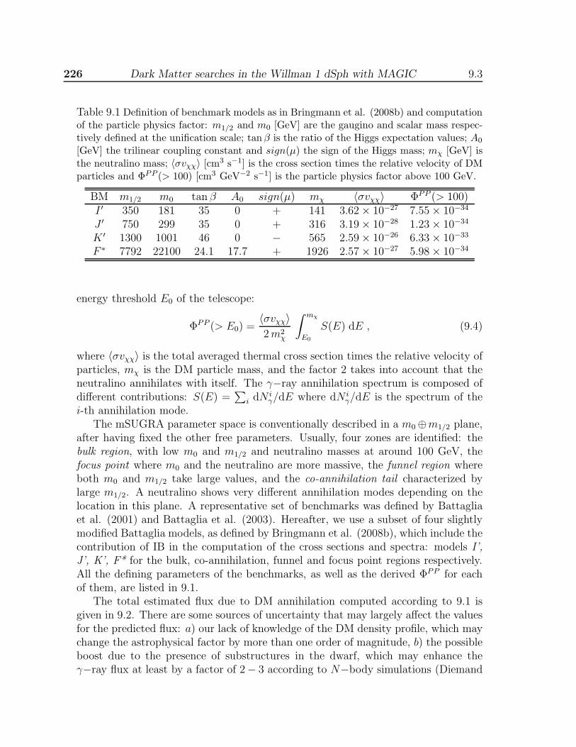
226 Dark Matter searches in the Willman 1 dSph with MAGIC 9.3
Table 9.1 Definition of benchmark models as in Bringmann et al. (2008b) and computationof the particle physics factor: m1/2 and m0 [GeV] are the gaugino and scalar mass respec-tively defined at the unification scale; tan β is the ratio of the Higgs expectation values; A0
[GeV] the trilinear coupling constant and sign(µ) the sign of the Higgs mass; mχ [GeV] isthe neutralino mass; 〈σvχχ〉 [cm3 s−1] is the cross section times the relative velocity of DMparticles and ΦPP (> 100) [cm3 GeV−2 s−1] is the particle physics factor above 100 GeV.
BM m1/2 m0 tan β A0 sign(µ) mχ 〈σvχχ〉 ΦPP (> 100)I ′ 350 181 35 0 + 141 3.62 × 10⁻²⁷ 7.55 × 10⁻³⁴
J ′ 750 299 35 0 + 316 3.19 × 10⁻²⁸ 1.23 × 10⁻³⁴
K ′ 1300 1001 46 0 − 565 2.59 × 10⁻²⁶ 6.33 × 10−33
F ∗ 7792 22100 24.1 17.7 + 1926 2.57 × 10⁻²⁷ 5.98 × 10⁻³⁴
energy threshold E0 of the telescope:
ΦPP (> E0) =〈σvχχ〉2m2
χ
∫ mχ
E0
S(E) dE , (9.4)
where 〈σvχχ〉 is the total averaged thermal cross section times the relative velocity ofparticles, mχ is the DM particle mass, and the factor 2 takes into account that theneutralino annihilates with itself. The γ−ray annihilation spectrum is composed ofdifferent contributions: S(E) =
∑
i dN iγ/dE where dN i
γ/dE is the spectrum of thei-th annihilation mode.
The mSUGRA parameter space is conventionally described in a m0 ⊕m1/2 plane,after having fixed the other free parameters. Usually, four zones are identified: thebulk region, with low m0 and m1/2 and neutralino masses at around 100 GeV, thefocus point where m0 and the neutralino are more massive, the funnel region whereboth m0 and m1/2 take large values, and the co-annihilation tail characterized bylarge m1/2. A neutralino shows very different annihilation modes depending on thelocation in this plane. A representative set of benchmarks was defined by Battagliaet al. (2001) and Battaglia et al. (2003). Hereafter, we use a subset of four slightlymodified Battaglia models, as defined by Bringmann et al. (2008b), which include thecontribution of IB in the computation of the cross sections and spectra: models I’,J’, K’, F* for the bulk, co-annihilation, funnel and focus point regions respectively.All the defining parameters of the benchmarks, as well as the derived ΦPP for eachof them, are listed in 9.1.
The total estimated flux due to DM annihilation computed according to 9.1 isgiven in 9.2. There are some sources of uncertainty that may largely affect the valuesfor the predicted flux: a) our lack of knowledge of the DM density profile, which maychange the astrophysical factor by more than one order of magnitude, b) the possibleboost due to the presence of substructures in the dwarf, which may enhance theγ−ray flux at least by a factor of 2 − 3 according to N−body simulations (Diemand
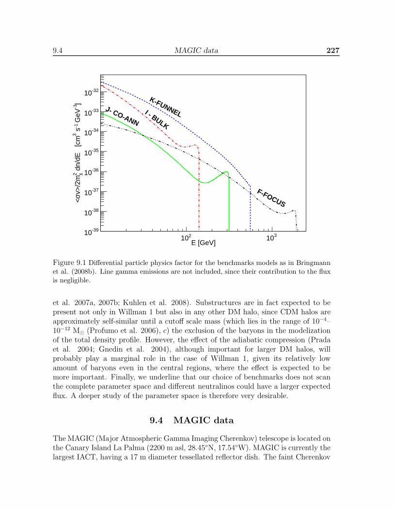
9.4 MAGIC data 227
E [GeV]210 310
]-1
GeV
-1 s
3 d
n/dE
[c
m2 χ
v>/2
mσ<
-3910
-3810
-3710
-3610
-3510
-3410
-3310
-3210K-FUNNELI - BULK
J- CO-ANN
F-FOCUS
Figure 9.1 Differential particle physics factor for the benchmarks models as in Bringmannet al. (2008b). Line gamma emissions are not included, since their contribution to the fluxis negligible.
et al. 2007a, 2007b; Kuhlen et al. 2008). Substructures are in fact expected to bepresent not only in Willman 1 but also in any other DM halo, since CDM halos areapproximately self-similar until a cutoff scale mass (which lies in the range of 10−4–10−12 M⊙ (Profumo et al. 2006), c) the exclusion of the baryons in the modelizationof the total density profile. However, the effect of the adiabatic compression (Pradaet al. 2004; Gnedin et al. 2004), although important for larger DM halos, willprobably play a marginal role in the case of Willman 1, given its relatively lowamount of baryons even in the central regions, where the effect is expected to bemore important. Finally, we underline that our choice of benchmarks does not scanthe complete parameter space and different neutralinos could have a larger expectedflux. A deeper study of the parameter space is therefore very desirable.
9.4 MAGIC data
The MAGIC (Major Atmospheric Gamma Imaging Cherenkov) telescope is located onthe Canary Island La Palma (2200 m asl, 28.45N, 17.54W). MAGIC is currently thelargest IACT, having a 17 m diameter tessellated reflector dish. The faint Cherenkov

228 Dark Matter searches in the Willman 1 dSph with MAGIC 9.5
light flashes produced by air showers initiated by VHE γ−rays in the top atmosphereare recorded by the telescope camera, which consists of 577 photomultiplier tubes.More details can be found in Cortina et al. (2005).
MAGIC observed Willman 1 between March and May 2008. The source wassurveyed at zenith angles between 22 and 30, which guarantees the lowest energythreshold. The source was surveyed for 16.8 hours plus another 9.3 hours in OFFobservation mode, i.e. pointing to a dark patch in the sky close to Willman 1 whereno γ−ray emission is expected, to estimate the background. The main backgroundCherenkov telescopes have to deal with is produced by cosmic hadronic particlesimpinging on the atmosphere and generating electromagnetic sub–showers that canmimic pure γ−rays showers, and by the night sky background. Background eventsare partly rejected at the trigger level and in the later off–line analysis event selectionfollowing a procedure called gamma/hadron (g/h) separation.
The analysis proceeds as follows (for a detailed description see Albert et al.2008b): data are calibrated and the number of photoelectrons per pixel extracted(Albert et al. 2008c), then an image cleaning selects pixels with at least 6 photoelec-trons (3 photoelectrons for pixels in the boundary of the image). Additional suppres-sion of pixels containing noise is achieved by requesting a narrow time coincidencebetween adjacent pixels (∼ 7 ns). Based on the Hillas parameterization algorithm(Hillas 1985), the shower parameters are reconstructed. The hadronic background issuppressed with a multivariate method, the Random Forest (Breiman 2001; Albertet al. 2008d), that uses the Hillas parameters to define an estimator called hadron-ness by comparison with Monte Carlo (MC) γ−ray simulations. The hadronnessexpresses the likeness of an event to be a hadron and runs from 0 for gammas to 1for hadrons. The Random Forest method is also used to estimate the energy of areconstructed shower: the energy threshold is defined by the peak of the distributionof reconstructed MC gamma events. The g/h separation is optimized on a real datasample from the Crab Nebula, a Supernova Remnant and one of the brightest andstable γ−ray emitters, which is taken as standard candle in very high energy γ−rayastronomy. The optimization yields a best set of cuts in the Hillas parameters whichdefines the gamma and hadron acceptance of the analysis. In our case, the optimalset of cuts is obtained for an energy threshold of 100 GeV and a hadronness cut of0.15. The overall data quality is very high, with only 7% data rejection, resulting in15.5 hours effective observation time. Independent cross–checks were performed onthe data giving compatible results.
9.5 Results and Discussion
No significant γ−ray excess beyond 100 GeV above the background was observed in15.5 hours of observation of the sky region around Willman 1. This is also shownin 9.2, where the “α–plot” is reported. The α–parameter is the angular distancebetween the shower image main axis and the line connecting the image barycenter
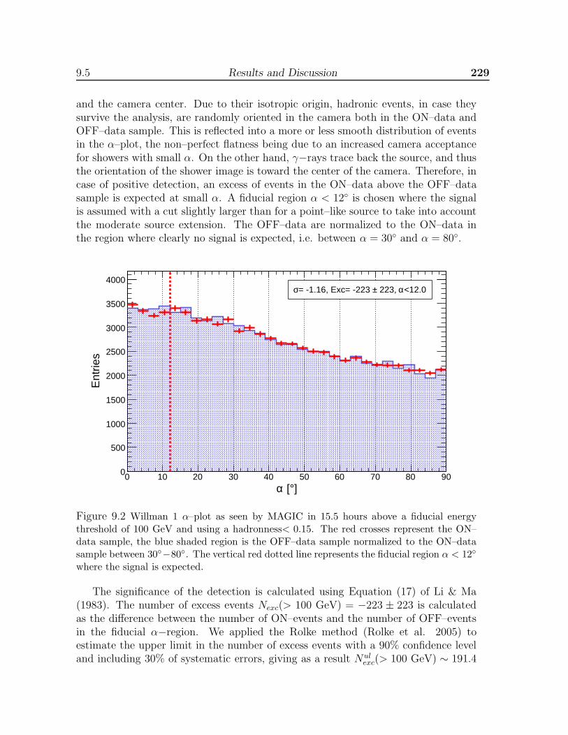
9.5 Results and Discussion 229
and the camera center. Due to their isotropic origin, hadronic events, in case theysurvive the analysis, are randomly oriented in the camera both in the ON–data andOFF–data sample. This is reflected into a more or less smooth distribution of eventsin the α–plot, the non–perfect flatness being due to an increased camera acceptancefor showers with small α. On the other hand, γ−rays trace back the source, and thusthe orientation of the shower image is toward the center of the camera. Therefore, incase of positive detection, an excess of events in the ON–data above the OFF–datasample is expected at small α. A fiducial region α < 12 is chosen where the signalis assumed with a cut slightly larger than for a point–like source to take into accountthe moderate source extension. The OFF–data are normalized to the ON–data inthe region where clearly no signal is expected, i.e. between α = 30 and α = 80.
]° [α0 10 20 30 40 50 60 70 80 90
Ent
ries
0
500
1000
1500
2000
2500
3000
3500
4000<12.0α 223, ±= -1.16, Exc= -223 σ
Figure 9.2 Willman 1 α–plot as seen by MAGIC in 15.5 hours above a fiducial energythreshold of 100 GeV and using a hadronness< 0.15. The red crosses represent the ON–data sample, the blue shaded region is the OFF–data sample normalized to the ON–datasample between 30−80. The vertical red dotted line represents the fiducial region α < 12
where the signal is expected.
The significance of the detection is calculated using Equation (17) of Li & Ma(1983). The number of excess events Nexc(> 100 GeV) = −223 ± 223 is calculatedas the difference between the number of ON–events and the number of OFF–eventsin the fiducial α−region. We applied the Rolke method (Rolke et al. 2005) toestimate the upper limit in the number of excess events with a 90% confidence leveland including 30% of systematic errors, giving as a result Nul
exc(> 100 GeV) ∼ 191.4
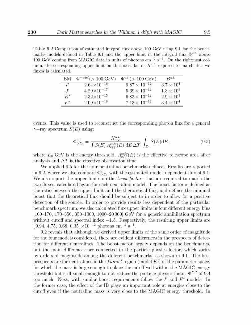
230 Dark Matter searches in the Willman 1 dSph with MAGIC 9.5
Table 9.2 Comparison of estimated integral flux above 100 GeV using 9.1 for the bench-marks models defined in Table 9.1 and the upper limit in the integral flux Φu.l. above100 GeV coming from MAGIC data in units of photons cm−2 s−1. On the rightmost col-umn, the corresponding upper limit on the boost factor Bu.l. required to match the twofluxes is calculated.
BM Φmodel(> 100 GeV) Φu.l.(> 100 GeV) Bu.l.
I ′ 2.64×10⁻¹⁶ 9.87 × 10⁻¹² 3.7 × 10⁴
J ′ 4.29×10⁻¹⁷ 5.69 × 10⁻¹² 1.3 × 10⁵
K ′ 2.32×10⁻¹⁵ 6.83 × 10⁻¹² 2.9 × 103
F ∗ 2.09×10−16 7.13 × 10⁻¹² 3.4 × 10⁴
events. This value is used to reconstruct the corresponding photon flux for a generalγ−ray spectrum S(E) using:
Φu.l.>E0
=Nu.l.
exc∫
S(E)Acutseff (E) dE∆T
∫
E0
S(E)dE , (9.5)
where E0 GeV is the energy threshold, Acutseff (E) is the effective telescope area after
analysis and ∆T is the effective observation time.We applied 9.5 for the four neutralino benchmarks defined. Results are reported
in 9.2, where we also compare Φu.l.>E0
with the estimated model–dependent flux of 9.1.We also report the upper limits on the boost factors that are required to match thetwo fluxes, calculated again for each neutralino model. The boost factor is defined asthe ratio between the upper limit and the theroretical flux, and defines the minimalboost that the theoretical flux should be subject to in order to allow for a positivedetection of the source. In order to provide results less dependent of the particularbenchmark spectrum, we also calculated flux upper limits in four different energy bins[100–170, 170–350, 350–1000, 1000–20 000] GeV for a generic annihilation spectrumwithout cutoff and spectral index −1.5. Respectively, the resulting upper limits are[ 9.94, 4.75, 0.68, 0.35 ]×10−12 photons cm−2 s−1.
9.2 reveals that although we derived upper limits of the same order of magnitudefor the four models considered, there are evident differences in the prospects of detec-tion for different neutralinos. The boost factor largely depends on the benchmarks,but the main differences are connected to the particle physics factor, which variesby orders of magnitude among the different benchmarks, as shown in 9.1. The bestprospects are for neutralinos in the funnel region (model K ′) of the parameter space,for which the mass is large enough to place the cutoff well within the MAGIC energythreshold but still small enough to not reduce the particle physics factor ΦPP of 9.4too much. Next, with similar boost requirements follow the I ′ and F ∗ models. Inthe former case, the effect of the IB plays an important role at energies close to thecutoff even if the neutralino mass is very close to the MAGIC energy threshold. In
9.6 Conclusion 231
the latter case, although the IB effect is negligible, the signal is very extended in theenergy region suitable for MAGIC, whereas the large mass makes the flux suppres-sion too large. The worst case scenario is the co–annihilation neutralino. In this case,even if the IB contribution is large, the intrinsic total cross section is very low, whichmakes the flux very low compared to the others. The IB effect cannot counteract thisintrinsic deficit.
Although the results of 9.2 seem to show that we could still be far from DMdetection (the most promising scenario being three orders of magnitude below oursensitivity), we should keep in mind that there are important uncertainties in ourmodeling that may play a crucial role in detectability issues, as already discussed in9.3.2. In particular our imperfect knowledge of the exact DM density profile as wellas the presence of substructure in the dwarf, which is theoretically well–motivated,may increase the astrophysical factor and therefore the flux of more than one order ofmagnitude. Furthermore, since the parameter space was not fully scanned, it is likelythat there are models of neutralino with higher ΦPP . The use of a more advanceddetector like MAGIC II, with increased sensitivity and lower energy threshold, favourspossible scenarios of DM detection or at least of exclusion of relevant parts of themSUGRA paparemeter space. Nonetheless, while all other current IACTs can onlycover SUSY models with a large IB contribution due to their higher energy threshold,MAGIC II will explore a much larger region of DM annihilation models where thepeak of the emission is at lower energy.
9.6 Conclusion
In the context of DM searches, we have observed the Willman 1 dwarf galaxy with theMAGIC telescope for a total of 15.5 hours between March and May 2008. Willman1 represents one of the best DM dominated systems known in the Universe to searchfor DM at present, according to its inferred dynamical properties and distance. Noγ−ray signal was detected above an energy threshold of 100 GeV. We have obtaineddifferent flux upper limits of the order of 10−12 ph cm−2 s−1 for four benchmarkmodels considered in the framework of mSUGRA.
Using the latest estimations of its structural parameters to build the DM densityprofile as well as the inclusion of the recently proposed IB mechanism, we calculatedthe boost factors needed to match the expected flux values from DM annihilation inWillman 1 with the upper limits obtained from the data. We can see that boostsin flux in the order of 103 are required in the most optimistic scenario considered.However, uncertainties in the DM distribution, the role of DM substructure or/anda different choice of the neutralino model may reduce this boost significantly. Itis expected that deeper observations of the Willman 1 dSph with the upcomingMAGIC II telescope will allow us to improve the flux limits presented here by afactor 2 − 10.
Bibliography
Aharonian F et al. 2007 Astrop. Phys. 29 55
Albert J et al. 2008a Astrop. J. 679 428
Albert J et al. 2008b Astrop. J. 674 1037
Albert J et al. 2008c Nucl. Instrum. MethodsA 594 407
Albert J et al. 2008d Nucl. Instrum. MethodsA 588 424
Battaglia M et al. Proc. of the APS/DPF/DPB Summer Study on the Future ofParticle Physics (Snowmass 2001) (Snowmass, Colorado) p 347
Battaglia M, De Roeck A, Ellis J R, Gianotti F, Olive K A and Pape L 2004 Eur.Phys. J. C 33 273
Belokurov V et al. 2004 Astrop. J. 654 597
Bergstrom L 1989 Phys. Lett. B 225 372
Bertone G, Hooper D and Silk J 2005a Phys. Rept. 405 279
Bertone G, Zentner A R and Silk J 2005b Phys. Rev. D 72 103517
Breiman L 2001 Machine Learning 45 5
Bringmann T, Bergstrom L and Edsjo J 2008a J. High Energy Phys. 801 49
Bringmann T, Doro M and Fornasa M 2008b (Preprint) astro-ph/0809.2269v2
Chamseddine A H, Arnowitt R and Nath P 1982 Phys. Rev. Lett. 49 970
Cortina J et al. 2005 Proc. of 29th International Cosmic Ray Conference (ICRC2005) p 359
Diemand J, Kuhlen M and Madau P 2007 Astrop. J. 657 262

9.6 BIBLIOGRAPHY 233
Diemand J, Kuhlen M and Madau P 2007 Astrop. J. 667 859
Elsaesser D and Mannheim K 2005 Phys. Rev. Lett. 94 171302
Gilmore G, Wilkinson M I, Wyse R F G, Kleyna J T, Koch A, Evans N W andGrebel E K 2008 Astrop. J. 663 948
Gnedin O Y, Kravtsov A V, Klypin A A and Nagai D 2004 Astrop. J. 616 16
Haber H E and Kane G L 1985 Phys. Rept. 117 75
Hillas A M 1985 Proc. of the International Cosmic Ray Conference (ICRC) 1985p 445
Irwin M J et al. 2007 Astrop. J. 656 L13
Klypin A A, Kravtsov A V, Valenzuela O and Prada F 1999 Astrop. J. 522 82
Komatsu E et al. 2008 (Preprint) arXiv:0803.0547 [astro-ph]
Kuhlen M, Diemand J and Madau P 2008 (Preprint) arxiv:0805.4416 [astro-ph]
Li T and Ma Y 1983 Astrop. J. 272 317
Madau P, Diemand J and Kuhlen M 2008 (Preprint) arxiv:0802.2265 [astro-ph]
Martin N F, Ibata R A, Chapman S C, Irwin M and Lewis G F 2007 Monthly Noticesof the Royal Astron. Society 380 p 281
Navarro J F, Frenk C S and White S D M 1997 Astrop. J. 490 493
Prada F, Klypin A, Flix J, Martınez M and Simonneau E 2004 Phys. Rev. Lett. 93241301
Profumo S, Sigurdson K and Kamionkowski M 2006 Phys Rev Lett 97 031301
Rolke W A, Lopez A M and Conrad J 2005 Nucl. Instrum. MethodsA 551 493
Sanchez-Salcedo F J and Hernandez X 2007 Astrop J. 667 878
Siegel M H, Shetrone M D and Irwin M 2008 (Preprint) arXiv:0803.2489 [astro-ph]
Simon J D and Geha M 2007 Astrop. J. 670 313
Sitarek J and Mirzoyan R 2008 MAGIC Internal Note TDAS/08-03
Spergel D N et al. [WMAP Collaboration] 2007 Astrop J. 170 377
Strigari L E et al. 2007 Astrop. J. 669 676

234 BIBLIOGRAPHY 9.6
Strigari L E, Koushiappas S M, Bullock J S, Kaplinghat M, Simon J D, Geha Mand Willman B 2008 Astrop. J. 678 614
Walsh S M, Jerjen H and Willman B 2007 Astrop. J. 662 83
Willman B et al. 2005a Astronom. J. 129 2692
Willman B et al. 2005b Astrop. J. 626 L85
Willman B et al. 2006 (Preprint) arXiv:0603486 [astro-ph]
Wess J and Zumino B 1974 Nucl Phys B 70 39
Wood M et al. 2008 Astrop. J. 678 594
York D G et al. 2000 Astronom. J. 120 1579
Zucker D B et al. 2006 Astrop. J. 650 L41
Part IV
Conclusions and future work

10Conclusions
During the last four years, my main research activities have been focused on theunderstanding of the nature of the Dark Matter. In order to shed some light on thischallenging topic, I used different approaches. In the following, I will briefly describemy main contributions to this field.
A large effort was done in the theoretical side to understand how Cold DarkMatter halos form and evolve within the ΛCDM paradigm. In particular, I studiedthe formation and evolution of CDM halos by means of the spherical infall model withshell-crossing (Chapter 3). In order to take the shell-crossing properly into account,we developed in Sanchez-Conde et al. (2007) a framework based on the numericalfollow-up of individual shells of matter with time. Within this framework -which wenamed Spherical Shell Tracker (SST )- it was possible to study in detail the evolutionof the halo. One of the main results we found is that the effect of shell-crossingplays a crucial role in the way the halo evolves and reaches the virial equilibrium andstabilization in radius. Indeed, the values currently adopted in the literature for theactual density contrast at the moment of virialization may not be accurate enough.This fact has important implications e.g. in the definition of a virial mass and a virialradius for the halo.
Also related to these issues, I have been involved in some works (Prada et al. 2006,Betancort-Rijo et al. 2006, Tavıo et al. 2008) focused on the understanding and char-acterization of the outskirts of CDM halos, i.e. well beyond the virial radius. Partof this work was presented in Chapter 2. Using N-body cosmological simulations,we show in Prada et al. (2006) that isolated halos in the mass range 1011 to 5 ×10¹² solar masses exhibit all properties of virialized objects up to 2-3 virial radii. InBetancort-Rijo et al. (2006) we describe the framework that allows for a comparisonof these results with the predictions given by the spherical collapse model (withoutshell-crossing). A new approximation for the DM density profile up to 10 virial radiiis given in Tavıo et al. (2008), where we also use it to study the weak gravitationallensing.
238 Conclusions 10
During my Thesis, I also paid special attention to DM detectability. My effortsin DM searches were centered on the gamma-ray energy range. Whenever possible,I combined both theory and observations, the latter being possible thanks to mymembership in the MAGIC Collaboration:
Theory. Two ingredients are needed in order to make realistic predictions forthe expected DM annihilation flux coming from a potential DM candidate: the DMdensity profile and the selection of a specific Particle Physics model to work with.Although there are indeed large uncertainties concerning both issues, it is worthcarrying out predictions on the DM annihilation flux as detailed as possible for themost promising candidates. This was exactly what I did for the Draco dwarf satellite,for which my collaborators and I performed an exhaustive study of the expectedDM annihilation flux for the Fermi satellite (formerly GLAST) and for a typicalIACT (Sanchez-Conde et al. 2007). The results, that were presented in Chapter4, helped to understand the real potential of Draco as a good DM candidate andthe real capabilities of the current IACTs in the search for DM in this dwarf. Inthe same work, I also stressed the role of the angular resolution of the instrumentin a correct interpretation of the observational data in the context of DM searches.Similar exercise is being carried out for other potential targets as well (Sanchez-Condeet al. 2009, in prep.), in particular for the Coma, Perseus, Virgo and Ophiuchusgalaxy clusters. In the same work, we will also compare their DM annihilation fluxeswith those expected to come from recently discovered Milky Way dwarf satellites likeWillman 1 and Segue 1.
Observations. As a member of the MAGIC Collaboration and an active mem-ber of the MAGIC DM Working Group, I was involved in two internal proposals forthe observation of two dwarfs in the context of DM searches: Draco (Chapter 8 ofthis Thesis) and Willman 1 (Chapter 9). In the case of Draco, my previous work(Sanchez-Conde et al. 2007, Chapter 4) was the basis for the DM group to select themost likely DM density profile parameters, needed for a posterior comparison withthe MAGIC data. For Willman 1, I was co-P.I. of the observational proposal andsubstantially contributed into the astrophysical background. Both objects were ob-served by MAGIC, and both observational campaigns led to two publications (Albertet al. 2008; Aliu et al. 2009). I was one of the two main authors of the work onWillman 1.
My interest in γ-ray astronomy also becomes evident when taking into account myactive participation in the GAW R&D experiment (Cusumano et al. 2007), an arrayof 3 IACTs planned to be located at Calar Alto Observatory, that will operate above∼700 GeV. The main objective of GAW is to test the feasibility of a new generationof IACTs, which combine high sensitivity with a large Field of View. Up to now, Iworked on the definition of the science objectives of the instrument as well as in thejustification of such an experiment. I have been also in charge of a substantial part of

10 239
logistics and bureaucracy. Chapter 6 was devoted to GAW and to describe my mainscientific contributions inside the GAW Collaboration.
Recently, in an attempt to find and explore other plausible DM scenarios wherethe DM particle could be different from the neutralino, I investigated the possiblerole of axions on the DM problem (Sanchez-Conde et al. 2009) in collaboration withpeople from KIPAC/SLAC. The obtained results, which are presented in Chapter5 of the Thesis, are very interesting for current gamma-ray experiments. If axionsexist, then photon/axion oscillations should occur in the presence of magnetic fields,such as those expected to be present in AGNs or in the Intergalactic Medium. As aresult, the spectra of gamma-ray sources will probably be distorted by an effectivephoton/axion mixing. We show that this effect could be already observable by meansof a joint effort of Fermi and IACTs looking at distant AGNs (z > 0.1). Moreover,we find that axions may play a crucial role for a correct interpretation and modelingof the Extragalactic Background Light (EBL).
Bibliography
Albert J. et al. [MAGIC collaboration], 2008, ApJ, 679, 428
Aliu J et al. [MAGIC collaboration], 2009, ApJ, 695, 1
Betancort-Rijo J., Sanchez-Conde M. A., Prada F. and Patiri S. G., 2006, ApJ, 649,579
Cusumano G. et al. [GAW Collaboration], Proc. of the 30th ICRC, Merida, Mexico,3-11 July 2007, astro-ph/0707.4541
Prada F., Klypin A. A., Simonneau E., Betancort-Rijo J., Patiri S. G., GottloberS. and Sanchez-Conde M. A., 2006, ApJ, 645, 1001
Sanchez-Conde M. A., Prada F., Lokas E. L., Gomez M. E., Wojtak, R. & Moles,M., 2007, Phys. Rev. D, 76, 123509
Sanchez-Conde M. A., Betancort-Rijo J. and Prada F., 2007, MNRAS, 378, 339
Sanchez-Conde, M. A., Paneque D., Bloom E., Prada F. and Domınguez A., 2009,Phys. Rev. D, 79, 123511
Sanchez-Conde M. A. et al., 2009, in preparation
Tavıo H., Cuesta A. J., Prada F., Klypin A. A., Sanchez-Conde M. A., 2008, MNRASsubmitted, astro-ph/0807.3027
11Future work
Although our understanding of the nature of Dark Matter (DM) is now much betterthan it was only a few years ago, there are still a lot of open questions that have tobe addressed in the near future. The answers to these questions will allow us to reacha general and consistent picture not only of the dark part of the Universe, but alsoof the Universe as a whole. Given my background in the DM field of research, I feelcapable to contribute to some of the relevant questions.
For a deeper understanding of the DM problem, I believe it is necessary to payattention to the formation and evolution of Cold Dark Matter (CDM) halos. In thiscontext, it is my intention to continue working in the SST framework that I describedin Chapter 3 of this Thesis (which is based on Sanchez-Conde et al. 2007), and thatincludes the shell-crossing in the spherical infall model. The SST framework has someevident lacks at this moment. In particular, it will be necessary to take into accountsome physical quantities such as angular momentum and velocity dispersion to makethis framework more robust and capable to show more consistent results.
Also related to the SST framework, it would be very important to make a detailedcomparison between the SST results and that obtained with N-body cosmologicalsimulations in order to check the model. This should be done for halos of differentvirial masses and for different shells of matter inside the same halo, with the aim ofstudying carefully the virialization and the stabilization in radius of different shells.With this kind of studies, for example, we will be able to obtain the real values ofthe actual and linear density contrasts at the moment of virialization. Furthermore,it may allow us to also use other important tools to improve the SST, such as thoseconcerning the selection of the initial DM density profile. Up to now, an analyti-cal function based on the BBKS formalism (Baarden et al. 1986) has been used asour initial DM density profile in the SST. However, it would be certainly better tostart with an initial DM density profile directly given by high resolution N-bodycosmological simulations. This issue, together with a more realistic SST model that

242 Future work 11
includes angular momentum and velocity dispersion, may lead to very good resultsand hence to a better understanding of how halos form and evolve in the LambdaCDM paradigm.
I am planning to continue my work on DM detection already started in this Thesisas well: exploring the prospects for other potential DM candidates and/or other DMscenarios. I believe that a strong effort in understanding the detectability prospectsis absolutely needed, not only as a theoretical exercise but in particular to obtainrealistic predictions that could attract the attention of current gamma-ray experi-ments (like the MAGIC telescopes or the Fermi satellite) in some of the proposedDM targets/scenarios. The inclusion of fundamental problems like the DM searchesin the observational proposals of these experiments should certainly be a must. It istherefore essential to provide promising DM candidates or new strategies to search forDM as well. For this reason, it becomes rather important to monitor the discovery ofnew dwarf satellites of the Milky Way, to carry out a detailed modeling of individualgalaxy clusters, to give a multiwavelength perspective of the DM detection wheneverpossible, etc. In this context, the Fermi satellite will also be especially important,since it will surely detect a lot of previously unknown gamma-ray sources. Some ofthem may represent good DM candidates according to their spectra or other featuresindicative of DM. Therefore, these objects should be studied in the context of DM aswell.
Some ideas that have been merely sketched in this Thesis on DM detection stillremain to be explored in detail. In particular, I am very much interested in studyingthe exact contribution of an effective DM annihilation (as given by the preferredmSUGRA Particle Physics model) to the Extragalactic Gamma-ray Background(EGB). This project will require a wide collaboration between experts working onParticle Physics, Extragalactic Background Light (EBL), N-body cosmological simu-lations and DM detection. Although there exist some works on this issue (see e.g. Ullioet al. 2002), an update is needed in order to include topics such as the new resultsin Particle Physics on the way the DM annihilation might occur (e.g. the importantcontribution of the Internal Breemstrahlung as recently pointed out in Bringmannet al. 2008, which was traditionally discarded), the role of DM substructure (thatwill enhance the DM annihilation flux), new and more sophisticated EBL models,etc. The detection prospects for the Fermi satellite will also be addressed in such awork. Fermi represents indeed the ideal instrument to study the EGB given its allsky-survey operating mode, in contrast to the small field of view (∼4 degrees) of thecurrent Imaging Atmospheric Cherenkov telescopes (IACTs).
Still related to DM detection issues, I believe it is necessary to clarify the relation-ship between the different experimental constraints obtained by those experimentsthat try to find the DM in the laboratory (the so-called direct detection) and those
11 243
that use detailed astrophysical observations in their search for DM (indirect detec-tion). Usually, each of these communities work independently from the other, sothat very often the obtained results are not fully understood and can not be easilytranslated from one to the other side. It is worth making an effort in this direction,carrying out a comprehensive comparison between both technics, since it may hap-pen that some of the constraints already obtained by direct detection for the usualparameters (DM particle mass, cross sections, etc) could also translate in a useful andstringent constrain in the region of relevance of the indirect detection experiments.Or vice-versa.
Axions should necessarily be another of my main projects for the near future. InChapter 5 (which is based on Sanchez-Conde et al. 2009), I have already presentedthe basis of a formalism to properly deal with the photon/axion mixing expected tooccur in the magnetic fields of Very High Energy (VHE) sources as well as in thepresence of Intergalactic Magnetic Fields (IGMF). In my opinion, the potential of thiswork is enormous, with many direct consequences for VHE astronomy being testable.For example, it may represent an alternative explanation to those incongruities givenby the most promising EBL models when applied to some distant AGNs recentlydiscovered in gamma-rays (Albert et al. 2008, Aliu et al. 2008). According to thestandard Physics based astrophysical models that explain the emission mechanisms inthe source as well as the preferred EBL models, one should not expect a photon flux ashigh as recently measured by some experiments, in particular at higher energies. Asalready pointed out in Chapter 5, an effective photon/axion oscillation may alleviatethis problem. In the future it will be worth carrying out particular predictions for theexpected photon flux from those controversial objects, so that they can be probedby Fermi and IACTs. In addition, it may happen that some EBL models previouslyrejected due to their large opacity to gamma-rays would be plausible after all. Thisidea will be explored as well.
There are also other possible scenarios that I would like to study in order to detectaxions with gamma-ray experiments. One of them, already outlined in Fairbairn etal. (2007), suggests to use the magnetic field of the Sun: if axions exist, then weshould see a signal when pointing a detector (not an IACT certainly, but e.g. Fermi)to a gamma-ray source located behind the Sun. This signal will be surely verysmall, but different from zero. I would like to make realistic predictions of thisphenomenon, adopting a model as reliable as possible for the solar magnetic field(with some external help) and choosing the most appropriate VHE gamma-ray sourcefor such a detection.

Bibliography
Albert et al., 2008, Science, 320, 1752
Aliu et al. [MAGIC Collaboration], 2008, ApJL, 692, 29
Bardeen J. M., Bond J. R., Kaiser N. & Szalay A. S. 1986, ApJ, 304, 15
Bringmann T., Bergstrom L., & Edsjo J., 2008, Journal of High Energy Physics, 1,49
Fairbairn M., Rashba T. and Troitsky S., 2007, Phys. Rev. Lett., 98, 201801
Navarro J. F., Frenk C. S. & White S. D. M. 1997, ApJ, 490, 493
Ullio P., Bergstrom L., Edsjo J., & Lacey C., 2002, Phys. Rev. D, 66, 123502
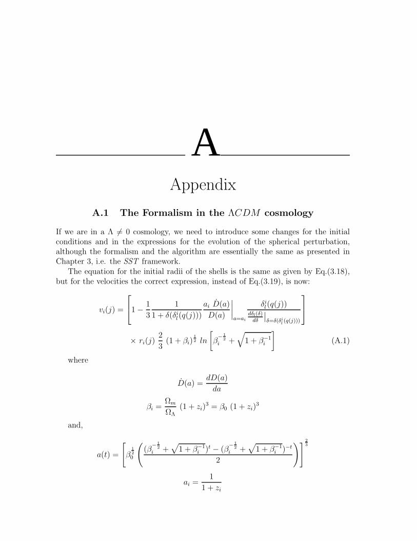
AAppendix
A.1 The Formalism in the ΛCDM cosmology
If we are in a Λ 6= 0 cosmology, we need to introduce some changes for the initialconditions and in the expressions for the evolution of the spherical perturbation,although the formalism and the algorithm are essentially the same as presented inChapter 3, i.e. the SST framework.
The equation for the initial radii of the shells is the same as given by Eq.(3.18),but for the velocities the correct expression, instead of Eq.(3.19), is now:
vi(j) =
1 − 1
3
1
1 + δ(δil(q(j)))
ai D(a)
D(a)
∣
∣
∣
∣
a=ai
δil(q(j))
dδl(δ)dδ
∣
∣
δ=δ(δil(q(j)))
× ri(j)2
3(1 + βi)
12 ln
[
β− 1
2i +
√
1 + β−1i
]
(A.1)
where
D(a) =dD(a)
da
βi =Ωm
ΩΛ(1 + zi)
3 = β0 (1 + zi)3
and,
a(t) =
[
β120
(
(β− 1
2i +
√
1 + β−1i )t − (β
− 12
i +√
1 + β−1i )−t
2
)]
23
ai =1
1 + zi
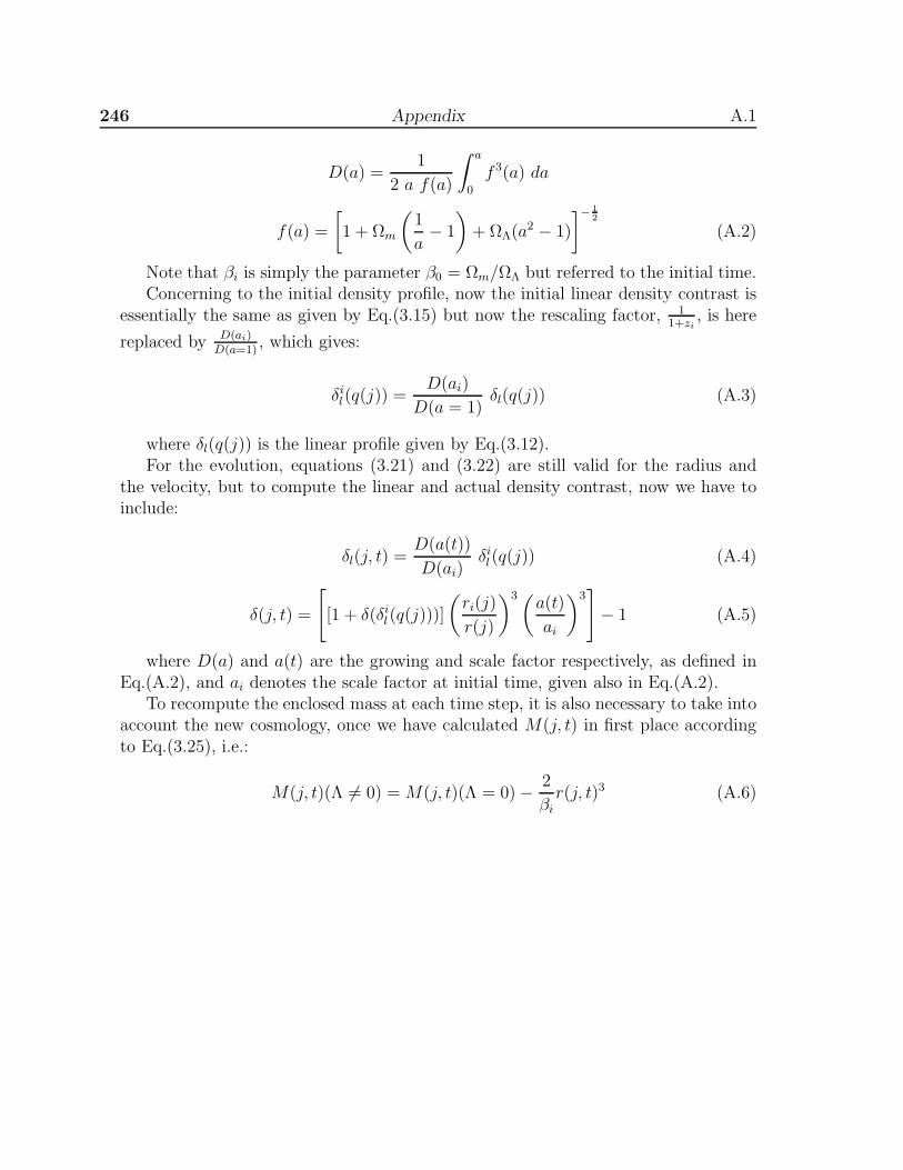
246 Appendix A.1
D(a) =1
2 a f(a)
∫ a
0
f 3(a) da
f(a) =
[
1 + Ωm
(
1
a− 1
)
+ ΩΛ(a2 − 1)
]− 12
(A.2)
Note that βi is simply the parameter β0 = Ωm/ΩΛ but referred to the initial time.Concerning to the initial density profile, now the initial linear density contrast is
essentially the same as given by Eq.(3.15) but now the rescaling factor, 11+zi
, is here
replaced by D(ai)D(a=1)
, which gives:
δil(q(j)) =
D(ai)
D(a = 1)δl(q(j)) (A.3)
where δl(q(j)) is the linear profile given by Eq.(3.12).For the evolution, equations (3.21) and (3.22) are still valid for the radius and
the velocity, but to compute the linear and actual density contrast, now we have toinclude:
δl(j, t) =D(a(t))
D(ai)δil(q(j)) (A.4)
δ(j, t) =
[
[1 + δ(δil(q(j)))]
(
ri(j)
r(j)
)3(a(t)
ai
)3]
− 1 (A.5)
where D(a) and a(t) are the growing and scale factor respectively, as defined inEq.(A.2), and ai denotes the scale factor at initial time, given also in Eq.(A.2).
To recompute the enclosed mass at each time step, it is also necessary to take intoaccount the new cosmology, once we have calculated M(j, t) in first place accordingto Eq.(3.25), i.e.:
M(j, t)(Λ 6= 0) = M(j, t)(Λ = 0) − 2
βir(j, t)3 (A.6)
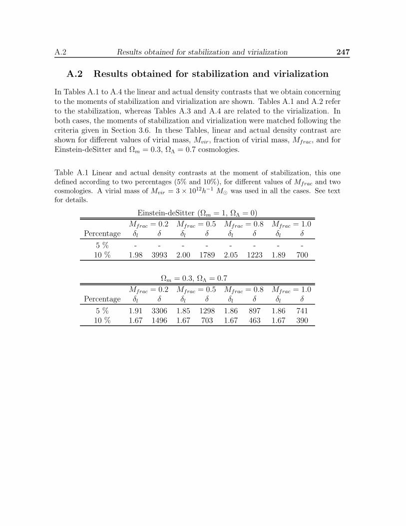
A.2 Results obtained for stabilization and virialization 247
A.2 Results obtained for stabilization and virialization
In Tables A.1 to A.4 the linear and actual density contrasts that we obtain concerningto the moments of stabilization and virialization are shown. Tables A.1 and A.2 referto the stabilization, whereas Tables A.3 and A.4 are related to the virialization. Inboth cases, the moments of stabilization and virialization were matched following thecriteria given in Section 3.6. In these Tables, linear and actual density contrast areshown for different values of virial mass, Mvir, fraction of virial mass, Mfrac, and forEinstein-deSitter and Ωm = 0.3, ΩΛ = 0.7 cosmologies.
Table A.1 Linear and actual density contrasts at the moment of stabilization, this onedefined according to two percentages (5% and 10%), for different values of Mfrac and twocosmologies. A virial mass of Mvir = 3 × 10¹²h−1 M⊙ was used in all the cases. See textfor details.
Einstein-deSitter (Ωm = 1, ΩΛ = 0)
Mfrac = 0.2 Mfrac = 0.5 Mfrac = 0.8 Mfrac = 1.0Percentage δl δ δl δ δl δ δl δ
5 % - - - - - - - -10 % 1.98 3993 2.00 1789 2.05 1223 1.89 700
Ωm = 0.3, ΩΛ = 0.7
Mfrac = 0.2 Mfrac = 0.5 Mfrac = 0.8 Mfrac = 1.0Percentage δl δ δl δ δl δ δl δ
5 % 1.91 3306 1.85 1298 1.86 897 1.86 74110 % 1.67 1496 1.67 703 1.67 463 1.67 390
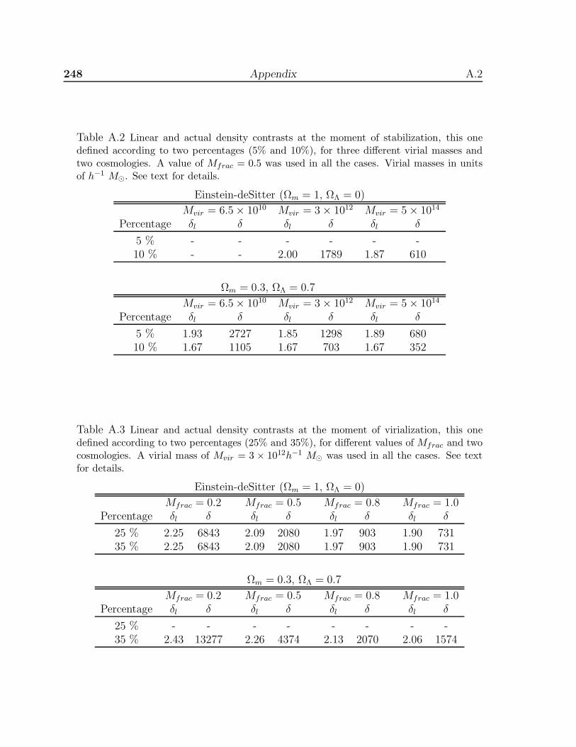
248 Appendix A.2
Table A.2 Linear and actual density contrasts at the moment of stabilization, this onedefined according to two percentages (5% and 10%), for three different virial masses andtwo cosmologies. A value of Mfrac = 0.5 was used in all the cases. Virial masses in unitsof h−1 M⊙. See text for details.
Einstein-deSitter (Ωm = 1, ΩΛ = 0)
Mvir = 6.5 × 10¹⁰ Mvir = 3 × 10¹² Mvir = 5 × 10¹⁴
Percentage δl δ δl δ δl δ
5 % - - - - - -10 % - - 2.00 1789 1.87 610
Ωm = 0.3, ΩΛ = 0.7
Mvir = 6.5 × 10¹⁰ Mvir = 3 × 10¹² Mvir = 5 × 10¹⁴
Percentage δl δ δl δ δl δ
5 % 1.93 2727 1.85 1298 1.89 68010 % 1.67 1105 1.67 703 1.67 352
Table A.3 Linear and actual density contrasts at the moment of virialization, this onedefined according to two percentages (25% and 35%), for different values of Mfrac and twocosmologies. A virial mass of Mvir = 3 × 10¹²h−1 M⊙ was used in all the cases. See textfor details.
Einstein-deSitter (Ωm = 1, ΩΛ = 0)
Mfrac = 0.2 Mfrac = 0.5 Mfrac = 0.8 Mfrac = 1.0Percentage δl δ δl δ δl δ δl δ
25 % 2.25 6843 2.09 2080 1.97 903 1.90 73135 % 2.25 6843 2.09 2080 1.97 903 1.90 731
Ωm = 0.3, ΩΛ = 0.7
Mfrac = 0.2 Mfrac = 0.5 Mfrac = 0.8 Mfrac = 1.0Percentage δl δ δl δ δl δ δl δ
25 % - - - - - - - -35 % 2.43 13277 2.26 4374 2.13 2070 2.06 1574
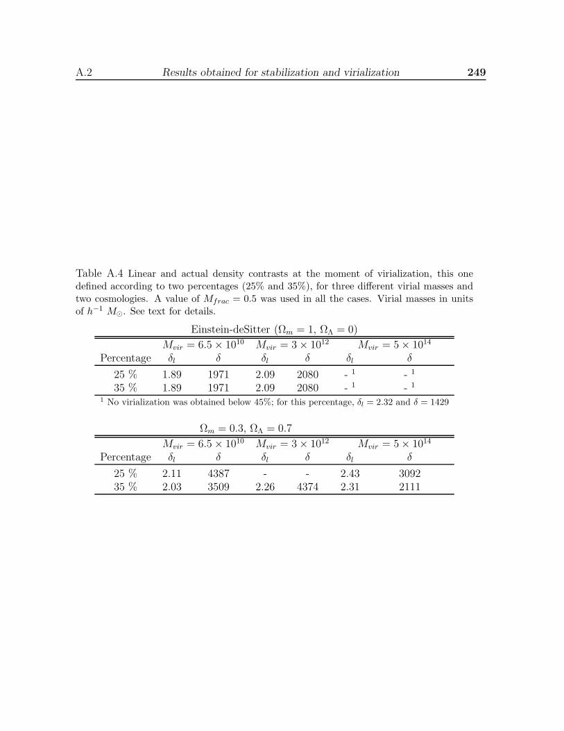
A.2 Results obtained for stabilization and virialization 249
Table A.4 Linear and actual density contrasts at the moment of virialization, this onedefined according to two percentages (25% and 35%), for three different virial masses andtwo cosmologies. A value of Mfrac = 0.5 was used in all the cases. Virial masses in unitsof h−1 M⊙. See text for details.
Einstein-deSitter (Ωm = 1, ΩΛ = 0)
Mvir = 6.5 × 10¹⁰ Mvir = 3 × 10¹² Mvir = 5 × 10¹⁴
Percentage δl δ δl δ δl δ
25 % 1.89 1971 2.09 2080 - 1 - 1
35 % 1.89 1971 2.09 2080 - 1 - 1
1 No virialization was obtained below 45%; for this percentage, δl = 2.32 and δ = 1429
Ωm = 0.3, ΩΛ = 0.7
Mvir = 6.5 × 10¹⁰ Mvir = 3 × 10¹² Mvir = 5 × 10¹⁴
Percentage δl δ δl δ δl δ
25 % 2.11 4387 - - 2.43 309235 % 2.03 3509 2.26 4374 2.31 2111

250 Appendix A.2

BPublications
Publications in refereed journals
19 refereed publications. A total of 323 citations in the ADS (7-Jul-09).
1. How far do they go? The outer structure of dark matter halosF. Prada, A.A. Klypin, E. Simonneau, J. Betancort-Rijo, S. G. Patiri, S.Gottlober and M. A. Sanchez-Conde, 2006, ApJ, 645, 1001
2. Detailed theoretical predictions of the outskirts of dark matter halosJ. E. Betancort-Rijo, M. A. Sanchez-Conde, F. Prada and S. G. Patiri, 2006,ApJ, 649, 579
3. The spherical collapse model with shell crossingM. A. Sanchez-Conde, J. Betancort-Rijo and F. Prada, 2007, MNRAS, 378,339
4. Dark Matter Annihilation in Draco: new considerations of the expected gammafluxM. A. Sanchez-Conde, F. Prada, E. W. Lokas, M. E. Gomez, R. Wojtak andM. Moles, 2007, Phys. Rev. D, 76, 123509
5. Upper limit for gamma-ray emission above 140 GeV from the dwarf spheroidalgalaxy DracoAlbert et al. (including M. A. Sanchez-Conde, 2008, ApJ, 679, 428
252 Publications B
6. The dark outside: the density profile of dark matter haloes beyond the virialradiusH. Tavıo, A. J. Cuesta, F. Prada, A. A. Klypin, M. A. Sanchez-Conde, 2008,MNRAS submitted, astro-ph/0807.3027
7. Upper limits on the VHE gamma-ray emission from the Willman 1 satellitegalaxy with the MAGIC telescopeAliu E. et al. (corresponding author M. A. Sanchez-Conde), 2009, ApJ, 697,1299
8. Hints of the existence of Axion-Like-Particles from the gamma-ray spectra ofcosmological sourcesM. A. Sanchez-Conde, D. Paneque, E. Bloom, F. Prada and A. Domınguez,2009, Phys. Rev. D, 79, 123511
11 more refereed publications as a member of the MAGIC collaboration:
1. Very-High-Energy gamma rays from a Distant Quasar: How Transparent Is theUniverse?Albert et al. (including M. A. Sanchez-Conde), 2008, Science, 320, 1752
2. Multiwavelength (Radio, X-Ray, and γ-Ray) Observations of the γ-Ray BinaryLS I +61 303Albert et al. (including M. A. Sanchez-Conde), 2008, ApJ, 684, 1351
3. Very High Energy Gamma-Ray Observations of Strong Flaring Activity in M87in 2008 FebruaryAlbert et al. (including M. A. Sanchez-Conde), 2008, ApJ, 685, L23
4. First Bounds on the High-Energy Emission from Isolated Wolf-Rayet BinarySystemsAliu et al. (including M. A. Sanchez-Conde), 2008, ApJ, 685, L71
5. Probing quantum gravity using photons from a flare of the active galactic nucleusMarkarian 501 observed by the MAGIC telescopeAlbert et al. (including M. A. Sanchez-Conde), 2008, Physics Letters B,668, 253
6. Observation of Pulsed γ-Rays Above 25 GeV From the Crab Pulsar with MAGICAliu et al. (including M. A. Sanchez-Conde), 2008, Science, 322, 1221
7. Improving the performance of the single-dish Cherenkov telescope MAGIC throughthe use of signal timingAliu et al. (including M. A. Sanchez-Conde), 2009, Astroparticle Physics,30, 293
B 253
8. The June 2008 Flare of Markarian 421 from Optical to TeV EnergiesDonnarumma et al. (including M. A. Sanchez-Conde), 2009, ApJL, 691, 13
9. Discovery of a very high energy gamma-ray signal from the 3C 66A/B regionAliu et al. (including M. A. Sanchez-Conde), 2008, ApJL, 692, 29
10. Periodic Very High Energy γ-Ray Emission from LS I +61 303 Observed withthe MAGIC TelescopeAlbert et al. (including M. A. Sanchez-Conde), 2009, ApJ, 693, 303
11. MAGIC upper limits to the VHE gamma-ray flux of 3C 454.3 in high emissionstateAnderhub et al. (including M. A. Sanchez-Conde), 2009, A&A, 498, 83
Publications in non-refereed journals
1. Dark Matter in Draco: new considerations of the expected gamma flux in IACTsSanchez-Conde M. A., Prada F., & Lokas E. L., 2006, The Dark Side of theUniverse, AIP Conference Proceedings, 878, 125
2. Characteristics and Performance of the GAW Experiment for a Large Field ofView Cerenkov Gamma-ray TelescopeCusumano, G., et al. (including M. A. Sanchez-Conde), 2006, Chinese Jour-nal of Astronomy and Astrophysics, Supplement, 6, S1, 369
3. Gamma Air Watch (GAW) - An Imaging Atmospheric Cherenkov TelescopeLarge with Large Field of ViewMineo T. et al. (including M. A. Sanchez-Conde), Proceedings of the ThirdWorkshop on Science with the New Generation of High Energy Gamma-rayExperiments, May 30 - June 1, 2005, Cividale del Friuli, Italy. World ScientificPublishing Co., Pte. Ltd., Singapore, 2006, p.75
4. Science with the new generation high energy gamma- ray experimentsAlvarez, M., et al. (including M. A. Sanchez-Conde), Proceedings of the 5thSCINEGHE Workshop, June 18-20, 2007; Frascati Physics Series vol.45, 2007,astro-ph/0712.1548
5. GAW - An Imaging Atmospheric Cherenkov Telescope with Large Field of ViewCusumano, G., et al. (including M. A. Sanchez-Conde), Proceedings of 30thICRC, International Cosmic Ray Conference 2007, Merida, Yucatan, Mexico,3-11 July 2007, astro-ph/0707.4541

254 Publications B
6. Indirect Dark Matter Search in Dwarf GalaxiesRissi M., et al. (including M. A. Sanchez-Conde), 2007, AstronomischeNachrichten, 328, 683
7. Dark Matter annihilation in Draco: new considerations of the expected gammafluxSanchez-Conde M. A., The First GLAST Symposium, AIP Conference Pro-ceedings, 2007, 921, 510
8. The search for DM in nearby dSph galaxies with MAGIC: candidates, resultsand prospectsSanchez-Conde M. A., to appear in the 8th UCLA Dark Matter ConferenceProceedings, Marina del Rey, CA, USA, February 2008
9. GAW - An Imaging Atmospheric Cherenkov Telescope with Large Field of ViewCusumano G. et al. (including M. A. Sanchez-Conde), 2008, InternationalCosmic Ray Conference, 3, 1317
10. Study of indirect detection of Axion-Like-Particles with the Fermi-LAT instru-ment and Imaging Atmospheric Cherenkov TelescopesPaneque, D., Bloom, E., & Sanchez-Conde, M. A., 2009, APS Meeting Ab-stracts, 12007
11. Search for Dark Matter signatures with MAGIC-I and prospects for MAGICPhase-IILombardi, S., et al., (including M. A. Sanchez-Conde), 2009, arXiv:0907.0738