The Gauss-Bonnet theorem for cone manifolds

and volumes of moduli spaces

Curtis McMullen

Schwarz, Picard, Deligne--Mostow, Cohen--Wolfart, Parker, Sauter,....

Kappes--Möller (2012) Thurston (1998)

Allendoerfer--Weil (1943)

10 Holomorphic Galois conjugation

Let V ! ! ! A2 be a Teichmuller curve on a Hilbert modular surface. Inthis final section we observe that V is covered by the graph of a remarkableholomorphic map F : H " H intertwining the action of a discrete groupG ! SL2(R) and its indiscrete Galois conjugate G!.

F

Figure 6. A holomorphic map from an ideal pentagon to an ideal star.

Curves on surfaces. Let f : V " M2 be a Teichmuller curve generatedby (X,!2). Assume that SL(X,!) has real quadratic trace field K ! R. Letk #" k! denote the Galois involution of K/Q, sending a + b

$d to a % b

$d,

and let g #" g! denote the corresponding involution on SL2(K).We have seen that Jac(Xt), t = f(t), admits real multiplication by K

for all t. Let ! = H/", " ! SL2(K), be the Hilbert modular surfaceparameterizing all Abelian varieties with the given action of K, as in §6.Then we obtain a commutative diagram

H %%%%" Vf%%%%" M2

!

!!"!!"

!!"

H2 %%%%" ! %%%%" A2

(10.1)

as in Corollary 7.3.If we make a change of basepoint for V , by replacing (X,!) with A·(X,!),

A & SL2(R), then f(V ) ! M2 does not change and GL(X,!) varies only byconjugation by A. The main observation of this section is:

Theorem 10.1 After a suitable change of basepoint, we have GL(X,!) !GL2(K) and "(t) = (t, F (t)), where F : H " H satisfies

F (g · t) = g! · F (t)

34

Illustration

Avg of |F′|2 in the hyperbolic metric?

Γ Γ′

-1+1/2+1/5 = -3/10 -1+1/2+2/5 = -1/10

Holomorphic Galois conjugationAnswer: 1/3

2

5

∞

5/2

2 ∞orbifold cone manifold

F

1-1

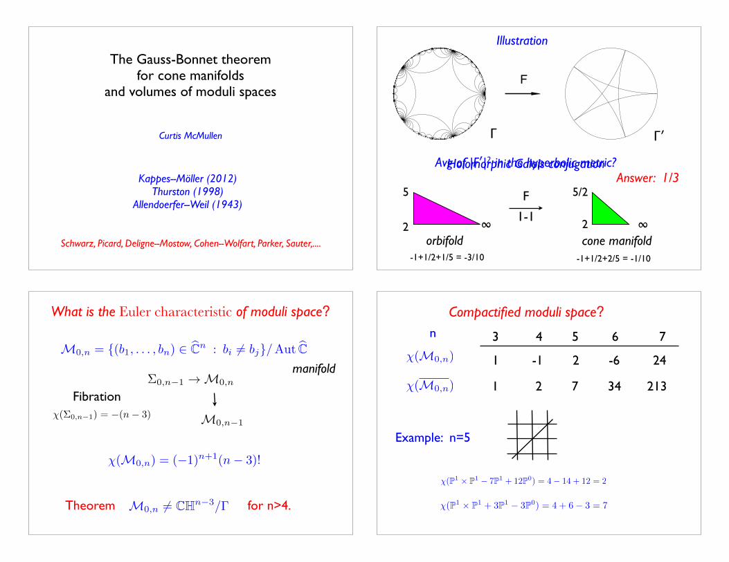
What is the Euler characteristic of moduli space?

M0,n = {(b1, . . . , bn) 2 bCn : bi 6= bj}/Aut bCmanifold

Fibration⌃0,n�1 ! M0,n

M0,n�1

�(M0,n) = (�1)n+1(n� 3)!

�(⌃0,n�1) = �(n� 3)

Theorem M0,n 6= CHn�3/� for n>4.

Compactified moduli space?

�(M0,n)

�(M0,n)

n 3 4 5 6 7

1 -1 2 -6 24

1 2 7 34 213

Example: n=5

�(P1 ⇥ P1 � 7P1 + 12P0) = 4� 14 + 12 = 2

�(P1 ⇥ P1 + 3P1 � 3P0) = 4 + 6� 3 = 7

Generating functions

Moduli spaces in genus zero and inversion

of power series

Curtis T. McMullen!

1 October 2012

Let M0,n denote the moduli space Riemann surfaces of genus 0 withn ordered marked points. Its Deligne-Mumford compactification M0,n isnaturally partitioned into connected strata of the form

S != M0,n1" · · ·"M0,ns

,

indexed by the di!erent topological types of stable curves with n markedpoints. The stable curves in the stratum above have s irreducible compo-nents and s# 1 nodes; thus

!

ni = n+ 2s# 2.This note provides a short proof of the following result, which shows the

universal formula for inversion of power series is encoded in the stratificationof moduli space.

Theorem 1 The formal inverse of f(x) = x #!

"

2 anxn/n! is given by

g(x) = x+!

"

2 bnxn/n!, where

bn ="

an1· · · ans

"

#

the number of strata S $ M0,n+1

isomorphic to M0,n1+1 " · · ·"M0,ns+1

$

·

That is, g(f(x)) = x.

Here the coe"cients of f(x) and g(x) are regarded as elements of the poly-nomial ring Q[a2, a3, . . .], and the sum is over all s % 1 and all multi-indices(n1, . . . , ns) with ni % 2.

Using basic properties of the Euler characteristic, we obtain:

Corollary 2 (Getzler) The generating functions

f(x) = x#""

n=2

!(M0,n+1)xn

n!and g(x) = x+

""

n=2

!(M0,n+1)xn

n!

are formal inverses of one another.

!Research supported in part by the NSF.

1Universal; via stable trees (M, L’Ens. math.)

Proof. The number of ribbon structures on a given stable rooted tree !is given by

!

(d(v) ! 1)!. The group Aut(!) acts freely on the space ofribbon structures, so ! contributes

!

(d(v) ! 1)!/|Aut(!)| identical termsto equation (1) for G(x). Similarly, ! contributes N(!)!/|Aut(!)| terms toequation (2) for g(x). Setting An = an/n!, we find F (x) = f(x) and

G(x) ="

marked !

!

(d(v) ! 1)!

N(!)!A(!)xN(!) = g(x),

so f(g(x)) = F (G(x)) = x.

Remark. The same reasoning shows (2) can be rewritten as

f!1(x) ="

stable !

N(!) + 1

|Aut(!)|a(!)xN(!).

For example, using the trees shown in Figure 2 we find

f!1(x) = x+a22x2 +

(a3 + 3a22)

6x3 +

(a4 + 10a2a3 + 15a32)

24x4 +O(x5).

For a quite di!erent approach to Corollary 4, see [Ge2, Thm 1.3].

Figure 2. The stable trees with N(!) " 4.

Proof of Theorem 1. A stable curveX # M0,n+1 of genus zero determinesmarked tree t(X) whose interior vertices correspond to the irreducible com-ponents of X, and whose edges correspond to its nodes and labeled points.Conversely, any marked tree with N(!) $ 2 can be realized by a stablecurve, so the map

! %& S(!) = {X # M0,N(!)+1 : t(X) '= !}

gives a bijection between marked trees with N(!) $ 2 and the strata ofmoduli spaces. The desired inversion formula now follows from the precedingCorollary.

4

Proof. The number of ribbon structures on a given stable rooted tree !is given by

!

(d(v) ! 1)!. The group Aut(!) acts freely on the space ofribbon structures, so ! contributes

!

(d(v) ! 1)!/|Aut(!)| identical termsto equation (1) for G(x). Similarly, ! contributes N(!)!/|Aut(!)| terms toequation (2) for g(x). Setting An = an/n!, we find F (x) = f(x) and

G(x) ="

marked !

!

(d(v) ! 1)!

N(!)!A(!)xN(!) = g(x),

so f(g(x)) = F (G(x)) = x.

Remark. The same reasoning shows (2) can be rewritten as

f!1(x) ="

stable !

N(!) + 1

|Aut(!)|a(!)xN(!).

For example, using the trees shown in Figure 2 we find

f!1(x) = x+a22x2 +

(a3 + 3a22)

6x3 +

(a4 + 10a2a3 + 15a32)

24x4 +O(x5).

For a quite di!erent approach to Corollary 4, see [Ge2, Thm 1.3].

Figure 2. The stable trees with N(!) " 4.

Proof of Theorem 1. A stable curveX # M0,n+1 of genus zero determinesmarked tree t(X) whose interior vertices correspond to the irreducible com-ponents of X, and whose edges correspond to its nodes and labeled points.Conversely, any marked tree with N(!) $ 2 can be realized by a stablecurve, so the map

! %& S(!) = {X # M0,N(!)+1 : t(X) '= !}

gives a bijection between marked trees with N(!) $ 2 and the strata ofmoduli spaces. The desired inversion formula now follows from the precedingCorollary.

4

n=4 n=5

Moduli spaces of polyhedra...

Fix µ1, . . . , µn, 0 < µi < 1,P

µi = 2.

! =dxQn

1 (x� bi)µi(!) =

Xµibi

divisor of degree 2

Any (bi) determines a meromorphic 1-form on

bC:

(

bC, |!|) ⇠=

convex polyhedron in R3

Cone angles 2⇡(1� µi).

Example: n=12, μi = 1/6

... are complex hyperbolic after all

= moduli space of cone metrics on S2 with given angles

M0,n(µ)

Schwarz, Picard, Deligne-Mostow, Thurston, 1986 Math Olympiad

Theorem: M0,n(µ) is naturally a complex hyperbolic manifold

(locally CHn�3, via periods of !)

Example: μ = (7,7,7,7,8)/18

7 7

77

8

X : y18 = (x� b1) · · · (x� b4)

M0,5 ! Mg, g = 25

7/18 q = ⇣�718

Signature (1,2)

(bi) 7! (positive line in C1,2)

⇠=

CH2

[!] = [dx/y7] 2 H1(X)q

Z/18 acts on H1(X)

Also get rep of braid group B4 → U(1,2)

(Burau)

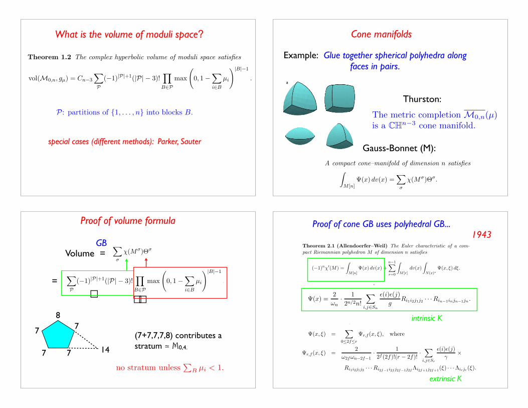
What is the volume of moduli space?

invariant under the holonomy of K; while K itself can be assembled fromspherical simplices by gluing their faces together in pairs.

A cone manifold is naturally partitioned into connected strata M!, eachof which is a totally geodesic Riemannian manifold. The solid angle of Mat x, defined by

!(x) = limr!0

voln(B(x, r))

voln(Bn)rn,

is a constant along each stratum; its value on M! will be denoted by !!.Let M [n] denote the union of top–dimensional strata of M . In §7 we

will show:

Theorem 1.1 A compact cone–manifold of dimension n satisfies!

M [n]"(x) dv(x) =

"

!

!(M!)!!.

For a smooth manifold the right-hand side reduces to !(M) and weobtain the usual Gauss–Bonnet formula. For orbifolds the right-hand termshave rational weights of the form !! = 1/|H! |, and we obtain Satake’sformula [Sat]. In a cone manifold !! can assume any positive real value,and the right-hand side provides a natural generalization of the orbifoldEuler characteristic of M .

Moduli spaces. Let M0,n denote the moduli space of configurations ofn ! 3 ordered points on the Riemann sphere. Generalizing work of Pi-card and Deligne–Mostow, Thurston showed that for any set of real weights(µ1, . . . , µn) with 0 < µi < 1 and

#µi = 2, we have a natural complex

hyperbolic metric gµ on M0,n, and its metric completion P (µ) is a cone–manifold [Th].

Applying Theorem 1.1, in §8 we will show:

Theorem 1.2 The complex hyperbolic volume of moduli space satisfies

vol(M0,n, gµ) = Cn"3

"

P

("1)|P|+1(|P| " 3)!$

B#P

max

%

0, 1""

i#B

µi

&|B|"1

.

Here P ranges over all partitions of {1, . . . , n} into blocks B, and Ck =("4")k/(k + 1)! is the value of "(x) on a complex hyperbolic k-manifold.Previously the volume has been computed only in special cases [Yo], [Sau],[Par].

Orbifolds and volume ratios. There are 94 values of µ with n ! 5such that a natural finite quotient M(µ) of P (µ) is a complex hyperbolic

2

P: partitions of {1, . . . , n} into blocks B.

special cases (different methods): Parker, Sauter

Cone manifolds

Example: Glue together spherical polyhedra along faces in pairs.

Thurston:

The metric completion M0,n(µ)is a CHn�3

cone manifold.

invariant under the holonomy of K; while K itself can be assembled fromspherical simplices by gluing their faces together in pairs.

A cone manifold is naturally partitioned into connected strata M!, eachof which is a totally geodesic Riemannian manifold. The solid angle of Mat x, defined by

!(x) = limr!0

voln(B(x, r))

voln(Bn)rn,

is a constant along each stratum; its value on M! will be denoted by !!.Let M [n] denote the union of top–dimensional strata of M . In §7 we

will show:

Theorem 1.1 A compact cone–manifold of dimension n satisfies!

M [n]"(x) dv(x) =

"

!

!(M!)!!.

For a smooth manifold the right-hand side reduces to !(M) and weobtain the usual Gauss–Bonnet formula. For orbifolds the right-hand termshave rational weights of the form !! = 1/|H! |, and we obtain Satake’sformula [Sat]. In a cone manifold !! can assume any positive real value,and the right-hand side provides a natural generalization of the orbifoldEuler characteristic of M .

Moduli spaces. Let M0,n denote the moduli space of configurations ofn ! 3 ordered points on the Riemann sphere. Generalizing work of Pi-card and Deligne–Mostow, Thurston showed that for any set of real weights(µ1, . . . , µn) with 0 < µi < 1 and

#µi = 2, we have a natural complex

hyperbolic metric gµ on M0,n, and its metric completion P (µ) is a cone–manifold [Th].

Applying Theorem 1.1, in §8 we will show:

Theorem 1.2 The complex hyperbolic volume of moduli space satisfies

vol(M0,n, gµ) = Cn"3

"

P

("1)|P|+1(|P| " 3)!$

B#P

max

%

0, 1""

i#B

µi

&|B|"1

.

Here P ranges over all partitions of {1, . . . , n} into blocks B, and Ck =("4")k/(k + 1)! is the value of "(x) on a complex hyperbolic k-manifold.Previously the volume has been computed only in special cases [Yo], [Sau],[Par].

Orbifolds and volume ratios. There are 94 values of µ with n ! 5such that a natural finite quotient M(µ) of P (µ) is a complex hyperbolic

2

Gauss-Bonnet (M):

Proof of volume formula

87

77

7

14

invariant under the holonomy of K; while K itself can be assembled fromspherical simplices by gluing their faces together in pairs.

A cone manifold is naturally partitioned into connected strata M!, eachof which is a totally geodesic Riemannian manifold. The solid angle of Mat x, defined by

!(x) = limr!0

voln(B(x, r))

voln(Bn)rn,

is a constant along each stratum; its value on M! will be denoted by !!.Let M [n] denote the union of top–dimensional strata of M . In §7 we

will show:

Theorem 1.1 A compact cone–manifold of dimension n satisfies!

M [n]"(x) dv(x) =

"

!

!(M!)!!.

For a smooth manifold the right-hand side reduces to !(M) and weobtain the usual Gauss–Bonnet formula. For orbifolds the right-hand termshave rational weights of the form !! = 1/|H! |, and we obtain Satake’sformula [Sat]. In a cone manifold !! can assume any positive real value,and the right-hand side provides a natural generalization of the orbifoldEuler characteristic of M .

Moduli spaces. Let M0,n denote the moduli space of configurations ofn ! 3 ordered points on the Riemann sphere. Generalizing work of Pi-card and Deligne–Mostow, Thurston showed that for any set of real weights(µ1, . . . , µn) with 0 < µi < 1 and

#µi = 2, we have a natural complex

hyperbolic metric gµ on M0,n, and its metric completion P (µ) is a cone–manifold [Th].

Applying Theorem 1.1, in §8 we will show:

Theorem 1.2 The complex hyperbolic volume of moduli space satisfies

vol(M0,n, gµ) = Cn"3

"

P

("1)|P|+1(|P| " 3)!$

B#P

max

%

0, 1""

i#B

µi

&|B|"1

.

Here P ranges over all partitions of {1, . . . , n} into blocks B, and Ck =("4")k/(k + 1)! is the value of "(x) on a complex hyperbolic k-manifold.Previously the volume has been computed only in special cases [Yo], [Sau],[Par].

Orbifolds and volume ratios. There are 94 values of µ with n ! 5such that a natural finite quotient M(µ) of P (µ) is a complex hyperbolic

2

invariant under the holonomy of K; while K itself can be assembled fromspherical simplices by gluing their faces together in pairs.

A cone manifold is naturally partitioned into connected strata M!, eachof which is a totally geodesic Riemannian manifold. The solid angle of Mat x, defined by

!(x) = limr!0

voln(B(x, r))

voln(Bn)rn,

is a constant along each stratum; its value on M! will be denoted by !!.Let M [n] denote the union of top–dimensional strata of M . In §7 we

will show:

Theorem 1.1 A compact cone–manifold of dimension n satisfies!

M [n]"(x) dv(x) =

"

!

!(M!)!!.

For a smooth manifold the right-hand side reduces to !(M) and weobtain the usual Gauss–Bonnet formula. For orbifolds the right-hand termshave rational weights of the form !! = 1/|H! |, and we obtain Satake’sformula [Sat]. In a cone manifold !! can assume any positive real value,and the right-hand side provides a natural generalization of the orbifoldEuler characteristic of M .

Moduli spaces. Let M0,n denote the moduli space of configurations ofn ! 3 ordered points on the Riemann sphere. Generalizing work of Pi-card and Deligne–Mostow, Thurston showed that for any set of real weights(µ1, . . . , µn) with 0 < µi < 1 and

#µi = 2, we have a natural complex

hyperbolic metric gµ on M0,n, and its metric completion P (µ) is a cone–manifold [Th].

Applying Theorem 1.1, in §8 we will show:

Theorem 1.2 The complex hyperbolic volume of moduli space satisfies

vol(M0,n, gµ) = Cn"3

"

P

("1)|P|+1(|P| " 3)!$

B#P

max

%

0, 1""

i#B

µi

&|B|"1

.

Here P ranges over all partitions of {1, . . . , n} into blocks B, and Ck =("4")k/(k + 1)! is the value of "(x) on a complex hyperbolic k-manifold.Previously the volume has been computed only in special cases [Yo], [Sau],[Par].

Orbifolds and volume ratios. There are 94 values of µ with n ! 5such that a natural finite quotient M(µ) of P (µ) is a complex hyperbolic

2

Volume = GB

= � ��

(7+7,7,7,8) contributes a stratum ≃ M0,4.

no stratum unless

PB µi < 1.

along a codimension two submanifold; see e.g. [Cg], [HMM], [FST], [Ko1],[Br], [Tr] and [AB]. A general account of the theory of stratified spaces isgiven in [Pf].

The first proof of the Gauss–Bonnet theorem for general manifolds wasgiven by Allendoerfer and Weil [AW], using Weyl’s tube formula [We].Chern’s intrinsic proof [Cn] appeared shortly thereafter. The tube formulaand its applications in di!erential geometry are treated in [Gr]. Theorem1.1 can be extended to cone manifolds with curved strata by using the fullstrength of the formula for polyhedra.

The volume of M0,n with respect to its natural symplectic structure iscomputed in [Zo]. The Euler characteristic of the Deligne-Mumford com-pactification M0,n can be computed using inversion of powers series; see[Ge], [Mc3]. The compactifications M(µ) resulting from a choice of weightsare usual di!erent from M0,n, and depend on µ; they are discussed fromthe perspective of algebraic geometry in [Ha].

Acknowledgements. I would like to thank Kappes and Moller for usefulcorrespondence.

2 Polyhedra

The Gauss–Bonnet formula for polyhedra may be stated as follows.

Theorem 2.1 (Allendoerfer–Weil) The Euler characteristic of a com-pact Riemannian polyhedron M of dimension n satisfies

(!1)n!!(M) =

!

M [n]"(x) dv(x) +

n"1"

r=0

!

M [r]dv(x)

!

N(x)!"(x, ") d".

Here !!(M) = !(M)! !(#M).In this section we explain the formula above and the basic properties of

its integrand.

Spheres and duality. Let Sn denote the unit sphere in Rn+1, and letBn+1 denote the unit ball. We let

$n = 2 · (4%)n/2(n/2)!

n!,

denote the volume of Sn, with the convention that (n/2)! = #(n2 +1) if n isodd.

4

A convex spherical polyhedron is a set K ! Sn obtained by intersectingfinitely many hemispheres. Its dual is given by

K! = {x " Sn : #x, y$ % 0 &y " K}.

When the ambient sphere needs to emphasized, we will writeK! = (K,Sn)!.

Manifolds. Let A be a smooth Riemannian manifold of dimension n. Whenn is even, the intrinsic Gauss–Bonnet integrand on A is given in terms ofthe Riemann curvature tensor by

!(x) =2

!n· 1

2n/2n!

!

i,j"Sn

"(i)"(j)

gRi1i2j1j2 · · ·Rin!1injn!1jn .

Here "(i) and "(j) denote the signs of the permutations i and j, and g isthe determinant of the metric. When n is odd, we set !(x) = 0. TheGauss–Bonnet theorem states that for any closed manifold A we have

#(A) =

"

A!(x) dv(x).

Submanifolds. Now let A be an r-dimensional submanifold of a Rieman-nian manifold B of dimension n. Let Rijkl denote the restriction of theRiemann curvature tensor on B to A, and let "ij($) denote the second fun-damental form — a symmetric tensor on A depending linearly on a normalvector $. In local coordinates where A ! B is modeled on Rr ! Rn, we have

"ij($) = #'eiej , $$.

The extrinsic Gauss–Bonnet integrand is the function on the unit normalbundle to A defined by

!(x, $) =!

0#2f#r

!r,f(x, $), where

!r,f (x, $) =2

!2f!n$2f$1· 1

2f (2f)!(r ( 2f)!·!

i,j"Sr

"(i)"(j)

%)

Ri1i2j1j2 · · ·Ri2f!1i2f j2f!1j2f"i2f+1j2f+1($) · · ·"irjr($).

Here % is the determinant of the induced metric on A.The intrinsic and extrinsic integrands on A are related by

!(x) =

"

S(x)!(x, $) d$, (2.1)

5

A convex spherical polyhedron is a set K ! Sn obtained by intersectingfinitely many hemispheres. Its dual is given by

K! = {x " Sn : #x, y$ % 0 &y " K}.

When the ambient sphere needs to emphasized, we will writeK! = (K,Sn)!.

Manifolds. Let A be a smooth Riemannian manifold of dimension n. Whenn is even, the intrinsic Gauss–Bonnet integrand on A is given in terms ofthe Riemann curvature tensor by

!(x) =2

!n· 1

2n/2n!

!

i,j"Sn

"(i)"(j)

gRi1i2j1j2 · · ·Rin!1injn!1jn .

Here "(i) and "(j) denote the signs of the permutations i and j, and g isthe determinant of the metric. When n is odd, we set !(x) = 0. TheGauss–Bonnet theorem states that for any closed manifold A we have

#(A) =

"

A!(x) dv(x).

Submanifolds. Now let A be an r-dimensional submanifold of a Rieman-nian manifold B of dimension n. Let Rijkl denote the restriction of theRiemann curvature tensor on B to A, and let "ij($) denote the second fun-damental form — a symmetric tensor on A depending linearly on a normalvector $. In local coordinates where A ! B is modeled on Rr ! Rn, we have

"ij($) = #'eiej , $$.

The extrinsic Gauss–Bonnet integrand is the function on the unit normalbundle to A defined by

!(x, $) =!

0#2f#r

!r,f(x, $), where

!r,f (x, $) =2

!2f!n$2f$1· 1

2f (2f)!(r ( 2f)!·!

i,j"Sr

"(i)"(j)

%)

Ri1i2j1j2 · · ·Ri2f!1i2f j2f!1j2f"i2f+1j2f+1($) · · ·"irjr($).

Here % is the determinant of the induced metric on A.The intrinsic and extrinsic integrands on A are related by

!(x) =

"

S(x)!(x, $) d$, (2.1)

5

Proof of cone GB uses polyhedral GB...1943

extrinsic K

intrinsic K

When M is endowed with a smooth metric, it becomes a Riemannianpolyhedron [AW].

Given an n-dimensional Riemannian polyhedron and r < n, we let M [r]denote the union of the r-dimensional faces of !M , and let M [n] = M!!M .Each face of M can be regarded as a submanifold of a slight thickening ofM [n], so its normal bundle and its extrinsic Gauss–Bonnet integrand aredefined. Given x " M [r], r < n, we let N(x) # S(x) denote the convex setof unit vectors normal to M [r] that point into M [n].

Sketch of the proof of Gauss–Bonnet. These definitions complete thestatement of the Gauss–Bonnet formula for polyhedra (Theorem 2.1). Weconclude with a sketch of the proof; for details, see [AW, Theorem II].

First suppose M is a simplex. Choose an isometric embedding M "$RN+1 for some large N . Let T # RN+1 be the boundary of a small tubearound the image, i.e. the set of points at distance # > 0 from M . Let$ : T $ SN denote the Gauss map. For # su!ciently small, we also have anearest-point projection % : T $ M .

M[n]

T[r]M[r]

Figure 1. The tube around a polyhedron in RN+1.

Let T [r] = %!1(M [r]) be the subset of T closest to M [r]. Then for anyt " T [r] we have a vector & = $(t) " SN and a point x = %(t) " M [r]. Thepair (x, &) satisfies %&, v& = 0 for all v " TxM [r], and

%&, v& ' 0 (v " N(x) # TxRN+1.

Conversely, if (x, &) satisfies the conditions above, then there is unique t " Twith %(t) = x and $(t) = v. Using this fact and Weyl’s tube formula [We],one finds that the contributions to the degree of the Gauss map are givenby

G(M [n]) =1

'N

!

T [n]$"(d&) =

!

M [n]"(x) dv(x)

7

...which in turns comes from Weyl’s tube formula.

1939

Example: μ = (7,7,7,7,8)/18

7 7

77

8

7/18 q = ⇣�718

Signature (1,2)

(continued)

Galois 5 5

55

16

5/18

Signature (1,2)

q = ⇣�518

Non-arithmetic lattices (DM)

87

77

7

14

(18-14)/36 = 1/9

165

55

5

10

(18-10)/36 = 2/9

(� discrete) ⇠= (�0 dense) in U(1, 2).

Γ is a nonarithmetic lattice

orbifold

M0,n(µ)

⇠= CH2/�

M0,n

M0,n(µ0)

cone manifoldholonomy �

0

Invariants

Kappes-Möller

The volume ratios ⇢(µ, µ0) =

vol(M0,n(µ0))

vol(M0,n(µ))

are the same for all subgroups of finite index in Γ.

The 16 nonarithmetic lattices arisingfrom moduli spaces

fall into 9 commensurability classes.

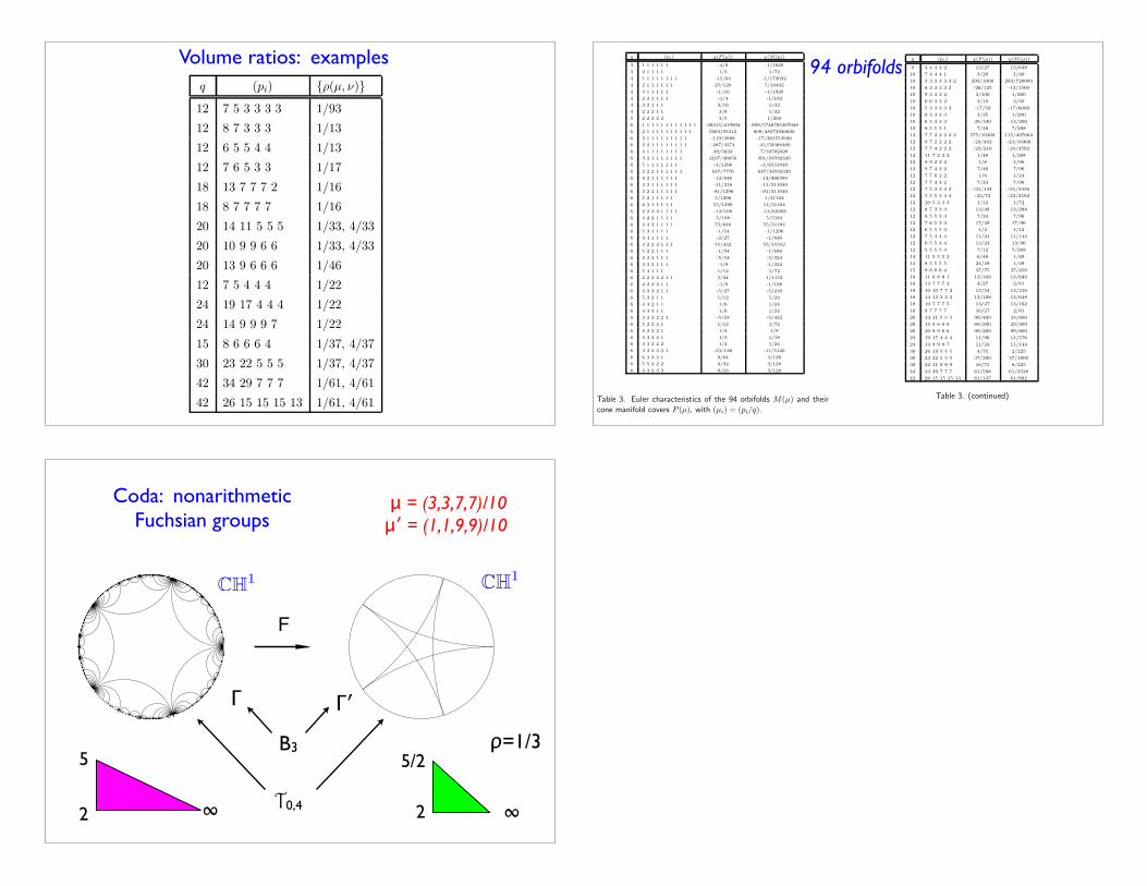
q (pi) {!(µ, ")}

12 7 5 3 3 3 3 1/93

12 8 7 3 3 3 1/13

12 6 5 5 4 4 1/13

12 7 6 5 3 3 1/17

18 13 7 7 7 2 1/16

18 8 7 7 7 7 1/16

20 14 11 5 5 5 1/33, 4/33

20 10 9 9 6 6 1/33, 4/33

20 13 9 6 6 6 1/46

12 7 5 4 4 4 1/22

24 19 17 4 4 4 1/22

24 14 9 9 9 7 1/22

15 8 6 6 6 4 1/37, 4/37

30 23 22 5 5 5 1/37, 4/37

42 34 29 7 7 7 1/61, 4/61

42 26 15 15 15 13 1/61, 4/61

Table 4. Nonarithmetic groups !(µ), with (µi) = (pi/q). These 16groups fall into 9 commensurability classes, which are distinguishedby the volume ratios given in the right column.

29

Volume ratios: examples q (pi) !(P (µ)) !(M(µ))

3 1 1 1 1 1 1 -4/9 -1/1620

3 2 1 1 1 1 1/3 1/72

4 1 1 1 1 1 1 1 1 -15/64 -1/172032

4 2 1 1 1 1 1 1 25/128 5/18432

4 3 1 1 1 1 1 -1/16 -1/1920

4 2 2 1 1 1 1 -1/4 -1/192

4 3 2 1 1 1 3/16 1/32

4 2 2 2 1 1 3/8 1/32

5 2 2 2 2 2 3/5 1/200

6 1 1 1 1 1 1 1 1 1 1 1 1 -28315/419904 -809/5746705367040

6 2 1 1 1 1 1 1 1 1 1 1 5663/93312 809/48372940800

6 3 1 1 1 1 1 1 1 1 1 -119/3888 -17/201553920

6 2 2 1 1 1 1 1 1 1 1 -287/4374 -41/50388480

6 4 1 1 1 1 1 1 1 1 49/5832 7/33592320

6 3 2 1 1 1 1 1 1 1 2107/46656 301/33592320

6 5 1 1 1 1 1 1 1 -1/1296 -1/6531840

6 2 2 2 1 1 1 1 1 1 637/7776 637/33592320

6 4 2 1 1 1 1 1 1 -13/648 -13/466560

6 3 3 1 1 1 1 1 1 -11/216 -11/311040

6 3 2 2 1 1 1 1 1 -91/1296 -91/311040

6 5 2 1 1 1 1 1 5/1296 1/31104

6 4 3 1 1 1 1 1 55/1296 11/31104

6 2 2 2 2 1 1 1 1 -13/108 -13/62208

6 4 2 2 1 1 1 1 5/108 5/5184

6 3 3 2 1 1 1 1 55/648 55/31104

6 5 3 1 1 1 1 -1/54 -1/1296

6 4 4 1 1 1 1 -2/27 -1/648

6 3 2 2 2 1 1 1 55/432 55/15552

6 5 2 2 1 1 1 -1/54 -1/648

6 4 3 2 1 1 1 -5/54 -5/324

6 3 3 3 1 1 1 -1/9 -1/324

6 5 4 1 1 1 1/12 1/72

6 2 2 2 2 2 1 1 5/24 1/1152

6 4 2 2 2 1 1 -1/9 -1/108

6 3 3 2 2 1 1 -5/27 -5/216

6 5 3 2 1 1 1/12 1/24

6 4 4 2 1 1 1/6 1/24

6 4 3 3 1 1 1/6 1/24

6 3 2 2 2 2 1 -5/18 -5/432

6 5 2 2 2 1 1/12 1/72

6 4 3 2 2 1 1/4 1/8

6 3 3 3 2 1 1/3 1/18

6 3 3 2 2 2 1/2 1/24

8 3 3 3 3 3 1 -33/128 -11/5120

8 6 3 3 3 1 9/64 3/128

8 5 5 2 2 2 9/32 3/128

8 4 3 3 3 3 9/16 3/128

Table 3. Euler characteristics of the 94 orbifolds M(µ) and theircone manifold covers P (µ), with (µi) = (pi/q).

25

q (pi) !(P (µ)) !(M(µ))

9 4 4 4 4 2 13/27 13/648

10 7 4 4 4 1 3/20 1/40

10 3 3 3 3 3 3 2 293/1000 293/720000

10 6 3 3 3 3 2 -26/125 -13/1500

10 9 3 3 3 2 3/100 1/200

10 6 6 3 3 2 3/10 3/40

10 5 3 3 3 3 3 -17/50 -17/6000

10 8 3 3 3 3 3/25 1/200

10 6 5 3 3 3 39/100 13/200

12 8 5 5 5 1 7/48 7/288

12 7 7 2 2 2 2 2 575/10368 115/497664

12 9 7 2 2 2 2 -23/432 -23/10368

12 7 7 4 2 2 2 -23/216 -23/2592

12 11 7 2 2 2 1/48 1/288

12 9 9 2 2 2 1/8 1/96

12 9 7 4 2 2 7/48 7/96

12 7 7 6 2 2 1/6 1/24

12 7 7 4 4 2 7/24 7/96

12 7 5 3 3 3 3 -31/144 -31/3456

12 5 5 5 3 3 3 -23/72 -23/2592

12 10 5 3 3 3 1/12 1/72

12 8 7 3 3 3 13/48 13/288

12 8 5 5 3 3 7/24 7/96

12 7 6 5 3 3 17/48 17/96

12 6 5 5 5 3 1/2 1/12

12 7 5 4 4 4 11/24 11/144

12 6 5 5 4 4 13/24 13/96

12 5 5 5 5 4 7/12 7/288

14 11 5 5 5 2 6/49 1/49

14 8 5 5 5 5 24/49 1/49

15 8 6 6 6 4 37/75 37/450

18 11 8 8 8 1 13/108 13/648

18 13 7 7 7 2 4/27 2/81

18 10 10 7 7 2 13/54 13/216

18 14 13 3 3 3 13/108 13/648

18 10 7 7 7 5 13/27 13/162

18 8 7 7 7 7 16/27 2/81

20 14 11 5 5 5 99/400 33/800

20 13 9 6 6 6 69/200 23/400

20 10 9 9 6 6 99/200 99/800

24 19 17 4 4 4 11/96 11/576

24 14 9 9 9 7 11/24 11/144

30 26 19 5 5 5 4/75 2/225

30 23 22 5 5 5 37/300 37/1800

30 22 11 9 9 9 16/75 8/225

42 34 29 7 7 7 61/588 61/3528

42 26 15 15 15 13 61/147 61/882

Table 3. (continued)

26

94 orbifolds

μ = (3,3,7,7)/10μ′ = (1,1,9,9)/10

10 Holomorphic Galois conjugation

Let V ! ! ! A2 be a Teichmuller curve on a Hilbert modular surface. Inthis final section we observe that V is covered by the graph of a remarkableholomorphic map F : H " H intertwining the action of a discrete groupG ! SL2(R) and its indiscrete Galois conjugate G!.

F

Figure 6. A holomorphic map from an ideal pentagon to an ideal star.

Curves on surfaces. Let f : V " M2 be a Teichmuller curve generatedby (X,!2). Assume that SL(X,!) has real quadratic trace field K ! R. Letk #" k! denote the Galois involution of K/Q, sending a + b

$d to a % b

$d,

and let g #" g! denote the corresponding involution on SL2(K).We have seen that Jac(Xt), t = f(t), admits real multiplication by K

for all t. Let ! = H/", " ! SL2(K), be the Hilbert modular surfaceparameterizing all Abelian varieties with the given action of K, as in §6.Then we obtain a commutative diagram

H %%%%" Vf%%%%" M2

!

!!"!!"

!!"

H2 %%%%" ! %%%%" A2

(10.1)

as in Corollary 7.3.If we make a change of basepoint for V , by replacing (X,!) with A·(X,!),

A & SL2(R), then f(V ) ! M2 does not change and GL(X,!) varies only byconjugation by A. The main observation of this section is:

Theorem 10.1 After a suitable change of basepoint, we have GL(X,!) !GL2(K) and "(t) = (t, F (t)), where F : H " H satisfies

F (g · t) = g! · F (t)

34

Γ Γ′B3

T0,4

CH1 CH1

2

5

∞

5/2

2 ∞

Coda: nonarithmetic Fuchsian groups

ρ=1/3