![EXPANDER GRAPHS, PROPERTY AND APPROXIMATE GROUPS · (D). Random walks on groups, the spectral radius and Kesten’s criterion. In his 1959 Cornell thesis [76], Kesten studied random](https://static.fdocument.org/doc/165x107/5f1ee70b1d41ee5aa62b2c20/expander-graphs-property-and-approximate-d-random-walks-on-groups-the-spectral.jpg)
The Einstein relation for random walks on Galton …The Einstein relation for random walks on...
47
The Einstein relation for random walks on Galton–Watson trees Ofer Zeitouni Weizmann Institute and University of Minnesota Joint with G. Ben Arous, Y. Hu, S. Olla June 2011 Ofer Zeitouni Stat Phys Day June 2011 1 / 12
Transcript of The Einstein relation for random walks on Galton …The Einstein relation for random walks on...
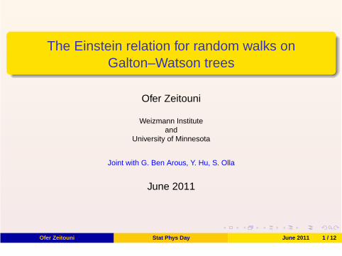
The Einstein relation for random walks onGalton–Watson trees
Ofer Zeitouni
Weizmann Instituteand
University of Minnesota
Joint with G. Ben Arous, Y. Hu, S. Olla
June 2011
Ofer Zeitouni Stat Phys Day June 2011 1 / 12

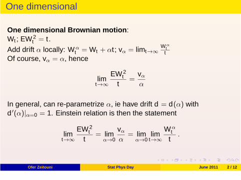
One dimensional
One dimensional Brownian motion:Wt ; EW 2
t = t .
Add drift α locally: Wαt = Wt + αt ; vα = limt→∞
Wαtt
Of course, vα = α, hence
limt→∞
EW 2t
t=
vαα
In general, can re-parametrize α, ie have drift d = d(α) withd ′(α)|α=0 = 1. Einstein relation is then the statement
limt→∞
EW 2t
t= lim
α→0
vαα
= limα→0
limt→∞
Wαt
t.
Ofer Zeitouni Stat Phys Day June 2011 2 / 12
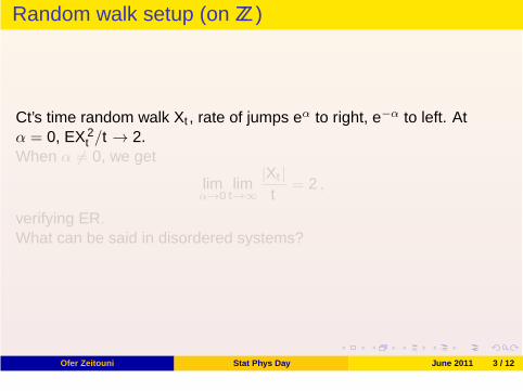
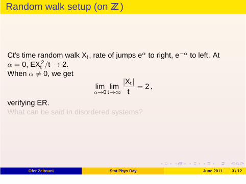
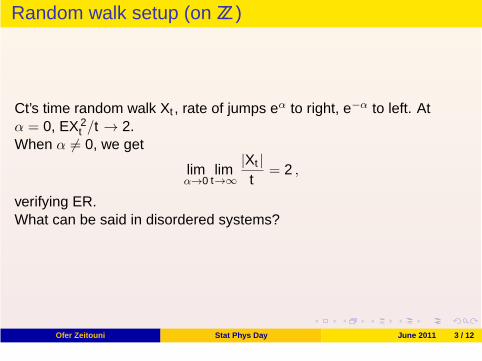
Random walk setup (on ZZ )
Ct’s time random walk Xt , rate of jumps eα to right, e−α to left. Atα = 0, EX 2
t /t → 2.When α 6= 0, we get
limα→0
limt→∞
|Xt |t
= 2 ,
verifying ER.What can be said in disordered systems?
Ofer Zeitouni Stat Phys Day June 2011 3 / 12
Random walk setup (on ZZ )
Ct’s time random walk Xt , rate of jumps eα to right, e−α to left. Atα = 0, EX 2
t /t → 2.When α 6= 0, we get
limα→0
limt→∞
|Xt |t
= 2 ,
verifying ER.What can be said in disordered systems?
Ofer Zeitouni Stat Phys Day June 2011 3 / 12
Random walk setup (on ZZ )
Ct’s time random walk Xt , rate of jumps eα to right, e−α to left. Atα = 0, EX 2
t /t → 2.When α 6= 0, we get
limα→0
limt→∞
|Xt |t
= 2 ,
verifying ER.What can be said in disordered systems?
Ofer Zeitouni Stat Phys Day June 2011 3 / 12
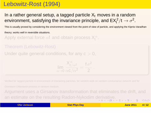
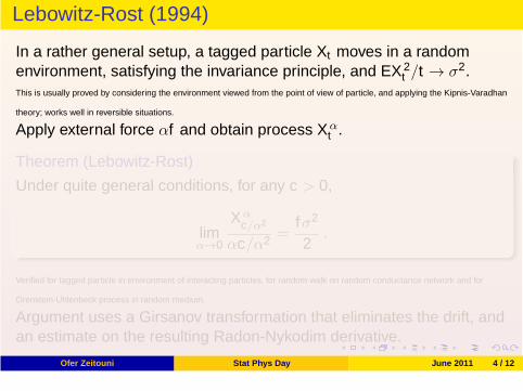
Lebowitz-Rost (1994)
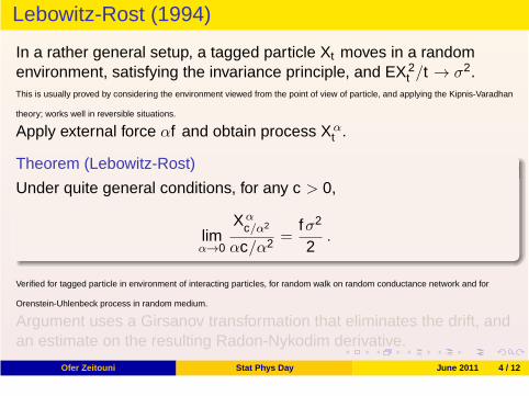
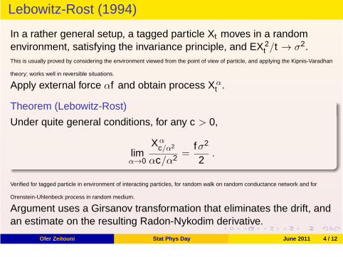
In a rather general setup, a tagged particle Xt moves in a randomenvironment, satisfying the invariance principle, and EX 2
t /t → σ2.This is usually proved by considering the environment viewed from the point of view of particle, and applying the Kipnis-Varadhan
theory; works well in reversible situations.
Apply external force αf and obtain process Xαt .
Theorem (Lebowitz-Rost)
Under quite general conditions, for any c > 0,
limα→0
Xαc/α2
αc/α2 =fσ2
2.
Verified for tagged particle in environment of interacting particles, for random walk on random conductance network and for
Orenstein-Uhlenbeck process in random medium.
Argument uses a Girsanov transformation that eliminates the drift, andan estimate on the resulting Radon-Nykodim derivative.
Ofer Zeitouni Stat Phys Day June 2011 4 / 12
Lebowitz-Rost (1994)
In a rather general setup, a tagged particle Xt moves in a randomenvironment, satisfying the invariance principle, and EX 2
t /t → σ2.This is usually proved by considering the environment viewed from the point of view of particle, and applying the Kipnis-Varadhan
theory; works well in reversible situations.
Apply external force αf and obtain process Xαt .
Theorem (Lebowitz-Rost)
Under quite general conditions, for any c > 0,
limα→0
Xαc/α2
αc/α2 =fσ2
2.
Verified for tagged particle in environment of interacting particles, for random walk on random conductance network and for
Orenstein-Uhlenbeck process in random medium.
Argument uses a Girsanov transformation that eliminates the drift, andan estimate on the resulting Radon-Nykodim derivative.
Ofer Zeitouni Stat Phys Day June 2011 4 / 12
Verification of ER
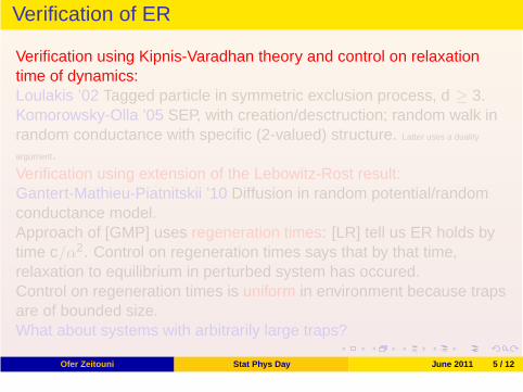
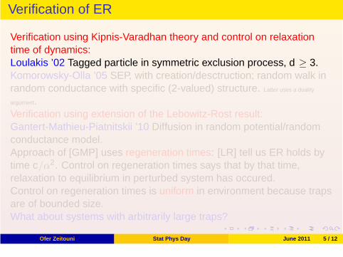
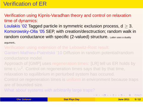
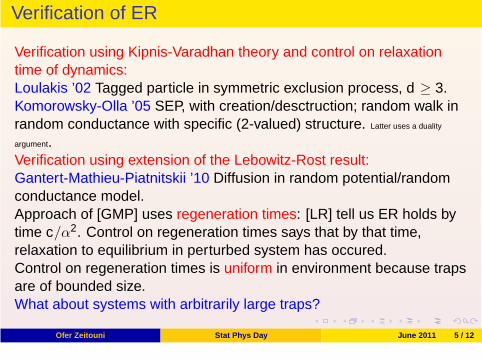
Verification using Kipnis-Varadhan theory and control on relaxationtime of dynamics:Loulakis ’02 Tagged particle in symmetric exclusion process, d ≥ 3.Komorowsky-Olla ’05 SEP, with creation/desctruction; random walk inrandom conductance with specific (2-valued) structure. Latter uses a duality
argument.Verification using extension of the Lebowitz-Rost result:Gantert-Mathieu-Piatnitskii ’10 Diffusion in random potential/randomconductance model.Approach of [GMP] uses regeneration times: [LR] tell us ER holds bytime c/α2. Control on regeneration times says that by that time,relaxation to equilibrium in perturbed system has occured.Control on regeneration times is uniform in environment because trapsare of bounded size.What about systems with arbitrarily large traps?
Ofer Zeitouni Stat Phys Day June 2011 5 / 12
Verification of ER
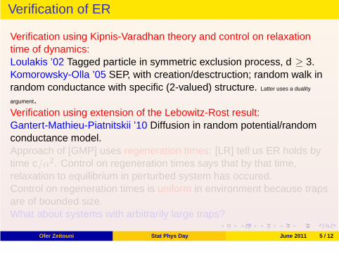
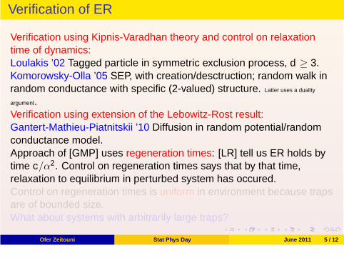
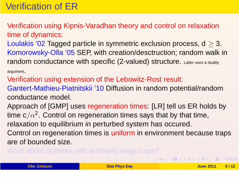
Verification using Kipnis-Varadhan theory and control on relaxationtime of dynamics:Loulakis ’02 Tagged particle in symmetric exclusion process, d ≥ 3.Komorowsky-Olla ’05 SEP, with creation/desctruction; random walk inrandom conductance with specific (2-valued) structure. Latter uses a duality
argument.Verification using extension of the Lebowitz-Rost result:Gantert-Mathieu-Piatnitskii ’10 Diffusion in random potential/randomconductance model.Approach of [GMP] uses regeneration times: [LR] tell us ER holds bytime c/α2. Control on regeneration times says that by that time,relaxation to equilibrium in perturbed system has occured.Control on regeneration times is uniform in environment because trapsare of bounded size.What about systems with arbitrarily large traps?
Ofer Zeitouni Stat Phys Day June 2011 5 / 12
Galton-Watson trees
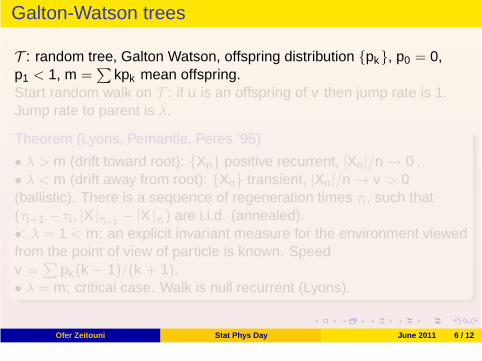
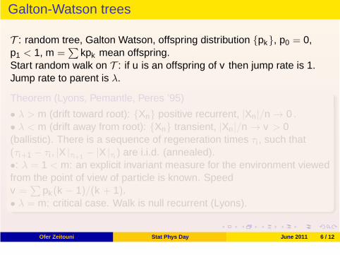
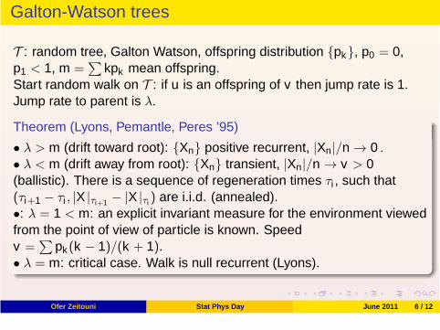
T : random tree, Galton Watson, offspring distribution {pk}, p0 = 0,p1 < 1, m =
∑
kpk mean offspring.Start random walk on T : if u is an offspring of v then jump rate is 1.Jump rate to parent is λ.
Theorem (Lyons, Pemantle, Peres ’95)
• λ > m (drift toward root): {Xn} positive recurrent, |Xn|/n → 0 .• λ < m (drift away from root): {Xn} transient, |Xn|/n → v > 0(ballistic). There is a sequence of regeneration times τi , such that(τi+1 − τi , |X |τi+1 − |X |τi ) are i.i.d. (annealed).•: λ = 1 < m: an explicit invariant measure for the environment viewedfrom the point of view of particle is known. Speedv =
∑
pk (k − 1)/(k + 1).• λ = m: critical case. Walk is null recurrent (Lyons).
Ofer Zeitouni Stat Phys Day June 2011 6 / 12
Galton-Watson trees
T : random tree, Galton Watson, offspring distribution {pk}, p0 = 0,p1 < 1, m =
∑
kpk mean offspring.Start random walk on T : if u is an offspring of v then jump rate is 1.Jump rate to parent is λ.
Theorem (Lyons, Pemantle, Peres ’95)
• λ > m (drift toward root): {Xn} positive recurrent, |Xn|/n → 0 .• λ < m (drift away from root): {Xn} transient, |Xn|/n → v > 0(ballistic). There is a sequence of regeneration times τi , such that(τi+1 − τi , |X |τi+1 − |X |τi ) are i.i.d. (annealed).•: λ = 1 < m: an explicit invariant measure for the environment viewedfrom the point of view of particle is known. Speedv =
∑
pk (k − 1)/(k + 1).• λ = m: critical case. Walk is null recurrent (Lyons).
Ofer Zeitouni Stat Phys Day June 2011 6 / 12
Galton-Watson trees - CLT
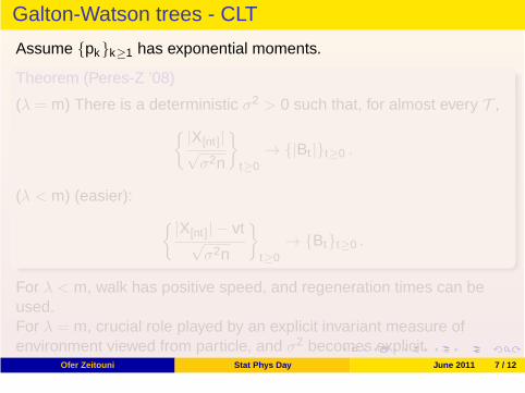
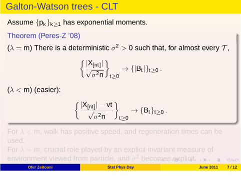
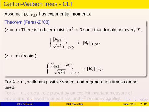
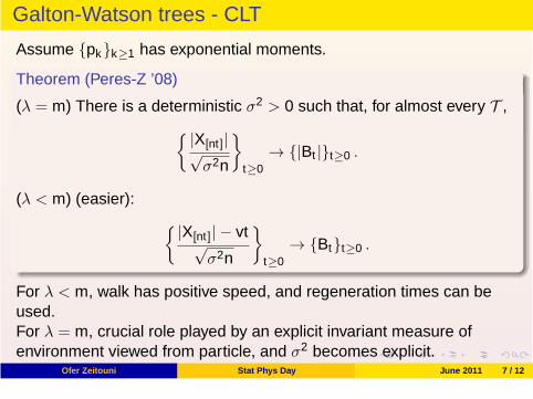
Assume {pk}k≥1 has exponential moments.
Theorem (Peres-Z ’08)
(λ = m) There is a deterministic σ2 > 0 such that, for almost every T ,{ |X[nt]|√
σ2n
}
t≥0→ {|Bt |}t≥0 .
(λ < m) (easier):{ |X[nt]| − vt√
σ2n
}
t≥0→ {Bt}t≥0 .
For λ < m, walk has positive speed, and regeneration times can beused.For λ = m, crucial role played by an explicit invariant measure ofenvironment viewed from particle, and σ2 becomes explicit.
Ofer Zeitouni Stat Phys Day June 2011 7 / 12
Galton-Watson trees - CLT
Assume {pk}k≥1 has exponential moments.
Theorem (Peres-Z ’08)
(λ = m) There is a deterministic σ2 > 0 such that, for almost every T ,{ |X[nt]|√
σ2n
}
t≥0→ {|Bt |}t≥0 .
(λ < m) (easier):{ |X[nt]| − vt√
σ2n
}
t≥0→ {Bt}t≥0 .
For λ < m, walk has positive speed, and regeneration times can beused.For λ = m, crucial role played by an explicit invariant measure ofenvironment viewed from particle, and σ2 becomes explicit.
Ofer Zeitouni Stat Phys Day June 2011 7 / 12
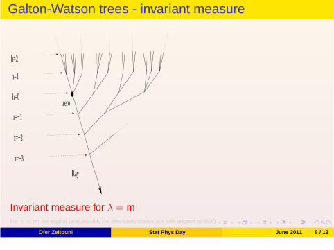
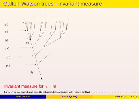
Galton-Watson trees - invariant measure
zero
Ray
h=−1
h=−2
h=−3
h=2
h=1
h=0
Invariant measure for λ = mFor λ < m: not explicit (and possibly not absolutely continuous with respect to IGW)
Ofer Zeitouni Stat Phys Day June 2011 8 / 12
Galton-Watson trees - invariant measure
zero
Ray
h=−1
h=−2
h=−3
h=2
h=1
h=0
Invariant measure for λ = mFor λ < m: not explicit (and possibly not absolutely continuous with respect to IGW)
Ofer Zeitouni Stat Phys Day June 2011 8 / 12
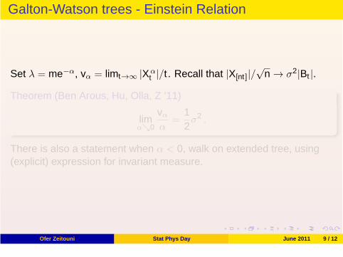
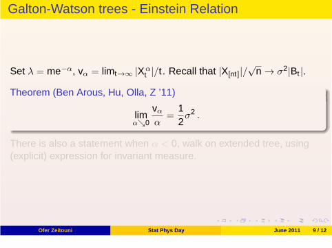
Galton-Watson trees - Einstein Relation
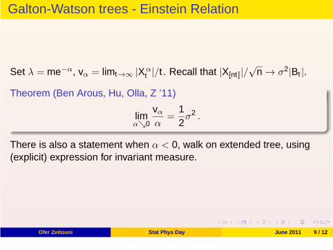
Set λ = me−α, vα = limt→∞ |Xαt |/t . Recall that |X[nt]|/
√n → σ2|Bt |.
Theorem (Ben Arous, Hu, Olla, Z ’11)
limαց0
vαα
=12σ2 .
There is also a statement when α < 0, walk on extended tree, using(explicit) expression for invariant measure.
Ofer Zeitouni Stat Phys Day June 2011 9 / 12
Galton-Watson trees - Einstein Relation
Set λ = me−α, vα = limt→∞ |Xαt |/t . Recall that |X[nt]|/
√n → σ2|Bt |.
Theorem (Ben Arous, Hu, Olla, Z ’11)
limαց0
vαα
=12σ2 .
There is also a statement when α < 0, walk on extended tree, using(explicit) expression for invariant measure.
Ofer Zeitouni Stat Phys Day June 2011 9 / 12
Galton-Watson trees - Proof of Einstein Relation
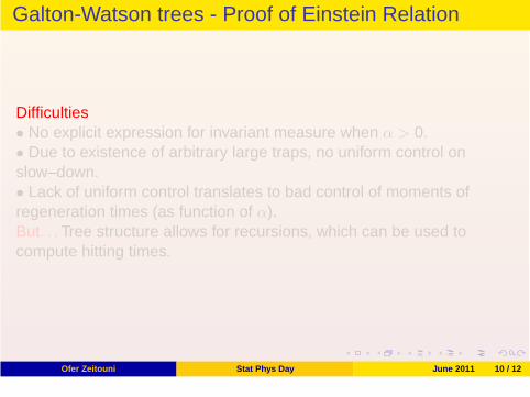
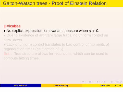
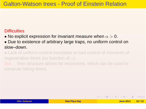
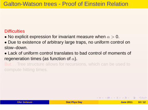
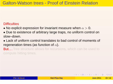
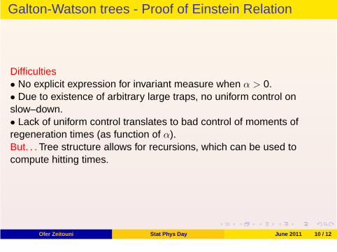
Difficulties• No explicit expression for invariant measure when α > 0.• Due to existence of arbitrary large traps, no uniform control onslow–down.• Lack of uniform control translates to bad control of moments ofregeneration times (as function of α).But. . . Tree structure allows for recursions, which can be used tocompute hitting times.
Ofer Zeitouni Stat Phys Day June 2011 10 / 12
Galton-Watson trees - Proof of Einstein Relation
Difficulties• No explicit expression for invariant measure when α > 0.• Due to existence of arbitrary large traps, no uniform control onslow–down.• Lack of uniform control translates to bad control of moments ofregeneration times (as function of α).But. . . Tree structure allows for recursions, which can be used tocompute hitting times.
Ofer Zeitouni Stat Phys Day June 2011 10 / 12
Some elements of proof of ER - basic recursion
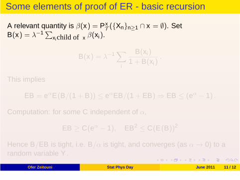
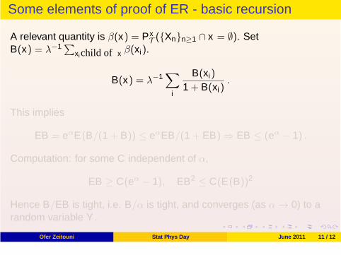
A relevant quantity is β(x) = PxT ({Xn}n≥1 ∩ x = ∅). Set
B(x) = λ−1 ∑
xichild of x β(xi).
B(x) = λ−1∑
i
B(xi)
1 + B(xi).
This implies
EB = eαE(B/(1 + B)) ≤ eαEB/(1 + EB) ⇒ EB ≤ (eα − 1) .
Computation: for some C independent of α,
EB ≥ C(eα − 1), EB2 ≤ C(E(B))2
Hence B/EB is tight, i.e. B/α is tight, and converges (as α → 0) to arandom variable Y .
Ofer Zeitouni Stat Phys Day June 2011 11 / 12
Some elements of proof of ER - basic recursion
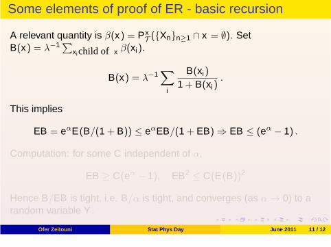
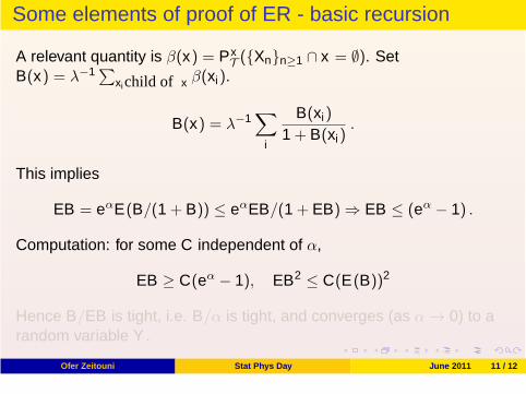
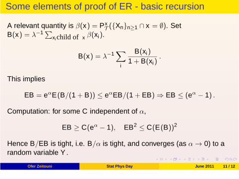
A relevant quantity is β(x) = PxT ({Xn}n≥1 ∩ x = ∅). Set
B(x) = λ−1 ∑
xichild of x β(xi).
B(x) = λ−1∑
i
B(xi)
1 + B(xi).
This implies
EB = eαE(B/(1 + B)) ≤ eαEB/(1 + EB) ⇒ EB ≤ (eα − 1) .
Computation: for some C independent of α,
EB ≥ C(eα − 1), EB2 ≤ C(E(B))2
Hence B/EB is tight, i.e. B/α is tight, and converges (as α → 0) to arandom variable Y .
Ofer Zeitouni Stat Phys Day June 2011 11 / 12
Some elements of proof of ER - basic recursion II
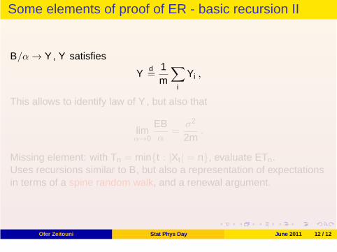
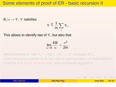
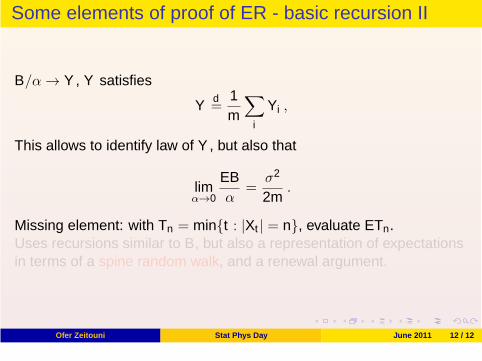
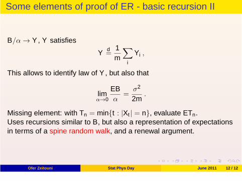
B/α → Y , Y satisfies
Y d=
1m
∑
i
Yi ,
This allows to identify law of Y , but also that
limα→0
EBα
=σ2
2m.
Missing element: with Tn = min{t : |Xt | = n}, evaluate ETn.Uses recursions similar to B, but also a representation of expectationsin terms of a spine random walk, and a renewal argument.
Ofer Zeitouni Stat Phys Day June 2011 12 / 12
Some elements of proof of ER - basic recursion II
B/α → Y , Y satisfies
Y d=
1m
∑
i
Yi ,
This allows to identify law of Y , but also that
limα→0
EBα
=σ2
2m.
Missing element: with Tn = min{t : |Xt | = n}, evaluate ETn.Uses recursions similar to B, but also a representation of expectationsin terms of a spine random walk, and a renewal argument.
Ofer Zeitouni Stat Phys Day June 2011 12 / 12