Discrete and continuous

quantum walks

Yevgeniy Kovchegov

Oregon State University

(based on joint work with R.Burton,

Z.Dimcovic and T.Nguyen)

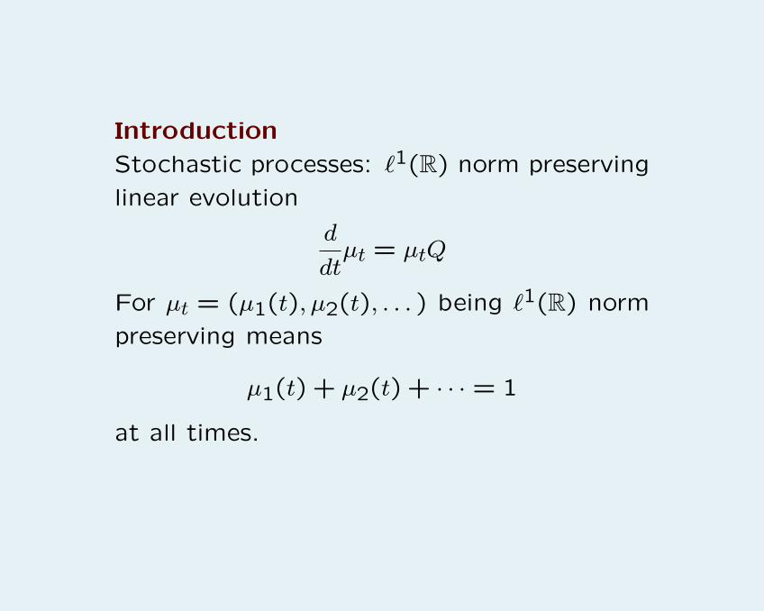
Introduction

Stochastic processes: `1(R) norm preserving

linear evolution

d

dtµt = µtQ

For µt = (µ1(t), µ2(t), . . . ) being `1(R) norm

preserving means

µ1(t) + µ2(t) + · · · = 1

at all times.

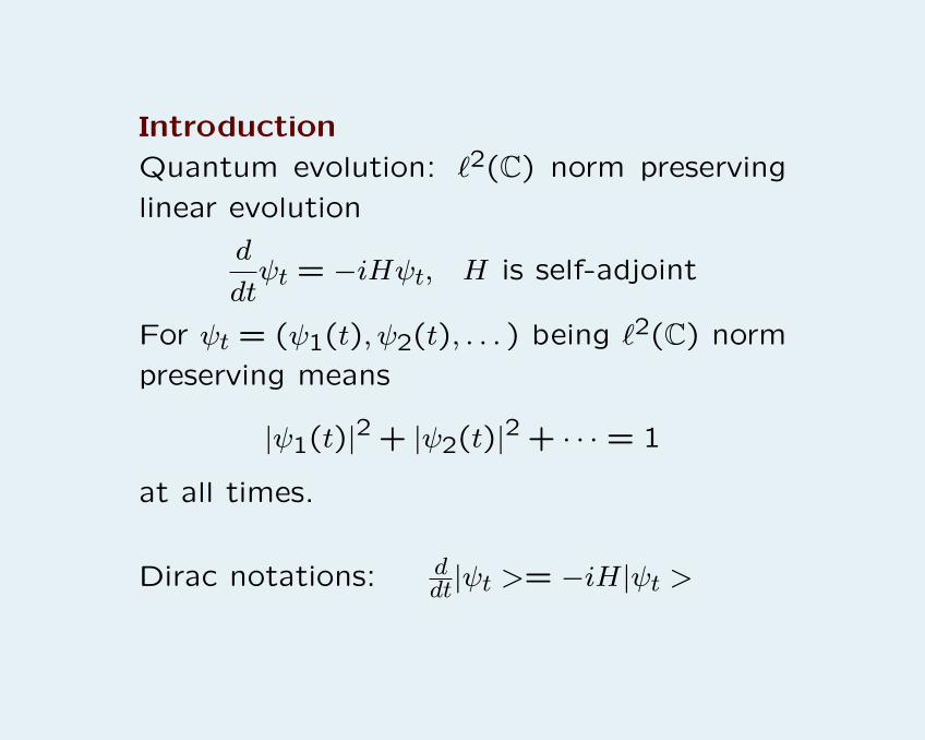
Introduction

Quantum evolution: `2(C) norm preserving

linear evolution

d

dtψt = −iHψt, H is self-adjoint

For ψt = (ψ1(t), ψ2(t), . . . ) being `2(C) norm

preserving means

|ψ1(t)|2 + |ψ2(t)|2 + · · · = 1

at all times.

Dirac notations: ddt|ψt >= −iH|ψt >

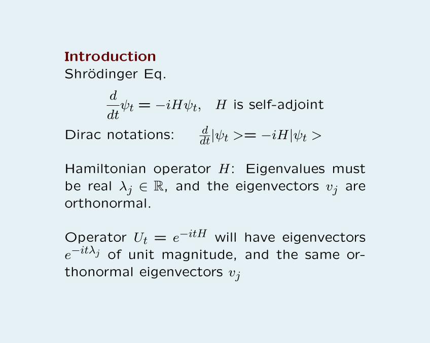
IntroductionShrodinger Eq.

d

dtψt = −iHψt, H is self-adjoint

Dirac notations: ddt|ψt >= −iH|ψt >

Hamiltonian operator H: Eigenvalues mustbe real λj ∈ R, and the eigenvectors vj areorthonormal.

Operator Ut = e−itH will have eigenvectorse−itλj of unit magnitude, and the same or-thonormal eigenvectors vj

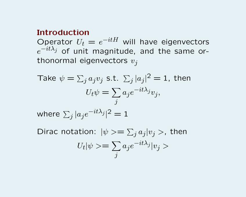
IntroductionOperator Ut = e−itH will have eigenvectorse−itλj of unit magnitude, and the same or-thonormal eigenvectors vj

Take ψ =∑j ajvj s.t.

∑j |aj|2 = 1, then

Utψ =∑j

aje−itλjvj,

where∑j |aje−itλj |2 = 1

Dirac notation: |ψ >=∑j aj|vj >, then

Ut|ψ >=∑j

aje−itλj |vj >

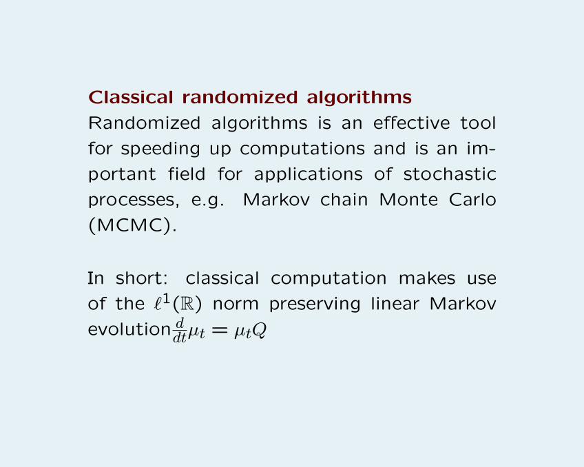
Classical randomized algorithms

Randomized algorithms is an effective tool

for speeding up computations and is an im-

portant field for applications of stochastic

processes, e.g. Markov chain Monte Carlo

(MCMC).

In short: classical computation makes use

of the `1(R) norm preserving linear Markov

evolution ddtµt = µtQ

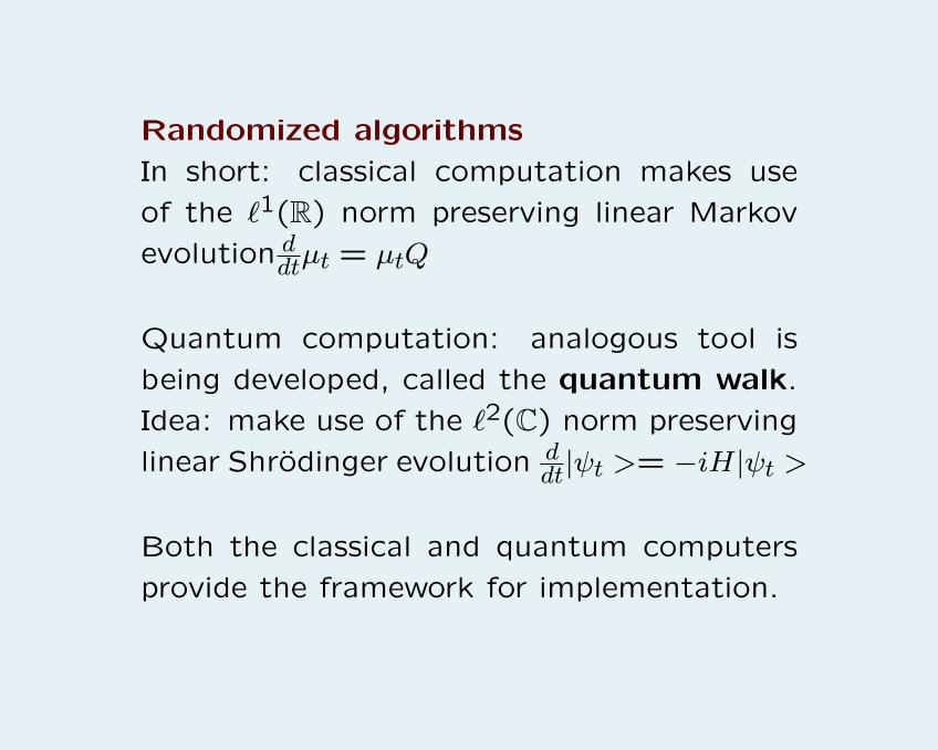
Randomized algorithms

In short: classical computation makes use

of the `1(R) norm preserving linear Markov

evolution ddtµt = µtQ

Quantum computation: analogous tool is

being developed, called the quantum walk.

Idea: make use of the `2(C) norm preserving

linear Shrodinger evolution ddt|ψt >= −iH|ψt >

Both the classical and quantum computers

provide the framework for implementation.

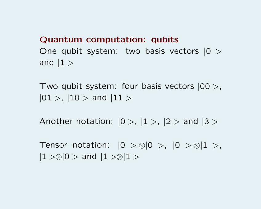
Quantum computation: qubits

One qubit system: two basis vectors |0 >

and |1 >

Two qubit system: four basis vectors |00 >,

|01 >, |10 > and |11 >

Another notation: |0 >, |1 >, |2 > and |3 >

Tensor notation: |0 >⊗|0 >, |0 >⊗|1 >,

|1 >⊗|0 > and |1 >⊗|1 >

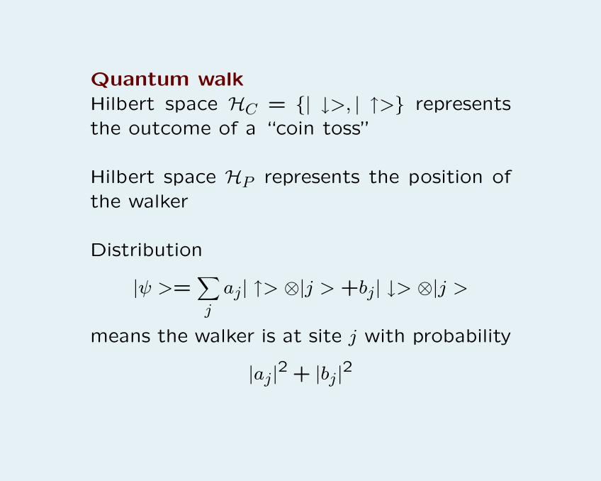
Quantum walkHilbert space HC = {| ↓>, | ↑>} representsthe outcome of a “coin toss”

Hilbert space HP represents the position ofthe walker

Distribution

|ψ >=∑j

aj| ↑> ⊗|j > +bj| ↓> ⊗|j >

means the walker is at site j with probability

|aj|2 + |bj|2

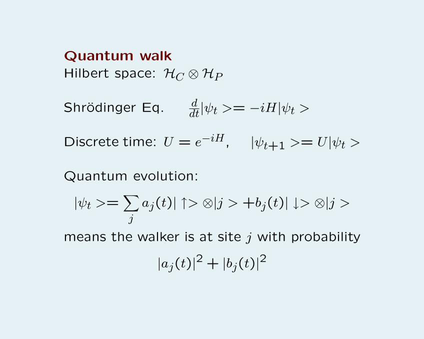
Quantum walkHilbert space: HC ⊗HP

Shrodinger Eq. ddt|ψt >= −iH|ψt >

Discrete time: U = e−iH, |ψt+1 >= U |ψt >

Quantum evolution:

|ψt >=∑j

aj(t)| ↑> ⊗|j > +bj(t)| ↓> ⊗|j >

means the walker is at site j with probability

|aj(t)|2 + |bj(t)|2

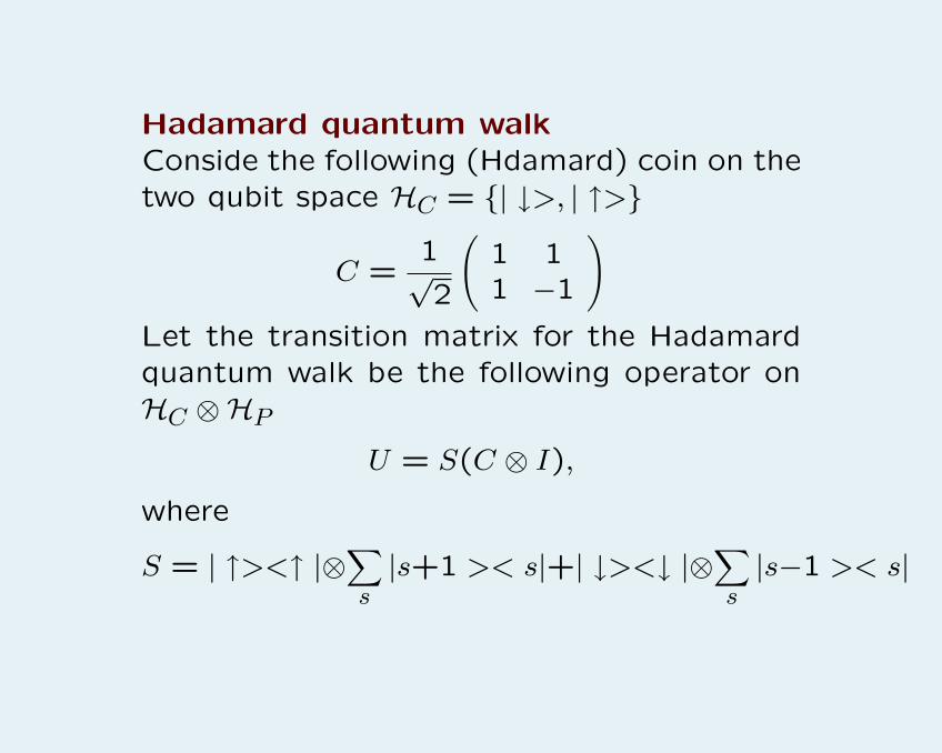
Hadamard quantum walkConside the following (Hdamard) coin on thetwo qubit space HC = {| ↓>, | ↑>}

C =1√2

(1 11 −1

)Let the transition matrix for the Hadamardquantum walk be the following operator onHC ⊗HP

U = S(C ⊗ I),

where

S = | ↑><↑ |⊗∑s|s+1 >< s|+| ↓><↓ |⊗

∑s|s−1 >< s|

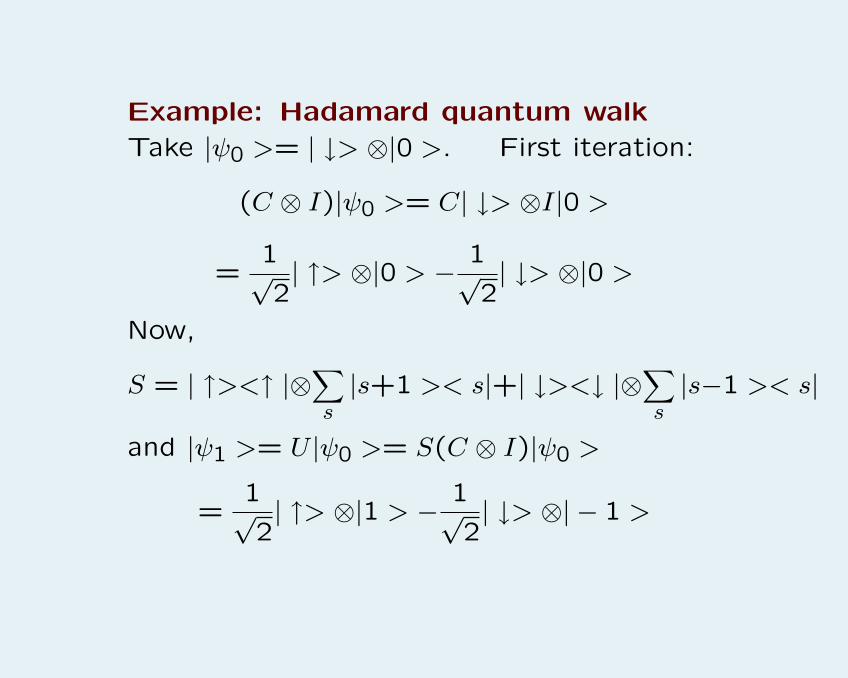
Example: Hadamard quantum walk

Take |ψ0 >= | ↓> ⊗|0 >. First iteration:

(C ⊗ I)|ψ0 >= C| ↓> ⊗I|0 >

=1√2| ↑> ⊗|0 > −

1√2| ↓> ⊗|0 >

Now,

S = | ↑><↑ |⊗∑s|s+1 >< s|+| ↓><↓ |⊗

∑s|s−1 >< s|

and |ψ1 >= U |ψ0 >= S(C ⊗ I)|ψ0 >

=1√2| ↑> ⊗|1 > −

1√2| ↓> ⊗| − 1 >

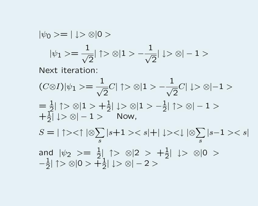
|ψ0 >= | ↓> ⊗|0 >

|ψ1 >=1√2| ↑> ⊗|1 > −

1√2| ↓> ⊗| − 1 >

Next iteration:

(C⊗I)|ψ1 >=1√2C| ↑> ⊗|1 > −

1√2C| ↓> ⊗|−1 >

= 12| ↑> ⊗|1 > +1

2| ↓> ⊗|1 > −12| ↑> ⊗| − 1 >

+12| ↓> ⊗| − 1 > Now,

S = | ↑><↑ |⊗∑s|s+1 >< s|+| ↓><↓ |⊗

∑s|s−1 >< s|

and |ψ2 >= 12| ↑> ⊗|2 > +1

2| ↓> ⊗|0 >

−12| ↑> ⊗|0 > +1

2| ↓> ⊗| − 2 >

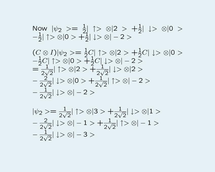
Now |ψ2 >= 12| ↑> ⊗|2 > +1

2| ↓> ⊗|0 >−1

2| ↑> ⊗|0 > +12| ↓> ⊗| − 2 >

(C ⊗ I)|ψ2 >= 12C| ↑> ⊗|2 > +1

2C| ↓> ⊗|0 >−1

2C| ↑> ⊗|0 > +12C| ↓> ⊗| − 2 >

= 12√

2| ↑> ⊗|2 > + 1

2√

2| ↓> ⊗|2 >

− 22√

2| ↓> ⊗|0 > + 1

2√

2| ↑> ⊗| − 2 >

− 12√

2| ↓> ⊗| − 2 >

|ψ2 >= 12√

2| ↑> ⊗|3 > + 1

2√

2| ↓> ⊗|1 >

− 22√

2| ↓> ⊗| − 1 > + 1

2√

2| ↑> ⊗| − 1 >

− 12√

2| ↓> ⊗| − 3 >

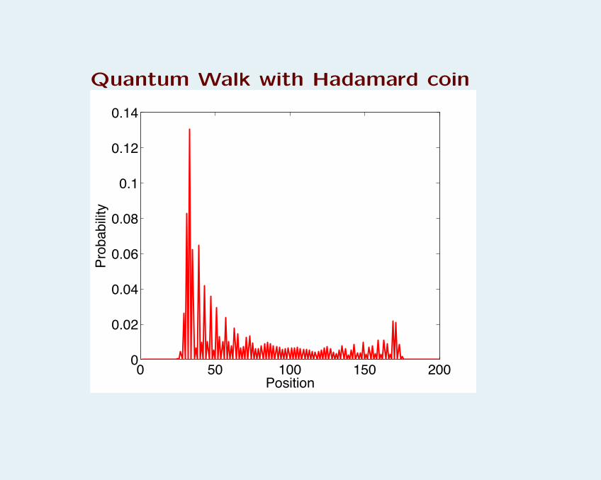
Quantum Walk with Hadamard coin

0 50 100 150 2000

0.02

0.04

0.06

0.08

0.1

0.12

0.14

Position

Probability

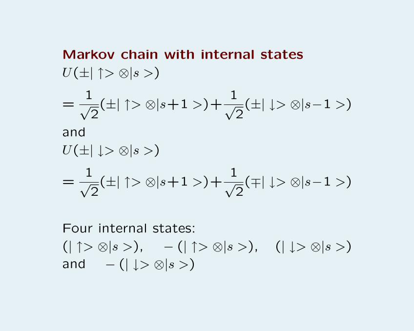
Markov chain with internal states

U(±| ↑> ⊗|s >)

=1√2(±| ↑> ⊗|s+1 >)+

1√2(±| ↓> ⊗|s−1 >)

and

U(±| ↓> ⊗|s >)

=1√2(±| ↑> ⊗|s+1 >)+

1√2(∓| ↓> ⊗|s−1 >)

Four internal states:

(| ↑> ⊗|s >), − (| ↑> ⊗|s >), (| ↓> ⊗|s >)

and − (| ↓> ⊗|s >)

Markov Chain

+|!> ⊗ |s >

- |!> ⊗ |s >

+ |"> ⊗ |s >

- |"> ⊗ |s >

Internal state

s

1

2

3

4

0-1-2 1 2 3

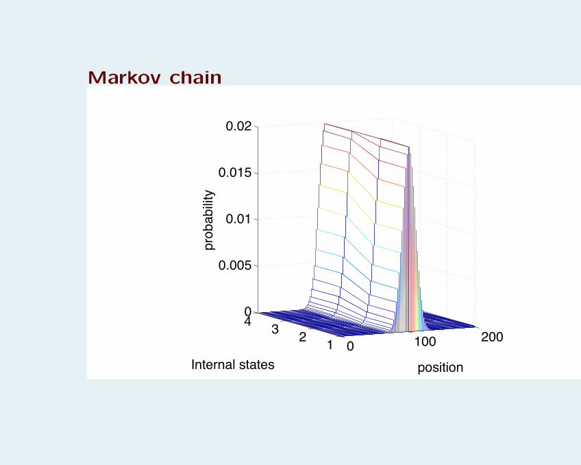
Markov chain

0 100 20012340

0.005

0.01

0.015

0.02

positionInternal states

prob

abilit

y

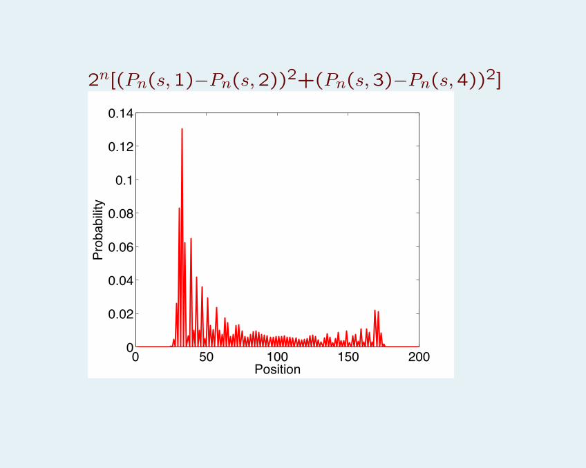
2n[(Pn(s,1)−Pn(s,2))2+(Pn(s,3)−Pn(s,4))2]

0 50 100 150 2000

0.02

0.04

0.06

0.08

0.1

0.12

0.14

Position

Probability

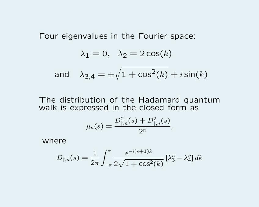
Four eigenvalues in the Fourier space:

λ1 = 0, λ2 = 2cos(k)

and λ3,4 = ±√

1 + cos2(k) + i sin(k)

The distribution of the Hadamard quantumwalk is expressed in the closed form as

µn(s) =D2↑,n(s) +D2

↓,n(s)

2n,

where

D↑,n(s) =1

2π

∫ π

−π

e−i(s+1)k

2√

1 + cos2(k)[λn3 − λn4] dk

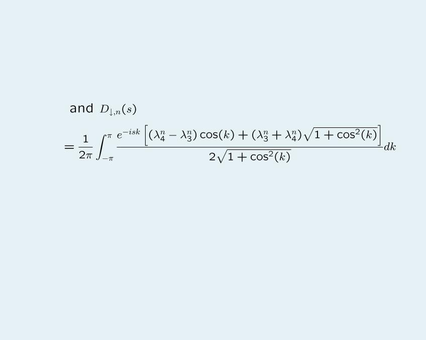
and D↓,n(s)

=1

2π

∫ π

−π

e−isk[(λn4 − λn3) cos(k) + (λn3 + λn4)

√1 + cos2(k)

]2√

1 + cos2(k)dk