The chromosphere above a -sunspot in the presence of fan ...Astronomy & Astrophysics manuscript no....

Astronomy & Astrophysics manuscript no. deltasp_arxiv c©ESO 2018November 8, 2018

The chromosphere above a δ-sunspot in the presence offan-shaped jets

Carolina Robustini1, Jorrit Leenaarts1, and Jaime de la Cruz Rodríguez1

Institute for Solar Physics, Department of Astronomy, Stockholm University, AlbaNova University Centre, SE-106 91 StockholmSweden e-mail: [email protected]

Received; accepted

ABSTRACT

Context. δ-sunspots are known to be favourable locations for fast and energetic events like flares and CMEs. The photosphere of thistype of sunspots has been thoroughly investigated in the past three decades. The atmospheric conditions in the chromosphere are notso well known, however.Aims. This study is focused on the chromosphere of a δ-sunspot that harbours a series of fan-shaped jets in its penumbra . The aimof this study is to establish the magnetic field topology and the temperature distribution in the presence of jets in the photosphere andthe chromosphere.Methods. We use data from the Swedish 1-m Solar Telescope (SST) and the Solar Dynamics Observatory. We invert the spectropo-larimetric FeI 6302 Å and Ca ii 8542 Å data from the SST using the the non-LTE inversion code NICOLE to estimate the magneticfield configuration, temperature and velocity structure in the chromosphere.Results. A loop-like magnetic structure is observed to emerge in the penumbra of the sunspot. The jets are launched from the loop-likestructure. Magnetic reconnection between this emerging field and the pre-existing vertical field is suggested by hot plasma patcheson the interface between the two fields. The height at which the reconnection takes place is located between log τ500 = −2 andlog τ500 = −3. The magnetic field vector and the atmospheric temperature maps show a stationary configuration during the wholeobservation.

Key words. Sunspots — Sun: chromosphere — Sun: photosphere — technique: Spectropolarimetry

1. Introduction

The chromosphere above sunspots exhibits many dynamic phe-nomena, such as umbral flashes, running penumbral waves, andvarious types of jets.

Chromospheric fan-shaped jets launched from sunspots havebeen reported by several authors (Roy 1973; Asai et al. 2001;Shimizu et al. 2009; Hou et al. 2016; Robustini et al. 2016; Liet al. 2016; Yang et al. 2016). From these previous observa-tions, we know that the length of these jets is of tens of Mm.They have an average velocity of 100-200 km s−1 and can lastfor more than one hour. They exhibit a sideways motion thathas been observed (Shibata et al. 1992; Savcheva et al. 2007)and simulated (Moreno-Insertis et al. 2008; Moreno-Insertis &Galsgaard 2013) also in anemone jets. The jets appear dark inHα and may exhibit a bright front in the EUV lines. In Shimizuet al. (2009) and Robustini et al. (2016) the jet footpoints appearbright in Ca ii H and Hα respectively. It has been suggested thatthe driver of this type of jets is magnetic reconnection and that,consequently, the bright footpoints are the result of local plasmaheating.

Jiang et al. (2011) have reproduced the structure of a fan-shaped jet in a 3D simulation of magnetic reconnection. The fanstructure that they simulate is caused by the sheared guide fieldlines that thread through the current sheet, and the jets are ac-celerated first by the magnetic pressure gradient and then by gaspressure gradients.

These jets are recurrently launched above sunspot structures.The majority (Roy 1973; Asai et al. 2001; Shimizu et al. 2009;

Robustini et al. 2016; Yang et al. 2016) have been reported onlight-bridges. There are nonetheless some exceptions. In one ofthe observations of Roy (1973) (MW 18594) the jets are rootedin the penumbra of a negative sunspot group harbouring a pos-itive polarity patch that weakens when jets start appearing. Inthe observations of Hou et al. (2016) the jets are launched froman apparent positive polarity field region between two distinctregular α-negative sunspots.

In this paper we report on fan-shaped jets observed in thepenumbra of a δ-sunspot. This kind of sunspot configurationconsists of umbrae of both polarities sharing the same penum-bra (Künzel 1960). δ-sunspots can harbour strong current densi-ties (Solanki 2003) and are often associated with flaring activity(Zirin & Liggett 1987; Sammis et al. 2000). It has been sug-gested that the complex topology of δ-sunspots originates fromthe emergence of twisted flux tubes (Tanaka 1991; Kurokawaet al. 2002). Takasao et al. (2015) simulated the formation of a δ-sunspot configuration from the emergence of an unstable kinkedflux tube which spontaneously develops into a quadrupole. Thefour polarities do not appear all together. First to appear is a mainpair. The arcade connecting the first pair expands and plasma ac-cumulates on its top. Eventually this leads to the submergence ofthe magnetic field and the appearance of a second pair of polari-ties between the main pair. The emerging flux tube employed byTakasao et al. (2015) had a single buoyant segment.

In addition, δ-sunspots have been simulated using two buoy-ant segments in a twisted flux emerging at the same time (Fang &Fan 2015). The submergence of the magnetic field predicted by

Article number, page 1 of 12

arX

iv:1

709.

0386

4v1

[as

tro-

ph.S

R]

12

Sep

2017

A&A proofs: manuscript no. deltasp_arxiv

these two model could find its observational proof in the down-flow observed at the PIL by Martinez Pillet et al. (1994).

Balthasar et al. (2014) and Jaeggli (2016) employed near-infrared spectropolarimetry to retrieve the magnetic and dynam-ical properties of δ-sunspots in the photosphere. Balthasar et al.(2014) report on the presence of an upflow aligned with the po-larity inversion line (PIL) of the spot and some photosphericbrightenings. Jaeggli (2016) found an intensification of the trans-verse magnetic field at the PIL. A similar intensification can alsobe found in Cristaldi et al. (2014). While the magnetic topol-ogy of δ-sunspots has been largely studied in the photosphere,we know very little about its configuration in the chromosphere.In this paper we will present the results of a study of the chro-mosphere above a δ-sunspot in the presence of fan-shaped jets,using polarimetric data inversion.

2. Observations and data reduction

The target of the observations is a δ-sunspot located in the activeregion NOAA 11791, observed on 2013 July 15 from 07:18 to08:24 UT. The coordinates in the middle of the time series are15.26◦ S, 16.69◦ E, with an observing angle of 27◦ (µ = 0.89).

Our observations were carried out at the Swedish 1-m SolarTelescope (SST, Scharmer et al. 2003) using the CRisp ImagingSpectroPolarimeter (CRISP, Scharmer et al. 2008) along threedifferent line profiles:

• Hα 6563 Å, at 13 positions between 6561.45 and 6564.55 Å,• Fe i 6301-6302 Å, at 18 positions between 6300.45 and

6302.10 Å,• Ca ii 8542 Å, at 21 positions between 8540.25 and

8543.75 Å.

The cadence between two complete profile scans along the sameprofile is 27 s. The pixel size and the spectral resolution at630 nm are 0′′.059 and R = λ/δλ ≈ 114000 respectively.

We recorded full Stokes vector data for Fe i 6301-6302 Å andCa ii 8542 Å. These lines, with effective Landé factor of 2.5 and1.1 respectively, are good diagnostic tools for the magnetic fieldin the photosphere (Fe i) and chromosphere (Ca ii). The CRISPdata reduction followed the pipeline described in de la CruzRodríguez et al. (2015) which includes image restoration withMulti-Object Multi-Frame Blind Deconvolution (MOMFBD,van Noort et al. 2005). In order to avoid degradation of thesignal-to-noise ratio from interpolation noise, the three datasetswere spatially aligned using as reference cube the Ca ii 8542 Ådata which has a weaker polarimetric signal compared to Fe i6301-6302 Å.

We also made use of co-observations of the Helioseismicand Magnetic Imager (HMI, Scherrer et al. 2012) and the Atmo-spheric Imaging Assembly (AIA, Lemen et al. 2012) on boardof the Solar Dynamics Observatory (SDO, Pesnell et al. 2012).

AIA data (with 12 s cadence) and HMI data (with 48 s ca-dence) have been aligned and resampled in space and time tomatch the cadence and pixel size of the SST data using the rou-tines developed by R. J. Rutten1. The alignment has been doneby first rotating the SDO subfield of interest to the same orienta-tion as the SST data. Then a cross correlation between the SSTHα wide-band and the HMI continuum data is performed. Theaccuracy of the co-alignment is on the order of an SDO pixelsize (0′′.5).1 http://www.staff.science.uu.nl/~rutte101/rridl/sdolib/

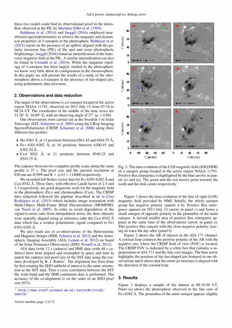
Fig. 1: The time evolution of the LOS magnetic field (SDO/HMI)of a sunspot group located in the active region NOAA 11791.Positive flux emergence is highlighted by the blue arrows in pan-els (c) and (e). The green and the red arrows point towards thenorth and the disk centre respectively.

Figure 1 shows the time evolution of the line of sight (LOS)magnetic field provided by HMI. Initally, the whole sunspotgroup has negative polarity (panels a–b). Positive flux emer-gence appears on 2013 July 14 (arrow in panel c) and forms asmall sunspot of opposite polarity in the penumbra of the mainsunspot. A second smaller area of positive flux emergence ap-pears at the same time of the observations (arrow in panel e).This positive flux cancels with the close negative polarity, leav-ing no trace the day after (panel f).

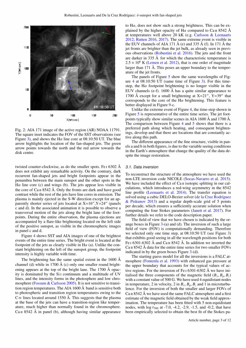
Figure 2 shows the AR of interest in the AIA 171 channel.A coronal loop connects the positive polarity of the AR with thenegative one, where the CRISP field of view (FOV) is located.The CRISP FOV is indicated by a white box that contains a su-perposition of AIA 171 and Hα line core images. The blue arrowhighlights the position of the fan-shaped jets featured in our ob-servations and it shows that the entire jet structure is aligned withthe direction of the coronal loop.

3. Results

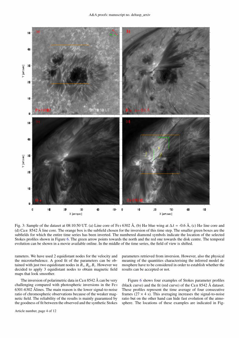
Figure 3 displays a sample of the dataset at 08:10:50 UT.Panel (a) shows the photosphere observed in the line core ofFe i 6302 Å. The penumbra of the main sunspot appears slightly


http://www.staff.science.uu.nl/~rutte101/rridl/sdolib/

http://www.staff.science.uu.nl/~rutte101/rridl/sdolib/

Robustini, Leenaarts and De la Cruz Rodríguez: δ-sunspot with fan-shaped jets

Fig. 2: AIA 171 image of the active region (AR) NOAA 11791.The square inset indicates the FOV of the SST observations (seeFigure 3), and shows the Hα line core at 08:10:50 UT. The bluearrow highlights the location of the fan-shaped jets. The greenarrow points towards the north and the red arrow towards thedisk centre.

twisted counter-clockwise, as do the smaller spots. Fe i 6302 Ådoes not exhibit any remarkable activity. On the contrary, darkrecurrent fan-shaped jets and bright footpoints appear in thepenumbra between the main sunspot and the other spots in theHα line core (c) and wings (b). The jets appear less visible inthe core of Ca ii 8542 Å. Only the fronts are dark and have goodcontrast while the rest of the jets have line cores in emission. Theplasma is mainly ejected in the S-W direction except for an ap-parently shorter series of jets located at X=16′′,Y=24′′ (panelsc and d). In the associated animation it is possible to observe atransversal motion of the jets along the bright lane of the foot-points. During the entire observation, the plasma ejections areaccompanied by a flare-like brightening located on the left sideof the positive sunspot, as visible in the chromospheric imagesin panel c and d.

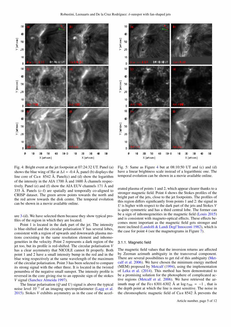
Figure 4 shows SST and AIA images of one of the brightestevents of the entire time series. The bright event is located at thefootpoint of the jets as clearly visible in Hα (a). Unlike the con-stant brightening on the left of the sunspot group, the footpointintensity is highly variable with time.

The brightening has the same spatial extent in the 1600 Åchannel (d) while in 1700 Å (c) only one smaller round bright-ening appears at the top of the bright lane. The 1700 Å opac-ity is dominated by the Si i continuum and a multitude of UVlines, and the intensity forms in the photosphere and low chro-mosphere (Fossum & Carlsson 2005). It is not sensitive to transi-tion region temperatures. The AIA 1600 Å band is sensitive bothto photospheric and transition region temperatures owing to theC iv lines located around 1550 Å. This suggests that the plasmaat the base of the jets can have a transition-region like temper-ature, much higher than normally found in the chromosphere.Ca ii 8542 Å in panel (b), although having similar appearance

to Hα, does not show such a strong brightness. This can be ex-plained by the higher opacity of Hα compared to Ca ii 8542 Åat temperatures well above 20 kK (e.g. Carlsson & Leenaarts2012; Rutten 2016, 2017). The same extreme event is visible inthe EUV channels of AIA 171 Å (e) and 335 Å (f). In 171 Å thejet fronts are brighter than the jet bulk, as already seen in previ-ous observations (Robustini et al. 2016). The jets and the frontare darker in 335 Å for which the characteristic temperature is2.5 × 106 K (Lemen et al. 2012), that is one order of magnitudelarger than 171 Å. This poses an upper boundary to the temper-ature of the jet fronts.

The panels of Figure 5 show the same wavelengths of Fig-ure 4 at 08:10:50 UT (same time of Figure 3). For this time-step, the Hα footpoint brightening is no longer visible in theEUV channels (e-f). 1600 Å has a quite similar appearance to1700 Å except for a small brightening at X=21′′, Y=39′′ thatcorresponds to the core of the Hα brightening. This feature isbetter displayed in Figure 9-c.

Unlike the extreme event of Figure 4, the time-step shown inFigure 5 is representative of the entire time series. The jet foot-points typically show similar scenes in AIA 1600 Å and 1700 Å.The comparison between Figure 4 and 5 shows that there is apreferred path along which heating, and consequent brighten-ings, develop and that there are locations that are constantly ac-tive along this path.

The different appearance of the fine structure, visible in pan-els a and b in both figures, is due to the variable seeing conditionsin the Earth’s atmosphere that change the quality of the data de-spite the image restoration.

3.1. Data inversion

To reconstruct the structure of the atmosphere we have used thenon-LTE inversion code NICOLE (Socas-Navarro et al. 2015).We have included the effect of Ca ii isotopic splitting in our cal-culations, which introduces a red-wing asymmetry in the 8542line profile (Leenaarts et al. 2014). The transfer equation issolved using a cubic DELO-Bezier solver (de la Cruz Rodríguez& Piskunov 2013) and a regular depth-scale grid of 5 pointsper decade, which ensures a sufficiently accurate solution whencomputing the four Stokes parameters (Janett et al. 2017). Forfurther details we refer to the code description paper.

The field of view that we have chosen is indicated by the or-ange boxes in Figure 3-(a) and (d). The inversion of such a largefield of view (FOV) is computationally demanding. Thereforewe selected only one time step, at 08:10:50 UT (see Figure 3)that exhibits good seeing in all the wavelength positions for bothFe i 6301-6302 Å and Ca ii 8542 Å. In addition we inverted theCa ii 8542 Å data for the entire time series for two smaller FOVsindicated in by the green boxes Figure 3-(d).

The starting guess model for all the inversions is a FALC at-mosphere (Fontenla et al. 1993) with enhanced gas pressure atthe upper boundary that accounts for the typical values of ac-tive regions. For the inversion of Fe i 6301-6302 Å we have ini-tialised the three components of the magnetic field (Bx, By, Bz)with a constant value of 500 G. We have used 4 equidistant nodesin temperature, 2 in velocity, 2 in Bx, By, Bz and 1 in microturbu-lence. For the inversion of both the smaller and larger FOVs ofCa ii 8542 Å we have used the same FALC atmosphere and a firstestimate of the magnetic field obtained by the weak field approx-imation. The temperature has been fitted with 5 non-equidistantnodes, with log τ500 at -7.0, -4.2, -2.9, -1.5, and -0.2, that havebeen empirically selected to obtain the best fit of the Stokes pa-



Fig. 3: Sample of the dataset at 08:10:50 UT. (a) Line core of Fe i 6302 Å, (b) Hα blue wing at ∆λ = -0.6 Å, (c) Hα line core and(d) Ca ii 8542 Å line core. The orange box is the subfield chosen for the inversion of this time step. The smaller green boxes are thesubfields for which the entire time series has been inverted. The numbered diamond symbols indicate the location of the selectedStokes profiles shown in Figure 6. The green arrow points towards the north and the red one towards the disk centre. The temporalevolution can be shown in a movie available online. In the middle of the time series, the field of view is shifted.

rameters. We have used 2 equidistant nodes for the velocity andthe microturbulence. A good fit of the parameters can be ob-tained with just two equidistant nodes in Bx, By, Bz. However wedecided to apply 3 equidistant nodes to obtain magnetic fieldmaps that look smoother.

The inversion of polarimetric data in Ca ii 8542 Å can be verychallenging compared with photospheric inversions in the Fe i6301-6302 Ålines. The main reason is the lower signal-to-noiseratio of chromospheric observations because of the weaker mag-netic field. The reliability of the results is mainly guaranteed bythe goodness of fit between the observed and the synthetic Stokes

parameters retrieved from inversion. However, also the physicalmeaning of the quantities characterising the inferred model at-mosphere have to be considered in order to establish whether theresults can be accepted or not.

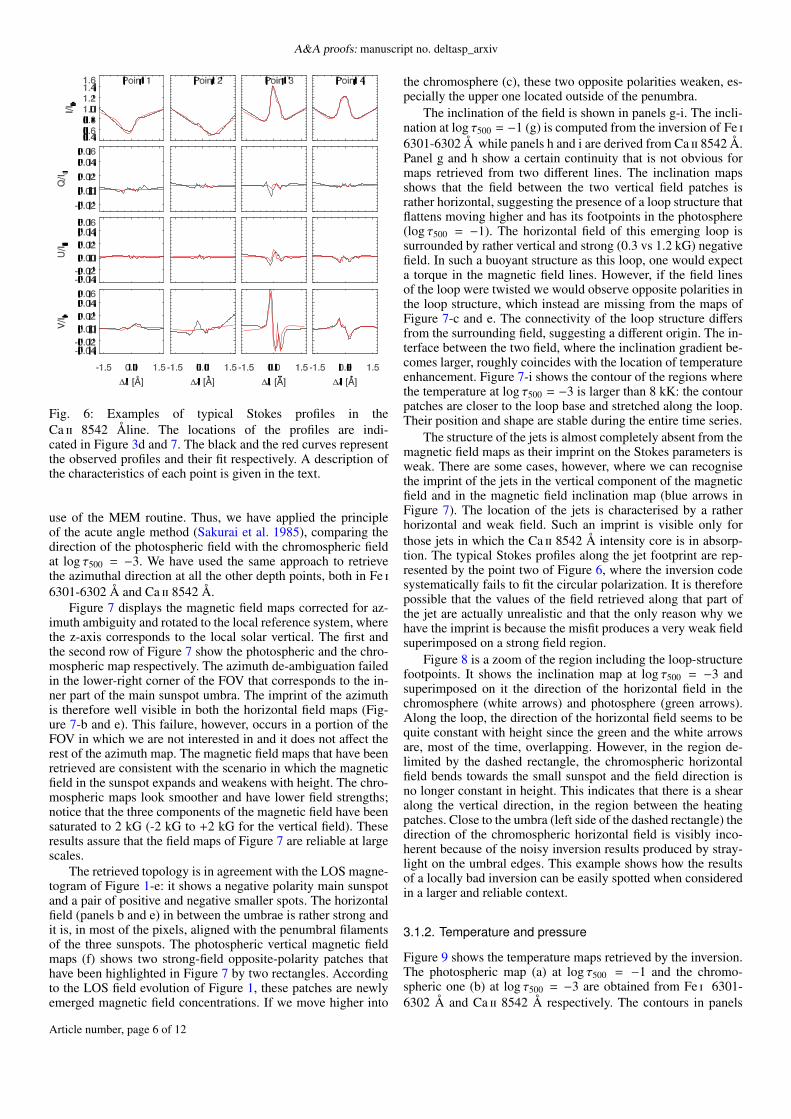
Figure 6 shows four examples of Stokes parameter profiles(black curve) and the fit (red curve) of the Ca ii 8542 Å dataset.These profiles represent the time average of four consecutiveframes (27 × 4 s). This averaging increases the signal-to-noiseratio but on the other hand can hide fast evolution of the atmo-sphere. The locations of these examples are indicated in Fig-



Fig. 4: Bright event at the jet footpoint at 07:24:32 UT. Panel (a)shows the blue wing of Hα at ∆λ = -0.4 Å, panel (b) displays theline core of Ca ii 8542 Å. Panel(c) and (d) show the logarithmof the intensity in the AIA 1700 Å and 1600 Å channels respec-tively. Panel (e) and (f) show the AIA EUV channels 171 Å and335 Å. Panels (c–f) are spatially and temporally co-aligned toCRISP dataset. The green arrow points towards the north andthe red arrow towards the disk centre. The temporal evolutioncan be shown in a movie available online.

ure 3-(d). We have selected them because they show typical pro-files of the region in which they are located.

Point 1 is located in the dark part of the jet. The intensityis blue-shifted and the circular polarisation V has several lobes,consistent with a region of upwards and downwards plasma mo-tions coexisting in the same resolution element and inhomo-geneities in the velocity. Point 2 represents a dark region of thejet too, but its profile is red-shifted. The circular polarisation Vhas a clear asymmetry that NICOLE cannot fit properly. Bothpoint 1 and 2 have a small intensity bump in the red and in theblue wing respectively at the same wavelength of the maximumof the circular polarisation. Point 3 has been selected to compareits strong signal with the other three. It is located in the twistedpenumbra of the negative small sunspot. The intensity profile isreversed in the core giving rise to an opposite sign of the stokesV signal (Sanchez Almeida 1997).

The linear polarisation (Q and U) signal is above the typicalnoise level 10−3 of an imaging spectropolarimeter (Lagg et al.2015). Stokes V exhibits asymmetry as in the case of the accel-

Fig. 5: Same as Figure 4 but at 08:10:50 UT and (c) and (d)have a linear brightness scale instead of a logarithmic one. Thetemporal evolution can be shown in a movie available online.

erated plasma of points 1 and 2, which appear clearer thanks to astronger magnetic field. Point 4 shows the Stokes profiles of thebright part of the jets, close to the jet footpoints. The profiles ofthis region differs significantly from points 1 and 2: the signal inU is higher with respect to the dark part of the jets and Stokes Vis quite symmetric and has a third central lobe. The former canbe a sign of inhomogeneities in the magnetic field (Louis 2015)and is consistent with magneto-optical effects. These effects be-comes more important as the magnetic field gets stronger andmore inclined (Landolfi & Landi Degl’Innocenti 1982), which isthe case for point 4 (see the magnetograms in Figure 7).

3.1.1. Magnetic field

The magnetic field values that the inversion returns are affectedby Zeeman azimuth ambiguity in the transversal component.There are several possibilities to get rid of this ambiguity (Met-calf et al. 2006). We have chosen the minimum energy method(MEM) proposed by Metcalf (1994), using the implementationof Leka et al. (2014). This method has been demonstrated tobe a promising solution for the photosphere of complicated ac-tive regions (Metcalf et al. 2006). We have retrieved the az-imuth map of the Fe i 6301-6302 Å at log τ500 = −1 , that isthe depth point at which the line is most sensitive. The noise inthe chromospheric magnetic field of Ca ii 8542 Å prevents the



Fig. 6: Examples of typical Stokes profiles in theCa ii 8542 Åline. The locations of the profiles are indi-cated in Figure 3d and 7. The black and the red curves representthe observed profiles and their fit respectively. A description ofthe characteristics of each point is given in the text.

use of the MEM routine. Thus, we have applied the principleof the acute angle method (Sakurai et al. 1985), comparing thedirection of the photospheric field with the chromospheric fieldat log τ500 = −3. We have used the same approach to retrievethe azimuthal direction at all the other depth points, both in Fe i6301-6302 Å and Ca ii 8542 Å.

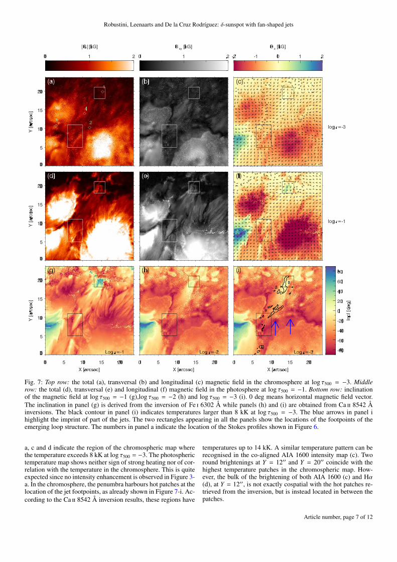
Figure 7 displays the magnetic field maps corrected for az-imuth ambiguity and rotated to the local reference system, wherethe z-axis corresponds to the local solar vertical. The first andthe second row of Figure 7 show the photospheric and the chro-mospheric map respectively. The azimuth de-ambiguation failedin the lower-right corner of the FOV that corresponds to the in-ner part of the main sunspot umbra. The imprint of the azimuthis therefore well visible in both the horizontal field maps (Fig-ure 7-b and e). This failure, however, occurs in a portion of theFOV in which we are not interested in and it does not affect therest of the azimuth map. The magnetic field maps that have beenretrieved are consistent with the scenario in which the magneticfield in the sunspot expands and weakens with height. The chro-mospheric maps look smoother and have lower field strengths;notice that the three components of the magnetic field have beensaturated to 2 kG (-2 kG to +2 kG for the vertical field). Theseresults assure that the field maps of Figure 7 are reliable at largescales.

The retrieved topology is in agreement with the LOS magne-togram of Figure 1-e: it shows a negative polarity main sunspotand a pair of positive and negative smaller spots. The horizontalfield (panels b and e) in between the umbrae is rather strong andit is, in most of the pixels, aligned with the penumbral filamentsof the three sunspots. The photospheric vertical magnetic fieldmaps (f) shows two strong-field opposite-polarity patches thathave been highlighted in Figure 7 by two rectangles. Accordingto the LOS field evolution of Figure 1, these patches are newlyemerged magnetic field concentrations. If we move higher into

the chromosphere (c), these two opposite polarities weaken, es-pecially the upper one located outside of the penumbra.

The inclination of the field is shown in panels g-i. The incli-nation at log τ500 = −1 (g) is computed from the inversion of Fe i6301-6302 Å while panels h and i are derived from Ca ii 8542 Å.Panel g and h show a certain continuity that is not obvious formaps retrieved from two different lines. The inclination mapsshows that the field between the two vertical field patches israther horizontal, suggesting the presence of a loop structure thatflattens moving higher and has its footpoints in the photosphere(log τ500 = −1). The horizontal field of this emerging loop issurrounded by rather vertical and strong (0.3 vs 1.2 kG) negativefield. In such a buoyant structure as this loop, one would expecta torque in the magnetic field lines. However, if the field linesof the loop were twisted we would observe opposite polarities inthe loop structure, which instead are missing from the maps ofFigure 7-c and e. The connectivity of the loop structure differsfrom the surrounding field, suggesting a different origin. The in-terface between the two field, where the inclination gradient be-comes larger, roughly coincides with the location of temperatureenhancement. Figure 7-i shows the contour of the regions wherethe temperature at log τ500 = −3 is larger than 8 kK: the contourpatches are closer to the loop base and stretched along the loop.Their position and shape are stable during the entire time series.

The structure of the jets is almost completely absent from themagnetic field maps as their imprint on the Stokes parameters isweak. There are some cases, however, where we can recognisethe imprint of the jets in the vertical component of the magneticfield and in the magnetic field inclination map (blue arrows inFigure 7). The location of the jets is characterised by a ratherhorizontal and weak field. Such an imprint is visible only forthose jets in which the Ca ii 8542 Å intensity core is in absorp-tion. The typical Stokes profiles along the jet footprint are rep-resented by the point two of Figure 6, where the inversion codesystematically fails to fit the circular polarization. It is thereforepossible that the values of the field retrieved along that part ofthe jet are actually unrealistic and that the only reason why wehave the imprint is because the misfit produces a very weak fieldsuperimposed on a strong field region.

Figure 8 is a zoom of the region including the loop-structurefootpoints. It shows the inclination map at log τ500 = −3 andsuperimposed on it the direction of the horizontal field in thechromosphere (white arrows) and photosphere (green arrows).Along the loop, the direction of the horizontal field seems to bequite constant with height since the green and the white arrowsare, most of the time, overlapping. However, in the region de-limited by the dashed rectangle, the chromospheric horizontalfield bends towards the small sunspot and the field direction isno longer constant in height. This indicates that there is a shearalong the vertical direction, in the region between the heatingpatches. Close to the umbra (left side of the dashed rectangle) thedirection of the chromospheric horizontal field is visibly inco-herent because of the noisy inversion results produced by stray-light on the umbral edges. This example shows how the resultsof a locally bad inversion can be easily spotted when consideredin a larger and reliable context.

3.1.2. Temperature and pressure

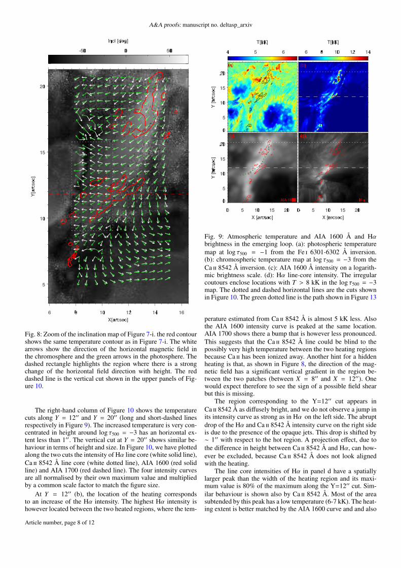
Figure 9 shows the temperature maps retrieved by the inversion.The photospheric map (a) at log τ500 = −1 and the chromo-spheric one (b) at log τ500 = −3 are obtained from Fe i 6301-6302 Å and Ca ii 8542 Å respectively. The contours in panels



Fig. 7: Top row: the total (a), transversal (b) and longitudinal (c) magnetic field in the chromosphere at log τ500 = −3. Middlerow: the total (d), transversal (e) and longitudinal (f) magnetic field in the photosphere at log τ500 = −1. Bottom row: inclinationof the magnetic field at log τ500 = −1 (g),log τ500 = −2 (h) and log τ500 = −3 (i). 0 deg means horizontal magnetic field vector.The inclination in panel (g) is derived from the inversion of Fe i 6302 Å while panels (h) and (i) are obtained from Ca ii 8542 Åinversions. The black contour in panel (i) indicates temperatures larger than 8 kK at log τ500 = −3. The blue arrows in panel ihighlight the imprint of part of the jets. The two rectangles appearing in all the panels show the locations of the footpoints of theemerging loop structure. The numbers in panel a indicate the location of the Stokes profiles shown in Figure 6.

a, c and d indicate the region of the chromospheric map wherethe temperature exceeds 8 kK at log τ500 = −3. The photospherictemperature map shows neither sign of strong heating nor of cor-relation with the temperature in the chromosphere. This is quiteexpected since no intensity enhancement is observed in Figure 3-a. In the chromosphere, the penumbra harbours hot patches at thelocation of the jet footpoints, as already shown in Figure 7-i. Ac-cording to the Ca ii 8542 Å inversion results, these regions have

temperatures up to 14 kK. A similar temperature pattern can berecognised in the co-aligned AIA 1600 intensity map (c). Tworound brightenings at Y = 12′′ and Y = 20′′ coincide with thehighest temperature patches in the chromospheric map. How-ever, the bulk of the brightening of both AIA 1600 (c) and Hα(d), at Y = 12′′, is not exactly cospatial with the hot patches re-trieved from the inversion, but is instead located in between thepatches.



Fig. 8: Zoom of the inclination map of Figure 7-i. the red contourshows the same temperature contour as in Figure 7-i. The whitearrows show the direction of the horizontal magnetic field inthe chromosphere and the green arrows in the photosphere. Thedashed rectangle highlights the region where there is a strongchange of the horizontal field direction with height. The reddashed line is the vertical cut shown in the upper panels of Fig-ure 10.

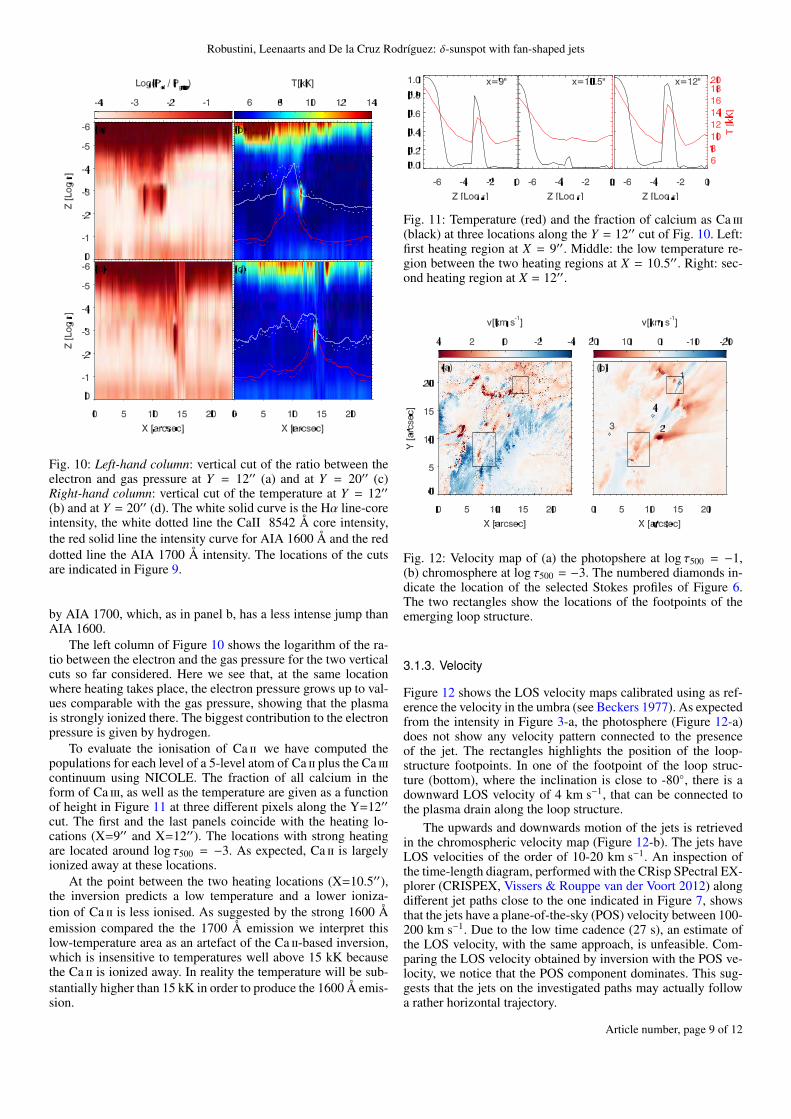
The right-hand column of Figure 10 shows the temperaturecuts along Y = 12′′ and Y = 20′′ (long and short-dashed linesrespectively in Figure 9). The increased temperature is very con-centrated in height around log τ500 = −3 has an horizontal ex-tent less than 1′′. The vertical cut at Y = 20′′ shows similar be-haviour in terms of height and size. In Figure 10, we have plottedalong the two cuts the intensity of Hα line core (white solid line),Ca ii 8542 Å line core (white dotted line), AIA 1600 (red solidline) and AIA 1700 (red dashed line). The four intensity curvesare all normalised by their own maximum value and multipliedby a common scale factor to match the figure size.

At Y = 12′′ (b), the location of the heating correspondsto an increase of the Hα intensity. The highest Hα intensity ishowever located between the two heated regions, where the tem-

Fig. 9: Atmospheric temperature and AIA 1600 Å and Hαbrightness in the emerging loop. (a): photospheric temperaturemap at log τ500 = −1 from the Fe i 6301-6302 Å inversion.(b): chromospheric temperature map at log τ500 = −3 from theCa ii 8542 Å inversion. (c): AIA 1600 Å intensity on a logarith-mic brightness scale. (d): Hα line-core intensity. The irregularcoutours enclose locations with T > 8 kK in the log τ500 = −3map. The dotted and dashed horizontal lines are the cuts shownin Figure 10. The green dotted line is the path shown in Figure 13

perature estimated from Ca ii 8542 Å is almost 5 kK less. Alsothe AIA 1600 intensity curve is peaked at the same location.AIA 1700 shows there a bump that is however less pronounced.This suggests that the Ca ii 8542 Å line could be blind to thepossibly very high temperature between the two heating regionsbecause Ca ii has been ionized away. Another hint for a hiddenheating is that, as shown in Figure 8, the direction of the mag-netic field has a significant vertical gradient in the region be-tween the two patches (between X = 8′′ and X = 12′′). Onewould expect therefore to see the sign of a possible field shearbut this is missing.

The region corresponding to the Y=12′′ cut appears inCa ii 8542 Å as diffusely bright, and we do not observe a jump inits intensity curve as strong as in Hα on the left side. The abruptdrop of the Hα and Ca ii 8542 Å intensity curve on the right sideis due to the presence of the opaque jets. This drop is shifted by∼ 1′′ with respect to the hot region. A projection effect, due tothe difference in height between Ca ii 8542 Å and Hα, can how-ever be excluded, because Ca ii 8542 Å does not look alignedwith the heating.

The line core intensities of Hα in panel d have a spatiallylarger peak than the width of the heating region and its maxi-mum value is 80% of the maximum along the Y=12′′ cut. Sim-ilar behaviour is shown also by Ca ii 8542 Å. Most of the areasubtended by this peak has a low temperature (6-7 kK). The heat-ing extent is better matched by the AIA 1600 curve and and also



Fig. 10: Left-hand column: vertical cut of the ratio between theelectron and gas pressure at Y = 12′′ (a) and at Y = 20′′ (c)Right-hand column: vertical cut of the temperature at Y = 12′′(b) and at Y = 20′′ (d). The white solid curve is the Hα line-coreintensity, the white dotted line the CaII 8542 Å core intensity,the red solid line the intensity curve for AIA 1600 Å and the reddotted line the AIA 1700 Å intensity. The locations of the cutsare indicated in Figure 9.

by AIA 1700, which, as in panel b, has a less intense jump thanAIA 1600.

The left column of Figure 10 shows the logarithm of the ra-tio between the electron and the gas pressure for the two verticalcuts so far considered. Here we see that, at the same locationwhere heating takes place, the electron pressure grows up to val-ues comparable with the gas pressure, showing that the plasmais strongly ionized there. The biggest contribution to the electronpressure is given by hydrogen.

To evaluate the ionisation of Ca ii we have computed thepopulations for each level of a 5-level atom of Ca ii plus the Ca iiicontinuum using NICOLE. The fraction of all calcium in theform of Ca iii, as well as the temperature are given as a functionof height in Figure 11 at three different pixels along the Y=12′′cut. The first and the last panels coincide with the heating lo-cations (X=9′′ and X=12′′). The locations with strong heatingare located around log τ500 = −3. As expected, Ca ii is largelyionized away at these locations.

At the point between the two heating locations (X=10.5′′),the inversion predicts a low temperature and a lower ioniza-tion of Ca ii is less ionised. As suggested by the strong 1600 Åemission compared the the 1700 Å emission we interpret thislow-temperature area as an artefact of the Ca ii-based inversion,which is insensitive to temperatures well above 15 kK becausethe Ca ii is ionized away. In reality the temperature will be sub-stantially higher than 15 kK in order to produce the 1600 Å emis-sion.

Fig. 11: Temperature (red) and the fraction of calcium as Ca iii(black) at three locations along the Y = 12′′ cut of Fig. 10. Left:first heating region at X = 9′′. Middle: the low temperature re-gion between the two heating regions at X = 10.5′′. Right: sec-ond heating region at X = 12′′.

Fig. 12: Velocity map of (a) the photopshere at log τ500 = −1,(b) chromosphere at log τ500 = −3. The numbered diamonds in-dicate the location of the selected Stokes profiles of Figure 6.The two rectangles show the locations of the footpoints of theemerging loop structure.

3.1.3. Velocity

Figure 12 shows the LOS velocity maps calibrated using as ref-erence the velocity in the umbra (see Beckers 1977). As expectedfrom the intensity in Figure 3-a, the photosphere (Figure 12-a)does not show any velocity pattern connected to the presenceof the jet. The rectangles highlights the position of the loop-structure footpoints. In one of the footpoint of the loop struc-ture (bottom), where the inclination is close to -80◦, there is adownward LOS velocity of 4 km s−1, that can be connected tothe plasma drain along the loop structure.

The upwards and downwards motion of the jets is retrievedin the chromospheric velocity map (Figure 12-b). The jets haveLOS velocities of the order of 10-20 km s−1. An inspection ofthe time-length diagram, performed with the CRisp SPectral EX-plorer (CRISPEX, Vissers & Rouppe van der Voort 2012) alongdifferent jet paths close to the one indicated in Figure 7, showsthat the jets have a plane-of-the-sky (POS) velocity between 100-200 km s−1. Due to the low time cadence (27 s), an estimate ofthe LOS velocity, with the same approach, is unfeasible. Com-paring the LOS velocity obtained by inversion with the POS ve-locity, we notice that the POS component dominates. This sug-gests that the jets on the investigated paths may actually followa rather horizontal trajectory.



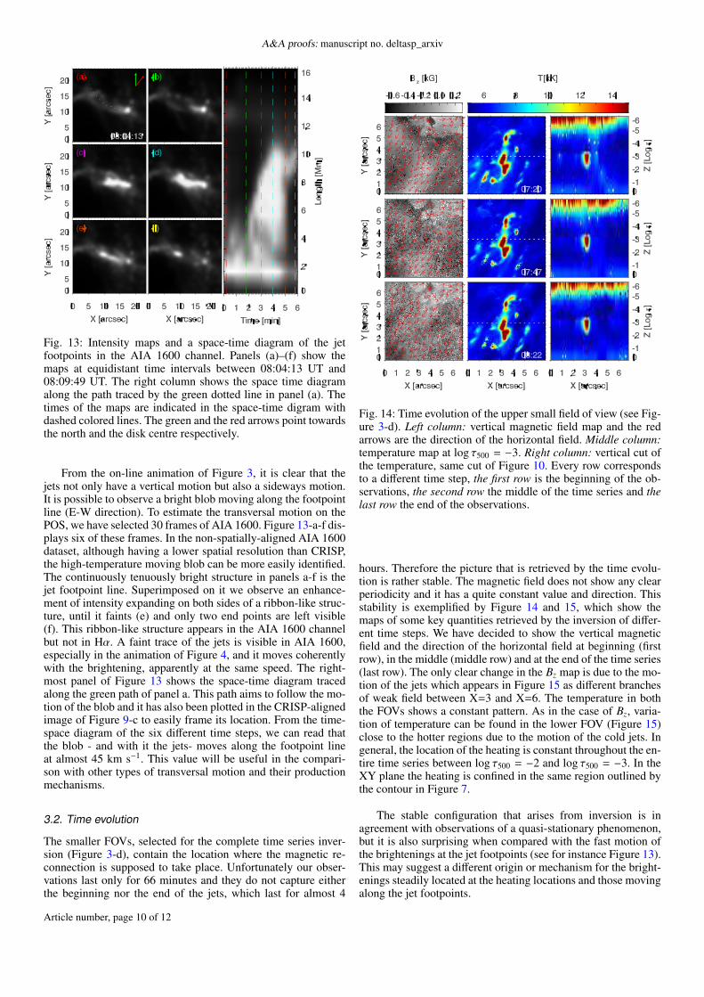
Fig. 13: Intensity maps and a space-time diagram of the jetfootpoints in the AIA 1600 channel. Panels (a)–(f) show themaps at equidistant time intervals between 08:04:13 UT and08:09:49 UT. The right column shows the space time diagramalong the path traced by the green dotted line in panel (a). Thetimes of the maps are indicated in the space-time digram withdashed colored lines. The green and the red arrows point towardsthe north and the disk centre respectively.

From the on-line animation of Figure 3, it is clear that thejets not only have a vertical motion but also a sideways motion.It is possible to observe a bright blob moving along the footpointline (E-W direction). To estimate the transversal motion on thePOS, we have selected 30 frames of AIA 1600. Figure 13-a-f dis-plays six of these frames. In the non-spatially-aligned AIA 1600dataset, although having a lower spatial resolution than CRISP,the high-temperature moving blob can be more easily identified.The continuously tenuously bright structure in panels a-f is thejet footpoint line. Superimposed on it we observe an enhance-ment of intensity expanding on both sides of a ribbon-like struc-ture, until it faints (e) and only two end points are left visible(f). This ribbon-like structure appears in the AIA 1600 channelbut not in Hα. A faint trace of the jets is visible in AIA 1600,especially in the animation of Figure 4, and it moves coherentlywith the brightening, apparently at the same speed. The right-most panel of Figure 13 shows the space-time diagram tracedalong the green path of panel a. This path aims to follow the mo-tion of the blob and it has also been plotted in the CRISP-alignedimage of Figure 9-c to easily frame its location. From the time-space diagram of the six different time steps, we can read thatthe blob - and with it the jets- moves along the footpoint lineat almost 45 km s−1. This value will be useful in the compari-son with other types of transversal motion and their productionmechanisms.

3.2. Time evolution

The smaller FOVs, selected for the complete time series inver-sion (Figure 3-d), contain the location where the magnetic re-connection is supposed to take place. Unfortunately our obser-vations last only for 66 minutes and they do not capture eitherthe beginning nor the end of the jets, which last for almost 4

Fig. 14: Time evolution of the upper small field of view (see Fig-ure 3-d). Left column: vertical magnetic field map and the redarrows are the direction of the horizontal field. Middle column:temperature map at log τ500 = −3. Right column: vertical cut ofthe temperature, same cut of Figure 10. Every row correspondsto a different time step, the first row is the beginning of the ob-servations, the second row the middle of the time series and thelast row the end of the observations.

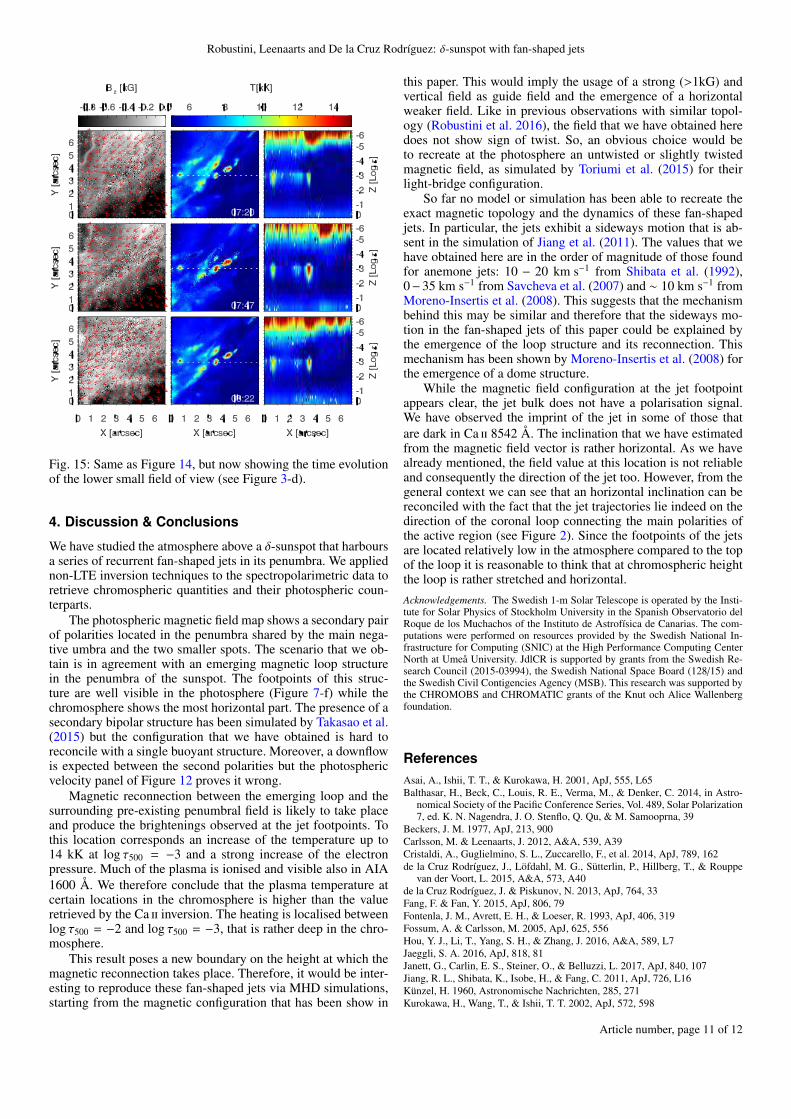
hours. Therefore the picture that is retrieved by the time evolu-tion is rather stable. The magnetic field does not show any clearperiodicity and it has a quite constant value and direction. Thisstability is exemplified by Figure 14 and 15, which show themaps of some key quantities retrieved by the inversion of differ-ent time steps. We have decided to show the vertical magneticfield and the direction of the horizontal field at beginning (firstrow), in the middle (middle row) and at the end of the time series(last row). The only clear change in the Bz map is due to the mo-tion of the jets which appears in Figure 15 as different branchesof weak field between X=3 and X=6. The temperature in boththe FOVs shows a constant pattern. As in the case of Bz, varia-tion of temperature can be found in the lower FOV (Figure 15)close to the hotter regions due to the motion of the cold jets. Ingeneral, the location of the heating is constant throughout the en-tire time series between log τ500 = −2 and log τ500 = −3. In theXY plane the heating is confined in the same region outlined bythe contour in Figure 7.

The stable configuration that arises from inversion is inagreement with observations of a quasi-stationary phenomenon,but it is also surprising when compared with the fast motion ofthe brightenings at the jet footpoints (see for instance Figure 13).This may suggest a different origin or mechanism for the bright-enings steadily located at the heating locations and those movingalong the jet footpoints.



Fig. 15: Same as Figure 14, but now showing the time evolutionof the lower small field of view (see Figure 3-d).

4. Discussion & Conclusions

We have studied the atmosphere above a δ-sunspot that harboursa series of recurrent fan-shaped jets in its penumbra. We appliednon-LTE inversion techniques to the spectropolarimetric data toretrieve chromospheric quantities and their photospheric coun-terparts.

The photospheric magnetic field map shows a secondary pairof polarities located in the penumbra shared by the main nega-tive umbra and the two smaller spots. The scenario that we ob-tain is in agreement with an emerging magnetic loop structurein the penumbra of the sunspot. The footpoints of this struc-ture are well visible in the photosphere (Figure 7-f) while thechromosphere shows the most horizontal part. The presence of asecondary bipolar structure has been simulated by Takasao et al.(2015) but the configuration that we have obtained is hard toreconcile with a single buoyant structure. Moreover, a downflowis expected between the second polarities but the photosphericvelocity panel of Figure 12 proves it wrong.

Magnetic reconnection between the emerging loop and thesurrounding pre-existing penumbral field is likely to take placeand produce the brightenings observed at the jet footpoints. Tothis location corresponds an increase of the temperature up to14 kK at log τ500 = −3 and a strong increase of the electronpressure. Much of the plasma is ionised and visible also in AIA1600 Å. We therefore conclude that the plasma temperature atcertain locations in the chromosphere is higher than the valueretrieved by the Ca ii inversion. The heating is localised betweenlog τ500 = −2 and log τ500 = −3, that is rather deep in the chro-mosphere.

This result poses a new boundary on the height at which themagnetic reconnection takes place. Therefore, it would be inter-esting to reproduce these fan-shaped jets via MHD simulations,starting from the magnetic configuration that has been show in

this paper. This would imply the usage of a strong (>1kG) andvertical field as guide field and the emergence of a horizontalweaker field. Like in previous observations with similar topol-ogy (Robustini et al. 2016), the field that we have obtained heredoes not show sign of twist. So, an obvious choice would beto recreate at the photosphere an untwisted or slightly twistedmagnetic field, as simulated by Toriumi et al. (2015) for theirlight-bridge configuration.

So far no model or simulation has been able to recreate theexact magnetic topology and the dynamics of these fan-shapedjets. In particular, the jets exhibit a sideways motion that is ab-sent in the simulation of Jiang et al. (2011). The values that wehave obtained here are in the order of magnitude of those foundfor anemone jets: 10 − 20 km s−1 from Shibata et al. (1992),0−35 km s−1 from Savcheva et al. (2007) and ∼ 10 km s−1 fromMoreno-Insertis et al. (2008). This suggests that the mechanismbehind this may be similar and therefore that the sideways mo-tion in the fan-shaped jets of this paper could be explained bythe emergence of the loop structure and its reconnection. Thismechanism has been shown by Moreno-Insertis et al. (2008) forthe emergence of a dome structure.

While the magnetic field configuration at the jet footpointappears clear, the jet bulk does not have a polarisation signal.We have observed the imprint of the jet in some of those thatare dark in Ca ii 8542 Å. The inclination that we have estimatedfrom the magnetic field vector is rather horizontal. As we havealready mentioned, the field value at this location is not reliableand consequently the direction of the jet too. However, from thegeneral context we can see that an horizontal inclination can bereconciled with the fact that the jet trajectories lie indeed on thedirection of the coronal loop connecting the main polarities ofthe active region (see Figure 2). Since the footpoints of the jetsare located relatively low in the atmosphere compared to the topof the loop it is reasonable to think that at chromospheric heightthe loop is rather stretched and horizontal.

Acknowledgements. The Swedish 1-m Solar Telescope is operated by the Insti-tute for Solar Physics of Stockholm University in the Spanish Observatorio delRoque de los Muchachos of the Instituto de Astrofísica de Canarias. The com-putations were performed on resources provided by the Swedish National In-frastructure for Computing (SNIC) at the High Performance Computing CenterNorth at Umeå University. JdlCR is supported by grants from the Swedish Re-search Council (2015-03994), the Swedish National Space Board (128/15) andthe Swedish Civil Contigencies Agency (MSB). This research was supported bythe CHROMOBS and CHROMATIC grants of the Knut och Alice Wallenbergfoundation.

ReferencesAsai, A., Ishii, T. T., & Kurokawa, H. 2001, ApJ, 555, L65Balthasar, H., Beck, C., Louis, R. E., Verma, M., & Denker, C. 2014, in Astro-

nomical Society of the Pacific Conference Series, Vol. 489, Solar Polarization7, ed. K. N. Nagendra, J. O. Stenflo, Q. Qu, & M. Samooprna, 39

Beckers, J. M. 1977, ApJ, 213, 900Carlsson, M. & Leenaarts, J. 2012, A&A, 539, A39Cristaldi, A., Guglielmino, S. L., Zuccarello, F., et al. 2014, ApJ, 789, 162de la Cruz Rodríguez, J., Löfdahl, M. G., Sütterlin, P., Hillberg, T., & Rouppe

van der Voort, L. 2015, A&A, 573, A40de la Cruz Rodríguez, J. & Piskunov, N. 2013, ApJ, 764, 33Fang, F. & Fan, Y. 2015, ApJ, 806, 79Fontenla, J. M., Avrett, E. H., & Loeser, R. 1993, ApJ, 406, 319Fossum, A. & Carlsson, M. 2005, ApJ, 625, 556Hou, Y. J., Li, T., Yang, S. H., & Zhang, J. 2016, A&A, 589, L7Jaeggli, S. A. 2016, ApJ, 818, 81Janett, G., Carlin, E. S., Steiner, O., & Belluzzi, L. 2017, ApJ, 840, 107Jiang, R. L., Shibata, K., Isobe, H., & Fang, C. 2011, ApJ, 726, L16Künzel, H. 1960, Astronomische Nachrichten, 285, 271Kurokawa, H., Wang, T., & Ishii, T. T. 2002, ApJ, 572, 598



Lagg, A., Lites, B., Harvey, J., Gosain, S., & Centeno, R. 2015,Space Sci. Rev.[arXiv:1510.06865]

Landolfi, M. & Landi Degl’Innocenti, E. 1982, Sol. Phys., 78, 355Leenaarts, J., de la Cruz Rodríguez, J., Kochukhov, O., & Carlsson, M. 2014,

ApJ, 784, L17Leka, K. D., Barnes, G., & Crouch, A. 2014, AMBIG: Automated Ambiguity-

Resolution Code, Astrophysics Source Code LibraryLemen, J. R., Title, A. M., Akin, D. J., et al. 2012, Sol. Phys., 275, 17Li, Z., Fang, C., Guo, Y., et al. 2016, ApJ, 826, 217Louis, R. E. 2015, Advances in Space Research, 56, 2305Martinez Pillet, V., Lites, B. W., Skumanich, A., & Degenhardt, D. 1994, ApJ,

425, L113Metcalf, T. R. 1994, Sol. Phys., 155, 235Metcalf, T. R., Leka, K. D., Barnes, G., et al. 2006, Sol. Phys., 237, 267Moreno-Insertis, F. & Galsgaard, K. 2013, ApJ, 771, 20Moreno-Insertis, F., Galsgaard, K., & Ugarte-Urra, I. 2008, ApJ, 673, L211Pesnell, W. D., Thompson, B. J., & Chamberlin, P. C. 2012, Sol. Phys., 275, 3Robustini, C., Leenaarts, J., de la Cruz Rodriguez, J., & Rouppe van der Voort,

L. 2016, A&A, 590, A57Roy, J.-R. 1973, Sol. Phys., 32, 139Rutten, R. J. 2016, A&A, 590, A124Rutten, R. J. 2017, A&A, 598, A89Sakurai, T., Makita, M., & Shibasaki, K. 1985, in Theo. Prob. High Resolution

Solar Physics, ed. H. U. Schmidt, 313Sammis, I., Tang, F., & Zirin, H. 2000, ApJ, 540, 583Sanchez Almeida, J. 1997, A&A, 324, 763Savcheva, A., Cirtain, J., Deluca, E. E., et al. 2007, PASJ, 59, S771Scharmer, G. B., Bjelksjo, K., Korhonen, T. K., Lindberg, B., & Petterson, B.

2003, in Proc. SPIE, Vol. 4853, Innovative Telescopes and Instrumentationfor Solar Astrophysics, ed. S. L. Keil & S. V. Avakyan, 341–350

Scharmer, G. B., Narayan, G., Hillberg, T., et al. 2008, ApJ, 689, L69Scherrer, P. H., Schou, J., Bush, R. I., et al. 2012, Sol. Phys., 275, 207Shibata, K., Ishido, Y., Acton, L. W., et al. 1992, PASJ, 44, L173Shimizu, T., Katsukawa, Y., Kubo, M., et al. 2009, ApJ, 696, L66Socas-Navarro, H., de la Cruz Rodríguez, J., Asensio Ramos, A., Trujillo Bueno,

J., & Ruiz Cobo, B. 2015, A&A, 577, A7Solanki, S. K. 2003, A&A Rev., 11, 153Takasao, S., Fan, Y., Cheung, M. C. M., & Shibata, K. 2015, ApJ, 813, 112Tanaka, K. 1991, Sol. Phys., 136, 133Toriumi, S., Cheung, M. C. M., & Katsukawa, Y. 2015, ApJ, 811, 138van Noort, M., Rouppe van der Voort, L., & Löfdahl, M. G. 2005, Sol. Phys.,

228, 191Vissers, G. & Rouppe van der Voort, L. 2012, ApJ, 750, 22Yang, S., Zhang, J., & Erdélyi, R. 2016, ApJ, 833, L18Zirin, H. & Liggett, M. A. 1987, Sol. Phys., 113, 267


The chromosphere above a -sunspot in the presence of fan ...Astronomy & Astrophysics manuscript no....

Documents

Transcript of The chromosphere above a -sunspot in the presence of fan ...Astronomy & Astrophysics manuscript no....