LNF - 10/14(P)April 13, 2010

Technical Design Report of the γγ Taggers for the

KLOE-2 Experiment

The KLOE-2 Collaboration

G. De Robertis, O. Erriquez, F. Loddo, A. Ranieri,Dipartimento di Fisica, Universita di Bari and INFN sezione di Bari, Bari, Italy

G. Morello, M. Schioppa, S. Stucci,Dipartimento di Fisica, Universita della Calabria and INFN gruppo collegato di Cosenza,

Cosenza, Italy

E. Czerwinski, P. Moskal, M. Silarski, J. ZdebikInstitute of Physics, Jagellonian University, Cracow, Poland

D. Babusci, G. Bencivenni, C. Bloise, F. Bossi, P. Campana, G. Capon, P. Ciambrone,E. Dane, E. De Lucia, D. Domenici, G. Felici, S. Giovannella, F. Happacher, E. Iarocci,

M. Jacewicz, J. Lee-Franzini, M. Martini, S. Miscetti, L. Quintieri, V. Patera, P. Santangelo,I. Sarra, B. Sciascia, A. Sciubba, G. Venanzoni, R. VersaciLaboratori Nazionali di Frascati dell’ INFN, Frascati, Italy

S. A. Bulychjev, V. V. Kulikov, M. A. Martemianov, M. A. MatsyukInstitute for Theoretical and Experimental Physics (ITEP), Moscow, Russia

C. Di DonatoDipartimento di Scienze Fisiche, Universita di Napoli “Federico II” and INFN sezione di

Napoli, Napoli, Italy

C. Bini, V. Bocci, A. De Santis, G. De Zorzi, A. Di Domenico, S. Fiore, P. Franzini, P. GauzziDipartimento di Fisica, “Sapienza” Universita di Roma and INFN sezione di Roma, Roma,

Italy

F. Archilli, D. Badoni, F. Gonnella, R. Messi, D. MoriccianiDipartimento di Fisica, Universita di Roma “Tor Vergata” and INFN sezione di Roma 2,

Roma, Italy

P. Branchini, A. Budano, F. Ceradini, B. Di Micco, E. Graziani, F. Nguyen, A. Passeri,C. Taccini, L. Tortora

Dipartimento di Fisica, Universita Roma Tre and INFN sezione di Roma Tre, Roma, Italy

B. Hoistad, T. Johansson, A. Kupsc, M. WolkeDepartment of Nuclear and Particle Physics, Uppsala University, Uppsala, Sweden

W. Wislicki

1

A. Soltan Institute for Nuclear Studies, Warsaw, Poland

and

A. Balla, M. Beretta, M. Gatta, L. Iannarelli, C. Milardi, A. Saputi, E. Turri,Laboratori Nazionali di Frascati dell’ INFN, Frascati, Italy

A. PelosiINFN sezione di Roma, Roma, Italy

L. IafollaDipartimento di Fisica, Universita di Roma “Tor Vergata” and INFN sezione di Roma 2,

Roma, Italy

2

1 Introduction on γγ physics

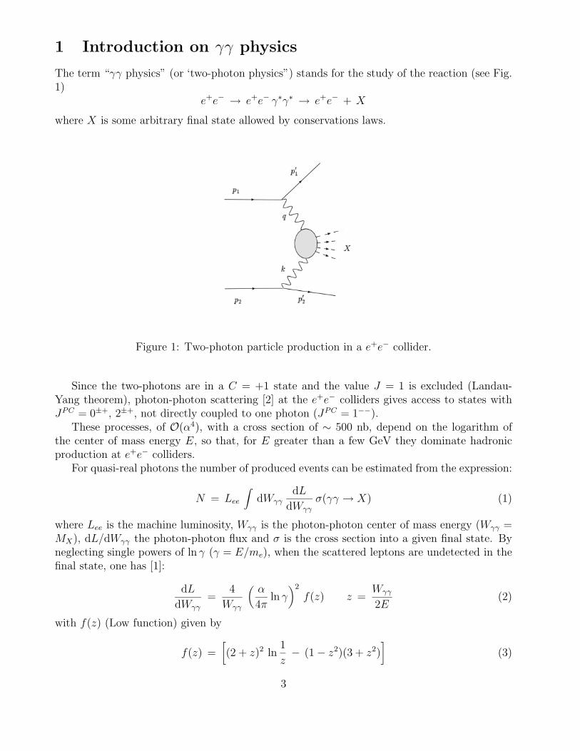
The term “γγ physics” (or ‘two-photon physics”) stands for the study of the reaction (see Fig.1)

e+e− → e+e− γ∗γ∗ → e+e− + X

where X is some arbitrary final state allowed by conservations laws.

Figure 1: Two-photon particle production in a e+e− collider.

Since the two-photons are in a C = +1 state and the value J = 1 is excluded (Landau-Yang theorem), photon-photon scattering [2] at the e+e− colliders gives access to states withJPC = 0±+, 2±+, not directly coupled to one photon (JPC = 1−−).

These processes, of O(α4), with a cross section of ∼ 500 nb, depend on the logarithm ofthe center of mass energy E, so that, for E greater than a few GeV they dominate hadronicproduction at e+e− colliders.

For quasi-real photons the number of produced events can be estimated from the expression:

N = Lee

∫dWγγ

dL

dWγγ

σ(γγ → X) (1)

where Lee is the machine luminosity, Wγγ is the photon-photon center of mass energy (Wγγ =MX), dL/dWγγ the photon-photon flux and σ is the cross section into a given final state. Byneglecting single powers of ln γ (γ = E/me), when the scattered leptons are undetected in thefinal state, one has [1]:

dL

dWγγ

=4

Wγγ

(α

4πln γ

)2

f(z) z =Wγγ

2E(2)

with f(z) (Low function) given by

f(z) =[(2 + z)2 ln

1

z− (1− z2)(3 + z2)

](3)

3

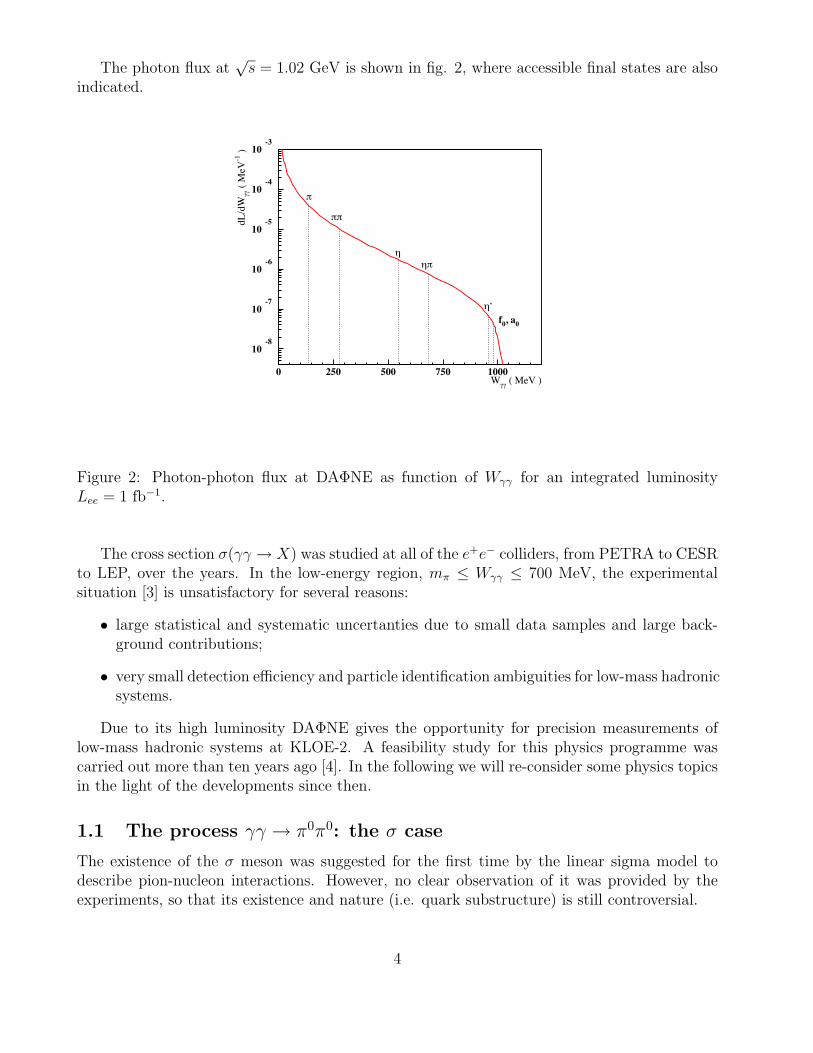
The photon flux at√s = 1.02 GeV is shown in fig. 2, where accessible final states are also

indicated.

!

!!

""!

",

f0, a0

W## ( MeV )

dL/d

W##

( M

eV-1

)

10-8

10-7

10-6

10-5

10-4

10-3

0 250 500 750 1000

Figure 2: Photon-photon flux at DAΦNE as function of Wγγ for an integrated luminosityLee = 1 fb−1.

The cross section σ(γγ → X) was studied at all of the e+e− colliders, from PETRA to CESRto LEP, over the years. In the low-energy region, mπ ≤ Wγγ ≤ 700 MeV, the experimentalsituation [3] is unsatisfactory for several reasons:

• large statistical and systematic uncertanties due to small data samples and large back-ground contributions;

• very small detection efficiency and particle identification ambiguities for low-mass hadronicsystems.

Due to its high luminosity DAΦNE gives the opportunity for precision measurements oflow-mass hadronic systems at KLOE-2. A feasibility study for this physics programme wascarried out more than ten years ago [4]. In the following we will re-consider some physics topicsin the light of the developments since then.

1.1 The process γγ → π0π0: the σ case

The existence of the σ meson was suggested for the first time by the linear sigma model todescribe pion-nucleon interactions. However, no clear observation of it was provided by theexperiments, so that its existence and nature (i.e. quark substructure) is still controversial.

4

Recently, the situation has changed. It has been shown [5] that the ππ scattering amplitudecontains a pole with the quantum numbers of vacuum with a mass of Mσ = 441+16

−8 MeV and awidth Γσ = 544+25

−18 MeV. The σ has been looked for also in D decays by the E791 Collaborationat Fermilab [6]. From the D → 3π Dalitz plot analysis, E791 finds that almost 46% of thewidth is due to D → σπ with Mσ = 478± 23± 17 MeV and Γσ = 324± 40± 21 MeV. BES [7]has looked for the σ in J/ψ → ωπ+π− giving a mass value of Mσ = 541± 39 MeV and a widthof Γσ = 252± 42 MeV.

It is worth to notice that the interest in assessing the existence and nature of the σ mesonis not confined to low energy phenomenology. Just to mention a possible relevant physicalscenario in which the σ could play a role, consider the contamination of B → σπ in B → ρπdecays (possible because of the large σ width). This could affect the isospin analysis for theCKM-α angle extraction [8]. Similarly studies of the γ angle through a Dalitz analysis of neutralD decays need the presence of a σ resonance [9].

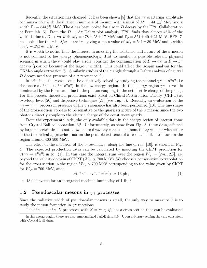
In principle, the σ case could be definitively solved by studying the channel γγ → π0π0 (i.ethe process e+e− → e+e−π0π0), in the low energy region. (In this energy region γγ → ππ− isdominated by the Born term due to the photon coupling to the net electric charge of the pions).For this process theoretical predictions exist based on Chiral Perturbation Theory (CHPT) attwo-loop level [20] and dispersive techniques [21] (see Fig. 3). Recently, an evaluation of theγγ → π0π0 process in presence of the σ resonance has also been performed [10]. The line shapeof the cross-section appears to be sensitive to the quark structure of the σ meson, since the twophotons directly couple to the electric charge of the constituent quarks.

From the experimental side, the only avalaible data in the energy region of interest comefrom Crystal Ball collaboration [3]1. Unfortunately, as show from Fig. 3, these data, affectedby large uncertainties, do not allow one to draw any conclusion about the agreement with eitherof the theoretical approaches, nor on the possible existence of a resonance-like structure in theregion around 400-500 MeV.

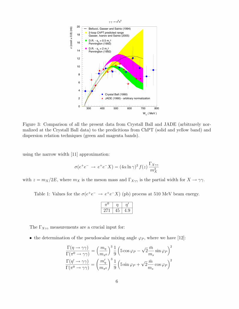
The effect of the inclusion of the σ resonance, along the line of ref. [10], is shown in Fig.4. The expected production rates can be calculated by inserting the ChPT prediction forσ(γγ → π0π0) in eq. (1). In this case the integral runs over the region Wγγ = [2mπ, 2E], i.e.beyond the validity domain of ChPT (Wγγ ≤ 700 MeV). We choose a conservative extrapolationfor the cross section in the region Wγγ > 700 MeV corresponding to the value given by ChPTfor Wγγ = 700 MeV, and:

σ(e+e− → e+e− π0π0) ' 13 pb , (4)

i.e. 13,000 events for an integrated machine luminosity of 1 fb−1.

1.2 Pseudoscalar mesons in γγ processes

Since the radiative width of pseudoscalar mesons is small, the only way to measure it is tostudy the meson formation in γγ reactions.

The e+e− → e+e−X processes, with X = π0, η, η′, has a cross section that can be evaluated

1In this energy region there are also unnormalized JADE data [19]. Upon arbitrary scaling they are consistentwith Crystal Ball data.

5

0

2

4

6

8

10

12

14

16

18

20

300 400 500 600 700 800

JADE (1990) - arbitrary normalizationCrystal Ball (1990)

2-loop ChPT predicted rangeGasser, Ivanov and Sainio (2005)

Bellucci, Gasser and Sainio (1994)

D.R. - sn = 0.5 m!2

Pennington (1992)

D.R. - sn = 2 m!2

Pennington (1992)

" " # !0!0

W"" ( MeV )

$ (c

os% &

0.8)

(nb)

Figure 3: Comparison of all the present data from Crystall Ball and JADE (arbitrarely nor-malized at the Crystall Ball data) to the predicitions from ChPT (solid and yellow band) anddispersion relation techniques (green and magenta bands).

using the narrow width [11] approximation:

σ(e+e− → e+e−X) = (4α ln γ)2 f(z)ΓXγγm3X

with z = mX/2E, where mX is the meson mass and ΓXγγ is the partial width for X → γγ.

Table 1: Values for the σ(e+e− → e+e−X) (pb) process at 510 MeV beam energy.

π0 η η′

271 45 4.9

The ΓXγγ measurements are a crucial input for:

• the determination of the pseudoscalar mixing angle ϕP , where we have [12]:

Γ(η → γγ)

Γ(π0 → γγ)=(mη

mπ0

)3 1

9

(5 cosϕP −

√2m

ms

sinϕP

)2

Γ(η′ → γγ)

Γ(π0 → γγ)=

(m′ηmπ0

)31

9

(5 sinϕP +

√2m

ms

cosϕP

)2

6

300 400 500 600 700 800WΓΓ�MeV�0

2

4

6

8

10

12

14

Σ�nb�

Figure 4: The Crystall Ball data and the two-loop ChPT prediction (red curve) of Fig. 3 arecompared with the the cross section for the process γγ → σ → π0π0 calculated in ref. [10] (blucurve).

• the test for valence gluon content in the η′ wavefunction [13, 14]:

Γ(η′ → γγ)

Γ(π0 → γγ)=

(m′ηmπ0

)31

9cos2 φG

(5 sinϕP +

√2fnfs

cosϕP

)2

Furthermore, a precise study of the form factors [15] of the transition γγ∗ → X, F (Q2γ∗ , 0) =

F (Q2γ∗), where one photon is off-shell and the other is real, allows one to test:

• phenomenological models used for computing the light-by-light contributions to the (gµ−2)/2 prediction in the Standard Model [16];

• the dynamics of the π0 → e+e− transition [18], whose branching fraction value wasrecently measured by the KTeV experiment [17] and is apparently larger than the unitaritybound derived from π0 → γγ.

7

2 Experimental considerations

In the following we will focus our attention on the measurement of γγ → π0π0. To improveon the measurement of the γγ → π0π0 cross section, high statistics has to be complementedby a careful control of the systematics which cannot be obtained without strong reduction ofbackground events. The main source of background comes from φ decays. Studies currentlyunderway on the KLOE data sample are using the off-peak data in order to evaluate theexperimental capabilities leaving aside most of the background from φ decays. At KLOE-2 weaim to analyze the on-peak sample performing background suppression with the informationcoming from a tagger system for efficient detection of scattered electrons. Then, on the taggedsample, we can use the kinematical constraint on the total transverse momentum (pT ) of theparticles in KLOE to further suppress the events from e+e− annihilation, that have higherpT with respect to γγ ones. It is worthwhile to mention that tagging the two-photon eventswould also be useful to reject a possible background for particular measurements of one-photonprocesses, like the measurement of the e+e− → π+π− cross section from Initial State Radiationevents.

From the study of the kinematics of the reaction e+e− → e+e−ππ the most of the scatteredelectrons are emitted in the forward directions, escaping detection. Since the energy of theseelectrons is less than 510 MeV, they deviate from the equilibrium orbit during their propagationalong the machine lattice. Therefore a tagging system should consists of one or more detectorslocated in well identified regions along the beam line, aimed at determining the energy of thescattered electrons either directly, or from the measurement of their displacement from themain orbit.

To fix the characteristics of the tagging detectors and their location along the machine layoutwe made a complete study of the tracking of the final leptons in the process e+e− → e+e−π0π0

along the machine optics.

2.1 Tracking of the off-energy leptons in the machine lattice

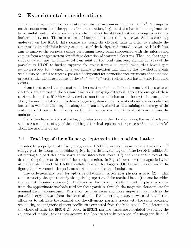
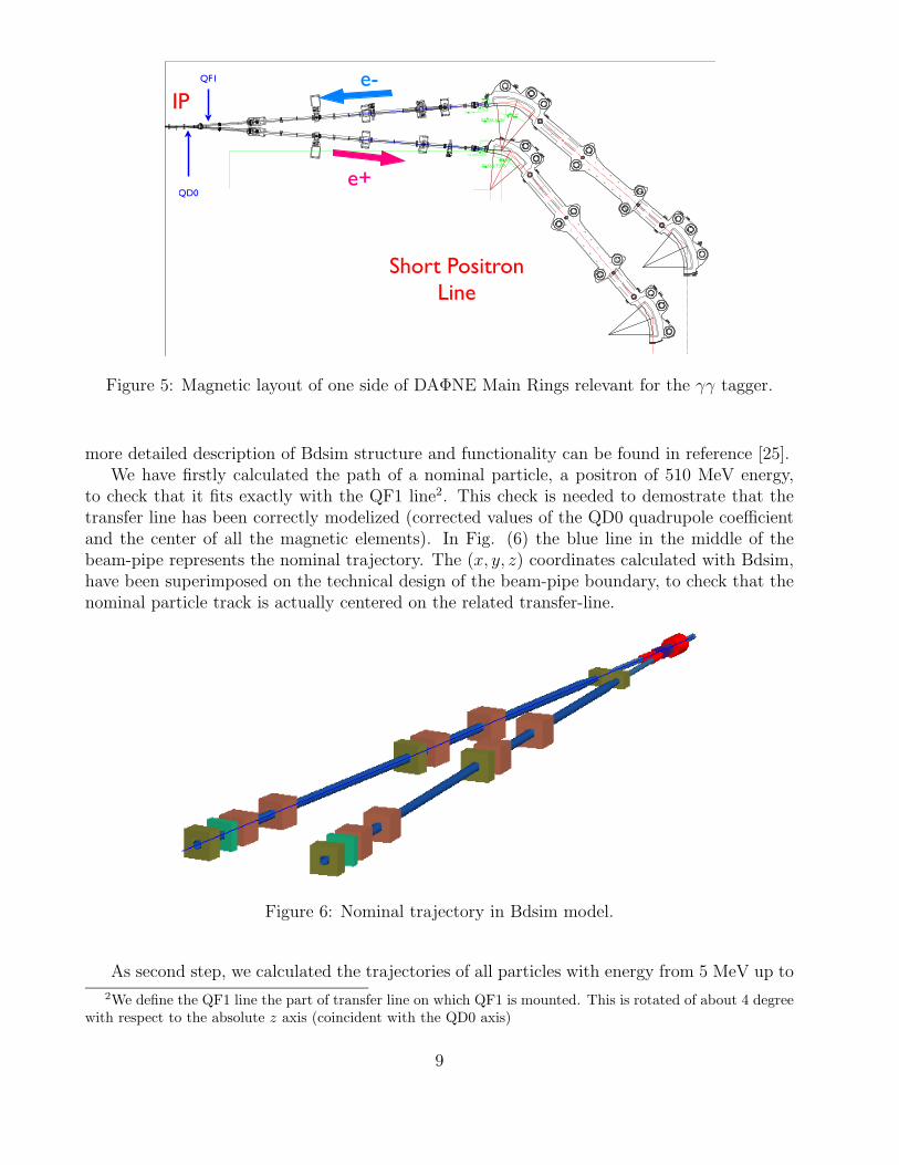
In order to properly locate the γγ taggers in DAΦNE, we need to accurately track the off-energy particles along the machine optics. In particular, the region of the DAΦNE collider forestimating the particles path starts at the interaction Point (IP) and ends at the exit of thefirst bending dipole at the end of the straight section. In Fig. (5) we show the magnetic layoutof the transfer line of the DAΦNE collider relevant for taggers. Of the two lines shown in thefigure, the lower one is the positron short line, used for the simulations.

The code generally used for optics calculations in accelerator physics is Mad [23]. Thiscode is strictly thought to study the optical properties of the nominal beam (the one for whichthe magnetic elements are set). The error in the tracking of off-momentum particles comesfrom the approximate methods used for these particles through the magnetic elements, set fornominal design momentum. This error becomes more and more important as much as theparticle energy deviate from the nominal one. For our study, however, we need a tool thatallows us to calculate the nominal and the off-energy particle tracks with the same precision,while using the magnetic element coefficients extracted from the Mad model. This determinesthe choice of using the BDSIM [24] code. In BDSIM, particle tracks are calculated by solving theequation of motion, taking into account the Lorentz force in presence of a magnetic field. A

8

IP

QD0

QF1

e+

e-

Short Positron

Line

Figure 5: Magnetic layout of one side of DAΦNE Main Rings relevant for the γγ tagger.

more detailed description of Bdsim structure and functionality can be found in reference [25].We have firstly calculated the path of a nominal particle, a positron of 510 MeV energy,

to check that it fits exactly with the QF1 line2. This check is needed to demostrate that thetransfer line has been correctly modelized (corrected values of the QD0 quadrupole coefficientand the center of all the magnetic elements). In Fig. (6) the blue line in the middle of thebeam-pipe represents the nominal trajectory. The (x, y, z) coordinates calculated with Bdsim,have been superimposed on the technical design of the beam-pipe boundary, to check that thenominal particle track is actually centered on the related transfer-line.

Figure 6: Nominal trajectory in Bdsim model.

As second step, we calculated the trajectories of all particles with energy from 5 MeV up to

2We define the QF1 line the part of transfer line on which QF1 is mounted. This is rotated of about 4 degreewith respect to the absolute z axis (coincident with the QD0 axis)

9

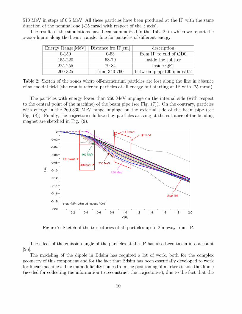
510 MeV in steps of 0.5 MeV. All these particles have been produced at the IP with the samedirection of the nominal one (-25 mrad with respect of the z axis).

The results of the simulations have been summarized in the Tab. 2, in which we report thez-coordinate along the beam transfer line for particles of different energy.

Energy Range[MeV] Distance fro IP[cm] description0-150 0-53 from IP to end of QD0

155-220 53-79 inside the splitter225-255 79-84 inside QF1260-325 from 340-760 between quaps100-quaps102

Table 2: Sketch of the zones where off-momentum particles are lost along the line in absenceof solenoidal field (the results refer to particles of all energy but starting at IP with -25 mrad).

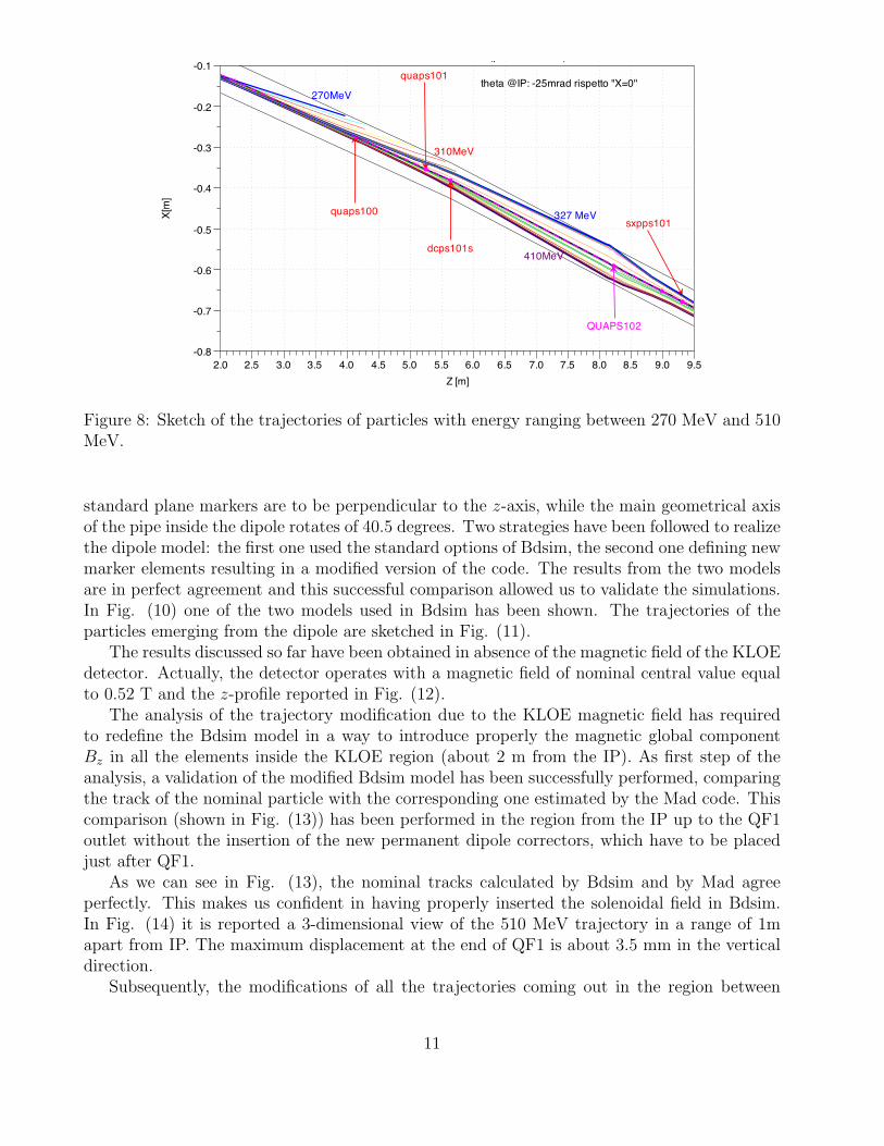
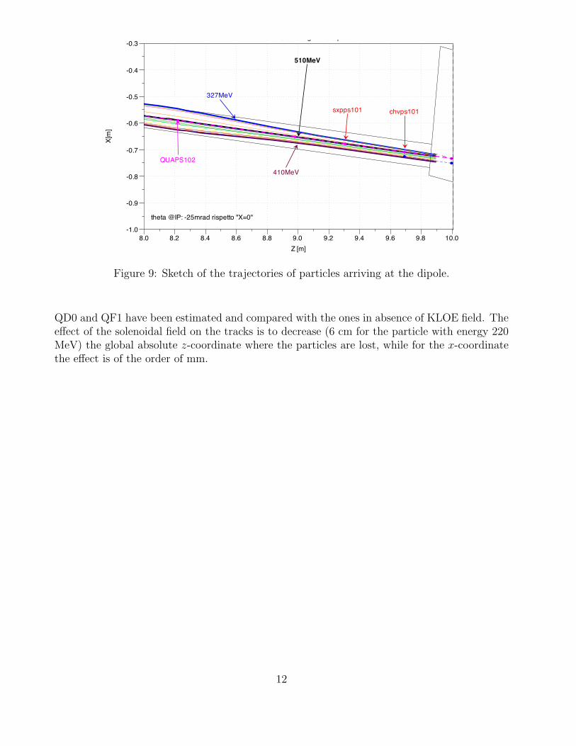
The particles with energy lower than 260 MeV impinge on the internal side (with respectto the central point of the machine) of the beam pipe (see Fig. (7)). On the contrary, particleswith energy in the 260-330 MeV range impinge on the external side of the beam-pipe (seeFig. (8)). Finally, the trajectories followed by particles arriving at the entrance of the bendingmagnet are sketched in Fig. (9).

160 MeV

230 MeV

QF1startQF1end

QD0start

QD0end

270 MeV

theta @IP: -25mrad rispetto "X=0"

chvpi101

X[m

]

-0.20

-0.18

-0.16

-0.14

-0.12

-0.10

-0.08

-0.06

-0.04

-0.02

0

Z [m]

0.2 0.4 0.6 0.8 1.0 1.2 1.4 1.6 1.8 2.0

Particle tracks for Global Z in [0;2m]

Figure 7: Sketch of the trajectories of all particles up to 2m away from IP.

The effect of the emission angle of the particles at the IP has also been taken into account[26].

The modeling of the dipole in Bdsim has required a lot of work, both for the complexgeometry of this component and for the fact that Bdsim has been essentially developed to workfor linear machines. The main difficulty comes from the positioning of markers inside the dipole(needed for collecting the information to reconstruct the trajectories), due to the fact that the

10

theta @IP: -25mrad rispetto "X=0"

dcps101s

quaps100

quaps101

sxpps101

QUAPS102

327 MeV

270MeV

310MeV

410MeV

X[m

]

-0.8

-0.7

-0.6

-0.5

-0.4

-0.3

-0.2

-0.1

Z [m]

2.0 2.5 3.0 3.5 4.0 4.5 5.0 5.5 6.0 6.5 7.0 7.5 8.0 8.5 9.0 9.5

Traiettorie da 270 a 510 MeV (passo 10 MeV )

Figure 8: Sketch of the trajectories of particles with energy ranging between 270 MeV and 510MeV.

standard plane markers are to be perpendicular to the z-axis, while the main geometrical axisof the pipe inside the dipole rotates of 40.5 degrees. Two strategies have been followed to realizethe dipole model: the first one used the standard options of Bdsim, the second one defining newmarker elements resulting in a modified version of the code. The results from the two modelsare in perfect agreement and this successful comparison allowed us to validate the simulations.In Fig. (10) one of the two models used in Bdsim has been shown. The trajectories of theparticles emerging from the dipole are sketched in Fig. (11).

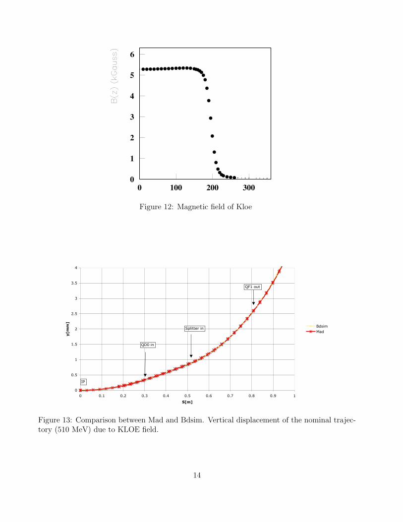
The results discussed so far have been obtained in absence of the magnetic field of the KLOEdetector. Actually, the detector operates with a magnetic field of nominal central value equalto 0.52 T and the z-profile reported in Fig. (12).

The analysis of the trajectory modification due to the KLOE magnetic field has requiredto redefine the Bdsim model in a way to introduce properly the magnetic global componentBz in all the elements inside the KLOE region (about 2 m from the IP). As first step of theanalysis, a validation of the modified Bdsim model has been successfully performed, comparingthe track of the nominal particle with the corresponding one estimated by the Mad code. Thiscomparison (shown in Fig. (13)) has been performed in the region from the IP up to the QF1outlet without the insertion of the new permanent dipole correctors, which have to be placedjust after QF1.

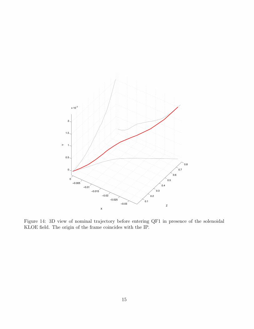
As we can see in Fig. (13), the nominal tracks calculated by Bdsim and by Mad agreeperfectly. This makes us confident in having properly inserted the solenoidal field in Bdsim.In Fig. (14) it is reported a 3-dimensional view of the 510 MeV trajectory in a range of 1mapart from IP. The maximum displacement at the end of QF1 is about 3.5 mm in the verticaldirection.

Subsequently, the modifications of all the trajectories coming out in the region between

11

theta @IP: -25mrad rispetto "X=0"

chvps101 sxpps101

QUAPS102

327MeV

410MeV

510MeV

X[m

]

-1.0

-0.9

-0.8

-0.7

-0.6

-0.5

-0.4

-0.3

Z [m]

8.0 8.2 8.4 8.6 8.8 9.0 9.2 9.4 9.6 9.8 10.0

Particle trcks entering in the dipole

Figure 9: Sketch of the trajectories of particles arriving at the dipole.

QD0 and QF1 have been estimated and compared with the ones in absence of KLOE field. Theeffect of the solenoidal field on the tracks is to decrease (6 cm for the particle with energy 220MeV) the global absolute z-coordinate where the particles are lost, while for the x-coordinatethe effect is of the order of mm.

12

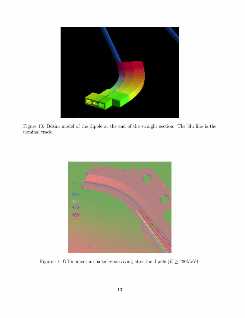
Figure 10: Bdsim model of the dipole at the end of the straight section. The blu line is thenominal track.

Figure 11: Off-momentum particles surviving after the dipole (E ≥ 430MeV).

13

0

1

2

3

4

5

6

0 100 200 300

Figure 12: Magnetic field of Kloe

Confronto Mad-Bdsim (LET region)

0

0.5

1

1.5

2

2.5

3

3.5

4

0 0.1 0.2 0.3 0.4 0.5 0.6 0.7 0.8 0.9 1

S[m]

y[m

m]

Bdsim

Mad

QD0 in

Splitter in

QF1 out

IP

QD0 in

Figure 13: Comparison between Mad and Bdsim. Vertical displacement of the nominal trajec-tory (510 MeV) due to KLOE field.

14

0.1

0.2

0.3

0.4

0.5

0.6

0.7

0.8

!0.03

!0.025

!0.02

!0.015

!0.01

!0.005

0

0

0.5

1

1.5

2

x 10!3

Z

X

Y

Figure 14: 3D view of nominal trajectory before entering QF1 in presence of the solenoidalKLOE field. The origin of the frame coincides with the IP.

15

2.2 The generator for e+e− → e+e−π0π0

We have considered two different generators for the process e+e− → e+e−π0π0:

• The MC code developed by Courau [22] based on the Double Equivalent Photon Approx-imation (DEPA), i.e. the photons emitted by the incoming leptons are considered nearlyon-shell. Therefore, this code cannot properly describe the case in which the final leptonsare emitted at large angles with respect to the incoming ones. On the other hand, it isfast, thus allowing generation of events in any invariant mass range.

• The code developed by Nguyen et al. [10]. Here the σ meson is explicitely inserted as aBreit-Wigner function with mass and width taken from E791 data. This code was tunedfor events generated 20 MeV below the φ resonance peak, i.e. for sqrt(s) = 1 GeV.

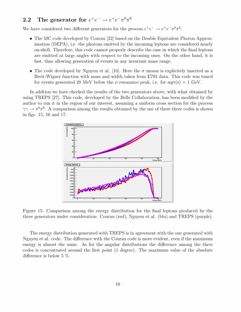
In addtion we have checked the results of the two generators above, with what obtained byusing TREPS [27]. This code, developed by the Belle Collaboration, has been modified by theauthor to run it in the region of our interest, assuming a uniform cross section for the processγγ → π0π0. A comparison among the results obtained by the use of these three codes is shownin figs. 15, 16 and 17.

Energy (MeV)0 0.1 0.2 0.3 0.4 0.5

Per

cen

tag

e(%

)

0

20

40

60

80

100

Cumulative Spectra

Energy (MeV)0 0.1 0.2 0.3 0.4 0.5

No

rmal

ized

En

trie

s

0

0.002

0.004

0.006

0.008

0.01

0.012

0.014

0.016

0.018

0.02

Energy Spectra

Figure 15: Comparison among the energy distribution for the final leptons produced by thethree generators under consideration: Courau (red), Nguyen et al. (blu) and TREPS (purple).

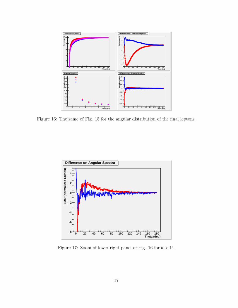
The energy distribution generated with TREPS is in agreement with the one generated withNguyen et al. code. The difference with the Courau code is more evident, even if the maximumenergy is almost the same. As for the angular distributions the difference among the threecodes is concentrated around the first point (1 degree). The maximum value of the absolutedifference is below 5 %.

16

Theta (deg)0 20 40 60 80 100 120 140 160 180

Per

cen

tag

e(%

)

0

20

40

60

80

100

Cumulative Spectra

Theta (deg)0 20 40 60 80 100 120 140 160 180

Per

cen

tag

e(%

)

-8

-6

-4

-2

0

2

Difference on Cumulative Spectra

Theta (deg)0 1 2 3 4 5

No

rmal

ized

En

trie

s

0

0.05

0.1

0.15

0.2

0.25

0.3

0.35

0.4

0.45

Angular Spectra

Theta (deg)0 20 40 60 80 100 120 140 160 180

No

rmal

ized

En

trie

s

-0.04

-0.03

-0.02

-0.01

0

0.01

0.02

0.03

Difference on Angular Spectra

Figure 16: The same of Fig. 15 for the angular distribution of the final leptons.

Theta (deg)0 20 40 60 80 100 120 140 160 180

1000

*(N

orm

aliz

ed E

ntr

ies)

-8

-6

-4

-2

0

2

4

Difference on Angular Spectra

Figure 17: Zoom of lower-right panel of Fig. 16 for θ > 1o.

17

3 The tagging system

The results of the study described in the previous sections show that, despite the constraintsdue to the DAΦNElayout, a good coverage of the kinematic region of interest can be achieved.Satisfactory results can be obtained by the use of a tagging system composed by two stationslocated at ∼ 1 m and ∼ 11 m from the interaction region, respectively:

• A station to detect leptons at low energy (LET), located in the region between the twoquadrupoles inside KLOE (QD0 and QF1). According to the tracking, the energy of thescattered leptons arriving on this detector is in the interval (160 ÷ 230) MeV.

• A station for leptons with high energy (HET), located at the exit of the first bendingmagnet (about 11 m from the IP). The energy of the scattered particles is in this case(425-490) MeV. The upper limit of the interval is determined by the minimum distance(3 cm) from the main orbit where we can place the detector without interfere with properDAΦNE operations.

Leptons of energy not comprised in the ranges of the LET and the HET can in principle bedetected by a third station (MET) located somewhat in between the other two. This possibilityis however not taken into consideration by the present study, leaving a complete study of theMET for a future note.

3.1 The LET detectors

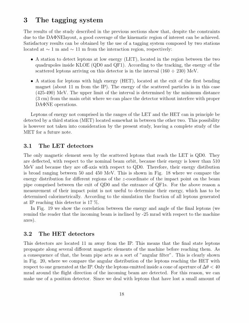
The only magnetic element seen by the scattered leptons that reach the LET is QD0. Theyare deflected, with respect to the nominal beam orbit, because their energy is lower than 510MeV and because they are off-axis with respect to QD0. Therefore, their energy distibutionis broad ranging between 50 and 450 MeV. This is shown in Fig. 18 where we compare theenergy distribution for different regions of the z-coordinate of the impact point on the beampipe comprised between the exit of QD0 and the entrance of QF1s. For the above reason ameasurement of their impact point is not useful to determine their energy, which has to bedetermined calorimetrically. According to the simulation the fraction of all leptons generatedat IP reaching this detector is 17 %.

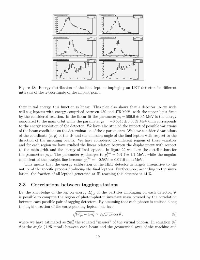
In Fig. 19 we show the correlation between the energy and angle of the final leptons (weremind the reader that the incoming beam is inclined by -25 mrad with respect to the machineaxes).

3.2 The HET detectors

This detectors are located 11 m away from the IP. This means that the final state leptonspropagate along several different magnetic elements of the machine before reaching them. Asa consequence of that, the beam pipe acts as a sort of ”angular filter”. This is clearly shownin Fig. 20, where we compare the angular distribution of the leptons reaching the HET withrespect to one generated at the IP. Only the leptons emitted inside a cone of aperture of ∆θ < 40mrad around the flight direction of the incoming beam are detected. For this reason, we canmake use of a position detector. Since we deal with leptons that have lost a small amount of

18

Energy (MeV)0 100 200 300 400 5000

50

100

150

200

250

300

350

400

Energia{Zend>=0.50&&Zend<0.55} Energia_0Entries 15338Mean 221.2RMS 100.2

Energia{Zend>=0.50&&Zend<0.55}

Energy (MeV)0 100 200 300 400 5000

20

40

60

80

100

120

140

160

180

Energia{Zend>=0.55&&Zend<0.60} Energia_1Entries 4471Mean 205.5RMS 72.61

Energia{Zend>=0.55&&Zend<0.60}

Energy (MeV)0 100 200 300 400 5000

20

40

60

80

100

120

Energia{Zend>=0.60&&Zend<0.65} Energia_2

Entries 3127Mean 220.8RMS 73.93

Energia{Zend>=0.60&&Zend<0.65}

Energy (MeV)0 100 200 300 400 5000

10

20

30

40

50

60

70

Energia{Zend>=0.65&&Zend<0.70} Energia_3

Entries 1476Mean 204RMS 65.55

Energia{Zend>=0.65&&Zend<0.70}

Energy (MeV)0 100 200 300 400 5000

10

20

30

40

50

60

Energia{Zend>=0.70&&Zend<0.75} Energia_4Entries 3114Mean 289.5RMS 113.4

Energia{Zend>=0.70&&Zend<0.75}

Energy (MeV)0 100 200 300 400 5000

20

40

60

80

100

120

Energia{Zend>=0.75&&Zend<0.80} Energia_5Entries 5813Mean 312.5RMS 100.7

Energia{Zend>=0.75&&Zend<0.80}

Figure 18: Energy distribution of the final leptons impinging on LET detector for differentintervals of the z-coordinate of the impact point.

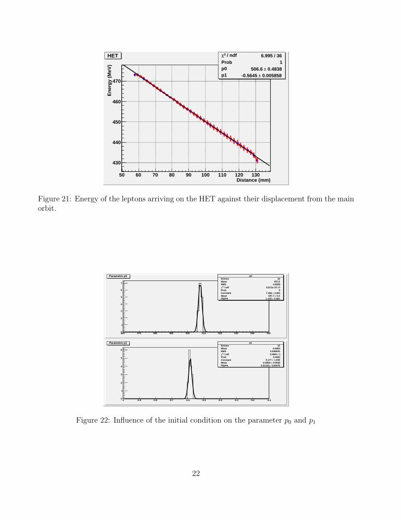
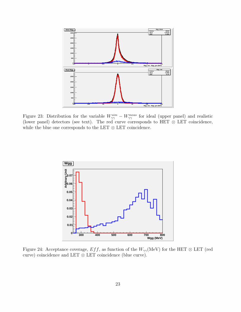
their initial energy, this function is linear. This plot also shows that a detector 15 cm widewill tag leptons with energy comprised between 430 and 475 MeV, with the upper limit fixedby the considered reaction. In the linear fit the parameter p0 = 506.6± 0.5 MeV is the energyassociated to the main orbit while the parameter p1 = −0.5645±0.0059 MeV/mm correspondsto the energy resolution of the detector. We have also studied the impact of possible variationsof the beam conditions on the determination of these parameters. We have considered variationsof the coordinate (x, y) of the IP and the emission angle of the final lepton with respect to thedirection of the incoming beams. We have considered 15 different regions of these variablesand for each region we have studied the linear relation between the displacement with respectto the main orbit and the energy of final leptons. In figure 22 we show the distributions forthe parameters p0,1. The parameter p0 changes to pfin0 = 507.7 ± 1.1 MeV, while the angular

coefficient of the straight line becomes pfin1 = −0.5854± 0.0110 mm/MeV.This means that the energy calibration of the HET detector is largely insensitive to the

nature of the specific process producing the final leptons. Furthermore, according to the simu-lation, the fraction of all leptons generated at IP reaching this detector is 14 %.

3.3 Correlations between tagging stations

By the knowledge of the lepton energy E ′1,2 of the particles impinging on each detector, itis possible to compute the region of photon-photon invariant mass covered by the correlationbetween each possible pair of tagging detectors. By assuming that each photon is emitted alongthe flight direction of the corresponding lepton, one has:√

W 2γγ − 4m2

e ' 2√ω1ω2 cos θ , (5)

where we have estimated as 2m2e the squared ”masses” of the virtual photon. In equation (5)

θ is the angle (±25 mrad) between each beam and the geometrical axes of the machine and

19

Energy (MeV)0 100 200 300 400 500

Th

eta

(rad

)

-0.05

-0.045

-0.04

-0.035

-0.03

-0.025

-0.02

-0.015

-0.01

-0.005

0

Energia:Theta{Zend>=0.50&&Zend<0.55} Energia_Theta_0Entries 15338Mean x 221.9Mean y -0.03247RMS x 98.88RMS y 0.007592

Energia:Theta{Zend>=0.50&&Zend<0.55}

Energy (MeV)0 100 200 300 400 500

Th

eta

(rad

)

-0.05

-0.045

-0.04

-0.035

-0.03

-0.025

-0.02

-0.015

-0.01

-0.005

0

Energia:Theta{Zend>=0.55&&Zend<0.60} Energia_Theta_1Entries 4471Mean x 207.6Mean y -0.02811RMS x 70.7RMS y 0.006199

Energia:Theta{Zend>=0.55&&Zend<0.60}

Energy (MeV)0 100 200 300 400 500

Th

eta

(rad

)

-0.05

-0.045

-0.04

-0.035

-0.03

-0.025

-0.02

-0.015

-0.01

-0.005

0

Energia:Theta{Zend>=0.60&&Zend<0.65} Energia_Theta_2

Entries 3127Mean x 222.9Mean y -0.02804RMS x 72.06RMS y 0.006376

Energia:Theta{Zend>=0.60&&Zend<0.65}

Energy (MeV)0 100 200 300 400 500

Th

eta

(rad

)

-0.05

-0.045

-0.04

-0.035

-0.03

-0.025

-0.02

-0.015

-0.01

-0.005

0

Energia:Theta{Zend>=0.65&&Zend<0.70} Energia_Theta_3

Entries 1476Mean x 209.2Mean y -0.02677RMS x 60.82RMS y 0.005936

Energia:Theta{Zend>=0.65&&Zend<0.70}

Energy (MeV)0 100 200 300 400 500

Th

eta

(rad

)

-0.05

-0.045

-0.04

-0.035

-0.03

-0.025

-0.02

-0.015

-0.01

-0.005

0

Energia:Theta{Zend>=0.70&&Zend<0.75} Energia_Theta_4Entries 3114Mean x 273.7Mean y -0.02316RMS x 110RMS y 0.009698

Energia:Theta{Zend>=0.70&&Zend<0.75}

Energy (MeV)0 100 200 300 400 500

Th

eta

(rad

)

-0.05

-0.045

-0.04

-0.035

-0.03

-0.025

-0.02

-0.015

-0.01

-0.005

0

Energia:Theta{Zend>=0.75&&Zend<0.80} Energia_Theta_5Entries 5813Mean x 306.9Mean y -0.02138RMS x 99.54RMS y 0.01035

Energia:Theta{Zend>=0.75&&Zend<0.80}

Figure 19: Angle vs Energy correlation of the leptons impinging on LET detector. The intervalsof z-coordinate of the impact point are the same of Fig. 18.

ω1,2 = E − E ′1,2 are the energies of the two photons, respectively. More generally, the photonsare emitted at angle with respect to the leptons flight direction. This translates in an effectiveθ to be inserted in equation (5). This angle can be evaluted by using the Courau generator,and turns out 〈θ〉 = 69.5 ± 51.7 mrad. Eq. (5) specified for this angle provide us the Wmeas

γγ .By indicating with W sim

γγ the photon-photon invariant mass simulated by the generator, in Fig.23 we show the difference between the W sim

γγ −Wmeasγγ in the ideal case where the HET/LET

detector resolution is infinite, and in a more realistic case where we assume the HET resolution

to be 2pfin1 , i.e. a 2 mm pitch is considered, and LET resolution is σ(E)/E = 5%/√E[Gev].

In the case of the HET ⊗ LET coincidence we have a resolution of σE =8.2 MeV, while in caseof the LET ⊗ LET coincidence we have a resolution of σE = 47 MeV.

In figure 24 the invariant mass coverage for the two coincidence HET ⊗ LET and LET ⊗LET is showed where is clearly indicated that we cover the Wγγ from threshold up to 700 MeV.

3.4 Considerations on backgrounds

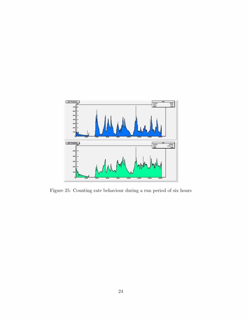
Backgrounds, generated by Touschek effect or radiative Bhabha are a major concern for theproper operation of both HET and LET. We have tried to estimate the amount of the DAΦNEbackground experimentally, during the run of the SIDDHARTA experiment in July 2008. Forthe purpose we have used a prototype of the GRAAL tagging system, consisting of a siliconµstrip 1 mm thick, with 300 µm pitch backed by five 5 × 5 × 6 mm3 Bicron BC418 plasticscintillators located very close the LET position. Another plastic scintillator was located afterthe dipole, close to the HET position but outside the beam pipe which provides a naturalshielding to the detector. In Fig. (25) we report the counting rate of the plastics detectors inthe two location studied during a typical DAΦNE run. The corresponding average luminosity isaround 1032 cm−2s−1. The measured average background is about 200 kHz in the LET locationand 100 kHz in the HET one. These numbers have to intended just as a qualitative estimate

20

Angle (rad)-0.04 -0.02 0 0.02 0.04 0.06

10

210

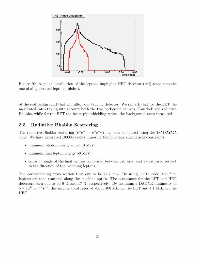
310

410

HET Angle DistibutionHET Angle Distibution

Figure 20: Angular distribution of the leptons impinging HET detector (red) respect to theone of all generated leptons (blalck).

of the real background that will affect our tagging detector. We remark that for the LET themesurated rates taking into account both the two backgroud sources, Touschek and radiativeBhabha, while for the HET the beam pipe shielding reduce the background rates measured.

3.5 Radiative Bhabha Scattering

The radiative Bhabha scattering (e+e− → e+e−γ) has been simulated using the BHABHAYAGA

code. We have generated 100000 events imposing the following kinematical constraints:

• minimum photon energy equal 10 MeV;

• minimun final lepton energy 50 MeV;

• emission angle of the final leptons comprised between 870 µrad and π−870 µrad respectto the direction of the incoming leptons.

The corresponding cross section turn out to be 12.7 mb. By using BDSIM code, the finalleptons are then trackend along the machine optics. The acceptance for the LET and HETdetectors turn out to be 6 % and 17 %, respectively. By assuming a DAΦNE luminosity of5 × 1032 cm−2s−1, this implies total rates of about 400 kHz for the LET and 1.1 MHz for theHET.

21

Distance (mm)50 60 70 80 90 100 110 120 130

En

erg

y (M

eV)

430

440

450

460

470

/ ndf 2χ 6.995 / 36Prob 1p0 0.4838± 506.6 p1 0.005858± -0.5645

/ ndf 2χ 6.995 / 36Prob 1p0 0.4838± 506.6 p1 0.005858± -0.5645

HET

Figure 21: Energy of the leptons arriving on the HET against their displacement from the mainorbit.

p0Entries 15Mean 507.6RMS 0.8369

/ ndf 2χ 9.013e-10 / 0Prob 0Constant 2.651± 7.196 Mean 0.4± 507.7 Sigma 0.487± 1.103

460 470 480 490 500 510 520 530 540 5500

1

2

3

4

5

6

7

p0Entries 15Mean 507.6RMS 0.8369

/ ndf 2χ 9.013e-10 / 0Prob 0Constant 2.651± 7.196 Mean 0.4± 507.7 Sigma 0.487± 1.103

Parametro p0

p1Entries 15Mean -0.5861RMS 0.008045

/ ndf 2χ 0.5801 / 1Prob 0.4463Constant 1.939± 5.177 Mean 0.0040± -0.5854 Sigma 0.00478± 0.01103

-1 -0.9 -0.8 -0.7 -0.6 -0.5 -0.4 -0.3 -0.2 -0.10

1

2

3

4

5

6

p1Entries 15Mean -0.5861RMS 0.008045

/ ndf 2χ 0.5801 / 1Prob 0.4463Constant 1.939± 5.177 Mean 0.0040± -0.5854 Sigma 0.00478± 0.01103

Parametro p1

Figure 22: Influence of the initial condition on the parameter p0 and p1

22

Wgg_mis - Wgg_gen (MeV)-1.5 -1 -0.5 0 0.5 1 1.50

500

1000

1500

2000

2500

3000

Ideal Wgg Wgg_idealeEntries 60000Mean 0.04138RMS 0.1899

Ideal Wgg

Wgg_mis - Wgg_gen (MeV)-150 -100 -50 0 50 100 1500

500

1000

1500

2000

2500

Real Wgg Wgg_realEntries 60000Mean -0.3688RMS 21.22

Real Wgg

Figure 23: Distribution for the variable W simγγ − Wmeas

γγ for ideal (upper panel) and realistic(lower panel) detectors (see text). The red curve corresponds to HET ⊗ LET coincidence,while the blue one corresponds to the LET ⊗ LET coincidence.

Wgg (MeV)300 400 500 600 700 800

Arb

itra

ry U

nit

0

0.01

0.02

0.03

0.04

0.05

0.06

0.07

WggWgg

Figure 24: Acceptance coverage, Eff , as function of the Wγγ(MeV) for the HET ⊗ LET (redcurve) coincidence and LET ⊗ LET coincidence (blue curve).

23

0 2000 4000 6000 8000 10000 12000 14000 160000

100

200

300

400

500

600

700

310×

LET Position tagaEntries 16240Mean 9234RMS 4010

LET Position

0 2000 4000 6000 8000 10000 12000 14000 160000

100

200

300

400

500

310×

HET Position odoEntries 259840Mean 1.001e+04RMS 4035

HET Position

Figure 25: Counting rate behaviour during a run period of six hours

24

4 LET detector design

In the previous chapters the results of the beam simulation were discussed: the knowledge ofexpected direction of the off-energy beam particles allows us to evaluate, as a function of theparticle momentum, where the off-energy electrons and positrons will hit the beam pipe wall.The simulation shows that low energy e+e− , i.e. the ones with energy below 250 MeV, comeout from the beam pipe within one meter from the interaction point. These particles can beidentified by a detector very close to the beam pipe, placed in the horizontal plane. However,off-energy e+e− detectable in this way are only those crossing the beam pipe in a region whereno magnetic element is present, i.e. where it is possible to place a detector. The only freeregion in the zone of interest is the one sitting between the first two quadrupoles close to theIP. There, most of the off-energy e+e− coming out the beam pipe have energy between 160 and230 MeV and an average angle of 11 degrees with respect to the beam axis. The cross sectionof the emitted beam will be 3 cm along the horizontal axis, with negligible vertical spread. Thelatter dimension is mainly due to the effect of the KLOE magnetic field, which is parallel tothe beam axis and deflects off-beam particles in the vertical plane.

The simulation also shows that for these off-energy e+e− there is only a rough correlationbetween particle energy and trajectory, due to the spread of the interaction point and orbit,allowing off-momentum e+e− with energies within few tenth of MeV to pass through the beampipe wall at the same point. This loss of correlation between energy and position makesit necessary to design an energy-sensitive detector, i.e. a calorimeter, instead of a position-sensitive one.

A further costraint to be considered is the presence of the KLOE drift chamber inner wall:this limits the radial dimension of the detector below 20 cm, when accounting also for theclearance necessary to install the inner detectors and the beam pipe.

The inner station of the γγ tagger will therefore consist of a couple of detectors, symmetri-cally placed at both sides of the interaction point, in a position which allows us to detect theescaping beam particles. This inner detector, referred as Low Energy Tagger or LET, consistsof a calorimeter capable of detecting electrons and positrons in the energy range 160-230 MeV.The environmental conditions require radiation-tolerant devices, insensitive to magnetic fields.Concerning the physics requirements, such a detector must allow for high energy and timeresolutions:

• Energy resolution is required to improve the reconstruction of the invariant mass of theγγ decay products, both in case of HET-LET and LET-LET event tagging.

• Time resolution is required to correctely correlate the detected events with the bunchcrossing that has generated them.

• The rate of accidental events due to machine background (Touscheck effect) must also betaken into account. With the new machine design, we expect an accidental event rate of50 MHz, which means 5 MHz of events impinging on the LET detector. A time windowof 5 ns will reduce the accidental rate by a factor 40. Further background rejection willbe obtained by cutting on the deposited energy.

By the above-mentioned requirements we can impose some technological costraints to ourdetector:

25

• It must be made by high-Z material, in order to place a detector with a lenght of severalX0 so to minimize shower leakage,

• If crystals are used, they should have a high light yield, and a fast emission, in order toget the desired timing and energy capabilities,

• Photodetectors must be thin, radiation tolerant, with high gain and insensitive to mag-netic fields.

Several suitable choices are offered by the most recent scintillating crystals and photodetec-tors that can in principle satisfy the above specified requirements. For instance, both the LeadTungstate (PbWO4) and the new Cerium doped Lutetium Yttrium Orthosilicate (LYSO) crys-tal scintillators can be considered, coupled to both Avalanche Photodiodes (APD) and SiliconPhotomultipliers (SiPM) photodetectors.

All these new technological solutions have been investigated and tested in deep, in orderto find the ones best fitting the LET requirements. Details about technical specifications andexperimental tests of these new devices will be discussed in the following.

4.1 Detector simulation

The small available space for the LET, together with financial costraints, makes it neccessaryto carefully choose the dimension of the active part of the detector in order to maximizethe acceptance to e+e− while minimizing the shower leakage. In order to do that, extensiveMonteCarlo simulations, made with the GEANT4 package, have been used to evaluate theexpected energy and time resolution with different geometric options for the final design. A fullsimulation of the LET active volume has been carried out considering both LYSO and PbWO4

crystals; the simulated beam trajectories have been used to exactly determine the detectorresponse to the expected off-momentum particles. By changing detector dimensions and typeof scintillator, we found that the best choice for the dimensions of each of the two LET detectorsis 7.5x6x12 cm3 (x, y, z). Fig. 26 shows the drawings of one of these LET detectors in placealong the beam line. Each detector consists of 20 crystals, pointing to the average direction ofthe off-energy particles, i.e. 11 degrees with respect to the z axis, centered on the horizontalplane. With this design, the energy resolution is 12% for the PbWO4 and 7% for the LYSO.Distributions of the energy deposits for the two options are shown in Fig. 36.

4.2 Experimental considerations

In the following we first discuss the possible options available for the detector choice. We thenshow the test performed with single crystals at electron test beams and summarize the statusfor the realization and test of a complete prototype. We finally recall the status of the testbeam simulation and draw our conclusions on the detector choice.

4.2.1 Technology: crystals and photosensors

The discussion of the previous section indicates that the crystals needed for the Low EnergyTagger (LET) have to be very dense, fast, not igroscopic and with a reasonably high light

26

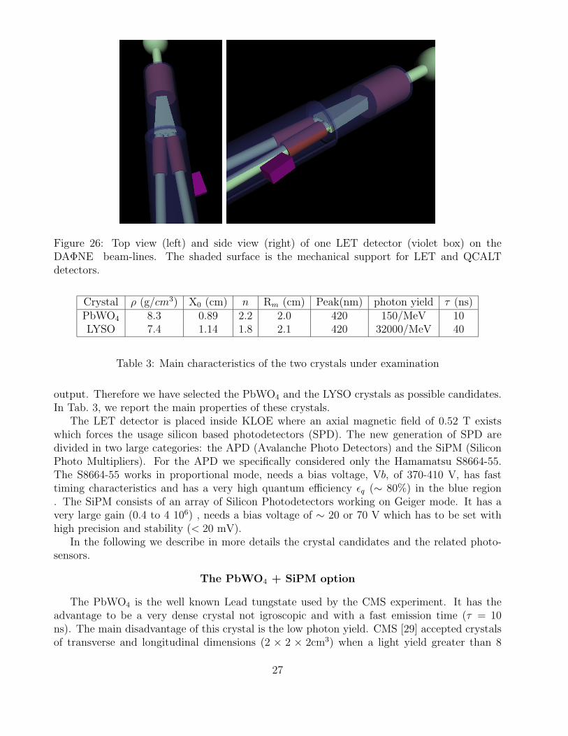
Figure 26: Top view (left) and side view (right) of one LET detector (violet box) on theDAΦNE beam-lines. The shaded surface is the mechanical support for LET and QCALTdetectors.

Crystal ρ (g/cm3) X0 (cm) n Rm (cm) Peak(nm) photon yield τ (ns)PbWO4 8.3 0.89 2.2 2.0 420 150/MeV 10LYSO 7.4 1.14 1.8 2.1 420 32000/MeV 40

Table 3: Main characteristics of the two crystals under examination

output. Therefore we have selected the PbWO4 and the LYSO crystals as possible candidates.In Tab. 3, we report the main properties of these crystals.

The LET detector is placed inside KLOE where an axial magnetic field of 0.52 T existswhich forces the usage silicon based photodetectors (SPD). The new generation of SPD aredivided in two large categories: the APD (Avalanche Photo Detectors) and the SiPM (SiliconPhoto Multipliers). For the APD we specifically considered only the Hamamatsu S8664-55.The S8664-55 works in proportional mode, needs a bias voltage, Vb, of 370-410 V, has fasttiming characteristics and has a very high quantum efficiency εq (∼ 80%) in the blue region. The SiPM consists of an array of Silicon Photodetectors working on Geiger mode. It has avery large gain (0.4 to 4 106) , needs a bias voltage of ∼ 20 or 70 V which has to be set withhigh precision and stability (< 20 mV).

In the following we describe in more details the crystal candidates and the related photo-sensors.

The PbWO4 + SiPM option

The PbWO4 is the well known Lead tungstate used by the CMS experiment. It has theadvantage to be a very dense crystal not igroscopic and with a fast emission time (τ = 10ns). The main disadvantage of this crystal is the low photon yield. CMS [29] accepted crystalsof transverse and longitudinal dimensions (2 × 2 × 2cm3) when a light yield greater than 8

27

Edep/Ein

Eclu/Ein

fit(Eclu/Ein)

f=E/Ein

dN/df

0

200

400

600

800

1000

0.4 0.6 0.8 1 1.2

Edep/EinEclu/Einfit(Eclu/Ein)

f=E/Ein

dN/df

0

250

500

750

1000

1250

0.4 0.6 0.8 1 1.2

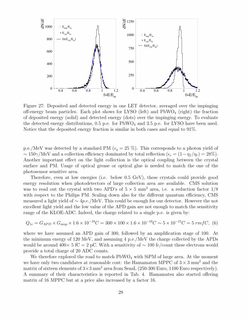
Figure 27: Deposited and detected energy in one LET detector, averaged over the impingingoff-energy beam particles. Each plot shows for LYSO (left) and PbWO4 (right) the fractionof deposited energy (solid) and detected energy (dots) over the impinging energy. To evaluatethe detected energy distributions, 0.5 p.e. for PbWO4 and 3.5 p.e. for LYSO have been used.Notice that the deposited energy fraction is similar in both cases and equal to 91%.

p.e./MeV was detected by a standard PM (εq = 25 %). This corresponds to a photon yield of∼ 150γ/MeV and a collection efficiency dominated by total reflection (εc = (1−ηf/ηr) = 28%).Another important effect on the light collection is the optical coupling between the crystalsurface and PM. Usage of optical grease or optical glue is needed to match the one of thephotosensor sensitive area.

Therefore, even at low energies (i.e. below 0.5 GeV), these crystals could provide goodenergy resolution when photodetectors of large collection area are available. CMS solutionwas to read out the crystal with two APD’s of 5 × 5 mm2 area, i.e. a reduction factor 1/8with respect to the Philips PM. Scaling down also for the different quantum efficiency, CMSmeasured a light yield of ∼ 4p.e./MeV. This could be enough for our detector. However the notexcellent light yield and the low value of the APD gain are not enough to match the sensitivityrange of the KLOE-ADC. Indeed, the charge related to a single p.e. is given by:

Q1e = GAPD×Gamp× 1.6× 10−19C = 300× 100× 1.6× 10−19C ∼ 5× 10−15C = 5 rmfC, (6)

where we have assumed an APD gain of 300, followed by an amplification stage of 100. Atthe minimum energy of 120 MeV, and assuming 4 p.e./MeV the charge collected by the APDswould be around 400× 5 fC = 2 pC. With a sensitivity of ∼ 100 fc/count these electrons wouldprovide a total charge of 20 ADC counts.

We therefore explored the road to match PbWO4 with SiPM of large area. At the momentwe have only two candidates at reasonable cost: the Hamamatsu MPPC of 3× 3 mm2 and thematrix of sixteen elements of 3×3 mm2 area from SensL (250-300 Euro, 1100 Euro respectively).A summary of their characteristics is reported in Tab. 4. Hamamatsu also started offeringmatrix of 16 MPPC but at a price also increased by a factor 16.

28

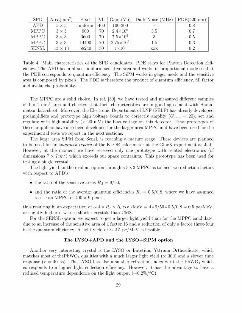
SPD Area(mm2) Pixel Vb Gain (Vb) Dark Noise (MHz) PDE(420 nm)APD 5× 5 uniform 400 100-300 – 0.8

MPPC 3× 3 900 70 2.4×106 3.5 0.7MPPC 3× 3 3600 70 7.5×105 3 0.5MPPC 3× 3 14400 70 2.75×105 1.5 0.3SENSL 13× 13 58240 30 1×106 xxx 0.2

Table 4: Main characteristics of the SPD candidates. PDE stays for Photon Detection Effi-ciency. The APD has a almost uniform sensitive area and works in proportional mode so thatthe PDE corresponds to quantum efficiency. The SiPM works in geiger mode and the sensitivearea is composed by pixels. The PDE is therefore the product of quantum efficiency, fill factorand avalanche probability.

The MPPC are a solid choice. In ref. [30], we have tested and measured different samplesof 1 × 1 mm2 area and checked that their characteristics are in good agreement with Hama-matsu data-sheet. Moreover, the Electronic Department of LNF (SELF) has already developedpreamplifiers and prototype high voltage boards to correctly amplify (Gamp = 20), set andregulate with high stability (< 20 mV) the bias voltage on this detector. First prototypes ofthese amplifiers have also been developed for the larger area MPPC and have been used for theexperimental tests we report in the next sections.

The large area SiPM from SensL is reaching a mature stage. These devices are plannedto be used for an improved replica of the KLOE calorimeter at the GlueX experiment at Jlab.However, at the moment we have received only one prototype with related electronics (ofdimensions 7 × 7cm2) which exceeds our space contraints. This prototype has been used fortesting a single crystal.

The light yield for the readout option through a 3×3 MPPC as to face two reduction factorswith respect to APD’s:

• the ratio of the sensitive areas RA = 9/50,

• and the ratio of the average quantum efficiencies Rε = 0.5/0.8, where we have assumedto use an MPPC of 400× 9 pixels,

thus resulting in an expectation of ∼ 4×RA×Rε p.e./MeV = 4∗9/50∗0.5/0.8 = 0.5 pe/MeV,or slightly higher if we use shorter crystals than CMS.

For the SENSL option, we expect to get a larger light yield than for the MPPC candidate,due to an increase of the sensitive area of a factor 16 and a reduction of only a factor three-fourin the quantum efficiency. A light yield of ∼ 2.5 pe/MeV is feasible.

The LYSO+APD and the LYSO+SiPM option

Another very interesting crystal is the LYSO or Lutetium Yttrium Orthosilicate, whichmatches most of thePbWO4 qualities with a much larger light yield (× 300) and a slower timeresponse (τ = 40 ns). The LYSO has also a smaller refraction index w.r.t the PbWO4 whichcorresponds to a higher light collection efficiency. However, it has the advantage to have areduced temperature dependence on the light output (−0.2%/◦C).

29

0

100

200

300

400

0 250 500 750 1000 1250 1500 1750 2000

E(Adc Counts)

ent

ries

0

100

200

300

0 250 500 750 1000 1250 1500 1750 2000

E(Adc Counts)

ent

ries

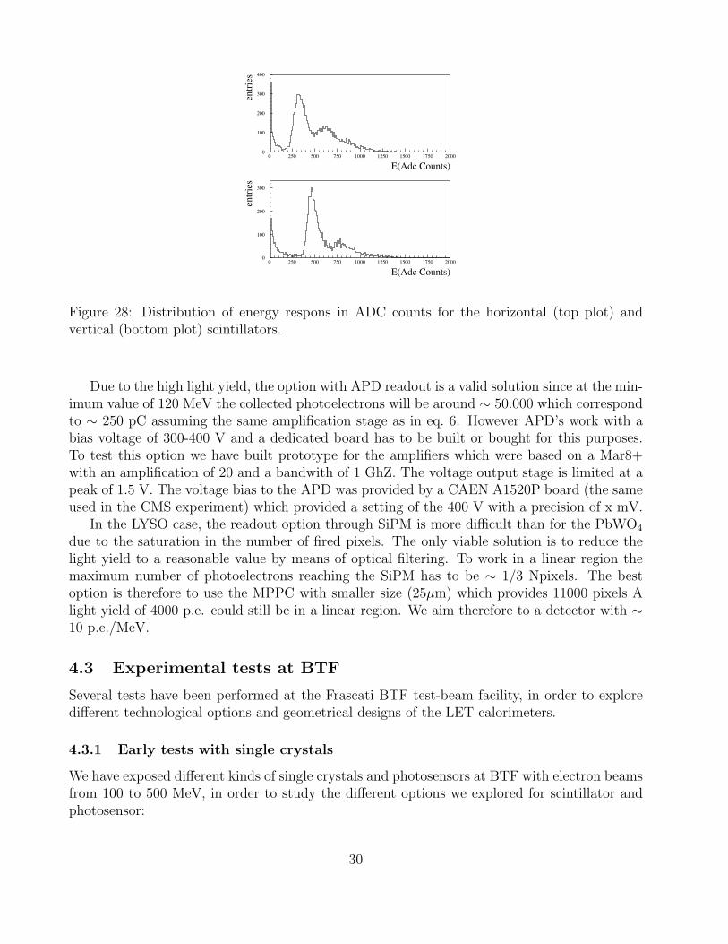
Figure 28: Distribution of energy respons in ADC counts for the horizontal (top plot) andvertical (bottom plot) scintillators.

Due to the high light yield, the option with APD readout is a valid solution since at the min-imum value of 120 MeV the collected photoelectrons will be around ∼ 50.000 which correspondto ∼ 250 pC assuming the same amplification stage as in eq. 6. However APD’s work with abias voltage of 300-400 V and a dedicated board has to be built or bought for this purposes.To test this option we have built prototype for the amplifiers which were based on a Mar8+with an amplification of 20 and a bandwith of 1 GhZ. The voltage output stage is limited at apeak of 1.5 V. The voltage bias to the APD was provided by a CAEN A1520P board (the sameused in the CMS experiment) which provided a setting of the 400 V with a precision of x mV.

In the LYSO case, the readout option through SiPM is more difficult than for the PbWO4

due to the saturation in the number of fired pixels. The only viable solution is to reduce thelight yield to a reasonable value by means of optical filtering. To work in a linear region themaximum number of photoelectrons reaching the SiPM has to be ∼ 1/3 Npixels. The bestoption is therefore to use the MPPC with smaller size (25µm) which provides 11000 pixels Alight yield of 4000 p.e. could still be in a linear region. We aim therefore to a detector with ∼10 p.e./MeV.

4.3 Experimental tests at BTF

Several tests have been performed at the Frascati BTF test-beam facility, in order to exploredifferent technological options and geometrical designs of the LET calorimeters.

4.3.1 Early tests with single crystals

We have exposed different kinds of single crystals and photosensors at BTF with electron beamsfrom 100 to 500 MeV, in order to study the different options we explored for scintillator andphotosensor:

30

0

20

40

60

80

0 5 10 15

Xstrip

entri

es

0

20

40

60

0 5 10 15

Ystrip

entri

es

0

20

40

60

0 2 4 6

Nstrip (x)

entri

es0

25

50

75

100

0 2 4 6

Nstrip (y)

entri

es

Figure 29: Distribution of scintillator strip fired on the X axis (top). Same plot ...

1. C1: a PbWO4 crystal of 2 × 2 × 13 cm3 dimensions wrapped in Tyvek and opticallyconnected by optical grease to a 3600 pixel MPPC. The MPPC was centered in the rearcrystal face by means of a plastic holder.

2. C1bis: a PbWO4 crystal of 1.5×1.5×13 cm3 dimensions readout by a 3600 pixel MPPC.The same crystal have also been tested with a prototype of the SensL photodetector.

3. C2: a LYSO crystal of 2× 2× 13 cm3 dimensions wrapped in Tyvek and with an opticalfilter inserted between the photodetector and the rear face. The filter consisted of differ-ente layers (from 2 to 5) of 100 µm yellow plastic. Another test was done in a identicalconfiguration with a smaller size crystal 2× 2× 10 cm3.

4. C3: 2× 2× 15 cm3 LYSO wrapped in tyvek and optically connected to a 5× 5 o 10× 10mm2 APD.

The crystals were positioned at the center of the beam axis with an area delimited by across of two BC408 scintillators of 1 × 0.5 × 5 cm3 dimensions, f1, f2, just in front of thecrystal face. In most of the tests, the fingers were aligned in such a way that a beam spot of0.5 × 0.5 cm2 was defined. The beam was therefore crossing 2 cm of plastic scintillators (i.e.an average energy loss of ∼ 4 MeV). In front of the fingers a beam position monitor, BPM,was also present; it consisted of sixteen horizontal and vertical scintillator strips readout bytwo Multi Anode PMs. Each strip was built by three 1 mm diameter scintillating fibers thusproviding a sub-mm accuracy on the beam localization.

The trigger and readout scheme were the following:

• we triggered by using a gate synchronized with the beam injection;

• we used either the BTF or the KLOE-2 DAQ systems. In both cases, the trigger gategenerated the ADC & TDC gates. In the KLOE case, we use one standard KLOEcalorimeter ADC and TDC board, the new SDS and the CPU motorola;

31

• the gate was 300 ns long and the sensitivity of the boards was 35 (50) ps/count for theTDC nd 220 (100) fc/count for the ADC boards in the BTF (KLOE) daq.

The BTF beam allows to set the average number of electrons arriving to the detector. Weshow in Fig. 4.2.1, the example of the pulse height seen by one of the fingers. The inclusivedistribution of BPMx, BPMy is also shown in Fig. 4.2.1.

0

2000

4000

6000

0 100 200 300 400 500beam energy (MeV)

AD

C co

unts

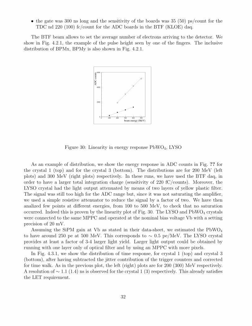
Figure 30: Linearity in energy response PbWO4, LYSO

As an example of distribution, we show the energy response in ADC counts in Fig. ?? forthe crystal 1 (top) and for the crystal 3 (bottom). The distributions are for 200 MeV (leftplots) and 300 MeV (right plots) respectively. In these runs, we have used the BTF daq, inorder to have a larger total integration charge (sensitivity of 220 fC/counts). Moreover, theLYSO crystal had the light output attenuated by means of two layers of yellow plastic filter.The signal was still too high for the ADC range but, since it was not saturating the amplifier,we used a simple resistive attenuator to reduce the signal by a factor of two. We have thenanalized few points at different energies, from 100 to 500 MeV, to check that no saturationoccurred. Indeed this is proven by the linearity plot of Fig. 30. The LYSO and PbWO4 crystalswere connected to the same MPPC and operated at the nominal bias voltage Vb with a settingprecision of 20 mV.

Assuming the SiPM gain at Vb as stated in their data-sheet, we estimated the PbWO4

to have around 250 pe at 500 MeV. This corresponds to ∼ 0.5 pe/MeV. The LYSO crystalprovides at least a factor of 3-4 larger light yield. Larger light output could be obtained byrunning with one layer only of optical filter and by using an MPPC with more pixels.

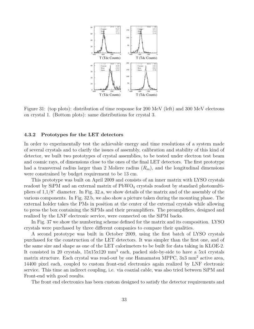
In Fig. 4.3.1, we show the distribution of time response, for crystal 1 (top) and crystal 3(bottom), after having subtracted the jitter contribution of the trigger counters and correctedfor time walk. As in the previous plot, the left (right) plots are for 200 (300) MeV respectively.A resolution of ∼ 1.1 (1.4) ns is observed for the crystal 1 (3) respectively. This already satisfiesthe LET requirement.

32

0

20

40

60

80

-600 -400 -200 0

277.5 / 125Constant 52.47Mean -377.7Sigma 33.35

T (Tdc Counts)0

50

100

150

-600 -400 -200 0

578.0 / 138Constant 125.3Mean -371.8Sigma 31.16

T (Tdc Counts)

0

10

20

30

40

-600 -400 -200 0

216.9 / 127Constant 28.90Mean -224.0Sigma 42.03

T (Tdc Counts)0

50

100

150

200

-600 -400 -200 0

843.6 / 163Constant 118.3Mean -248.2Sigma 37.59

T (Tdc Counts)

Figure 31: (top plots): distribution of time response for 200 MeV (left) and 300 MeV electronson crystal 1. (Bottom plots): same distributions for crystal 3.

4.3.2 Prototypes for the LET detectors

In order to experimentally test the achievable energy and time resolutions of a system madeof several crystals and to clarify the issues of assembly, calibration and stability of this kind ofdetector, we built two prototypes of crystal assemblies, to be tested under electron test beamand cosmic rays, of dimensions close to the ones of the final LET detectors. The first prototypehad a transversal radius larger than 2 Moliere radius (Rm), and the longitudinal dimensionswere constrained by budget requirement to be 13 cm.

This prototype was built on April 2009 and consists of an inner matrix with LYSO crystalsreadout by SiPM and an external matrix of PbWO4 crystals readout by standard photomulti-pliers of 1,1/8” diameter. In Fig. 32.a, we show details of the matrix and of the assembly of thevarious components. In Fig. 32.b, we also show a picture taken during the mounting phase. Theexternal holder takes the PMs in position at the center of the external crystals while allowingto press the box containing the SiPMs and their preamplifiers. The preamplifiers, designed andrealized by the LNF electronic service, were connected on the SiPM backs.

In Fig. 37 we show the numbering scheme defined for the matrix and its composition. LYSOcrystals were purchased by three different companies to compare their qualities.

A second prototype was built in October 2009, using the first batch of LYSO crystalspurchased for the construction of the LET detectors. It was simpler than the first one, and ofthe same size and shape as one of the LET calorimeters to be built for data taking in KLOE-2.It consisted in 20 crystals, 15x15x120 mm3 each, packed side-by-side to have a 5x4 crystalsmatrix structure. Each crystal was read-out by one Hamamatsu MPPC, 3x3 mm2 active area,14400 pixel each, coupled to custom front-end electronics again realized by LNF electronicservice. This time an indirect coupling, i.e. via coaxial cable, was also tried between SiPM andFront-end with good results.

The front end electronics has been custom designed to satisfy the detector requirements and

33

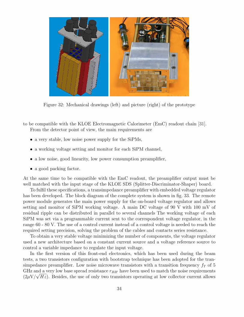
Figure 32: Mechanical drawings (left) and picture (right) of the prototype

to be compatible with the KLOE Electromagnetic Calorimeter (EmC) readout chain [31].From the detector point of view, the main requirements are

• a very stable, low noise power supply for the SiPMs,

• a working voltage setting and monitor for each SiPM channel,

• a low noise, good linearity, low power consumption preamplifier,

• a good packing factor.

At the same time to be compatible with the EmC readout, the preamplifier output must bewell matched with the input stage of the KLOE SDS (Splitter-Discriminator-Shaper) board.

To fulfil these specifications, a transimpedance preamplifier with embedded voltage regulatorhas been developed. The block diagram of the complete system is shown in fig. 33. The remotepower module generates the main power supply for the on-board voltage regulator and allowssetting and monitor of SiPM working voltage. A main DC voltage of 90 V with 100 mV ofresidual ripple can be distributed in parallel to several channels The working voltage of eachSiPM was set via a programmable current sent to the correspondent voltage regulator, in therange 60 - 80 V. The use of a control current instead of a control voltage is needed to reach therequired setting precision, solving the problem of the cables and contacts series resistance.

To obtain a very stable voltage minimizing the number of components, the voltage regulatorused a new architecture based on a constant current source and a voltage reference source tocontrol a variable impedance to regulate the input voltage.

In the first version of this front-end electronics, which has been used during the beamtests, a two transistors configuration with bootstrap technique has been adopted for the tran-simpedance preamplifier. Low noise microwave transistors with a transition frequency fT of 5GHz and a very low base spread resistance rBB′ have been used to match the noise requirements(2µV/

√Hz). Besides, the use of only two transistors operating at low collector current allows

34

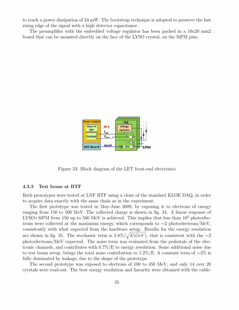
to reach a power dissipation of 24 mW. The bootstrap technique is adopted to preserve the fastrising edge of the signal with a high detector capacitance.

The preamplifier with the embedded voltage regulator has been packed in a 10x20 mm2board that can be mounted directly on the face of the LYSO crystal, on the SiPM pins.

Figure 33: Block diagram of the LET front-end electronics

4.3.3 Test beam at BTF

Both prorotypes were tested at LNF BTF using a clone of the standard KLOE DAQ, in orderto acquire data exactly with the same chain as in the experiment.

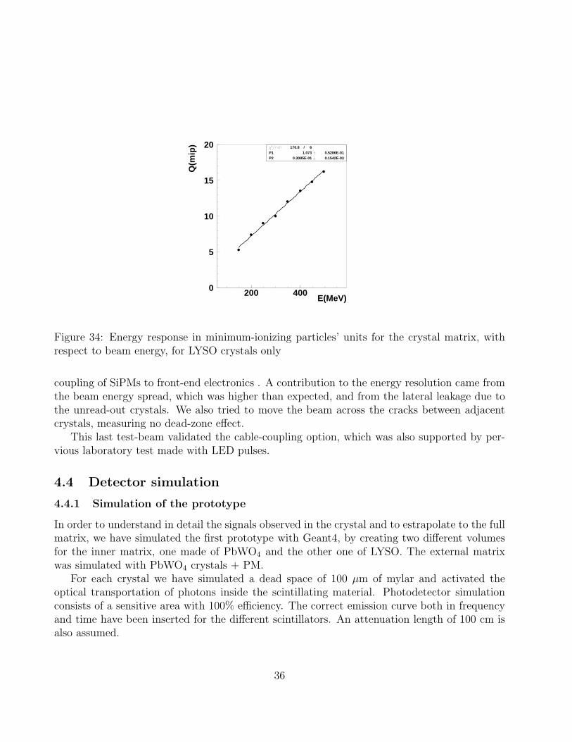
The first prototype was tested in May-June 2009, by exposing it to electrons of energyranging from 150 to 500 MeV. The collected charge is shown in fig. 34. A linear response ofLYSO+SiPM from 150 up to 500 MeV is achieved. This implies that less than 103 photoelec-trons were collected at the maximum energy, which corresponds to ∼2 photoelectrons/MeV,consistently with what expected from the hardware setup. Results for the energy resolution

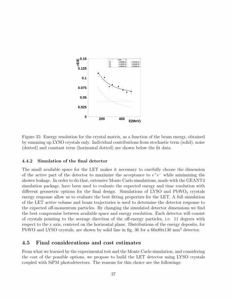
are shown in fig. 35. The stochastic term is 2.8%/√E(GeV ), that is consistent with the ∼2

photoelectrons/MeV expected. The noise term was evaluated from the pedestals of the elec-tronic channels, and contributes with 0.7%/E to energy resolution. Some additional noise dueto test beam setup, brings the total noise contribution to 1.2%/E. A constant term of ∼4% isfully dominated by leakage, due to the shape of the prototype.

The second prototype was exposed to electrons of 100 to 450 MeV, and only 14 over 20crystals were read-out. The best energy resolution and linearity were obtained with the cable-

35

0

5

10

15

20

200 400

170.8 / 6P1 1.073 0.5286E-01P2 0.3085E-01 0.1542E-03

E(MeV)

Q(m

ip)

Figure 34: Energy response in minimum-ionizing particles’ units for the crystal matrix, withrespect to beam energy, for LYSO crystals only

coupling of SiPMs to front-end electronics . A contribution to the energy resolution came fromthe beam energy spread, which was higher than expected, and from the lateral leakage due tothe unread-out crystals. We also tried to move the beam across the cracks between adjacentcrystals, measuring no dead-zone effect.

This last test-beam validated the cable-coupling option, which was also supported by per-vious laboratory test made with LED pulses.

4.4 Detector simulation

4.4.1 Simulation of the prototype

In order to understand in detail the signals observed in the crystal and to estrapolate to the fullmatrix, we have simulated the first prototype with Geant4, by creating two different volumesfor the inner matrix, one made of PbWO4 and the other one of LYSO. The external matrixwas simulated with PbWO4 crystals + PM.

For each crystal we have simulated a dead space of 100 µm of mylar and activated theoptical transportation of photons inside the scintillating material. Photodetector simulationconsists of a sensitive area with 100% efficiency. The correct emission curve both in frequencyand time have been inserted for the different scintillators. An attenuation length of 100 cm isalso assumed.

36

0

0.025

0.05

0.075

0.1

0.125

0.15

200 400

1.634 / 5P1 0.2838E-01 0.1047E-01P2 0.1269E-01 0.6299E-02P3 0.4500E-01 0.3005E-02

E(MeV)

σE/E

Figure 35: Energy resolution for the crystal matrix, as a function of the beam energy, obtainedby summing up LYSO crystals only. Individual contributions from stochastic term (solid), noise(dotted) and constant term (horizontal dotted) are shown below the fit data.

4.4.2 Simulation of the final detector

The small available space for the LET makes it necessary to carefully choose the dimensionof the active part of the detector to maximize the acceptance to e+e− while minimizing theshower leakage. In order to do that, extensive Monte Carlo simulations, made with the GEANT4simulation package, have been used to evaluate the expected energy and time resolution withdifferent geometric options for the final design. Simulations of LYSO and PbWO4 crystalsenergy response allow us to evaluate the best fitting properties for the LET. A full simulationof the LET active volume and beam trajectories is used to determine the detector response tothe expected off-momentum particles. By changing the simulated detector dimensions we findthe best compromise between available space and energy resolution. Each detector will consistof crystals pointing to the average direction of the off-energy particles, i.e. 11 degrees withrespect to the z axis, centered on the horizontal plane. Distributions of the energy deposits, forPbWO and LYSO crystals, are shown by solid line in fig. 36 for a 60x80x130 mm3 detector.

4.5 Final considerations and cost estimates

From what we learned by the experimental test and the Monte Carlo simulation, and consideringthe cost of the possible options, we propose to build the LET detector using LYSO crystalscoupled with SiPM photodetectors. The reasons for this choice are the followings:

37

Edep/EinEclu/Einfit(Eclu/Ein)

f=E/Ein

dN/df

0

250

500

750

1000

1250

0.4 0.6 0.8 1 1.2

Edep/Ein

Eclu/Ein

fit(Eclu/Ein)

f=E/Ein

dN/df

0

200

400

600

800

1000

0.4 0.6 0.8 1 1.2

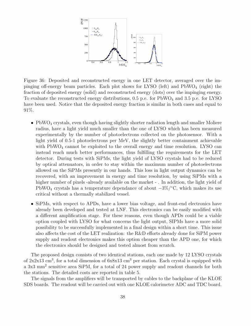
Figure 36: Deposited and reconstructed energy in one LET detector, averaged over the im-pinging off-energy beam particles. Each plot shows for LYSO (left) and PbWO4 (right) thefraction of deposited energy (solid) and reconstructed energy (dots) over the impinging energy.To evaluate the reconstructed energy distributions, 0.5 p.e. for PbWO4 and 3.5 p.e. for LYSOhave been used. Notice that the deposited energy fraction is similar in both cases and equal to91%.

• PbWO4 crystals, even though having slightly shorter radiation length and smaller Moliereradius, have a light yield much smaller than the one of LYSO which has been measuredexperimentally by the number of photoelectrons collected on the photosensor. With alight yield of 0.5-1 photoelectrons per MeV, the slightly better containment achievablewith PbWO4 cannot be exploited to the overall energy and time resolution. LYSO caninstead reach much better performances, thus fulfilling the requirements for the LETdetector. During tests with SiPMs, the light yield of LYSO crystals had to be reducedby optical attenuators, in order to stay within the maximum number of photoelectronsallowed on the SiPMs presently in our hands. This loss in light output dynamics can berecovered, with an improvement in energy and time resolution, by using SiPMs with ahigher number of pixels -already available on the market - . In addition, the light yield ofPbWO4 crystals has a temperature dependance of about −3%/◦C, which makes its usecritical without a thermally stabilized vessel.

• SiPMs, with respect to APDs, have a lower bias voltage, and front-end electronics havealready been developed and tested at LNF. This electronics can be easily modified witha different amplification stage. For these reasons, even though APDs could be a viableoption coupled with LYSO for what concerns the light output, SIPMs have a more solidpossibility to be successfully implemented in a final design within a short time. This issuealso affects the cost of the LET realization: the R&D efforts already done for SiPM powersupply and readout electronics makes this option cheaper than the APD one, for whichthe electronics should be designed and tested almost from scratch.

The proposed design consists of two identical stations, each one made by 12 LYSO crystalsof 2x2x13 cm3, for a total dimension of 6x8x13 cm3 per station. Each crystal is equipped witha 3x3 mm2 sensitive area SiPM, for a total of 24 power supply and readout channels for boththe stations. The detailed costs are reported in table 5.

The signals from the amplifiers will be transported by cables to the backplane of the KLOESDS boards. The readout will be carried out with one KLOE calorimeter ADC and TDC board.

38

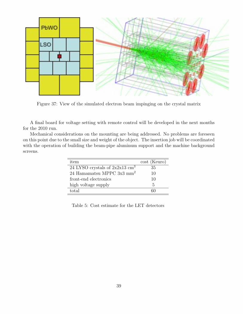
Figure 37: View of the simulated electron beam impinging on the crystal matrix

A final board for voltage setting with remote control will be developed in the next monthsfor the 2010 run.

Mechanical considerations on the mounting are being addressed. No problems are foreseenon this point due to the small size and weight of the object. The insertion job will be coordinatedwith the operation of building the beam-pipe aluminum support and the machine backgroundscreens.

item cost (Keuro)24 LYSO crystals of 2x2x13 cm3 3524 Hamamatsu MPPC 3x3 mm2 10front-end electronics 10high voltage supply 5total 60

Table 5: Cost estimate for the LET detectors

39

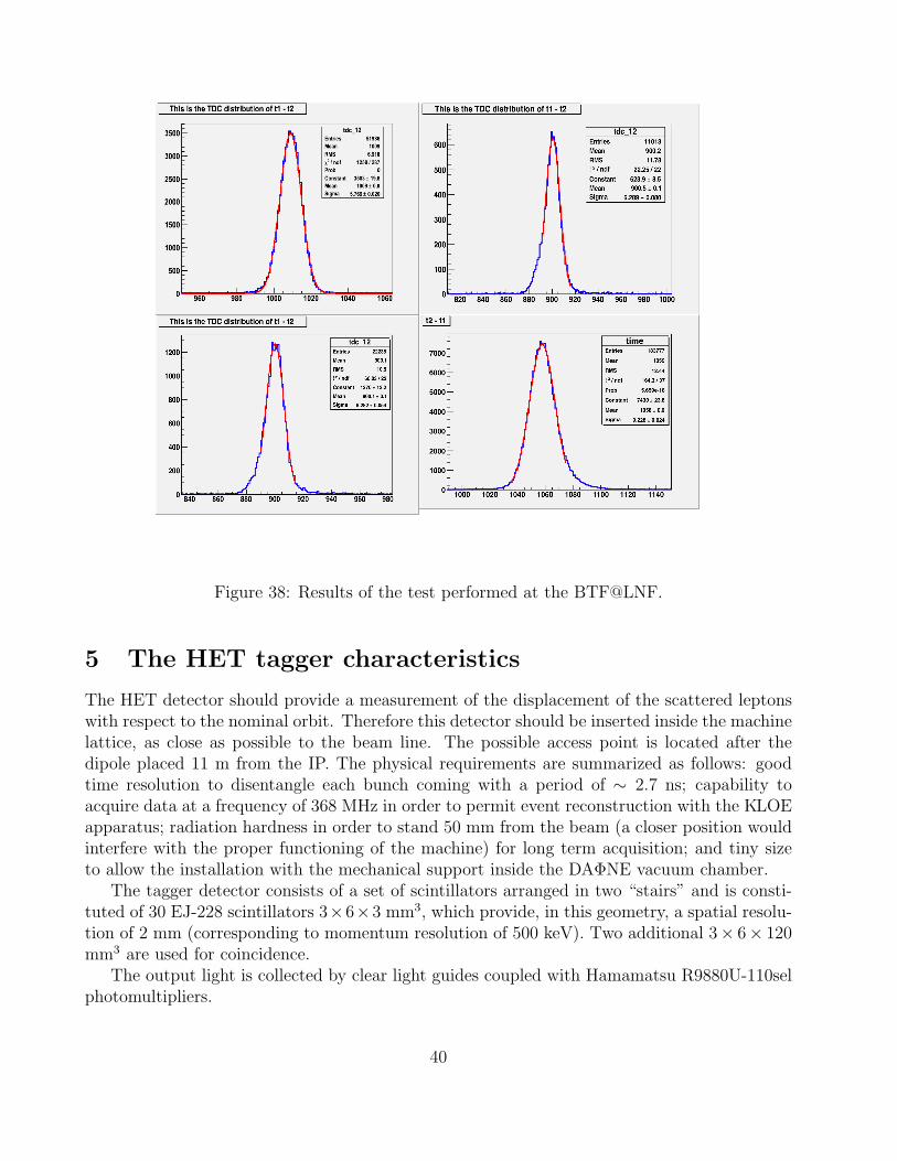
Figure 38: Results of the test performed at the BTF@LNF.

5 The HET tagger characteristics

The HET detector should provide a measurement of the displacement of the scattered leptonswith respect to the nominal orbit. Therefore this detector should be inserted inside the machinelattice, as close as possible to the beam line. The possible access point is located after thedipole placed 11 m from the IP. The physical requirements are summarized as follows: goodtime resolution to disentangle each bunch coming with a period of ∼ 2.7 ns; capability toacquire data at a frequency of 368 MHz in order to permit event reconstruction with the KLOEapparatus; radiation hardness in order to stand 50 mm from the beam (a closer position wouldinterfere with the proper functioning of the machine) for long term acquisition; and tiny sizeto allow the installation with the mechanical support inside the DAΦNE vacuum chamber.

The tagger detector consists of a set of scintillators arranged in two “stairs” and is consti-tuted of 30 EJ-228 scintillators 3×6×3 mm3, which provide, in this geometry, a spatial resolu-tion of 2 mm (corresponding to momentum resolution of 500 keV). Two additional 3× 6× 120mm3 are used for coincidence.

The output light is collected by clear light guides coupled with Hamamatsu R9880U-110selphotomultipliers.

40

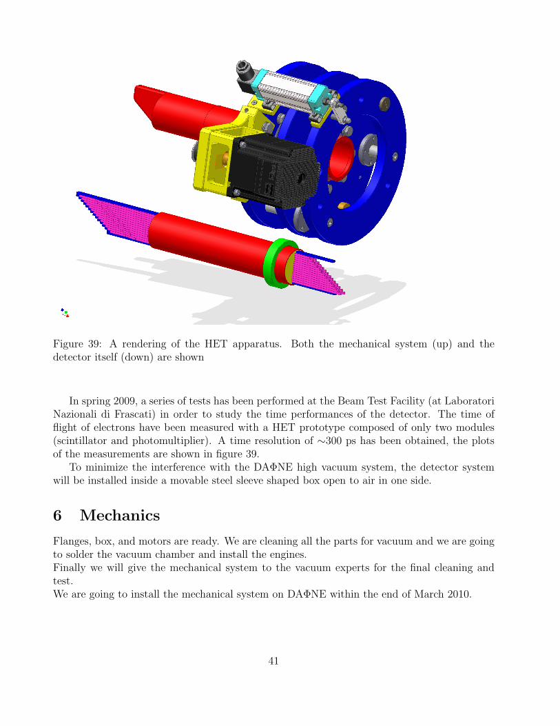
Figure 39: A rendering of the HET apparatus. Both the mechanical system (up) and thedetector itself (down) are shown

In spring 2009, a series of tests has been performed at the Beam Test Facility (at LaboratoriNazionali di Frascati) in order to study the time performances of the detector. The time offlight of electrons have been measured with a HET prototype composed of only two modules(scintillator and photomultiplier). A time resolution of ∼300 ps has been obtained, the plotsof the measurements are shown in figure 39.

To minimize the interference with the DAΦNE high vacuum system, the detector systemwill be installed inside a movable steel sleeve shaped box open to air in one side.

6 Mechanics

Flanges, box, and motors are ready. We are cleaning all the parts for vacuum and we are goingto solder the vacuum chamber and install the engines.Finally we will give the mechanical system to the vacuum experts for the final cleaning andtest.We are going to install the mechanical system on DAΦNE within the end of March 2010.

41

7 Slow Control

We have to monitor the efficiency of the PMTs and compensate (as much as possible) the ageingof the photocathode by increasing the high voltage supply. An automatic system, controlledvia Ethernet, is being developed.The Slow Control system will be structured as follows:

• A pulsed LED controlled by a linear current generator (already tested successfully);

• 32 optical fibres to bring exactly the same light to the each PMTs;

• A 32 channels CAEN VME QDC to acquire the spectrum of every single PMT;

• A VME board with a PIC microcontroller to monitor the efficiency of the PMTs (withthe procedure prevously described) and consequently change the HV supplied.

In case of serious damage of a PMT it can be easily replaced thanks to the mechanical structurethat is being designed.

8 Frontend Electronics

The frontend board is designed. It is composed by

• A fast buffer: LMH6559;

• An Amplifier: LMH6703;

• Two voltage regulators: MC78LC00 and MIC5270;

• A thermometer TC1047A.

The frontend board will provide an analog signal to the Data Acquisition board which isembedding the discriminators (LMH7324). This part of the electronics chain has being testedyielding excellent results: the output signal has a rise time shorter than 0.5 ns.

9 Data Acquisition

The signals come from the HET detector, DAΦNE (fiducial) and KLOE (Trigger and ACQlogic); Acquisition logic (TDC) has been implemented inside the FPGA; A microcomputer,inside a Virtex5 FPGA, handles the communication with KLOE DAQ via the VME bus.As the HET detector is placed far away from the IP, we need to keep track of the number beambunches, i.e. we need to count them. Thus we must distinguish to consecutive bunches: weneed a time resolution ¡ 1 ns; The input stage has been tested (4-phase DCM - 0.5ns); We areable to reach such a time resolution with 500 MHz clock using a DCM and several delay lines.The 8-phase DCM (0.25 ns) has been developed and is currently under test. The Linux OS forthe Virtex5 is being configured and VME Drivers (provided by Roma3) are being adapted tofit Virtex5 board. The board itself is currently being designed, and will be built and tested inthe next few months.

42

9.1 HET Cost Estimate

In the following table we report the cost estimate for the two HET detectors.

Item cost (kEuro)Mechanics 3860 Plastic Scintillators 1060 Hamamatsu MPPC 3x3 mm2 25HV supply + Cables 10Front-End electronics 143 Virtex5 142 Motorola 8Total 119

Table 6: Cost estimate for the HET detectors

43

10 Summary and Time schedule

44

!"#$%#&&# '" (#)**

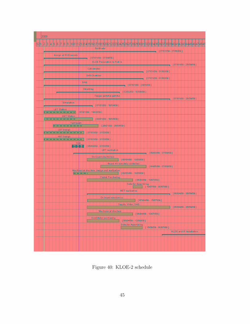
+,-./0

12314315/41340315

6#$7 8

Figure 40: KLOE-2 schedule

45

References

[1] S. J. Brodsky, T. Kinoshita and H. Terazawa, Phys. Rev. Lett. 25, 972 (1970).

[2] see the review by M. R. Pennington, [arXiv:hep-ph/0511146] and reference therein.

[3] H. Marsiske et al. (Crystal Ball Collab.), Phys. Rev. D 41, 3324 (1990).

[4] G. Alexander et al., Nuovo Cimento 107A, 837 (1994); F. Anulli et al., The secondDAΦNE Physics Handbook, Vol. II, eds. L. Maiani, G. Pancheri, and N. Paver (1995),p. 607.

[5] I. Caprini, G. Colangelo and H. Leutwyler, [arXiv:hep-ph/0512364].

[6] E.M. Aitala (E791 Collab.), Phys. Rev. Lett. 86,770 (2001).

[7] M. Ablikim et al. (BES Collab.), Phys. Lett. B598, 149 (2004).

[8] A. Deandrea and A.D. Polosa, Phys. Rev. Lett. 86, 216 (2001); S. Gardner and U. Meissner,Phys. Rev. D65, 094004 (2002); I. Bigi, [arXiv:hep-ph/0601167].

[9] B. Aubert et al. (BaBar Collab.), Phys. Rev. Lett. 95, 121802 (2005).

[10] F. Nguyen, F. Piccinini and A.D. Polosa, Eur. Phys. J. C47, 65 (2006).

[11] S. J. Brodsky, T. Kinoshita and H. Terazawa, Phys. Rev. D 4, 1532 (1971).

[12] A. Bramon, R. Escribano and M. D. Scadron, Eur. Phys. J. C 7, 271 (1999).

[13] E. Kou, Phys. Rev. D 63, 054027 (2001) .

[14] F. Ambrosino et al. [KLOE Collaboration], Phys. Lett. B 648, 267 (2007).

[15] F. Ambrosino et al., Eur. Phys. J. C50, 729 (2007).

[16] F. Jegerlehner and A. Nyffeler, “The Muon g-2”, arXiv:0902.3360 [hep-ph].

[17] E. Abouzaid et al. [KTeV Collaboration], Phys. Rev. D 75 (2007) 012004

[18] A. E. Dorokhov, Nucl. Phys. Proc. Suppl. 181-182 (2008) 37.

[19] T. Oest et al. (JADE Collab.), Z. Phys. C 47, 343 (1990).

[20] J. Gasser, M.A. Ivanov and M. Sainio, Nucl. Phys. B728, 31 (2005); see also S. Bellucci, J.Gasser and M. Sainio Nucl. Phys. B423, 80 (1994); erratum-ibid. B431, 413-414 (1994).

[21] M. R. Pennington, The second DAΦNE Physics Handbook, eds. L. Maiani, G. Pancheri,and N. Paver (1995), p. 531.

[22] A. Courau, SLAC - PUB - 3363 (1984).

[23] http://mad.web.cern.ch/mad

46

[24] http://www.pp.rhul.ac.uk/ malton/bdsim.

[25] J. Carter, I. Agapov, G. A. Blair and O. Dadoun, Pramana 69, 1133 (2007).

[26] L. Quintieri et al., preprint LNF-09/03 (IR).

[27] S. Uehara, private communications; for details on TREPS seehttp:://belle.kek.jp/ uehara/treps-readme.html.

[28] A. Bartalini et al. Eur. Phys. J. A26, 399 (2005).

[29] L.M. Barone et al., Nucl. Instr. Meth. A562, 76-84 (2006)

[30] ........

[31] M.Adinolfi et al. [KLOE Collaboration], Nucl. Instr. Methods A482, 364-386 (2002).

47