Statistical efficiency of curve fitting algorithms

N. Chernov and C. LesortDepartment of Mathematics

University of Alabama at BirminghamBirmingham, AL 35294, USA

March 20, 2003

Abstract

We study the problem of fitting parametrized curves to noisy data. Undercertain assumptions (known as Cartesian and radial functional models), we deriveasymptotic expressions for the bias and the covariance matrix of the parameterestimates. We also extend Kanatani’s version of the Cramer-Rao lower bound,which he proved for unbiased estimates only, to more general estimates that includemany popular algorithms (most notably, the orthogonal least squares and algebraicfits). We then show that the gradient-weighted algebraic fit is statistically efficientand describe all other statistically efficient algebraic fits.

Keywords: least squares fit, curve fitting, circle fitting, algebraic fit, Rao-Cramerbound, efficiency, functional model.

1 Introduction

In many applications one fits a parametrized curve described by an implicit equationP (x, y; Θ) = 0 to experimental data (xi, yi), i = 1, . . . , n. Here Θ denotes the vector ofunknown parameters to be estimated. Typically, P is a polynomial in x and y, and itscoefficients are unknown parameters (or functions of unknown parameters). For example,a number of recent publications [2, 10, 11, 16, 19] are devoted to the problem of fittingquadrics Ax2+Bxy+Cy2+Dx+Ey+F = 0, in which case Θ = (A,B,C, D,E, F ) is theparameter vector. The problem of fitting circles, given by equation (x−a)2+(y−b)2−R2 =0 with three parameters a, b, R, also attracted attention [8, 14, 15, 18].

We consider here the problem of fitting general curves given by implicit equationsP (x, y; Θ) = 0 with Θ = (θ1, . . . , θk) being the parameter vector. Our goal is to in-vestigate statistical properties of various fitting algorithms. We are interested in theirbiasedness, covariance matrices, and the Cramer-Rao lower bound.

1

First, we specify our model. We denote by Θ the true value of Θ. Let (xi, yi),i = 1, . . . , n, be some points lying on the true curve P (x, y; Θ) = 0. Experimentallyobserved data points (xi, yi), i = 1, . . . , n, are perceived as random perturbations of thetrue points (xi, yi). We use notation xi = (xi, yi)

T and xi = (xi, yi)T , for brevity. The

random vectors ei = xi − xi are assumed to be independent and have zero mean. Twospecific assumptions on their probability distribution can be made, see [4]:

Cartesian model: Each ei is a two-dimensional normal vector with covariance matrixσ2

i I, where I is the identity matrix.

Radial model: ei = ξini where ξi is a normal random variable N (0, σ2i ), and ni is a

unit normal vector to the curve P (x, y; Θ) = 0 at the point xi.

Our analysis covers both models, Cartesian and radial. For simplicity, we assume thatσ2

i = σ2 for all i, but note that our results can be easily generalized to arbitrary σ2i > 0.

Concerning the true points xi, i = 1, . . . , n, two assumptions are possible. Manyresearchers [6, 13, 14] consider them as fixed, but unknown, points on the true curve.In this case their coordinates (xi, yi) can be treated as additional parameters of themodel (nuisance parameters). Chan [6] and others [3, 4] call this assumption a functionalmodel. Alternatively, one can assume that the true points xi are sampled from the curveP (x, y; Θ) = 0 according to some probability distribution on it. This assumption isreferred to as a structural model [3, 4]. We only consider the functional model here.

It is easy to verify that maximum likelihood estimation of the parameter Θ for thefunctional model is given by the orthogonal least squares fit (OLSF), which is based onminimization of the function

F1(Θ) =n∑

i=1

[di(Θ)]2 (1.1)

where di(Θ) denotes the distance from the point xi to the curve P (x, y; Θ) = 0. TheOLSF is the method of choice in practice, especially when one fits simple curves suchas lines and circles. However, for more general curves the OLSF becomes intractable,because the precise distance di is hard to compute. For example, when P is a genericquadric (ellipse or hyperbola), the computation of di is equivalent to solving a polynomialequation of degree four, and its direct solution is known to be numerically unstable, see[2, 11] for more detail. Then one resorts to various approximations. It is often convenientto minimize

F2(Θ) =n∑

i=1

[P (xi, yi; Θ)]2 (1.2)

instead of (1.1). This method is referred to as a (simple) algebraic fit (AF), in this caseone calls |P (xi, yi; Θ)| the algebraic distance [2, 10, 11] from the point (xi, yi) to thecurve. The AF is computationally cheaper than the OLSF, but its accuracy is oftenunacceptable, see below.

2

The simple AF (1.2) can be generalized to a weighted algebraic fit, which is based onminimization of

F3(Θ) =n∑

i=1

wi [P (xi, yi; Θ)]2 (1.3)

where wi = w(xi, yi; Θ) are some weights, which may balance (1.2) and improve itsperformance. One way to define weights wi results from a linear approximation to di:

di ≈ |P (xi, yi; Θ)|‖∇xP (xi, yi; Θ)‖

where ∇xP = (∂P/∂x, ∂P/∂y) is the gradient vector, see [20]. Then one minimizes thefunction

F4(Θ) =n∑

i=1

[P (xi, yi; Θ)]2

‖∇xP (xi, yi; Θ)‖2(1.4)

This method is called the gradient weighted algebraic fit (GRAF). It is a particular caseof (1.3) with wi = 1/‖∇xP (xi, yi; Θ)‖2.

The GRAF is known since at least 1974 [21] and recently became standard for polyno-mial curve fitting [20, 16, 10]. The computational cost of GRAF depends on the functionP (x, y; Θ), but, generally, the GRAF is much faster than the OLSF. It is also knownfrom practice that the accuracy of GRAF is almost as good as that of the OLSF, andour analysis below confirms this fact. The GRAF is often claimed to be a statisticallyoptimal weighted algebraic fit, and we will prove this fact as well.

Not much has been published on statistical properties of the OLSF and algebraicfits, apart from the simplest case of fitting lines and hyperplanes [12]. Chan [6], Bermanand Culpin [4] investigated circle fitting by the OLSF and the simple algebraic fit (1.2)assuming the structural model. Kanatani [13, 14] used the Cartesian functional modeland considered a general curve fitting problem. He established an analogue of the Rao-Cramer lower bound for unbiased estimates of Θ, which we call here Kanatani-Cramer-Rao (KCR) lower bound. He also showed that the covariance matrices of the OLSF andthe GRAF attain, to the leading order in σ, his lower bound. We note, however, that inmost cases the OLSF and algebraic fits are biased [4, 5], hence the KCR lower bound, asit is derived in [13, 14], does not immediately apply to these methods.

In this paper we extend the KCR lower bound to biased estimates, which include theOLSF and all weighted algebraic fits. We prove the KCR bound for estimates satisfyingthe following mild assumption:

Precision assumption. For precise observations (when xi = xi for all 1 ≤ i ≤ n), theestimate Θ is precise, i.e.

Θ(x1, . . . , xn) = Θ (1.5)

It is easy to check that the OLSF and algebraic fits (1.3) satisfy this assumption. Wewill also show that all unbiased estimates of Θ satisfy (1.5).

We then prove that the GRAF is, indeed, a statistically efficient fit, in the sense thatits covariance matrix attains, to the leading order in σ, the KCR lower bound. On the

3

other hand, rather surprisingly, we find that GRAF is not the only statistically efficientalgebraic fit, and we describe all statistically efficient algebraic fits. Finally, we show thatKanatani’s theory and our extension to it remain valid for the radial functional model.Our conclusions are illustrated by numerical experiments on circle fitting algorithms.

2 Kanatani-Cramer-Rao lower bound

Recall that we have adopted the functional model, in which the true points xi, 1 ≤ i ≤n, are fixed. This automatically makes the sample size n fixed, hence, many classicalconcepts of statistics, such as consistency and asymptotic efficiency (which require takingthe limit n → ∞) lose their meaning. It is customary, in the studies of the functionalmodel of the curve fitting problem, to take the limit σ → 0 instead of n → ∞, cf.[13, 14]. This is, by the way, not unreasonable from the practical point of view: in manyexperiments, n is rather small and cannot be (easily) increased, so the limit n → ∞ isof little interest. On the other hand, when the accuracy of experimental observations ishigh (thus, σ is small), the limit σ → 0 is quite appropriate.

Now, let Θ(x1, . . . ,xn) be an arbitrary estimate of Θ satisfying the precision assump-tion (1.5). In our analysis we will always assume that all the underlying functions areregular (continuous, have finite derivatives, etc.), which is a standard assumption [13, 14].

The mean value of the estimate Θ is

E(Θ) =∫· · ·

∫Θ(x1, . . . ,xn)

n∏

i=1

f(xi) dx1 · · · dxn (2.1)

where f(xi) is the probability density function for the random point xi, as specified bya particular model (Cartesian or radial).

We now expand the estimate Θ(x1, . . . ,xn) into a Taylor series about the true point(x1, . . . , xn) remembering (1.5):

Θ(x1, . . . ,xn) = Θ +n∑

i=1

Θi × (xi − xi) +O(σ2) (2.2)

whereΘi = ∇xi

Θ(x1, . . . , xn), i = 1, . . . , n (2.3)

and ∇xistands for the gradient with respect to the variables xi, yi. In other words, Θi is

a k × 2 matrix of partial derivatives of the k components of the function Θ with respectto the two variables xi and yi, and this derivative is taken at the point (x1, . . . , xn),

Substituting the expansion (2.2) into (2.1) gives

E(Θ) = Θ +O(σ2) (2.4)

since E(xi − xi) = 0. Hence, the bias of the estimate Θ is of order σ2.

4

It easily follows from the expansion (2.2) that the covariance matrix of the estimateΘ is given by

CΘ =n∑

i=1

ΘiE[(xi − xi)(xi − xi)T ]ΘT

i +O(σ4)

(it is not hard to see that the cubical terms O(σ3) vanish because the normal randomvariables with zero mean also have zero third moment, see also [13]). Now, for theCartesian model

E[(xi − xi)(xi − xi)T ] = σ2I

and for the radial model

E[(xi − xi)(xi − xi)T ] = σ2nin

Ti

where ni is a unit normal vector to the curve P (x, y; Θ) = 0 at the point xi. Then weobtain

CΘ = σ2n∑

i=1

ΘiΛiΘTi +O(σ4) (2.5)

where Λi = I for the Cartesian model and Λi = ninTi for the radial model.

Lemma. We have ΘininTi ΘT

i = ΘiΘTi for each i = 1, . . . , n. Hence, for both models,

Cartesian and radial, the matrix CΘ is given by the same expression:

CΘ = σ2n∑

i=1

ΘiΘTi +O(σ4) (2.6)

This lemma is proved in Appendix.Our next goal is now to find a lower bound for the matrix

D1 :=n∑

i=1

ΘiΘTi (2.7)

Following [13, 14], we consider perturbations of the parameter vector Θ + δΘ and thetrue points xi + δxi satisfying two constraints. First, since the true points must belongto the true curve, P (xi; Θ) = 0, we obtain, by the chain rule,

〈∇x P (xi; Θ), δxi〉+ 〈∇ΘP (xi; Θ), δΘ〉 = 0 (2.8)

where 〈·, ·〉 stands for the scalar product of vectors. Second, since the identity (1.5) holdsfor all Θ, we get

n∑

i=1

Θi δxi = δΘ (2.9)

by using the notation (2.3).

5

Now we need to find a lower bound for the matrix (2.7) subject to the constraints(2.8) and (2.9). That bound follows from a general theorem in linear algebra:

Theorem (Linear Algebra). Let n ≥ k ≥ 1 and m ≥ 1. Suppose n nonzero vectorsui ∈ IRm and n nonzero vectors vi ∈ IRk are given, 1 ≤ i ≤ n. Consider k ×m matrices

Xi =viu

Ti

uTi ui

for 1 ≤ i ≤ n, and k × k matrix

B =n∑

i=1

XiXTi =

n∑

i=1

vivTi

uTi ui

Assume that the vectors v1, . . . , vn span IRk (hence B is nonsingular). We say that a setof n matrices A1, . . . , An (each of size k ×m) is proper if

n∑

i=1

Aiwi = r (2.10)

for any vectors wi ∈ IRm and r ∈ IRk such that

uTi wi + vT

i r = 0 (2.11)

for all 1 ≤ i ≤ n. Then for any proper set of matrices A1, . . . , An the k × k matrixD =

∑ni=1 AiA

Ti is bounded from below by B−1 in the sense that D − B−1 is a positive

semidefinite matrix. The equality D = B−1 holds if and only if Ai = −B−1Xi for alli = 1, . . . , n.

This theorem is, probably, known, but we provide a full proof in Appendix, for thesake of completeness.

As a direct consequence of the above theorem we obtain the lower bound for ourmatrix D1:

Theorem (Kanatani-Cramer-Rao lower bound). We have D1 ≥ Dmin, in the sensethat D1 −Dmin is a positive semidefinite matrix, where

D−1min =

n∑

i=1

(∇ΘP (xi; Θ))(∇ΘP (xi; Θ))T

‖∇x P (xi; Θ)‖2(2.12)

In view of (2.6) and (2.7), the above theorem says that the lower bound for thecovariance matrix CΘ is, to the leading order,

CΘ ≥ Cmin = σ2Dmin (2.13)

6

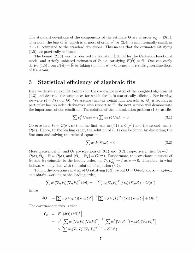
The standard deviations of the components of the estimate Θ are of order σΘ = O(σ).

Therefore, the bias of Θ, which is at most of order σ2 by (2.4), is infinitesimally small, asσ → 0, compared to the standard deviations. This means that the estimates satisfying(1.5) are practically unbiased.

The bound (2.13) was first derived by Kanatani [13, 14] for the Cartesian functionalmodel and strictly unbiased estimates of Θ, i.e. satisfying E(Θ) = Θ. One can easilyderive (1.5) from E(Θ) = Θ by taking the limit σ → 0, hence our results generalize thoseof Kanatani.

3 Statistical efficiency of algebraic fits

Here we derive an explicit formula for the covariance matrix of the weighted algebraic fit(1.3) and describe the weights wi for which the fit is statistically efficient. For brevity,we write Pi = P (xi, yi; Θ). We assume that the weight function w(x, y, ; Θ) is regular, inparticular has bounded derivatives with respect to Θ, the next section will demonstratethe importance of this condition. The solution of the minimization problem (1.3) satisfies

∑P 2

i ∇Θwi + 2∑

wi Pi∇ΘPi = 0 (3.1)

Observe that Pi = O(σ), so that the first sum in (3.1) is O(σ2) and the second sum isO(σ). Hence, to the leading order, the solution of (3.1) can be found by discarding thefirst sum and solving the reduced equation

∑wi Pi∇ΘPi = 0 (3.2)

More precisely, if Θ1 and Θ2 are solutions of (3.1) and (3.2), respectively, then Θ1− Θ =O(σ), Θ2− Θ = O(σ), and ‖Θ1− Θ2‖ = O(σ2). Furthermore, the covariance matrices ofΘ1 and Θ2 coincide, to the leading order, i.e. CΘ1

C−1

Θ2→ I as σ → 0. Therefore, in what

follows, we only deal with the solution of equation (3.2).To find the covariance matrix of Θ satisfying (3.2) we put Θ = Θ+δΘ and xi = xi+δxi

and obtain, working to the leading order,∑

wi(∇ΘPi)(∇ΘPi)T (δΘ) = −∑

wi(∇xPi)T (δxi) (∇ΘPi) +O(σ2)

hence

δΘ = −[∑

wi(∇ΘPi)(∇ΘPi)T]−1 [∑

wi(∇xPi)T (δxi) (∇ΘPi)

]+O(σ2)

The covariance matrix is then

CΘ = E[(δΘ) (δΘ)T

]

= σ2[∑

wi(∇ΘPi)(∇ΘPi)T]−1 [∑

w2i ‖∇xPi‖2(∇ΘPi)(∇ΘPi)

T]

×[∑

wi(∇ΘPi)(∇ΘPi)T]−1

+O(σ3)

7

Denote by D2 the principal factor here, i.e.

D2 =[∑

wi(∇ΘPi)(∇ΘPi)T]−1 [∑

w2i ‖∇xPi‖2(∇ΘPi)(∇ΘPi)

T] [∑

wi(∇ΘPi)(∇ΘPi)T]−1

The following theorem establishes a lower bound for D2:

Theorem. We have D2 ≥ Dmin, in the sense that D2 − Dmin is a positive semidefinitematrix, where Dmin is given by (2.12). The equality D2 = Dmin holds if and only if wi =const/‖∇x Pi‖2 for all i = 1, . . . , n. In other words, an algebraic fit (1.3) is statisticallyefficient if and only if the weight function w(x, y; Θ) satisfies

w(x, y; Θ) =c(Θ)

‖∇x P (x, y; Θ)‖2(3.3)

for all triples x, y, Θ such that P (x, y; Θ) = 0. Here c(Θ) may be an arbitrary functionof Θ.

The bound D2 ≥ Dmin here is a particular case of the previous theorem. It also canbe obtained directly from the linear algebra theorem if one sets ui = ∇xPi, vi = ∇ΘPi,and

Ai = −wi

n∑

j=1

wj(∇ΘPj)(∇ΘPj)T

−1

(∇ΘPi) (∇xPi)T

for 1 ≤ i ≤ n.The expression (3.3) characterizing the efficiency, follows from the last claim in the

linear algebra theorem.

4 Circle fit

Here we illustrate our conclusions by the relatively simple problem of fitting circles. Thecanonical equation of a circle is

(x− a)2 + (y − b)2 −R2 = 0 (4.1)

and we need to estimate three parameters a, b, R. The simple algebraic fit (1.2) takesform

F2(a, b, R) =n∑

i=1

[(xi − a)2 + (yi − b)2 −R2]2 → min (4.2)

and the weighted algebraic fit (1.3) takes form

F3(a, b, R) =n∑

i=1

wi[(xi − a)2 + (yi − b)2 −R2]2 → min (4.3)

8

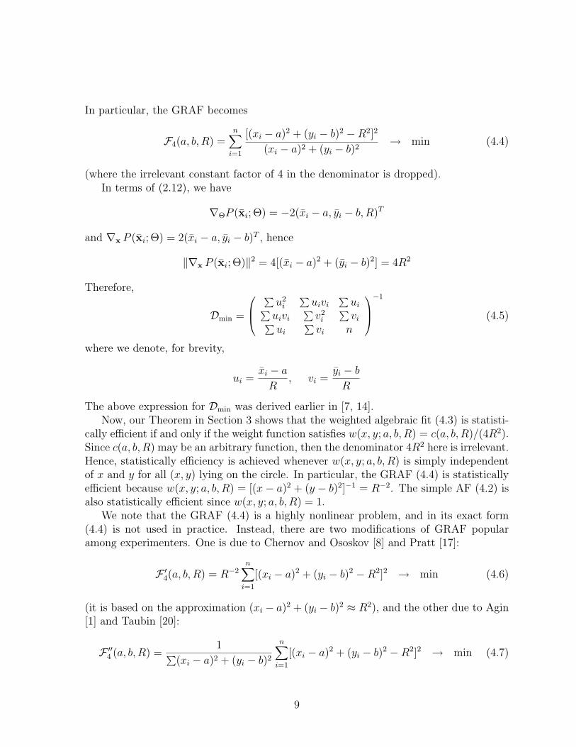
In particular, the GRAF becomes

F4(a, b, R) =n∑

i=1

[(xi − a)2 + (yi − b)2 −R2]2

(xi − a)2 + (yi − b)2→ min (4.4)

(where the irrelevant constant factor of 4 in the denominator is dropped).In terms of (2.12), we have

∇ΘP (xi; Θ) = −2(xi − a, yi − b, R)T

and ∇x P (xi; Θ) = 2(xi − a, yi − b)T , hence

‖∇x P (xi; Θ)‖2 = 4[(xi − a)2 + (yi − b)2] = 4R2

Therefore,

Dmin =

∑u2

i

∑uivi

∑ui∑

uivi∑

v2i

∑vi∑

ui∑

vi n

−1

(4.5)

where we denote, for brevity,

ui =xi − a

R, vi =

yi − b

R

The above expression for Dmin was derived earlier in [7, 14].Now, our Theorem in Section 3 shows that the weighted algebraic fit (4.3) is statisti-

cally efficient if and only if the weight function satisfies w(x, y; a, b, R) = c(a, b, R)/(4R2).Since c(a, b, R) may be an arbitrary function, then the denominator 4R2 here is irrelevant.Hence, statistically efficiency is achieved whenever w(x, y; a, b, R) is simply independentof x and y for all (x, y) lying on the circle. In particular, the GRAF (4.4) is statisticallyefficient because w(x, y; a, b, R) = [(x− a)2 + (y − b)2]−1 = R−2. The simple AF (4.2) isalso statistically efficient since w(x, y; a, b, R) = 1.

We note that the GRAF (4.4) is a highly nonlinear problem, and in its exact form(4.4) is not used in practice. Instead, there are two modifications of GRAF popularamong experimenters. One is due to Chernov and Ososkov [8] and Pratt [17]:

F ′4(a, b, R) = R−2

n∑

i=1

[(xi − a)2 + (yi − b)2 −R2]2 → min (4.6)

(it is based on the approximation (xi − a)2 + (yi − b)2 ≈ R2), and the other due to Agin[1] and Taubin [20]:

F ′′4 (a, b, R) =

1∑(xi − a)2 + (yi − b)2

n∑

i=1

[(xi − a)2 + (yi − b)2 −R2]2 → min (4.7)

9

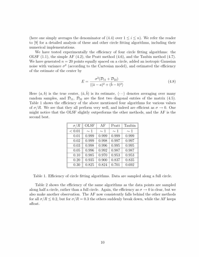
(here one simply averages the denominator of (4.4) over 1 ≤ i ≤ n). We refer the readerto [9] for a detailed analysis of these and other circle fitting algorithms, including theirnumerical implementations.

We have tested experimentally the efficiency of four circle fitting algorithms: theOLSF (1.1), the simple AF (4.2), the Pratt method (4.6), and the Taubin method (4.7).We have generated n = 20 points equally spaced on a circle, added an isotropic Gaussiannoise with variance σ2 (according to the Cartesian model), and estimated the efficiencyof the estimate of the center by

E =σ2(D11 +D22)

〈(a− a)2 + (b− b)2〉 (4.8)

Here (a, b) is the true center, (a, b) is its estimate, 〈· · ·〉 denotes averaging over manyrandom samples, and D11, D22 are the first two diagonal entries of the matrix (4.5).Table 1 shows the efficiency of the above mentioned four algorithms for various valuesof σ/R. We see that they all perform very well, and indeed are efficient as σ → 0. Onemight notice that the OLSF slightly outperforms the other methods, and the AF is thesecond best.

σ/R OLSF AF Pratt Taubin

< 0.01 ∼ 1 ∼ 1 ∼ 1 ∼ 10.01 0.999 0.999 0.999 0.9990.02 0.999 0.998 0.997 0.9970.03 0.998 0.996 0.995 0.9950.05 0.996 0.992 0.987 0.9870.10 0.985 0.970 0.953 0.9530.20 0.935 0.900 0.837 0.8350.30 0.825 0.824 0.701 0.692

Table 1. Efficiency of circle fitting algorithms. Data are sampled along a full circle.

Table 2 shows the efficiency of the same algorithms as the data points are sampledalong half a circle, rather than a full circle. Again, the efficiency as σ → 0 is clear, but wealso make another observation. The AF now consistently falls behind the other methodsfor all σ/R ≤ 0.2, but for σ/R = 0.3 the others suddenly break down, while the AF keepsafloat.

10

σ/R OLSF AF Pratt Taubin

< 0.01 ∼ 1 ∼ 1 ∼ 1 ∼ 10.01 0.999 0.996 0.999 0.9990.02 0.997 0.983 0.997 0.9970.03 0.994 0.961 0.992 0.9920.05 0.984 0.902 0.978 0.9780.10 0.935 0.720 0.916 0.9160.20 0.720 0.493 0.703 0.6910.30 0.122 0.437 0.186 0.141

Table 2. Efficiency of circle fitting algorithms with data sampled along half a circle.

The reason of the above turnaround is that at large noise the data points may occa-sionally line up along a circular arc of a very large radius. Then the OLSF, Pratt andTaubin dutifully return a large circle whose center lies far away, and such fits blow upthe denominator of (4.8), a typical effect of large outliers. On the contrary, the AF isnotoriously known for its systematic bias toward smaller circles [8, 11, 17], hence whileit is less accurate than other fits for typical random samples, its bias safeguards it fromlarge outliers.

This behavior is even more pronounced when the data are sampled along quarter1 ofa circle (Table 3). We see that the AF is now far worse than the other fits for σ/R < 0.1but the others characteristically break down at some point (σ/R = 0.1).

σ/R OLSF AF Pratt Taubin

0.01 0.997 0.911 0.997 0.9970.02 0.977 0.722 0.978 0.9780.03 0.944 0.555 0.946 0.9460.05 0.837 0.365 0.843 0.8420.10 0.155 0.275 0.163 0.158

Table 3. Data are sampled along a quarter of a circle.

It is interesting to test smaller circular arcs, too. Figure 1 shows a color-coded diagramof the efficiency of the OLSF and the AF for arcs from 0o to 50o and variable σ (we setσ = ch, where h is the height of the circular arc, see Fig. 2, and c varies from 0 to 0.5).The efficiency of the Pratt and Taubin is virtually identical to that of the OLSF, so it isnot shown here. We see that the OLSF and AF are efficient as σ → 0 (both squares inthe diagram get white at the bottom), but the AF loses its efficiency at moderate levels

1All our algorithms are invariant under simple geometric transformations such as translations, rota-tions and similarities, hence our experimental results do not depend on the choice of the circle, its size,and the part of the circle the data are sampled from.

11

of noise (c > 0.1), while the OLSF remains accurate up to c = 0.3 after which it rathersharply breaks down.

5040302010

0.5

0.4

0.3

0.2

0.1

0

c

Arc in degrees5040302010

0.5

0.4

0.3

0.2

0.1

0

c

Arc in degrees

1.00.90.80.70.60.50.40.30.20.10

Figure 1: The efficiency of the simple OLSF (left) and the AF (center). The bar on theright explains color codes.

The following analysis sheds more light on the behavior of the circle fitting algorithms.When the curvature of the arc decreases, the center coordinates a, b and the radius Rgrow to infinity and their estimates become highly unreliable. In that case the circleequation (4.1) can be converted to a more convenient algebraic form

A(x2 + y2) + Bx + Cy + D = 0 (4.9)

with an additional constrain on the parameters: B2+C2−4AD = 1. This parametrizationwas used in [17, 11], and analyzed in detail in [9]. We note that the original parameterscan be recovered via a = −B/2A, b = −C/2A, and R = (2 |A|)−1. The new parametriza-tion (4.9) is safe to use for arcs with arbitrary small curvature: the parameters A,B, C, Dremain bounded and never develop singularities, see [9]. Even as the curvature vanishes,we simply get A = 0, and the equation (4.9) represents a line Bx + Cy + D = 0.

h

chσ =

Figure 2: The height of an arc, h, and our formula for σ.

In terms of the new parameters A,B, C, D, the weighted algebraic fit (1.3) takes form

F3(A,B,C,D) =n∑

i=1

wi[A(x2 + y2) + Bx + Cy + D]2 → min (4.10)

12

(under the constraint B2+C2−4AD = 1). Converting the AF (4.2) to the new parametersgives

F2(A,B, C, D) =n∑

i=1

A−2[A(x2 + y2) + Bx + Cy + D]2 → min (4.11)

which corresponds to the weight function w = 1/A2. The Pratt method (4.6) turns to

F4(A,B,C,D) =n∑

i=1

[A(x2 + y2) + Bx + Cy + D]2 → min (4.12)

We now see why the AF is unstable and inaccurate for arcs with small curvature: itsweight function w = 1/A2 develops a singularity (it explodes) in the limit A → 0. Recallthat, in our derivation of the statistical efficiency theorem (Section 3), we assumed thatthe weight function was regular (had bounded derivatives). This assumption is clearlyviolated by the AF (4.11). On the contrary, the Pratt fit (4.12) uses a safe choice w = 1and thus behaves decently on arcs with small curvature, see next.

5040302010

0.5

0.4

0.3

0.2

0.1

0

c

Arc in degrees5040302010

0.5

0.4

0.3

0.2

0.1

0

c

Arc in degrees

1.00.90.80.70.60.50.40.30.20.10

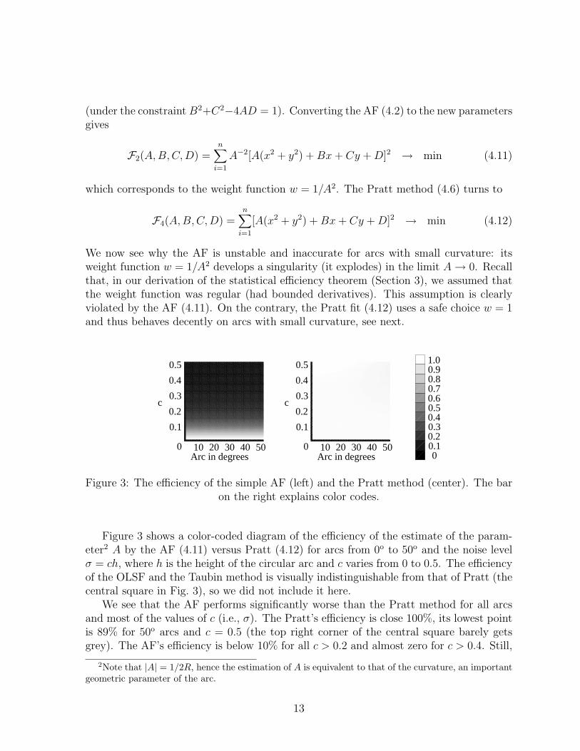
Figure 3: The efficiency of the simple AF (left) and the Pratt method (center). The baron the right explains color codes.

Figure 3 shows a color-coded diagram of the efficiency of the estimate of the param-eter2 A by the AF (4.11) versus Pratt (4.12) for arcs from 0o to 50o and the noise levelσ = ch, where h is the height of the circular arc and c varies from 0 to 0.5. The efficiencyof the OLSF and the Taubin method is visually indistinguishable from that of Pratt (thecentral square in Fig. 3), so we did not include it here.

We see that the AF performs significantly worse than the Pratt method for all arcsand most of the values of c (i.e., σ). The Pratt’s efficiency is close 100%, its lowest pointis 89% for 50o arcs and c = 0.5 (the top right corner of the central square barely getsgrey). The AF’s efficiency is below 10% for all c > 0.2 and almost zero for c > 0.4. Still,

2Note that |A| = 1/2R, hence the estimation of A is equivalent to that of the curvature, an importantgeometric parameter of the arc.

13

the AF remains efficient as σ → 0 (as the tiny white strip at the bottom of the left squareproves), but its efficiency can be only counted on when σ is extremely small.

Our analysis demonstrates that the choice of the weights wi in the weighted algebraicfit (1.3) should be made according to our theorem in Section 3, and, in addition, oneshould avoid singularities in the domain of parameters.

Appendix

Here we prove the theorem of linear algebra stated in Section 2. For the sake of clarity,we divide our proof into small lemmas:

Lemma 1. The matrix B is indeed nonsingular.Proof. If Bz = 0 for some nonzero vector z ∈ IRk, then 0 = zT Bz =

∑ni=1(v

Ti z)2/‖ui‖2,

hence vTi z = 0 for all 1 ≤ i ≤ k, a contradiction.

Lemma 2. If a set of n matrices A1, . . . , An is proper, then rank(Ai) ≤ 1. Furthermore,each Ai is given by Ai = ziu

Ti for some vector zi ∈ IRk, and the vectors z1, . . . , zn satisfy∑n

i=1 zivTi = −I where I is the k × k identity matrix. The converse is also true.

Proof. Let vectors w1, . . . , wn and r satisfy the requirements (2.10) and (2.11) of thetheorem. Consider the orthogonal decomposition wi = ciui + w⊥

i where w⊥i is perpendic-

ular to ui, i.e. uTi w⊥

i = 0. Then the constraint (2.11) can be rewritten as

ci = − vTi r

uTi ui

(A.1)

for all i = 1, . . . , n and (2.10) takes form

n∑

i=1

ciAiui +n∑

i=1

Aiw⊥i = r (A.2)

We conclude that Aiw⊥i = 0 for every vector w⊥

i orthogonal to ui, hence Ai has a (k−1)-dimensional kernel, so indeed its rank is zero or one. If we denote zi = Aiui/‖ui‖2, weobtain Ai = ziu

Ti . Combining this with (A.1)-(A.2) gives

r = −n∑

i=1

(vTi r)zi = −

(n∑

i=1

zivTi

)r

Since this identity holds for any vector r ∈ IRk, the expression within parentheses is −I.The converse is obtained by straightforward calculations. Lemma is proved.

Corollary. Let ni = ui/‖ui‖. Then AininTi Ai = AiA

Ti for each i.

This corollary implies our lemma stated in Section 2. We now continue the proof ofthe theorem.

14

Lemma 3. The sets of proper matrices make a linear variety, in the following sense. LetA′

1, . . . , A′n and A′′

1, . . . , A′′n be two proper sets of matrices, then the set A1, . . . , An defined

by Ai = A′i + c(A′′

i − A′i) is proper for every c ∈ IR.

Proof. According to the previous lemma, A′i = z′iu

Ti and A′′

i = z′′i uTi for some vectors

z′i, z′′i , 1 ≤ i ≤ n. Therefore, Ai = ziu

Ti for zi = z′i + c(z′′i − z′i). Lastly,

n∑

i=1

zivTi =

n∑

i=1

z′ivTi + c

n∑

i=1

z′′i vTi − c

n∑

i=1

z′ivTi = −I

Lemma is proved.

Lemma 4. If a set of n matrices A1, . . . , An is proper, then∑n

i=1 AiXTi = −I, where I

is the k × k identity matrix.Proof. By using Lemma 2

∑ni=1 AiX

Ti =

∑ni=1 ziv

Ti = −I. Lemma is proved.

Lemma 5. We have indeed D ≥ B−1.

Proof. For each i = 1, . . . , n consider the 2k × m matrix Yi =

(Ai

Xi

). Using the

previous lemma givesn∑

i=1

Yi YTi =

(D −I−I B

)

By construction, this matrix is positive semidefinite. Hence, the following matrix is alsopositive semidefinite:

(I B−1

0 B−1

) (D −I−I B

) (I 0

B−1 B−1

)=

(D −B−1 0

0 B−1

)

By Sylvester’s theorem, the matrix D −B−1 is positive semidefinite.

Lemma 6. The set of matrices Aoi = −B−1Xi is proper, and for this set we have

D = B−1.Proof. Straightforward calculation.

Lemma 7. If D = B−1 for some proper set of matrices A1, . . . , An, then Ai = Aoi for all

1 ≤ i ≤ n.Proof. Assume that there is a proper set of matrices A′

1, . . . , A′n, different from

Ao1, . . . , A

on, for which D = B−1. Denote δAi = A′

i − Aoi . By Lemma 3, the set of

matrices Ai(γ) = Aoi + γ(δAi) is proper for every real γ. Consider the variable matrix

D(γ) =n∑

i=1

[Ai(γ)][Ai(γ)]T

=n∑

i=1

Aoi (A

oi )

T + γ

(n∑

i=1

Aoi (δAi)

T +n∑

i=1

(δAi)(Aoi )

T

)+ γ2

n∑

i=1

(δAi)(δAi)T

Note that the matrix R =∑n

i=1 Aoi (δAi)

T +∑n

i=1(δAi)(Aoi )

T is symmetric. By Lemma 5we have D(γ) ≥ B−1 for all γ, and by Lemma 6 we have D(0) = B−1. It is then easy

15

to derive that R = 0. Next, the matrix S =∑n

i=1(δAi)(δAi)T is symmetric positive

semidefinite. Since we assumed that D(1) = D(0) = B−1, it is easy to derive that S = 0as well. Therefore, δAi = 0 for every i = 1, . . . , n. The theorem is proved.

References

[1] G.J. Agin, Fitting Ellipses and General Second-Order Curves, Carnegi Mellon Uni-versity, Robotics Institute, Technical Report 81-5, 1981.

[2] S.J. Ahn, W. Rauh, and H.J. Warnecke, Least-squares orthogonal distances fitting ofcircle, sphere, ellipse, hyperbola, and parabola, Pattern Recog., 34, 2001, 2283–2303.

[3] D. A. Anderson, The circular structural model, J. R. Statist. Soc. B, 27, 1981,131–141.

[4] M. Berman and D. Culpin, The statistical behaviour of some least squares estimatorsof the centre and radius of a circle, J. R. Statist. Soc. B, 48, 1986, 183–196.

[5] M. Berman, Large sample bias in least squares estimators of a circular arc center andits radius, Computer Vision, Graphics and Image Processing, 45, 1989, 126–128.

[6] N. N. Chan, On circular functional relationships, J. R. Statist. Soc. B, 27, 1965,45–56.

[7] Y. T. Chan and S. M. Thomas, Cramer-Rao Lower Bounds for Estimation of aCircular Arc Center and Its Radius, Graph. Models Image Proc. 57, 1995, 527–532.

[8] N. I. Chernov and G. A. Ososkov, Effective algorithms for circle fitting, Comp. Phys.Comm. 33, 1984, 329–333.

[9] N. Chernov and C. Lesort, Fitting circles and lines by least squares: theory andexperiment, preprint, available at http://www.math.uab.edu/cl/cl1

[10] W. Chojnacki, M.J. Brooks, and A. van den Hengel, Rationalising the renormalisa-tion method of Kanatani, J. Math. Imaging & Vision, 14, 2001, 21–38.

[11] W. Gander, G.H. Golub, and R. Strebel, Least squares fitting of circles and ellipses,BIT 34, 1994, 558–578.

[12] Recent advances in total least squares techniques and errors-in-variables modeling,Ed. by S. van Huffel, SIAM, Philadelphia, 1997.

[13] K. Kanatani, Statistical Optimization for Geometric Computation: Theory andPractice, Elsevier Science, Amsterdam, 1996.

16

[14] K. Kanatani, Cramer-Rao lower bounds for curve fitting, Graph. Models Image Proc.60, 1998, 93–99.

[15] U.M. Landau, Estimation of a circular arc center and its radius, Computer Vision,Graphics and Image Processing, 38 (1987), 317–326.

[16] Y. Leedan and P. Meer, Heteroscedastic regression in computer vision: Problemswith bilinear constraint, Intern. J. Comp. Vision, 37, 2000, 127–150.

[17] V. Pratt, Direct least-squares fitting of algebraic surfaces, Computer Graphics 21,1987, 145–152.

[18] H. Spath, Least-Squares Fitting By Circles, Computing, 57, 1996, 179–185.

[19] H. Spath, Orthogonal least squares fitting by conic sections, in Recent Advances inTotal Least Squares techniques and Errors-in-Variables Modeling, SIAM, 1997, pp.259–264.

[20] G. Taubin, Estimation Of Planar Curves, Surfaces And Nonplanar Space CurvesDefined By Implicit Equations, With Applications To Edge And Range Image Seg-mentation, IEEE Transactions on Pattern Analysis and Machine Intelligence, 13,1991, 1115–1138.

[21] K. Turner, Computer perception of curved objects using a television camera, Ph.D.Thesis, Dept. of Machine Intelligence, University of Edinburgh, 1974.

17