Sparse Solution of Underdetermined Linear Equations

by Stagewise Orthogonal Matching Pursuit

David L. Donoho 1, Yaakov Tsaig 2, Iddo Drori 1, Jean-Luc Starck 3

March 2006

Abstract

Finding the sparsest solution to underdetermined systems of linear equations y = Φx is NP-hardin general. We show here that for systems with ‘typical’/‘random’ Φ, a good approximation to thesparsest solution is obtained by applying a fixed number of standard operations from linear algebra.

Our proposal, Stagewise Orthogonal Matching Pursuit (StOMP), successively transforms thesignal into a negligible residual. Starting with initial residual r0 = y, at the s-th stage it formsthe ‘matched filter’ ΦT rs−1, identifies all coordinates with amplitudes exceeding a specially-chosenthreshold, solves a least-squares problem using the selected coordinates, and subtracts the least-squares fit, producing a new residual. After a fixed number of stages (e.g. 10), it stops. In contrastto Orthogonal Matching Pursuit (OMP), many coefficients can enter the model at each stage inStOMP while only one enters per stage in OMP; and StOMP takes a fixed number of stages (e.g.10), while OMP can take many (e.g. n). StOMP runs much faster than competing proposals for sparsesolutions, such as `1 minimization and OMP, and so is attractive for solving large-scale problems.

We use phase diagrams to compare algorithm performance. The problem of recovering a k-sparsevector x0 from (y, Φ) where Φ is random n × N and y = Φx0 is represented by a point (n/N, k/n)in this diagram; here the interesting range is k < n < N . For n large, StOMP correctly recovers (anapproximation to) the sparsest solution of y = Φx over a region of the sparsity/indeterminacy planecomparable to the region where `1 minimization is successful. In fact, StOMPoutperforms both `1minimization and OMP for extremely underdetermined problems.

We rigorously derive a conditioned Gaussian distribution for the matched filtering coefficientsat each stage of the procedure and rigorously establish a large-system limit for the performancevariables of StOMP . We precisely calculate large-sample phase transitions; these provide asymptot-ically precise limits on the number of samples needed for approximate recovery of a sparse vector byStOMP .

We give numerical examples showing that StOMP rapidly and reliably finds sparse solutions incompressed sensing, decoding of error-correcting codes, and overcomplete representation.

Keywords: compressed sensing, decoding error-correcting codes, sparse overcomplete representation.phase transition, large-system limit. random matrix theory. Gaussian approximation. `1minimization.stepwise regression. thresholding, false discovery rate, false alarm rate. MIMO channel, mutual accessinterference, successive interference cancellation. iterative decoding.

Acknowledgements This work was supported by grants from NIH, ONR-MURI, a DARPA BAA,and NSF DMS 00-77261, DMS 01-40698 (FRG) and DMS 05-05303.

1: Department of Statistics, Stanford University, Stanford CA, 943052: Institute for Computational Mathematics in Engineering, Stanford University, Stanford CA, 943053: DAPNIA/SEDI-SAP, Service d’Astrophysique, Centre Europeen d’Astronomie/Saclay, F-91191Gif-sur-Yvette Cedex France.

1

1 Introduction

The possibility of exploiting sparsity in signal processing is attracting growing attention. Over the years,several applications have been found where signals of interest have sparse representations and exploitingthis sparsity offers striking benefits; see for example [11, 28, 26, 25, 7]. At the ICASSP 2005 conference aspecial session addressed the theme of exploiting sparsity, and a recent international workshop, SPARS05,was largely devoted to this topic.

Very recently, considerable attention has focused on the following Sparse Solutions Problem (SSP).We are given an n×N matrix Φ which is in some sense ‘random’, for example a matrix with iid Gaussianentries. We are also given an n-vector y and we know that y = Φx0 where x0 is an unknown sparsevector. We wish to recover x0; however, crucially, n < N , the system of equations is underdeterminedand so of course, this is not a properly-stated problem in linear algebra. Nevertheless, sparsity of x0 isa powerful property that sometimes allows unique solutions. Applications areas for which this model isrelevant include:

App1: Compressed Sensing. x0 represents the coefficients of a signal or image in a known basis whichhappens to sparsely represent that signal or image. Φ encodes a measurement operator, i.e. anoperator yielding linear combinations of the underlying object. Here n < N means that we collectfewer data than unknowns. Despite the indeterminacy, sparsity of x0 allows for accurate recon-struction of the object from what would naively seem to be ‘too few samples’ [17, 8, 48].

App2: Error Correction. Information is transmitted in a coded block in which a small fraction of theentries may be corrupted. From the received data, one constructs a system y = Φx0; here x0

represents the values of errors which must be identifed/corrected, y represents (generalized) checksums, and Φ represents a generalized checksum operator. It is assumed that the number of errorsis smaller than a threshold, and so x0 is sparse. This sparsity allows to perfectly correct the grosserrors [9, 48, 28].

App3: Sparse Overcomplete Representation. x0 represents the synthesis coefficients of a signal y, whichis assumed to be sparsely represented from terms in an overcomplete expansion; those terms arethe columns of Φ. The sparsity allows to recover a unique representation using only a few terms,despite the fact that representation is in general nonunique [43, 11, 21, 20, 50, 51].

In these applications, several algorithms are available to pursue sparse solutions; in some cases attractivetheoretical results are known, guaranteeing that the solutions found are the sparsest possible solutions.For example, consider the algorithm of `1 minimization, which finds the solution to y = Φx havingminimal `1 norm. Also called Basis Pursuit (BP) [11], this method enjoys some particularly strikingtheoretical properties, such as rigorous proofs of exact reconstruction under seemingly quite generalcircumstances [21, 35, 32, 7, 16, 8, 17, 18]

Unfortunately, some of the most powerful theoretical results are associated with fairly heavy com-putationally burdens. The research reported here began when, in applying the theory of compressedsensing to NMR spectroscopy, we found that a straightforward application of the `1 minimization ideasin [17, 58] required several days solution time per (multidimensional) spectrum. This seemed prohibitivecomputational expense to us, even though computer time is relatively less precious than spectrometertime.

In fact, numerous researchers have claimed that general-purpose `1 minimization is much too slowfor large-scale applications. Some have advocated a heuristic approach, Orthogonal Matching Pursuit(OMP), (also called greedy approximation and stepwise regression in other fields) [43, 52, 53, 55, 54],which though often effective in empirical work, does not offer the strong theoretical guarantees thatattach to `1 minimization. (For other heuristic approaches, see [50, 51, 29].)

In this paper we describe Stagewise Orthogonal Matching Pursuit (StOMP), a method for approx-imate sparse solution of underdetermined systems with the property either that Φ is ‘random’ or thatthe nonzeros in x0 are randomly located, or both. StOMP is significantly faster than the earlier methodsBP and OMP on large-scale problems with sparse solutions. Moreover, StOMPpermits a theoreticalanalysis showing that StOMP is similarly succcessful to BP at finding sparse solutions.

Our analysis uses the notion of comparison of phase transitions as a performance metric. We con-sider the phase diagram, a 2D graphic with coordinates measuring the relative sparsity of x0 (number

2

of nonzeros in x0/number of rows in Φ), as well as the indeterminacy of the system y = Φx (number ofrows in Φ/number of columns in Φ). StOMP ’s large-n performance exhibits two phases (success/failure)in this diagram, as does the performance of BP. The “success phase” (the region in the phase diagramwhere StOMPsuccessfully finds sparse solutions) is large and comparable in size to the success phase for`1 minimization. In a sense StOMP is more effective at finding sparse solutions to large extremely under-determined problems than either `1 minimization or OMP; its phase transition boundary is even higherat extreme sparsity than the other methods. Moreover, StOMP takes a few seconds to solve problemsthat may require days for `1 solution. As a result StOMP is well suited to large-scale applications. Indeedwe give several explicitly worked-out examples of realistic size illustrating the performance benefits ofthis approach.

Our analysis suggests the slogan

noiseless underdetermined problems behave like noisy well-determined problems,

i.e. coping with incompleteness of the measurement data is (for ‘random Φ’) similar to coping with Gaus-sian noise in complete measurements. At each StOMPstage, the usual set of matched filter coefficientsis a mixture of ‘noise’ caused by cross-talk (non-orthogonality) and true signal; setting an appropriatethreshold, we can subtract identified signal, causing a reduction in cross-talk at the next iteration. Thisis more than a slogan; we develop a theoretical framework for rigorous asymptotic analysis. Theorems1-3 below allow us to track explicitly the successful capture of signal, and the reduction in cross-talk,stage by stage, rigorously establishing (asymptotic) success below phase transition, together with thefailure that occurs above phase transition. The theory agrees with empirical finite-n results.

Our paper is organized as follows. Section 2 presents background on the sparse solutions problem;Section 3 introduces the StOMPalgorithm and documents its favorable performance; Section 4 develops aperformance measurement approach based on the phase diagram and phase transition. Section 5 analyzesthe computational complexity of the algorithm. Section 6 develops an analytic large-system-limit forpredicting phase transitions which agree with empirical performance characteristics of StOMP . Section7 develops the Gaussian noise viewpoint which justifies our thresholding rules. Section 8 describes theperformance of StOMPunder variations [adding noise, of distribution of nonzero coefficients, of matrixensemble] and documents the good performance of StOMPunder all these variations.

Section 9 presents computational examples in applications App1-App3 that document the successof the method in simulated model problems. Section 10 describes the available software package whichreproduces the results in this paper and Section 11 discusses the relationship of our results to relatedideas in multiuser detection theory and to previous work in the sparse solutions problem.

2 Sparse Solution Preliminaries

Recall the Sparse Solutions Problem (SSP) mentioned in the introduction. In the SSP, an unknownvector x0 ∈ RN is of interest; it is assumed sparse, which is to say that the number k of nonzeros ismuch smaller than N . We have the linear measurements y = Φx0 where Φ is a known n by N matrix,and wish to recover x0.

Of course, if Φ were a nonsingular square matrix, with n = N , we could easily recover x from y;but we are interested in the case where n < N . Elementary linear algebra tells us that x0 is thennot uniquely recoverable from y by linear algebraic means, as the equation y = Φx may have manysolutions. However, we are seeking a sparse solution, and for certain matrices Φ, sparsity will prove apowerful constraint. Some of the rapidly accumulating literature documenting this phenomenon includes[21, 20, 32, 55, 56, 50, 51, 8, 18, 16, 57, 58, 48].

For now, we consider a specific collection of matrices where sparsity proves valuable. Until we sayotherwise, let Φ be a random matrix taken from the Uniform Spherical ensemble (USE); the columns ofΦ are iid points on the unit sphere Sn−1 [16, 17]. Later, several other ensembles will be introduced.

3 Stagewise Orthogonal Matching Pursuit

StOMPaims to achieve an approximate solution to y = Φx0 where Φ comes from the USE and x0 issparse. In this section, we describe its basic ingredients. In later sections we document and analyse its

3

Matched Filter

!

"Trs

Hard Thresholding/ Subset Selection

!

j : cs( j) > ts{ }

Set Union

!

Is"1# J

s

Projection

!

"I s

T"I s( )

#1

"I s

Ty

Interference Construction

!

"xs

!

+

!

"!

y

!

rs

!

cs

!

Js

!

Is

!

xs

!

"xs

!

ˆ x S

!

Is"1

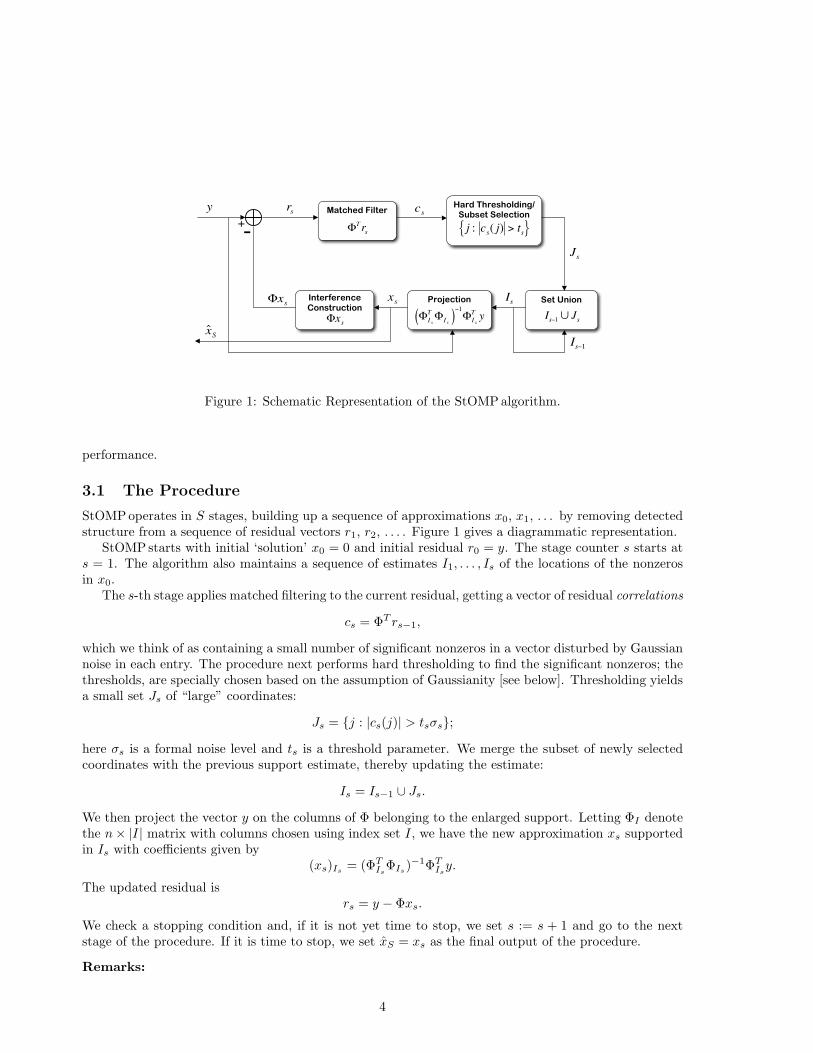
Figure 1: Schematic Representation of the StOMP algorithm.

performance.

3.1 The Procedure

StOMPoperates in S stages, building up a sequence of approximations x0, x1, . . . by removing detectedstructure from a sequence of residual vectors r1, r2, . . . . Figure 1 gives a diagrammatic representation.

StOMPstarts with initial ‘solution’ x0 = 0 and initial residual r0 = y. The stage counter s starts ats = 1. The algorithm also maintains a sequence of estimates I1, . . . , Is of the locations of the nonzerosin x0.

The s-th stage applies matched filtering to the current residual, getting a vector of residual correlations

cs = ΦT rs−1,

which we think of as containing a small number of significant nonzeros in a vector disturbed by Gaussiannoise in each entry. The procedure next performs hard thresholding to find the significant nonzeros; thethresholds, are specially chosen based on the assumption of Gaussianity [see below]. Thresholding yieldsa small set Js of “large” coordinates:

Js = {j : |cs(j)| > tsσs};

here σs is a formal noise level and ts is a threshold parameter. We merge the subset of newly selectedcoordinates with the previous support estimate, thereby updating the estimate:

Is = Is−1 ∪ Js.

We then project the vector y on the columns of Φ belonging to the enlarged support. Letting ΦI denotethe n× |I| matrix with columns chosen using index set I, we have the new approximation xs supportedin Is with coefficients given by

(xs)Is= (ΦT

IsΦIs

)−1ΦTIsy.

The updated residual isrs = y − Φxs.

We check a stopping condition and, if it is not yet time to stop, we set s := s + 1 and go to the nextstage of the procedure. If it is time to stop, we set xS = xs as the final output of the procedure.

Remarks:

4

1. The procedure resembles Orthogonal Matching Pursuit (known to statisticians as Forward StepwiseRegression). In fact the two would give identical results if S were equal to n and if, by coincidence,the threshold ts were set in such a way that a single new term were obtained in Js at each stage.

2. The thresholding strategy used in StOMP(to be described below) aims to have numerous termsenter at each stage, and aims to have a fixed number of stages. Hence the results will be differentfrom OMP.

3. The formal noise level σs = ‖rs‖2/√n, and typically the threshold parameter takes values in the

range 2 ≤ ts ≤ 3.

4. There are strong connections to: stagewise/stepwise regression in statistical model building; succes-sive interference cancellation multiuser detectors in digital communications and iterative decodersin error-control coding. See the discussion in Section 11.

Our recommended choice of S (10) and our recommended threshold-setting procedures (see Section3.4 below) have been designed so that when x0 is sufficiently sparse, the following two conditions arelikely to hold upon termination:

• All nonzeros in x0 are selected in IS .

• IS has no more than n entries.

The next lemma motivates this design criterion. Recall that Φ is sampled from the USE and socolumns of Φ are in general position. The following is proved in Appendix A.

Lemma 3.1 Let the columns of Φ be in general position. Let IS denote the support of xS. Suppose thatthe support I0 of x0 is a subset of IS. Suppose in addition that #IS ≤ n. Then we have perfect recovery:

xS = x0. (3.1)

3.2 An Example

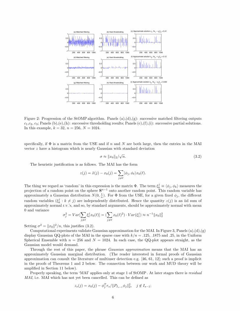
We give a simple example showing that the procedure works in a special case.We generated a coefficient vector x0 with k = 32 nonzeros, having amplitudes uniformly distributed

on [0, 1]. We sampled a matrix Φ at random from the USE with n = 256, N = 1024, and computed alinear measurement vector y = Φx0. Thus the problem of recovering x0 given y is 1 : 4 underdetermined(i.e. δ = n/N = .25), with underlying sparsity measure ρ = k/n = .125. To this SSP, we appliedStOMPcoupled with the CFAR threshold selection rule to be discussed below. The results are illustratedin Figure 2.

Panels (a)-(i) depict each matched filtering output, its hard thresholding and the evolving approxi-mation. As can be seen, after 3 stages a result is obtained which is quite sparse and, as the final panelshows, matches well the object x0 which truly generated the data. In fact, the error at the end of thethird stage measures ‖x3−x0‖2/‖x0‖2 = 0.022, i.e. a mere 3 stages were required to achieve an accuracyof 2 decimal digits.

3.3 Approximate Gaussianity of Residual MAI

At the heart of our procedure are two thresholding schemes often used in Gaussian noise removal. (N.B.at this point we assume there is no noise in y!) To explain the relevance of Gaussian ‘noise’ concepts,note that at stage 1, the algorithm is computing

x = ΦT y;

this is essentially the usual matched filter estimate of x0. If y = Φx0 and x0 vanishes except in onecoordinate, the matched filter output x equals x0 perfectly. Hence z = x − x0 is a measure of thedisturbance to exact reconstruction caused by multiple nonzeros in x0. The same notion arises in digitalcommunications where it is called Multiple-Access Interference (MAI) [60]. Perhaps surprisingly - becausethere is no noise in the problem - the MAI in our setting typically has a Gaussian behavior. More

5

200 400 600 800 1000−1

−0.5

0

0.5

1(a) Matched filtering

200 400 600 800 1000−1

−0.5

0

0.5

1(b) Hard thresholding

200 400 600 800 1000−1

−0.5

0

0.5

1

(c) Approximate solution x1, ||x

1 − x

0||

2 = 0.41

200 400 600 800 1000−1

−0.5

0

0.5

1(d) Matched filtering

200 400 600 800 1000−1

−0.5

0

0.5

1(e) Hard thresholding

200 400 600 800 1000−1

−0.5

0

0.5

1

(f) Approximate solution x2, ||x

2 − x

0||

2 = 0.12

200 400 600 800 1000−1

−0.5

0

0.5

1(g) Matched filtering

200 400 600 800 1000−1

−0.5

0

0.5

1(h) Hard thresholding

200 400 600 800 1000−1

−0.5

0

0.5

1

(i) Approximate solution x3, ||x

3 − x

0||

2 = 0.022

Figure 2: Progression of the StOMPalgorithm. Panels (a),(d),(g): successive matched filtering outputsc1,c2, c3; Panels (b),(e),(h): successive thresholding results; Panels (c),(f),(i): successive partial solutions.In this example, k = 32, n = 256, N = 1024.

specifically, if Φ is a matrix from the USE and if n and N are both large, then the entries in the MAIvector z have a histogram which is nearly Gaussian with standard deviation

σ ≈ ‖x0‖2/√n. (3.2)

The heuristic justification is as follows. The MAI has the form

z(j) = x(j)− x0(j) =∑j 6=`

〈φj , φ`〉x0(`).

The thing we regard as ‘random’ in this expression is the matrix Φ. The term ξjk ≡ 〈φj , φk〉 measures the

projection of a random point on the sphere Sn−1 onto another random point. This random variable hasapproximately a Gaussian distribution N(0, 1

n ). For Φ from the USE, for a given fixed φj , the differentrandom variables (ξj

k : k 6= j) are independently distributed. Hence the quantity z(j) is an iid sum ofapproximately normal r.v.’s, and so, by standard arguments, should be approximately normal with mean0 and variance

σ2j = V ar[

∑j 6=`

ξj`x0(`)] = (

∑j 6=`

x0(`)2) · V ar(ξj1) ≈ n−1‖x0‖2

2

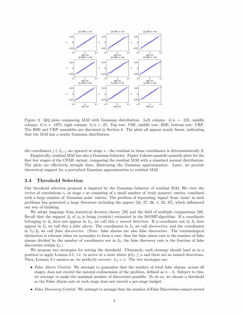
Setting σ2 = ‖x0‖2/n, this justifies (3.2).Computational experiments validate Gaussian approximation for the MAI. In Figure 3, Panels (a),(d),(g)

display Gaussian QQ-plots of the MAI in the sparse case with k/n = .125, .1875 and .25, in the UniformSpherical Ensemble with n = 256 and N = 1024. In each case, the QQ-plot appears straight, as theGaussian model would demand.

Through the rest of this paper, the phrase Gaussian approximation means that the MAI has anapproximately Gaussian marginal distribution. (The reader interested in formal proofs of Gaussianapproximation can consult the literature of multiuser detection e.g. [46, 61, 12]; such a proof is implicitin the proofs of Theorems 1 and 2 below. The connection between our work and MUD theory will beamplified in Section 11 below).

Properly speaking, the term ‘MAI’ applies only at stage 1 of StOMP . At later stages there is residualMAI, i.e. MAI which has not yet been cancelled. This can be defined as

zs(j) = x0(j)− φTj rs/‖PIs−1φj‖2

2, j 6∈ Is−1;

6

−0.1 0 0.1

−0.01

0

0.01

N(0,1/n)

z

(a) USE, k = 32

−0.1 0 0.1

−0.01

0

0.01

N(0,1/n)

z

(d) USE, k = 32

−0.1 0 0.1

−0.01

0

0.01

N(0,1/n)

z

(g) USE, k = 32

−0.1 0 0.1

−0.01

0

0.01

N(0,1/n)

z

(b) RSE, k = 48

−0.1 0 0.1

−0.01

0

0.01

N(0,1/n)

z

(e) RSE, k = 48

−0.1 0 0.1

−0.01

0

0.01

N(0,1/n)

z

(h) RSE, k = 48

−0.1 0 0.1

−0.01

0

0.01

N(0,1/n)

z

(c) URP, k = 64

−0.1 0 0.1

−0.01

0

0.01

N(0,1/n)

z

(f) URP, k = 64

−0.1 0 0.1

−0.01

0

0.01

N(0,1/n)

z

(i) URP, k = 64

Figure 3: QQ plots comparing MAI with Gaussian distribution. Left column: k/n = .125, middlecolumn: k/n = .1875, right column: k/n = .25. Top row: USE, middle row: RSE, bottom row: URP.The RSE and URP ensembles are discussed in Section 8. The plots all appear nearly linear, indicatingthat the MAI has a nearly Gaussian distribution.

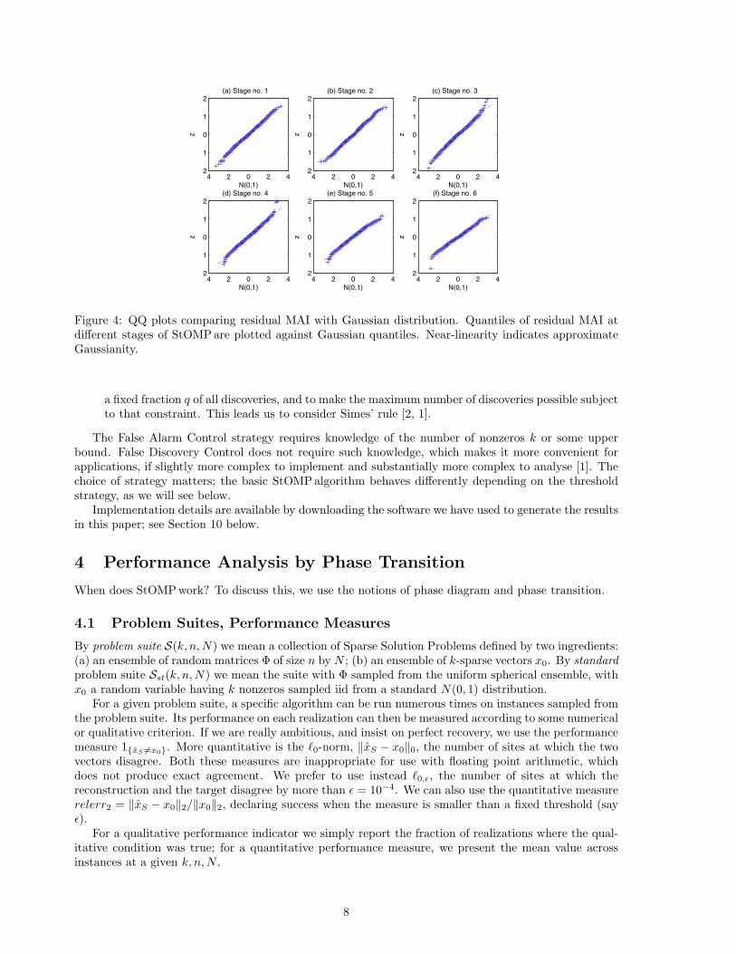
the coordinates j ∈ Is−1 are ignored at stage s - the residual in those coordinates is deterministically 0.Empirically, residual MAI has also a Gaussian behavior. Figure 4 shows quantile-quantile plots for the

first few stages of the CFAR variant, comparing the residual MAI with a standard normal distribution.The plots are effectively straight lines, illustrating the Gaussian approximation. Later, we providetheoretical support for a perturbed Gaussian approximation to residual MAI.

3.4 Threshold Selection

Our threshold selection proposal is inspired by the Gaussian behavior of residual MAI. We view thevector of correlations cs at stage s as consisting of a small number of ‘truly nonzero’ entries, combinedwith a large number of ‘Gaussian noise’ entries. The problem of separating ‘signal’ from ‘noise’ in suchproblems has generated a large literature including the papers [24, 27, 26, 1, 23, 37], which influencedour way of thinking.

We adopt language from statistical decision theory [39] and the field of multiple comparisons [38].Recall that the support I0 of x0 is being (crudely) estimated in the StOMPalgorithm. If a coordinatebelonging to I0 does not appear in IS , we call this a missed detection. If a coordinate not in I0 doesappear in IS we call this a false alarm. The coordinates in IS we call discoveries, and the coordinatesin IS\I0 we call false discoveries. (Note: false alarms are also false discoveries. The terminologicaldistinction is relevant when we normalize to form a rate; thus the false alarm rate is the number of falsealarms divided by the number of coordinates not in I0; the false discovery rate is the fraction of falsediscoveries within IS .)

We propose two strategies for setting the threshold. Ultimately, each strategy should land us in aposition to apply Lemma 3.1: i.e. to arrive at a state where #IS ≤ n and there are no missed detections.Then, Lemma 3.1 assures us, we perfectly recover: xS = x. The two strategies are:

• False Alarm Control. We attempt to guarantee that the number of total false alarms, across allstages, does not exceed the natural codimension of the problem, defined as n− k. Subject to this,we attempt to make the maximal number of discoveries possible. To do so, we choose a thresholdso the False Alarm rate at each stage does not exceed a per-stage budget.

• False Discovery Control. We attempt to arrange that the number of False Discoveries cannot exceed

7

4 2 0 2 42

1

0

1

2

N(0,1)z

(a) Stage no. 1

4 2 0 2 42

1

0

1

2

N(0,1)

z

(b) Stage no. 2

4 2 0 2 42

1

0

1

2

N(0,1)

z

(c) Stage no. 3

4 2 0 2 42

1

0

1

2

N(0,1)

z(d) Stage no. 4

4 2 0 2 42

1

0

1

2

N(0,1)z

(e) Stage no. 5

4 2 0 2 42

1

0

1

2

N(0,1)

z

(f) Stage no. 6

Figure 4: QQ plots comparing residual MAI with Gaussian distribution. Quantiles of residual MAI atdifferent stages of StOMPare plotted against Gaussian quantiles. Near-linearity indicates approximateGaussianity.

a fixed fraction q of all discoveries, and to make the maximum number of discoveries possible subjectto that constraint. This leads us to consider Simes’ rule [2, 1].

The False Alarm Control strategy requires knowledge of the number of nonzeros k or some upperbound. False Discovery Control does not require such knowledge, which makes it more convenient forapplications, if slightly more complex to implement and substantially more complex to analyse [1]. Thechoice of strategy matters; the basic StOMPalgorithm behaves differently depending on the thresholdstrategy, as we will see below.

Implementation details are available by downloading the software we have used to generate the resultsin this paper; see Section 10 below.

4 Performance Analysis by Phase Transition

When does StOMPwork? To discuss this, we use the notions of phase diagram and phase transition.

4.1 Problem Suites, Performance Measures

By problem suite S(k, n,N) we mean a collection of Sparse Solution Problems defined by two ingredients:(a) an ensemble of random matrices Φ of size n by N ; (b) an ensemble of k-sparse vectors x0. By standardproblem suite Sst(k, n,N) we mean the suite with Φ sampled from the uniform spherical ensemble, withx0 a random variable having k nonzeros sampled iid from a standard N(0, 1) distribution.

For a given problem suite, a specific algorithm can be run numerous times on instances sampled fromthe problem suite. Its performance on each realization can then be measured according to some numericalor qualitative criterion. If we are really ambitious, and insist on perfect recovery, we use the performancemeasure 1{xS 6=x0}. More quantitative is the `0-norm, ‖xS − x0‖0, the number of sites at which the twovectors disagree. Both these measures are inappropriate for use with floating point arithmetic, whichdoes not produce exact agreement. We prefer to use instead `0,ε, the number of sites at which thereconstruction and the target disagree by more than ε = 10−4. We can also use the quantitative measurerelerr2 = ‖xS − x0‖2/‖x0‖2, declaring success when the measure is smaller than a fixed threshold (sayε).

For a qualitative performance indicator we simply report the fraction of realizations where the qual-itative condition was true; for a quantitative performance measure, we present the mean value acrossinstances at a given k, n,N .

8

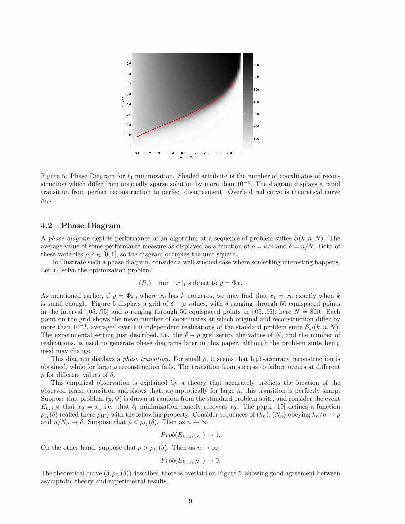
Figure 5: Phase Diagram for `1 minimization. Shaded attribute is the number of coordinates of recon-struction which differ from optimally sparse solution by more than 10−4. The diagram displays a rapidtransition from perfect reconstruction to perfect disagreement. Overlaid red curve is theoretical curveρ`1 .

4.2 Phase Diagram

A phase diagram depicts performance of an algorithm at a sequence of problem suites S(k, n,N). Theaverage value of some performance measure as displayed as a function of ρ = k/n and δ = n/N . Both ofthese variables ρ, δ ∈ [0, 1], so the diagram occupies the unit square.

To illustrate such a phase diagram, consider a well-studied case where something interesting happens.Let x1 solve the optimization problem:

(P1) min ‖x‖1 subject to y = Φx.

As mentioned earlier, if y = Φx0 where x0 has k nonzeros, we may find that x1 = x0 exactly when kis small enough. Figure 5 displays a grid of δ − ρ values, with δ ranging through 50 equispaced pointsin the interval [.05, .95] and ρ ranging through 50 equispaced points in [.05, .95]; here N = 800. Eachpoint on the grid shows the mean number of coordinates at which original and reconstruction differ bymore than 10−4, averaged over 100 independent realizations of the standard problem suite Sst(k, n,N).The experimental setting just described, i.e. the δ − ρ grid setup, the values of N , and the number ofrealizations, is used to generate phase diagrams later in this paper, although the problem suite beingused may change.

This diagram displays a phase transition. For small ρ, it seems that high-accuracy reconstruction isobtained, while for large ρ reconstruction fails. The transition from success to failure occurs at differentρ for different values of δ.

This empirical observation is explained by a theory that accurately predicts the location of theobserved phase transition and shows that, asymptotically for large n, this transition is perfectly sharp.Suppose that problem (y,Φ) is drawn at random from the standard problem suite, and consider the eventEk,n,N that x0 = x1 i.e. that `1 minimization exactly recovers x0. The paper [19] defines a functionρ`1(δ) (called there ρW ) with the following property. Consider sequences of (kn), (Nn) obeying kn/n→ ρand n/Nn → δ. Suppose that ρ < ρ`1(δ). Then as n→∞

Prob(Ekn,n,Nn) → 1.

On the other hand, suppose that ρ > ρ`1(δ). Then as n→∞

Prob(Ekn,n,Nn) → 0.

The theoretical curve (δ, ρ`1(δ)) described there is overlaid on Figure 5, showing good agreement betweenasymptotic theory and experimental results.

9

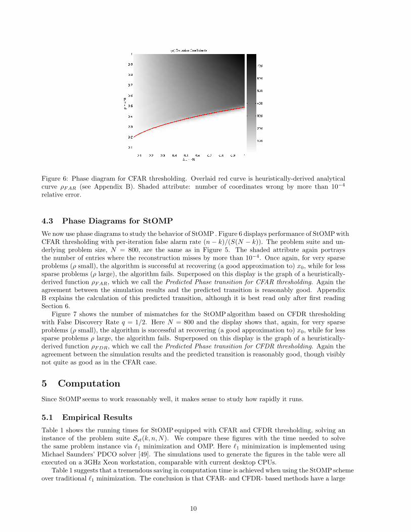
Figure 6: Phase diagram for CFAR thresholding. Overlaid red curve is heuristically-derived analyticalcurve ρFAR (see Appendix B). Shaded attribute: number of coordinates wrong by more than 10−4

relative error.

4.3 Phase Diagrams for StOMP

We now use phase diagrams to study the behavior of StOMP . Figure 6 displays performance of StOMPwithCFAR thresholding with per-iteration false alarm rate (n− k)/(S(N − k)). The problem suite and un-derlying problem size, N = 800, are the same as in Figure 5. The shaded attribute again portraysthe number of entries where the reconstruction misses by more than 10−4. Once again, for very sparseproblems (ρ small), the algorithm is successful at recovering (a good approximation to) x0, while for lesssparse problems (ρ large), the algorithm fails. Superposed on this display is the graph of a heuristically-derived function ρFAR, which we call the Predicted Phase transition for CFAR thresholding. Again theagreement between the simulation results and the predicted transition is reasonably good. AppendixB explains the calculation of this predicted transition, although it is best read only after first readingSection 6.

Figure 7 shows the number of mismatches for the StOMPalgorithm based on CFDR thresholdingwith False Discovery Rate q = 1/2. Here N = 800 and the display shows that, again, for very sparseproblems (ρ small), the algorithm is successful at recovering (a good approximation to) x0, while for lesssparse problems ρ large, the algorithm fails. Superposed on this display is the graph of a heuristically-derived function ρFDR, which we call the Predicted Phase transition for CFDR thresholding. Again theagreement between the simulation results and the predicted transition is reasonably good, though visiblynot quite as good as in the CFAR case.

5 Computation

Since StOMPseems to work reasonably well, it makes sense to study how rapidly it runs.

5.1 Empirical Results

Table 1 shows the running times for StOMP equipped with CFAR and CFDR thresholding, solving aninstance of the problem suite Sst(k, n,N). We compare these figures with the time needed to solvethe same problem instance via `1 minimization and OMP. Here `1 minimization is implemented usingMichael Saunders’ PDCO solver [49]. The simulations used to generate the figures in the table were allexecuted on a 3GHz Xeon workstation, comparable with current desktop CPUs.

Table 1 suggests that a tremendous saving in computation time is achieved when using the StOMPschemeover traditional `1 minimization. The conclusion is that CFAR- and CFDR- based methods have a large

10

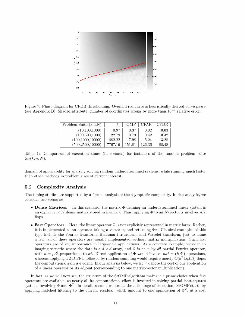
Figure 7: Phase diagram for CFDR thresholding. Overlaid red curve is heuristically-derived curve ρFDR

(see Appendix B). Shaded attribute: number of coordinates wrong by more than 10−4 relative error.

Problem Suite (k,n,N) `1 OMP CFAR CFDR(10,100,1000) 0.97 0.37 0.02 0.03

(100,500,1000) 22.79 0.79 0.42 0.32(100,1000,10000) 482.22 7.98 5.24 3.28(500,2500,10000) 7767.16 151.81 126.36 88.48

Table 1: Comparison of execution times (in seconds) for instances of the random problem suiteSst(k, n,N).

domain of applicability for sparsely solving random underdetermined systems, while running much fasterthan other methods in problem sizes of current interest.

5.2 Complexity Analysis

The timing studies are supported by a formal analysis of the asymptotic complexity. In this analysis, weconsider two scenarios.

• Dense Matrices. In this scenario, the matrix Φ defining an underdetermined linear system isan explicit n×N dense matrix stored in memory. Thus, applying Φ to an N -vector x involves nNflops.

• Fast Operators. Here, the linear operator Φ is not explicitly represented in matrix form. Rather,it is implemented as an operator taking a vector x, and returning Φx. Classical examples of thistype include the Fourier transform, Hadamard transform, and Wavelet transform, just to namea few; all of these operators are usually implemented without matrix multiplication. Such fastoperators are of key importance in large-scale applications. As a concrete example, consider animaging scenario where the data is a d × d array, and Φ is an n by d2 partial Fourier operator,with n = µd2 proportional to d2. Direct application of Φ would involve nd2 = O(d4) operations,whereas applying a 2-D FFT followed by random sampling would require merely O(d2 log(d)) flops;the computational gain is evident. In our analysis below, we let V denote the cost of one applicationof a linear operator or its adjoint (corresponding to one matrix-vector multiplication).

In fact, as we will now see, the structure of the StOMPalgorithm makes it a prime choice when fastoperators are available, as nearly all its computational effort is invested in solving partial least-squaressystems involving Φ and ΦT . In detail, assume we are at the s-th stage of execution. StOMP starts byapplying matched filtering to the current residual, which amount to one application of ΦT , at a cost

11

of nN flops. Next, it applies hard-thresholding to the residual correlations and updates the active setaccordingly, using at most 2N additional flops. The core of the computation lies in calculating theprojection of y onto the subset of columns ΦIs , to get a new approximation xs. This is implemented viaa Conjugate Gradient (CG) solver [34]. Each CG iteration involves application of ΦIs

and ΦTIs

, costingat most 2nN + O(N) flops. The number of CG iterations used is a small constant, independent of nand N , which we denote ν. In our implementation we use ν = 10. Finally, we compute the new residualby applying Φ to the new approximation, requiring an additional nN flops. Summarizing, the totaloperation count per StOMPstage amounts to (ν + 2)nN + O(N). The total number of StOMPstages,S, is a prescribed constant, independent of the data; in the simulations in this paper we set S = 10.

Readers familiar with OMP have by now doubtless recognized the evident parallelism in the algorith-mic structure of StOMPand OMP. Indeed, much like StOMP , at each stage OMP computes residualcorrelations and solves a least-squares problem for the new solution estimate. Yet, unlike StOMP , OMPbuilds up the active set one element at a time. Hence, an efficient implementation would necessarily main-tain a Cholesky factorization of the active set matrix and update it at each stage, thereby reducing thecost of solving the least-squares system. In total, k steps of OMP would take at most 4k3/3+knN+O(N)flops. Without any sparsity assumptions on the data, OMP takes at most n steps, thus, its worst-caseperformance is bounded by 4n3/3+n2N+O(N) operations. A key difference between StOMP and OMPis that the latter needs to store the Cholesky factor of the active set matrix in its explicit form, takingup to n2/2 memory elements. When n is large, as is often the case in 2- and 3-D image-reconstructionscenarios, this greatly hinders the applicability of OMP. In contrast, StOMP has very modest storagerequirements. At any given point of the algorithm execution, one needs only store the current estimatexs, the current residual vector rs, and the current active set Is. This makes StOMPvery attractive foruse in large-scale applications.

Table 2 summarizes our discussion so far, offering a comparison of the computational complexity ofStOMP , OMP and `1 minimization via linear programming (LP). For the LP solver, we use a primal-dual barrier method for convex optimization (PDCO) developed by Michael Saunders [49]. The estimateslisted in the table all assume worst-case behavior. Examining the bounds in the dense matrix case closely,we notice that StOMP is the only algorithm of the three admitting quadratic order complexity estimates.In contrast, OMP and PDCO require cubic order estimates for their worst-case performance bound.Therefore, for large scale problems StOMP can dominate due to its simple structure and efficiency. Inthe case where fast operators are applicable, StOMPyet again prevails; it is the only algorithm of thethree requiring a constant number (S · (ν + 2)) of matrix-vector multiplications to reach a solution.

Algorithm Dense Matrices Fast OperatorsStOMP S(ν + 2)nN +O(N) S(ν + 2) · V +O(N)OMP 4n3/3 + n2N +O(N) 4n3/3 + 2n · V +O(N)`1 min. with PDCO S(2N)3/3 +O(nN) 2N · V +O(nN)

Table 2: Worst-Case Complexity Bounds for StOMP , OMP and PDCO. S denotes the maximum numberof stages, ν denotes the maximum number of CG iterations employed per stage of StOMP, and V standsfor the cost of one matrix-vector product (implemented as a fast operator).

To convey the scale of computational benefits in large problems, we conduct a simple experiment ina setting where Φ can be implemented as a fast operator. We consider a system y = Φx where Φ ismade from only n = δN rows of the Fourier matrix. Φ can be implemented by application of a FastFourier Transform followed by a coordinate selection. Table 3 gives the results. Clearly the advantageof StOMP is even more convincing.

Problem Suite (k,n,N) `1 OMP CFAR CFDRSPFE (500,10000,20000) 237.69 53.64 2.07 3.16SPFE (1000,20000,50000) 810.39 299.54 5.63 9.47

Table 3: Comparison of execution times (in seconds) in the random partial Fourier suite SPFE(k, n,N).Because of the fast operator, StOMPoutperforms OMP.

12

0.1 0.15 0.2 0.25 0.3 0.35 0.4 0.450

0.1

0.2

0.3

0.4

0.5

0.6

0.7

0.8

0.9

1Early Terminations

δ

Pro

babi

lity

of E

arly

Ter

min

atio

n

n = 400n=800n=1600

0.1 0.15 0.2 0.25 0.3 0.35 0.4 0.450

0.1

0.2

0.3

0.4

0.5

0.6

0.7Missed Detections

δ

Fra

ctio

n T

ruly

Non

Nul

l Mis

sed

n = 400n=800n=1600

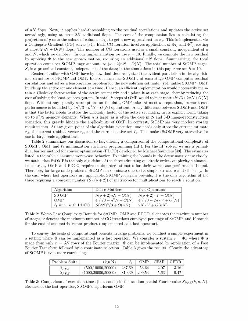
Figure 8: Empirical Transition Behaviors, varying n. (a) Fraction of cases with termination before stageS. (b) Fraction of missed detections. Averages of 1000 trials with n = 400, 800, 1600 and k = bρnc,N = bn/δc, δ = 1/4 and ρ varying. Sharpness of each transition seems to be increasing with n.

To make the comparison still more vivid, we point ahead to an imaging example from Section 9.1below. There an image of dimensions d× d is viewed as a vector x of length N = d2. Again the systemy = Φx where Φ is made from only n = δN rows of the Fourier matrix. One matrix-vector product costsV = 4N logN = 8d2 log d.

How do the three algorithms compare in this setting? Plugging-in S = 10, ν = 10, and V as above, wesee that the leading term in the complexity bound for StOMP is 960 · d2 log d. In contrast, for OMP theleading term in the worst-case bound becomes 4δ3

3 d6 + 16δd4 log d, and for `1 minimization the leadingterm is 16d4 log d. The computational gains from StOMP are indeed substantial. Moreover, to run OMPin this setting, we may need up to δ2

2 d4 memory elements to store the Cholesky factorization, which

renders it unusable for anything but the smallest d. In Section 9.1, we present actual running times ofthe different algorithms.

6 The Large-System Limit

Figures 6 and 7 suggest phase transitions in the behavior of StOMP , which would imply a certainwell-defined asymptotic ‘system capacity’ below which StOMPsuccessfully finds a sparse solution, andabove which it fails. In this section, we review the empirical evidence for a phase transition in thelarge-system limit and develop theory that rigorously establishes it. We consider the problem suiteS(k, n,N ;USE,±1) defined by random Φ sampled from the USE, and with y generated as y = Φx0,where x0 has k nonzero coefficients in random positions having entries ±1. This ensemble generates aslightly ‘lower’ transition than the ensemble used for Figures 6 and 7 where the nonzeros in x0 had iidGaussian N(0, 1) entries.

6.1 Evidence for Phase Transition

Figure 8 presents results of simulations at fixed ratios δ = n/N but increasing n. Three differentquantities are considered: in panel (a), the probability of early termination, i.e. termination before stageS = 10 because the residual has been driven nearly to zero; in panel (b) the missed detection rate, i.e.the fraction of nonzeros in x0 that are not supported in the reconstruction xS . Both quantities undergotransitions in behavior near ρ = .2.

Significantly, the transitions become more sharply defined with increasing n. As n increases, theearly termination probability behaves increasingly like a raw discontinuity 1{k/n≥ρF AR(n/N)} as n→∞,while the fraction of missed detections properties behave increasingly like a discontinuity in derivative(k/n−ρFAR(n/N))+. In statistical physics such limiting behaviors are called first-order and second-orderphase transitions, respectively.

13

(k, n, N) ρ1 ρ2 ρ3 ρ4 d1 d2 d3 d4 ν1 ν2 ν3 ν4(70,280,800) 0.250 0.130 0.074 0.041 1.000 0.773 0.630 0.521 2.857 2.630 2.487 2.377

(105,420,1200) 0.250 0.130 0.075 0.043 1.000 0.775 0.633 0.524 2.857 2.632 2.490 2.381(140,560,1600) 0.250 0.131 0.075 0.043 1.000 0.776 0.632 0.522 2.857 2.633 2.489 2.379(210,840,2400) 0.250 0.130 0.075 0.043 1.000 0.776 0.630 0.522 2.856 2.632 2.486 2.378(78,280,800) 0.279 0.158 0.106 0.078 1.000 0.778 0.643 0.546 2.857 2.635 2.499 2.403

(117,420,1200) 0.279 0.157 0.104 0.073 1.000 0.781 0.646 0.546 2.857 2.638 2.502 2.403(156,560,1600) 0.279 0.159 0.105 0.076 1.000 0.782 0.645 0.545 2.857 2.639 2.502 2.401(235,840,2400) 0.280 0.159 0.106 0.076 1.000 0.778 0.644 0.542 2.856 2.635 2.501 2.399

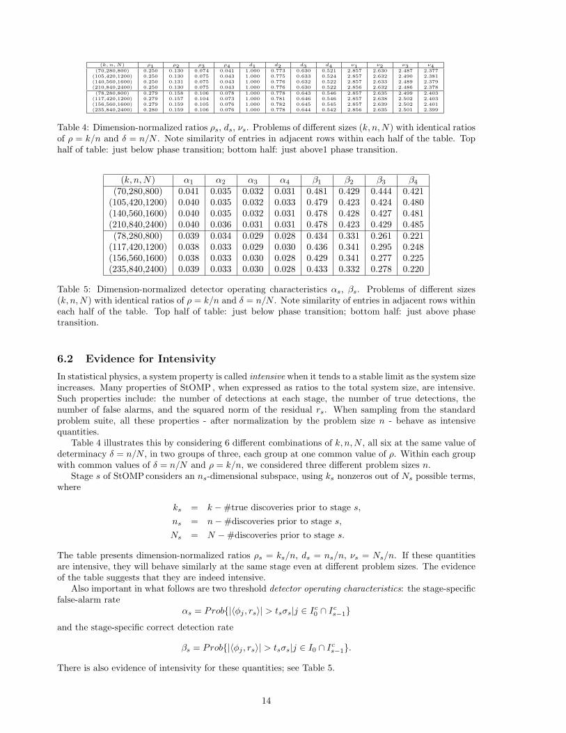
Table 4: Dimension-normalized ratios ρs, ds, νs. Problems of different sizes (k, n,N) with identical ratiosof ρ = k/n and δ = n/N . Note similarity of entries in adjacent rows within each half of the table. Tophalf of table: just below phase transition; bottom half: just above1 phase transition.

(k, n,N) α1 α2 α3 α4 β1 β2 β3 β4

(70,280,800) 0.041 0.035 0.032 0.031 0.481 0.429 0.444 0.421(105,420,1200) 0.040 0.035 0.032 0.033 0.479 0.423 0.424 0.480(140,560,1600) 0.040 0.035 0.032 0.031 0.478 0.428 0.427 0.481(210,840,2400) 0.040 0.036 0.031 0.031 0.478 0.423 0.429 0.485(78,280,800) 0.039 0.034 0.029 0.028 0.434 0.331 0.261 0.221

(117,420,1200) 0.038 0.033 0.029 0.030 0.436 0.341 0.295 0.248(156,560,1600) 0.038 0.033 0.030 0.028 0.429 0.341 0.277 0.225(235,840,2400) 0.039 0.033 0.030 0.028 0.433 0.332 0.278 0.220

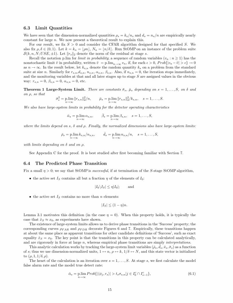
Table 5: Dimension-normalized detector operating characteristics αs, βs. Problems of different sizes(k, n,N) with identical ratios of ρ = k/n and δ = n/N . Note similarity of entries in adjacent rows withineach half of the table. Top half of table: just below phase transition; bottom half: just above phasetransition.

6.2 Evidence for Intensivity

In statistical physics, a system property is called intensive when it tends to a stable limit as the system sizeincreases. Many properties of StOMP , when expressed as ratios to the total system size, are intensive.Such properties include: the number of detections at each stage, the number of true detections, thenumber of false alarms, and the squared norm of the residual rs. When sampling from the standardproblem suite, all these properties - after normalization by the problem size n - behave as intensivequantities.

Table 4 illustrates this by considering 6 different combinations of k, n,N , all six at the same value ofdeterminacy δ = n/N , in two groups of three, each group at one common value of ρ. Within each groupwith common values of δ = n/N and ρ = k/n, we considered three different problem sizes n.

Stage s of StOMPconsiders an ns-dimensional subspace, using ks nonzeros out of Ns possible terms,where

ks = k −#true discoveries prior to stage s,ns = n−#discoveries prior to stage s,Ns = N −#discoveries prior to stage s.

The table presents dimension-normalized ratios ρs = ks/n, ds = ns/n, νs = Ns/n. If these quantitiesare intensive, they will behave similarly at the same stage even at different problem sizes. The evidenceof the table suggests that they are indeed intensive.

Also important in what follows are two threshold detector operating characteristics: the stage-specificfalse-alarm rate

αs = Prob{|〈φj , rs〉| > tsσs|j ∈ Ic0 ∩ Ic

s−1}

and the stage-specific correct detection rate

βs = Prob{|〈φj , rs〉| > tsσs|j ∈ I0 ∩ Ics−1}.

There is also evidence of intensivity for these quantities; see Table 5.

14

6.3 Limit Quantities

We have seen that the dimension-normalized quantities ρs = ks/ns and ds = ns/n are empirically nearlyconstant for large n. We now present a theoretical result to explain this.

For our result, we fix S > 0 and consider the CFAR algorithm designed for that specified S. Wealso fix ρ, δ ∈ (0, 1). Let k = kn = bρnc, Nn = bn/δc. Run StOMP on an instance of the problem suiteS(k, n,N ;USE,±1). Let ‖rs‖2 denote the norm of the residual at stage s.

Recall the notation p.lim for limit in probability; a sequence of random variables (vn : n ≥ 1) has thenonstochastic limit v in probability, written v = p.limn→∞ vn, if, for each ε > 0, Prob{|vn− v| > ε} → 0as n→∞. In the result below, let ks,n denote the random quantity ks on a problem from the standardsuite at size n. Similarly for rs,n,ds,n, ns,n, αs,n, βs,n. Also, if ns,n = 0, the iteration stops immediately,and the monitoring variables at that and all later stages up to stage S are assigned values in the obviousway: rs,n = 0, βs,n = 0, αs,n = 0, etc.

Theorem 1 Large-System Limit. There are constants σs, µs depending on s = 1, . . . , S, on δ andon ρ, so that

σ2s = p.lim

n→∞‖rs,n‖2

2/n, µs = p.limn→∞

‖rs,n‖22/ks,n, s = 1, . . . , S.

We also have large-system limits in probability for the detector operating characteristics

αs = p.limn→∞

αs,n, βs = p.limn→∞

βs,n, s = 1, . . . , S,

where the limits depend on s, δ and ρ. Finally, the normalized dimensions also have large-system limits:

ρs = p.limn→∞

ks,n/ns,n, ds = p.limn→∞

ns,n/n, s = 1, . . . , S,

with limits depending on δ and on ρ.

See Appendix C for the proof. It is best studied after first becoming familiar with Section 7.

6.4 The Predicted Phase Transition

Fix a small η > 0; we say that StOMP is successful, if at termination of the S-stage StOMPalgorithm,

• the active set IS contains all but a fraction η of the elements of I0:

|I0\IS | ≤ η|I0|; and

• the active set IS contains no more than n elements:

|IS | ≤ (1− η)n.

Lemma 3.1 motivates this definition (in the case η = 0). When this property holds, it is typically thecase that xS ≈ x0, as experiments have shown.

The existence of large-system limits allows us to derive phase transitions in the ‘Success’ property; thecorresponding curves ρFAR and ρFDR decorate Figures 6 and 7. Empirically, these transitions happenat about the same place as apparent transitions for other candidate definitions of ‘Success’, such as exactequality xS = x0. The key point is that the transitions in this property can be calculated analytically,and are rigorously in force at large n, whereas empirical phase transitions are simply interpretations.

This analytic calculation works by tracking the large-system limit variables (ρs, ds, νs, σs) as a functionof s; thus we use dimension-normalized units, 1 ↔ n, ρ↔ k, 1/δ ↔ N , and this state vector is initializedto (ρ, 1, 1/δ, ρ).

The heart of the calculation is an iteration over s = 1, . . . , S. At stage s, we first calculate the modelfalse alarm rate and the model true detect rate:

αs = p.limn→∞

Prob{|〈φj , rs〉| > tsσs,n|j ∈ Ic0 ∩ Ic

s−1}, (6.1)

15

Method δ = .05 δ = .10 .15 .20 .25 .35 .50 .65 .80Empirical 0.1250 0.1562 0.1792 0.2000 0.2225 0.2607 0.3212 0.3663 0.3852

Theoretical 0.1247 0.1498 0.1703 0.1869 0.2076 0.2518 0.2913 0.3567 0.4008

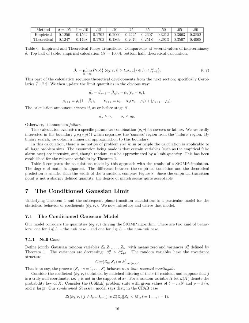
Table 6: Empirical and Theoretical Phase Transitions. Comparisons at several values of indeterminacyδ. Top half of table: empirical calculation (N = 1600); bottom half: theoretical calculation.

βs = p.limn→∞

Prob{|〈φj , rs〉| > tsσs,n|j ∈ I0 ∩ Ics−1}. (6.2)

This part of the calculation requires theoretical developments from the next section; specifically Corol-laries 7.1,7.2. We then update the limit quantities in the obvious way:

ds = ds−1 − βsρs − αs(νs − ρs),

ρs+1 = ρs(1− βs), νs+1 = νs − αs(νs − ρs) + (ρs+1 − ρs).

The calculation announces success if, at or before stage S,

ds ≥ η, ρs ≤ ηρ.

Otherwise, it announces failure.This calculation evaluates a specific parameter combination (δ, ρ) for success or failure. We are really

interested in the boundary ρFAR,S(δ) which separates the ‘success’ region from the ‘failure’ region. Bybinary search, we obtain a numerical approximation to this boundary.

In this calculation, there is no notion of problem size n; in principle the calculation is applicable toall large problem sizes. The assumption being made is that certain variables (such as the empirical falsealarm rate) are intensive, and, though random, can be approximated by a limit quantity. This has beenestablished for the relevant variables by Theorem 1.

Table 6 compares the calculations made by this approach with the results of a StOMPsimulation.The degree of match is apparent. The difference between the empirical transition and the theoreticalprediction is smaller than the width of the transition; compare Figure 8. Since the empirical transitionpoint is not a sharply defined quantity, the degree of match seems quite acceptable.

7 The Conditioned Gaussian Limit

Underlying Theorem 1 and the subsequent phase-transition calculations is a particular model for thestatistical behavior of coefficients 〈φj , rs〉. We now introduce and derive that model.

7.1 The Conditioned Gaussian Model

Our model considers the quantities 〈φj , rs〉 driving the StOMPalgorithm. There are two kind of behav-iors: one for j 6∈ I0 – the null case – and one for j ∈ I0 – the non-null case.

7.1.1 Null Case

Define jointly Gaussian random variables Z0,Z1,. . . , ZS , with means zero and variances σ2s defined by

Theorem 1. The variances are decreasing: σ2s > σ2

s+1. The random variables have the covariancestructure

Cov(Zu, Zs) = σ2max(u,s).

That is to say, the process (Zs : s = 1, . . . , S) behaves as a time-reversed martingale.Consider the coefficient 〈φj , rs〉 obtained by matched filtering of the s-th residual, and suppose that j

is a truly null coordinate, i.e. j is not in the support of x0. For a random variable X let L(X) denote theprobability law of X. Consider the (USE,±) problem suite with given values of δ = n/N and ρ = k/n,and n large. Our conditioned Gaussian model says that, in the CFAR case

L(〈φj , rs〉|j 6∈ I0 ∪ Is−1) ≈ L(Zs||Zi| < tσi, i = 1, ..., s− 1).

16

In words, we model each null coefficient as a certain Gaussian random variable conditioned on certainnon-exceedance events involving other, correlated random variables. In particular, we do not model itsimply as a Gaussian random variable (except if s = 1). To enforce this distinction, we let Zs denote therandom variable Zs conditioned on {|Zi| < tσi, i = 1, ..., s− 1}.

7.1.2 Non-Null Case

Define jointly Gaussian random variables X0,X1,...,XS , with means µs and variances σ2s again deriving

from Theorem 1. There is again the covariance appropriate to a time-reversed martingale:

Cov(Xu, Xs) = σ2max(u,s).

Consider now the coefficient 〈φj , rs〉 obtained by matched filtering of the s-th residual, where j is atruly non-null coordinate, i.e. j is not in the support of x0. Consider again the standard problem suitewith given values of δ and ρ and n large. The conditioned Gaussian model says that

L(〈φj , rs〉|j ∈ I0 ∩ Ics−1) ≈ L(Xs||Xi| < tσi, i = 1, ..., s− 1).

In words, we model each non-null coefficient at stage s as a certain nonzero-mean Gaussian randomvariable conditioned on a certain sequence of non-exceedances at earlier stages in the sequence. In thiscase, the conditioning event looks the same as in the non-null case; however the random variables Xi donot have mean zero. We let Xs denote the random variableXs conditioned on {|Xi| < tσi, i = 1, ..., s−1}.

7.1.3 The Gaussian Approximation

The CG model, which will later be seen to be highly accurate, explains why the Gaussian approximationsometimes works. The model has the following consequence. Let pZs

(z) denote the marginal probabilitydensity of the CG variable Zs and let gσs

(z) denote the probability density of a Gaussian N(0, σ2s).

Under a simple normal approxmation, we would have pZs(z) ≈ gσs(z). Under our model,

ps(z) =Prob{|Z1| < tσ1, . . . , |Zs−1| < tσs−1|Zs = z}gσs(z)

Prob{|Z1| < tσ1, . . . , |Zs−1| < tσs−1}.

We have the identity pZs(z) = λs(z)gσs

(z), where

λs(z) =Prob{|Z1| < tσ1, . . . , |Zs−1| < tσs−1|Zs = z}

Prob{|Z1| < tσ1, . . . , |Zs−1| < tσs−1}.

A parallel definition for the random variables Xs sets

ξs(x) = pXs(x)/pXs

(x).

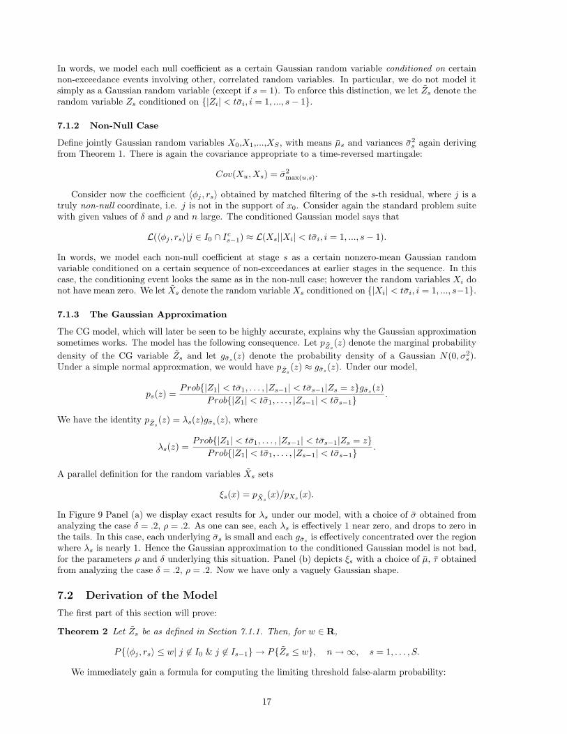
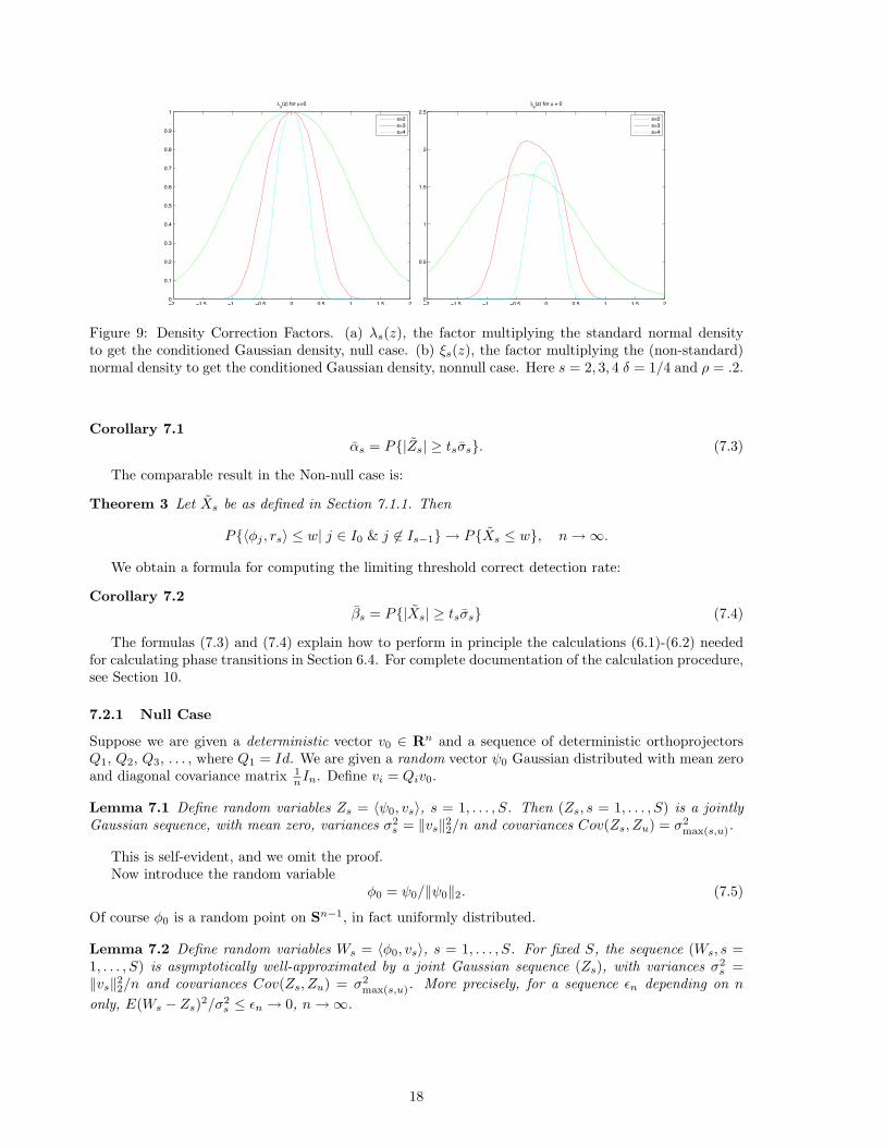
In Figure 9 Panel (a) we display exact results for λs under our model, with a choice of σ obtained fromanalyzing the case δ = .2, ρ = .2. As one can see, each λs is effectively 1 near zero, and drops to zero inthe tails. In this case, each underlying σs is small and each gσs

is effectively concentrated over the regionwhere λs is nearly 1. Hence the Gaussian approximation to the conditioned Gaussian model is not bad,for the parameters ρ and δ underlying this situation. Panel (b) depicts ξs with a choice of µ, τ obtainedfrom analyzing the case δ = .2, ρ = .2. Now we have only a vaguely Gaussian shape.

7.2 Derivation of the Model

The first part of this section will prove:

Theorem 2 Let Zs be as defined in Section 7.1.1. Then, for w ∈ R,

P{〈φj , rs〉 ≤ w| j 6∈ I0 & j 6∈ Is−1} → P{Zs ≤ w}, n→∞, s = 1, . . . , S.

We immediately gain a formula for computing the limiting threshold false-alarm probability:

17

−2 −1.5 −1 −0.5 0 0.5 1 1.5 20

0.1

0.2

0.3

0.4

0.5

0.6

0.7

0.8

0.9

1

λs(z) for µ=0

s=2s=3s=4

−2 −1.5 −1 −0.5 0 0.5 1 1.5 20

0.5

1

1.5

2

2.5

ξs(z) for µ ≠ 0

s=2s=3s=4

Figure 9: Density Correction Factors. (a) λs(z), the factor multiplying the standard normal densityto get the conditioned Gaussian density, null case. (b) ξs(z), the factor multiplying the (non-standard)normal density to get the conditioned Gaussian density, nonnull case. Here s = 2, 3, 4 δ = 1/4 and ρ = .2.

Corollary 7.1αs = P{|Zs| ≥ tsσs}. (7.3)

The comparable result in the Non-null case is:

Theorem 3 Let Xs be as defined in Section 7.1.1. Then

P{〈φj , rs〉 ≤ w| j ∈ I0 & j 6∈ Is−1} → P{Xs ≤ w}, n→∞.

We obtain a formula for computing the limiting threshold correct detection rate:

Corollary 7.2βs = P{|Xs| ≥ tsσs} (7.4)

The formulas (7.3) and (7.4) explain how to perform in principle the calculations (6.1)-(6.2) neededfor calculating phase transitions in Section 6.4. For complete documentation of the calculation procedure,see Section 10.

7.2.1 Null Case

Suppose we are given a deterministic vector v0 ∈ Rn and a sequence of deterministic orthoprojectorsQ1, Q2, Q3, . . . , where Q1 = Id. We are given a random vector ψ0 Gaussian distributed with mean zeroand diagonal covariance matrix 1

nIn. Define vi = Qiv0.

Lemma 7.1 Define random variables Zs = 〈ψ0, vs〉, s = 1, . . . , S. Then (Zs, s = 1, . . . , S) is a jointlyGaussian sequence, with mean zero, variances σ2

s = ‖vs‖22/n and covariances Cov(Zs, Zu) = σ2

max(s,u).

This is self-evident, and we omit the proof.Now introduce the random variable

φ0 = ψ0/‖ψ0‖2. (7.5)

Of course φ0 is a random point on Sn−1, in fact uniformly distributed.

Lemma 7.2 Define random variables Ws = 〈φ0, vs〉, s = 1, . . . , S. For fixed S, the sequence (Ws, s =1, . . . , S) is asymptotically well-approximated by a joint Gaussian sequence (Zs), with variances σ2

s =‖vs‖2

2/n and covariances Cov(Zs, Zu) = σ2max(s,u). More precisely, for a sequence εn depending on n

only, E(Ws − Zs)2/σ2s ≤ εn → 0, n→∞.

18

Proof. Of course, the Gaussian sequence we have in mind is just (Zs) introduced above, linked toWs by (7.5). Then Ws − Zs = Zs(‖ψ0‖−1

2 − 1). Now√n · ‖ψ0‖2 has a χn distribution, so that ‖ψ0‖1

converges in probability to 1 as n→∞. In fact, using the analytic expression for the χ2n density in terms

of beta functions, one can show that E(‖ψ0‖2 − 1)4 → 0. Moreover EZ4s = 3σ4

s . Hence

E(Ws − Zs)2 = EZ2s (‖ψ0‖−1

2 − 1)2 ≤ (EZ4s )1/2 · (E(‖ψ0‖−1

2 − 1)4)1/2 → 0, n→∞.

Putting εn = (3E(‖ψ0‖−12 − 1)4)1/2 gives the claimed result. �

It is useful to restate the last lemma. LetH1,...,s;n(w1, . . . , ws;σ) denote the joint distribution functionof W1,. . . ,Ws, conditional on σ1 = ‖v1‖2/

√n,. . . , σs = ‖vs‖2/

√n. Let G1,...,s;n(w1, . . . , ws;σ) denote

the joint distribution function of Z1,. . . ,Zs, again conditional on σ1 = ‖v1‖2/√n,. . . , σs = ‖vs‖2/

√n.

Then the last lemma implies

H1,...,s;n(w1, . . . , ws;σ) → G1,...,s;n(w1, . . . , ws;σ), n→∞.

However, a certain degree of uniformity is present, which will be important for us. In the following result,σ = (σ1, . . . , σs), and σ > 0 means σ1 > 0, σ2 > 0, . . . , σs > 0.

Lemma 7.3 The family of functions H1,...,s;n(w1, . . . , ws;σ) is uniformly continuous in w, uniformly inn > n0, locally uniformly at each σ > 0. The family G1,...,s(w1, . . . , ws;σ) is uniformly continuous in wand locally uniformly continuous in σ at each σ > 0.

The result is a tedious exercise using standard ideas and we omit the proof.Suppose that we have a sample (y,Φ) from the standard problem suite and that the random variable

φ0 introduced above is stochastically independent of (y,Φ). Suppose that StOMPhas been run throughs− 1 stages. Recall the values y, r1, r2 etc. produced by the StOMPalgorithm, and condition on thoseresults, defining v0 = y, v1 = r1, etc. As φ0 is a random point on Sn−1 but not a column in thematrix Φ, the probability distribution of 〈φ0, rs〉, conditional on y, r1, ... is exactly that of Ws above,with parameters σ1 = ‖y‖1/

√n, σ2 = ‖r2‖2/

√n, etc. Now let ps,n(σ) denote the probability density of

σ = (σ1, . . . , σs) induced by StOMP , and let Ps,n denote the corresponding probability measure. LetF1,...,s;n denote the joint cumulative distribution function of the random variables 〈φ0, y〉, 〈φ0, r2〉, . . . ,〈φ0, rs〉. Then we have the exact formula

F1,...,s;n(w1, . . . , ws) =∫H1,...,s;n(w1, . . . , ws;σ)ps,n(σ)dσ. (7.6)

Now by Theorem 1 there exist constants σs so that, for ε > 0,

P{|σ1 − ‖y‖2/√n| < ε, |σs − ‖rs‖2/

√n| < ε, s = 2, . . . , S} → 1. (7.7)

Combining this with the uniform equicontinuity of Lemma 7.3 and the scale mixture identity (7.6), weconclude that

F1,...,s;n(w1, . . . , ws) → G1,...,s;n(w1, . . . , ws; σ), n→∞. (7.8)

Of course φ0 is of no interest to us per se. Consider now a column φj from Φ, and suppose that j isboth a null coordinate – j 6∈ I0 – and a surviving coordinate at stage s – j 6∈ Is−1. It might seem that〈φj , rs〉 would have the same distribution as 〈φ0, rs〉 but this is only true for s = 1. At later stages s > 1of the algorithm, 〈φj , rs〉 behaves as Ws subjected to conditioning:

L(〈φj , rs〉|j 6∈ I0 ∪ Is−1) = L(〈φ0, rs〉||〈φ0, ri〉| < tσi, i = 1, . . . , s− 1) (7.9)

We now make the observation that probabilities of hyper-rectangles can be computed simply from thejoint cumulative distribution function. We state without proof an elementary fact:

Lemma 7.4 Let U1,. . . ,Us denote random variables with joint cumulative distribution function H1,...,s(u1, . . . , us).The rectangle probability R1,...,s(u1, . . . , us;H1,...,s) ≡ Prob{|Ui| < ui, i = 1, . . . , s} can be expressed as alinear combination

R1,...,s(u1, . . . , us;H1,...,s) =∑±i

c1,...,s(±1, . . . ,±s)H1,...,s(±1u1, . . . ,±sus),

19

with coefficients c1,...,s(±1, . . . ,±s). The rectangle probability Qs1,...,s−1(u1, . . . , us) ≡ Prob{Us ≤ us, |Ui| <

ui, i = 1, . . . , s− 1} similarly has a representation

Qs1,...,s−1(u1, . . . , us;H1,...,s) =

∑±i

cs1,...,s−1(±1, . . . ,±s)H1,...,s(±1u1, . . . ,±s−1us−1, us).

It follows that, if we have a sequence H1,...,s;n of such CDF’s converging uniformly to a limit CDF H1,...,n,then we also have convergence of the corresponding rectangle probabilities just mentioned.

A conditional probability is a ratio of two such terms:

Prob{Zs ≤ w||Zi| < wi, i = 1, . . . , s} =Qs

1,...,s−1(w1, . . . , ws−1, w;G1,...,s)R1,...,s−1(w1, . . . , ws−1;G1,...,s−1)

The probability law given on the right-hand side of (7.9) has cumulative distribution function

F1,...,s;n(w) = Prob{〈φ0, rs〉 ≤ w||〈φ0, ri〉| < tσi, i = 1, . . . , s− 1}

Invoking Lemmas 7.4 and 7.3, as well as (7.7), we get

F1,...,s;n(w) =∫Qs

1,...,s−1(tσ1, . . . , tσs−1, w;G1,...,s;n(·;σ))Rs

1,...,s−1(tσ1, . . . , tσs−1;G1,...,s−1;n(·;σ))ps,n(σ)dσ

→Qs

1,...,s−1(tσ1, . . . , tσs−1, w;G1,...,s(·; σ))Rs

1,...,s−1(tσ1, . . . , tσs−1;G1,...,s−1(·; σ)), n→∞,

= Prob{Zs ≤ w||Zi| < tσi, i = 1, . . . , s− 1}.

The middle step invoked the fact that, in the sense of convergence in probability, G1,...,s;n(·;σ) →P

G1,...,s(·; σ) in uniform norm, locally uniformly in σ > 0.

7.2.2 Non-null Case

The technical side of the argument parallels the null case, and we will not repeat it. The only point weclarify here is the calculation of the means µs and standard deviations τs.

For this calculation, we propose to model y as a∑±iψi, where the ±i are arbitrary signs, and ψi

are Gaussian random vectors. This model corresponds to ‘Gaussianizing’ the SSP instance (y,Φ)A vector v uniformly distributed on the unit sphere in Rn is Gaussianized by multiplying it by an

independent scalar random variable n−1/2χn where χn is Chi-distributed on n degrees of freedom. Theresulting vector n−1/2χn · v is distributed N(0, In).

Now apply such Gaussianization independently to each of the columns of Φ, producing the columns ofa matrix Ψ, the vector y = Ψx0 has indeed the distribution of

∑±iψi . We will make some computations

using this Gaussianization; the result, exactly true in the Gaussian case, is asymptotically correct for theoriginal pre-Gaussianization model. The same approach was used, less explicitly, in the last subsection.Gaussianization has also been heavily used in the Banach space literature; see also [16, 17] for examplesin the present spirit.

We start with a typical Bayesian calculation.

Lemma 7.5 Suppose that ψ1,. . . ,ψk are Gaussian vectors in Rn distributed N(0, 1nIn). Suppose that

y =∑k

1 ψi. Given y, ψ1 has a Gaussian conditional distribution:

L(ψ1|y) = N(y/k,k − 1k

1nIn).

We omit the proof of this well-known fact. Consider now a deterministic vector v0 and deterministicorthoprojectors Q1, Q2, . . . , QS , yielding vectors vi = Qiv0 ∈ Rn. Because projections of Gaussians areGaussian and linear combinations of Gaussians are Gaussian, we immediately obtain:

Lemma 7.6 Let ψ0 be a random vector in Rn with Gaussian distribution N(v0/k, k−1k

1nIn). Define

random variables Xs = 〈ψ0, vs〉. Their marginal distribution is precisely

L(Xs) = N(‖vs‖22/k,

k − 1k

1n‖vs‖2

2).

20

We again omit the elementary proof. Consider now φ0 = ψ0/‖ψ0‖2. In parallel with Lemma 7.2 wehave:

Lemma 7.7 Define the family of random variables Vs = 〈φ0, vs〉, s = 1, . . . , S. This family is wellapproximated by the Gaussian random variables Xs defined above. In fact, for a sequence εn dependingonly on n, E(Xs − Vs)2/V ar(Vs) ≤ εn → 0.

Clearly, the above elements can be combined to give our result, in much the same fashion that usedin the null case can be carried out in the present case. Let

H1,...,s;n(w) = Prob{〈φ0, rs〉 ≤ w||〈φ0, ri〉| < tσi, i = 1, . . . , s− 1}.

Define Gaussian random variables Xs with mean µs and variance σ2s . Let Xs denote the random variable

Xs conditional on the event {|X1| ≤ tσ1, . . . , |Xs−1| ≤ tσs−1}. By the same approach as in the null casewe obtain:

H1,...,s;n(w) → P{Xs ≤ w}, n→∞.

µs = p.limn→∞

‖rs,n‖22/ks,n, σ2

s = p.limn→∞

ks,n − 1ks,n

· ‖rs,n‖22/n.

Here of course the presence of the factor ks,n−1ks,n

does not affect the limit, as ks,n will eventually be largewith overwhelming probability. This completes our proof of Theorem 3. �

8 Variations

8.1 How Many Stages?

In the experiments reported here, we chose S = 10 stages. Our main consideration in choosing thenumber of stages is the speed of the resulting algorithm. Obviously, choosing S smaller or larger wouldmodify the speed and modify the phase transition diagram, and so give us a larger or smaller range ofeffectiveness. Because we make available the code that performed our experiments (see Section 10), it isstraightforward to study variations on the procedure described here.

8.2 Varying Coefficient distributions

The phase transitions displayed in Section 4 were computed assuming the nonzero coefficients have aGaussian distribution. The phase transitions in Section 6 assumed the nonzero coefficients in x0 have asymmetric distribution on {±1}. There are small differences, with the Gaussian coefficients leading totransitions at higher values of ρ. We have of course tried other distributions as well. Experiments inFigure 10, Panel (a) show the case of a uniform distribution on the coefficients, while Figure 10, Panel(b) illustrates the power law case. We conjecture that, among coefficient distributions, the worst phasetransition is approximately given by the sign case, where we have worked to give a rigorous theory.

8.3 Noisy Data

The methods discussed above extend quite naturally to the case of data contaminated with white Gaus-sian noise. Indeed, suppose that our observations y obey

y = Φx+ ξ

where ξ denotes an iid N(0, η2) noise. The matched filter will obey the same conditioned normal app-proximation, with different variances. Hence, to the extent that our approach was applicable before, itremains applicable. We remark, however, that CFDR seems most appropriate in the noisy case.

Figure 11 displays the performance of CFDR thresholding in the noisy case. The transition behavioris less clear-cut than in the noiseless case. It seems to indicate graceful smoothing out of the sharptransition seen in the noiseless case.

21

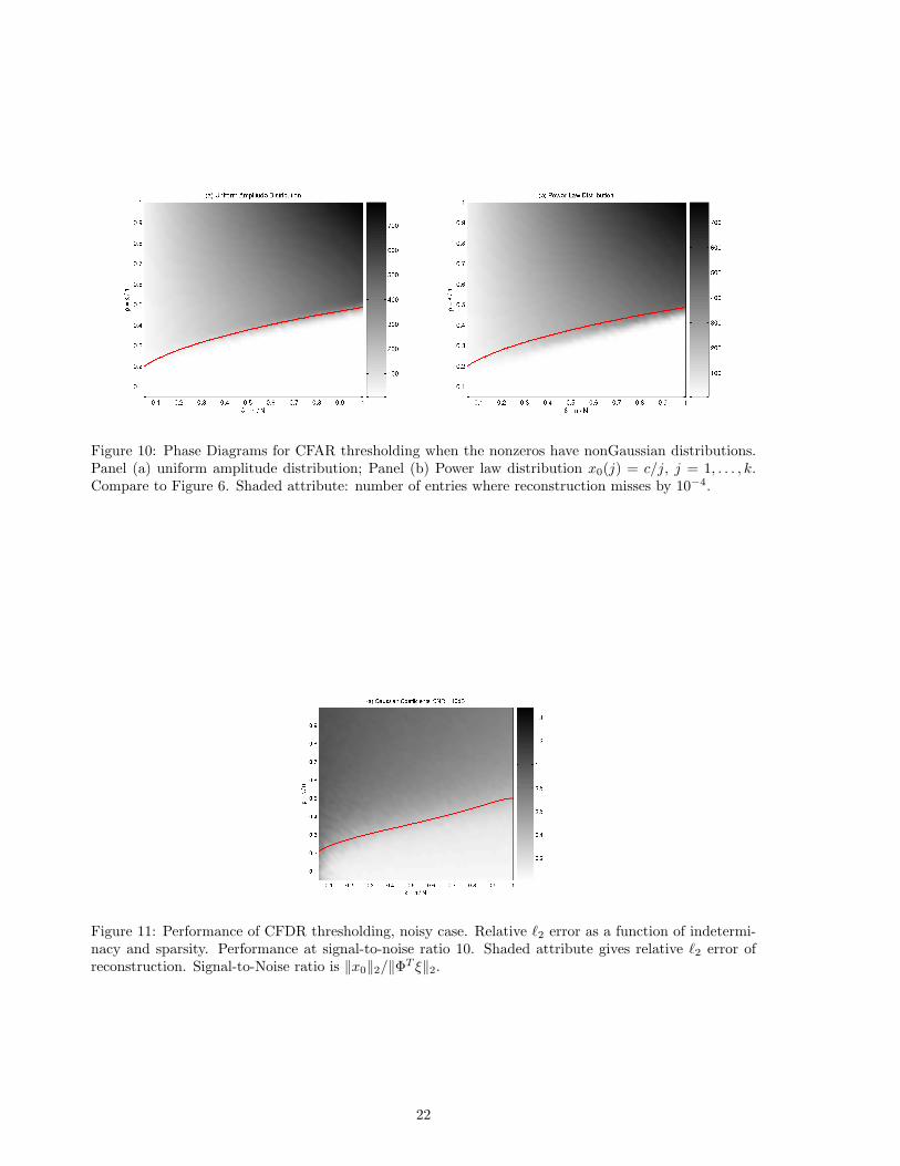
Figure 10: Phase Diagrams for CFAR thresholding when the nonzeros have nonGaussian distributions.Panel (a) uniform amplitude distribution; Panel (b) Power law distribution x0(j) = c/j, j = 1, . . . , k.Compare to Figure 6. Shaded attribute: number of entries where reconstruction misses by 10−4.

Figure 11: Performance of CFDR thresholding, noisy case. Relative `2 error as a function of indetermi-nacy and sparsity. Performance at signal-to-noise ratio 10. Shaded attribute gives relative `2 error ofreconstruction. Signal-to-Noise ratio is ‖x0‖2/‖ΦT ξ‖2.

22

8.4 Other Matrix Ensembles

Our attention has focused on the case where Φ is a random matrix, generated from the uniform sphericalensemble. Similar results follow immediately for two closely related ensembles:

URPE Uniform Random Projection ensemble. Φ contains the first n rows of an N by N randomorthogonal matrix [8]; and

GE Gaussian ensemble. The entries of Φ are iid N(0, 1/n).

In fact we have already used (more than once) the fact that GE and USE are intimately related. Matricesin the two ensembles differ only by the normalization of the columns – a member of URP can beobtained by sampling from the Gaussian ensemble and normalizing the columns to unit length. Also,the close relationship of URPE and GE is quite evident by viewing one as produced from the otherby a Gram-Schmidt process on the rows. Figure 3 Panels(c),(f), and (i) show that for the URPE, theMAI for matched filtering obeys the Gaussian approximation. Extensive experiments have shown thatStOMPhas the same behavior at the URPE, GE, and USE, but we omit details for reasons of space.Scripts generating such experiments are included in the software publication; see Section 10.

More interestingly, we considered other random ensembles, the most well-known ones being

• Random Signs ensemble. The entries of the matrix are ±1/√n, the signs chosen randomly.

• Partial Fourier ensemble. n rows are chosen at random from an N by N Fourier matrix.

• Partial Hadamard ensemble. n rows are chosen at random from an N by N Hadamard matrix.(Possible only for certain N).

These are important for various applications of compressed sensing. For each ensemble, we foundthat the Gaussian approximation applies. Figure 3 Panels(b),(e), and (h) illustrate the MAI for matchedfiltering at the RSE. Thus, we propose StOMP for such ensembles as well.

9 Stylized Applications

We now illustrate the performance of StOMP and the thresholding strategies.

9.1 Compressed Sensing

Recently, there has been considerable interest both from theorists [33, 7, 17, 8] and from practitioners[42, 47, 31, 40, 41] in the possibility of dramatically reducing the ‘number of samples’ that ‘have to bemeasured’ in various remote sensing problems. In effect, one views the problem as one of reconstructinga high-dimensional vector x0 ∈ RN from a low-dimensional data sample y ∈ Rn, which is obtainedfrom x0 by linear sampling. Here although N samples ‘seem to be needed’ according to standard linearalgebra, everything we have shown in this paper (as well as the cited prior work) shows that n < Nsamples can suffice to get either an exact or approximate reconstruction of x0.

We now study the performance of StOMPand the thresholding strategies in concrete instances,inspired by applications in spectroscopy and imaging.

9.1.1 Bumps

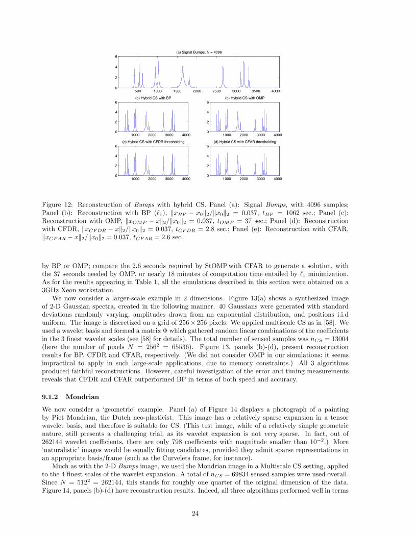
Our first example uses the object Bumps from the Wavelab package [5], rendered with N = 4096 samples.This object, shown in panel (a) of Figure 12, is a caricature of signals arising in NMR spectroscopy, char-acterized by a few localized peaks. Such signals are known to have wavelet expansions with relatively fewsignificant coefficients. We considered a Compressed Sensing (CS) scenario where nCS = 640 sensed sam-ples are taken, reflecting random linear combinations of the wavelet coefficients of Bumps. The details arethe same as for hybrid CS in [58]. In our simulations, we compared the performance of StOMP equippedwith CFDR and CFAR thresholding to that of Basis Pursuit (i.e. `1 minimization) and Matching Pursuit(i.e. OMP). The results are summarized in Figure 12. Evidently, the accuracy of reconstruction is com-parable for all the algorithms used. However, the speed of the two StOMP implementations is unrivaled

23

500 1000 1500 2000 2500 3000 3500 40000

2

4

6(a) Signal Bumps, N = 4096

1000 2000 3000 40000

2

4

6(b) Hybrid CS with BP

1000 2000 3000 40000

2

4

6(b) Hybrid CS with OMP

1000 2000 3000 40000

2

4

6(c) Hybrid CS with CFDR thresholding

1000 2000 3000 40000

2

4

6(d) Hybrid CS with CFAR thresholding

Figure 12: Reconstruction of Bumps with hybrid CS. Panel (a): Signal Bumps, with 4096 samples;Panel (b): Reconstruction with BP (`1), ‖xBP − x0‖2/‖x0‖2 = 0.037, tBP = 1062 sec.; Panel (c):Reconstruction with OMP, ‖xOMP − x‖2/‖x0‖2 = 0.037, tOMP = 37 sec.; Panel (d): Reconstructionwith CFDR, ‖xCFDR − x‖2/‖x0‖2 = 0.037, tCFDR = 2.8 sec.; Panel (e): Reconstruction with CFAR,‖xCFAR − x‖2/‖x0‖2 = 0.037, tCFAR = 2.6 sec.

by BP or OMP; compare the 2.6 seconds required by StOMPwith CFAR to generate a solution, withthe 37 seconds needed by OMP, or nearly 18 minutes of computation time entailed by `1 minimization.As for the results appearing in Table 1, all the simulations described in this section were obtained on a3GHz Xeon workstation.

We now consider a larger-scale example in 2 dimensions. Figure 13(a) shows a synthesized imageof 2-D Gaussian spectra, created in the following manner. 40 Gaussians were generated with standarddeviations randomly varying, amplitudes drawn from an exponential distribution, and positions i.i.duniform. The image is discretized on a grid of 256× 256 pixels. We applied multiscale CS as in [58]. Weused a wavelet basis and formed a matrix Φ which gathered random linear combinations of the coefficientsin the 3 finest wavelet scales (see [58] for details). The total number of sensed samples was nCS = 13004(here the number of pixels N = 2562 = 65536). Figure 13, panels (b)-(d), present reconstructionresults for BP, CFDR and CFAR, respectively. (We did not consider OMP in our simulations; it seemsimpractical to apply in such large-scale applications, due to memory constraints.) All 3 algorithmsproduced faithful reconstructions. However, careful investigation of the error and timing measurementsreveals that CFDR and CFAR outperformed BP in terms of both speed and accuracy.

9.1.2 Mondrian

We now consider a ‘geometric’ example. Panel (a) of Figure 14 displays a photograph of a paintingby Piet Mondrian, the Dutch neo-plasticist. This image has a relatively sparse expansion in a tensorwavelet basis, and therefore is suitable for CS. (This test image, while of a relatively simple geometricnature, still presents a challenging trial, as its wavelet expansion is not very sparse. In fact, out of262144 wavelet coefficients, there are only 798 coefficients with magnitude smaller than 10−2.) More‘naturalistic’ images would be equally fitting candidates, provided they admit sparse representations inan appropriate basis/frame (such as the Curvelets frame, for instance).

Much as with the 2-D Bumps image, we used the Mondrian image in a Multiscale CS setting, appliedto the 4 finest scales of the wavelet expansion. A total of nCS = 69834 sensed samples were used overall.Since N = 5122 = 262144, this stands for roughly one quarter of the original dimension of the data.Figure 14, panels (b)-(d) have reconstruction results. Indeed, all three algorithms performed well in terms

24

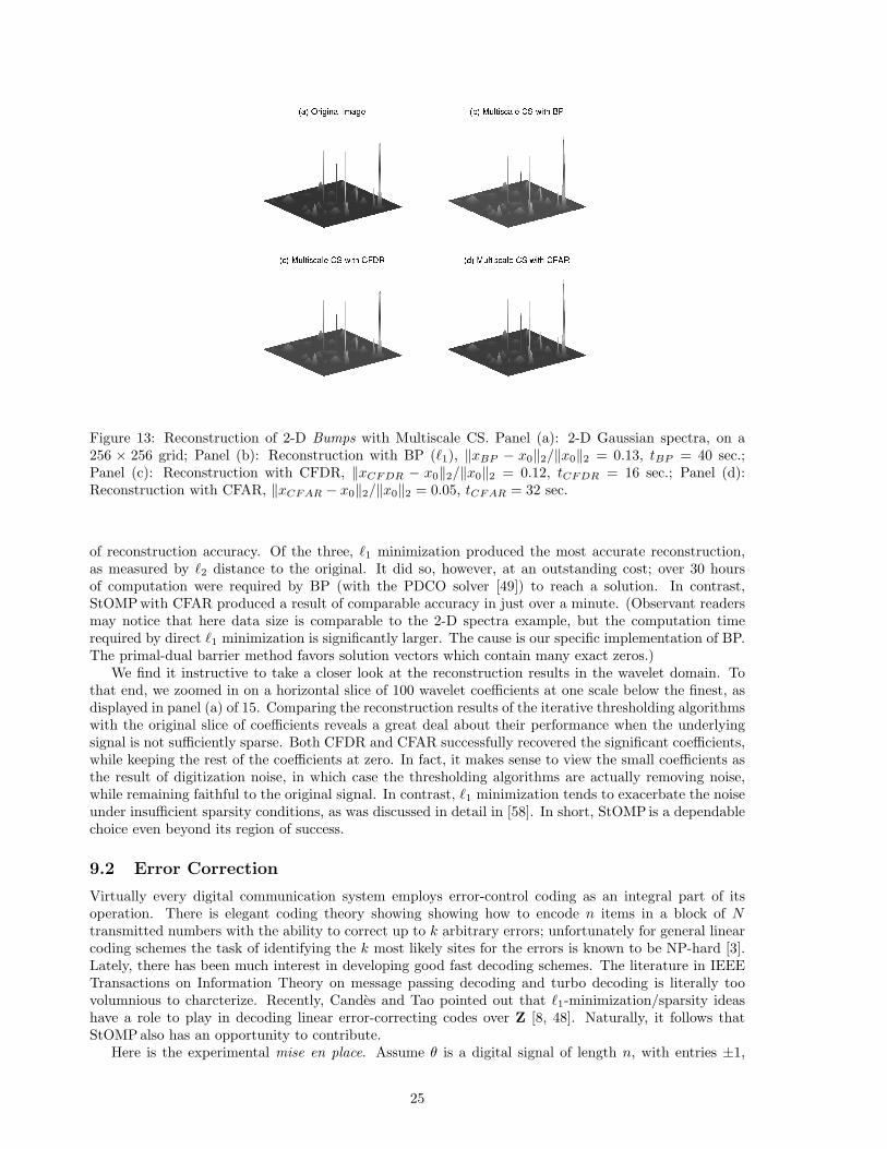
Figure 13: Reconstruction of 2-D Bumps with Multiscale CS. Panel (a): 2-D Gaussian spectra, on a256 × 256 grid; Panel (b): Reconstruction with BP (`1), ‖xBP − x0‖2/‖x0‖2 = 0.13, tBP = 40 sec.;Panel (c): Reconstruction with CFDR, ‖xCFDR − x0‖2/‖x0‖2 = 0.12, tCFDR = 16 sec.; Panel (d):Reconstruction with CFAR, ‖xCFAR − x0‖2/‖x0‖2 = 0.05, tCFAR = 32 sec.

of reconstruction accuracy. Of the three, `1 minimization produced the most accurate reconstruction,as measured by `2 distance to the original. It did so, however, at an outstanding cost; over 30 hoursof computation were required by BP (with the PDCO solver [49]) to reach a solution. In contrast,StOMPwith CFAR produced a result of comparable accuracy in just over a minute. (Observant readersmay notice that here data size is comparable to the 2-D spectra example, but the computation timerequired by direct `1 minimization is significantly larger. The cause is our specific implementation of BP.The primal-dual barrier method favors solution vectors which contain many exact zeros.)

We find it instructive to take a closer look at the reconstruction results in the wavelet domain. Tothat end, we zoomed in on a horizontal slice of 100 wavelet coefficients at one scale below the finest, asdisplayed in panel (a) of 15. Comparing the reconstruction results of the iterative thresholding algorithmswith the original slice of coefficients reveals a great deal about their performance when the underlyingsignal is not sufficiently sparse. Both CFDR and CFAR successfully recovered the significant coefficients,while keeping the rest of the coefficients at zero. In fact, it makes sense to view the small coefficients asthe result of digitization noise, in which case the thresholding algorithms are actually removing noise,while remaining faithful to the original signal. In contrast, `1 minimization tends to exacerbate the noiseunder insufficient sparsity conditions, as was discussed in detail in [58]. In short, StOMP is a dependablechoice even beyond its region of success.

9.2 Error Correction

Virtually every digital communication system employs error-control coding as an integral part of itsoperation. There is elegant coding theory showing showing how to encode n items in a block of Ntransmitted numbers with the ability to correct up to k arbitrary errors; unfortunately for general linearcoding schemes the task of identifying the k most likely sites for the errors is known to be NP-hard [3].Lately, there has been much interest in developing good fast decoding schemes. The literature in IEEETransactions on Information Theory on message passing decoding and turbo decoding is literally toovolumnious to charcterize. Recently, Candes and Tao pointed out that `1-minimization/sparsity ideashave a role to play in decoding linear error-correcting codes over Z [8, 48]. Naturally, it follows thatStOMPalso has an opportunity to contribute.

Here is the experimental mise en place. Assume θ is a digital signal of length n, with entries ±1,

25

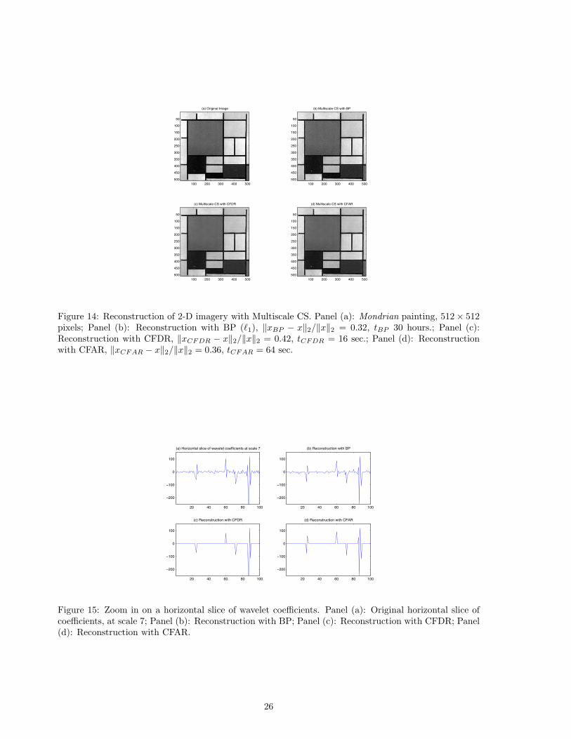
(a) Original Image

100 200 300 400 500

50

100

150

200

250

300

350

400

450

500

(b) Multiscale CS with BP

100 200 300 400 500

50

100

150

200

250

300

350

400

450

500

(c) Multiscale CS with CFDR

100 200 300 400 500

50

100

150

200

250

300

350

400

450

500

(d) Multiscale CS with CFAR

100 200 300 400 500

50

100

150

200

250

300

350

400

450

500

Figure 14: Reconstruction of 2-D imagery with Multiscale CS. Panel (a): Mondrian painting, 512× 512pixels; Panel (b): Reconstruction with BP (`1), ‖xBP − x‖2/‖x‖2 = 0.32, tBP 30 hours.; Panel (c):Reconstruction with CFDR, ‖xCFDR − x‖2/‖x‖2 = 0.42, tCFDR = 16 sec.; Panel (d): Reconstructionwith CFAR, ‖xCFAR − x‖2/‖x‖2 = 0.36, tCFAR = 64 sec.

20 40 60 80 100

−200

−100

0

100

(a) Horizontal slice of wavelet coefficients at scale 7

20 40 60 80 100

−200

−100

0

100

(b) Reconstruction with BP

20 40 60 80 100

−200

−100

0

100

(c) Reconstruction with CFDR

20 40 60 80 100

−200

−100

0

100

(d) Reconstruction with CFAR

Figure 15: Zoom in on a horizontal slice of wavelet coefficients. Panel (a): Original horizontal slice ofcoefficients, at scale 7; Panel (b): Reconstruction with BP; Panel (c): Reconstruction with CFDR; Panel(d): Reconstruction with CFAR.

26

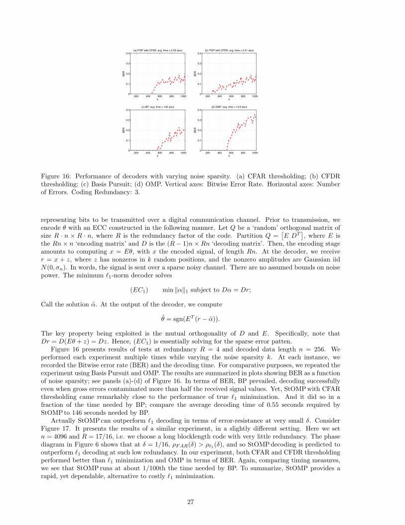
200 400 600 800 10000

0.1

0.2

0.3

0.4

BE

R

k

(a) ITSP with CFAR, avg. time = 0.55 secs

200 400 600 800 10000

0.1

0.2

0.3

0.4

BE

R

k

(b) ITSP with CFDR, avg. time = 0.21 secs

200 400 600 800 10000

0.1

0.2

0.3

0.4

BE

R

k

(c) BP, avg. time = 146 secs

200 400 600 800 10000

0.1

0.2

0.3

0.4

BE

R

k

(d) OMP, avg. time = 13.9 secs

Figure 16: Performance of decoders with varying noise sparsity. (a) CFAR thresholding; (b) CFDRthresholding; (c) Basis Pursuit; (d) OMP. Vertical axes: Bitwise Error Rate. Horizontal axes: Numberof Errors. Coding Redundancy: 3.

representing bits to be transmitted over a digital communication channel. Prior to transmission, weencode θ with an ECC constructed in the following manner. Let Q be a ‘random’ orthogonal matrix ofsize R · n × R · n, where R is the redundancy factor of the code. Partition Q =

[E DT

], where E is

the Rn× n ‘encoding matrix’ and D is the (R− 1)n×Rn ‘decoding matrix’. Then, the encoding stageamounts to computing x = Eθ, with x the encoded signal, of length Rn. At the decoder, we receiver = x + z, where z has nonzeros in k random positions, and the nonzero amplitudes are Gaussian iidN(0, σn). In words, the signal is sent over a sparse noisy channel. There are no assumed bounds on noisepower. The minimum `1-norm decoder solves

(EC1) min ‖α‖1 subject to Dα = Dr;

Call the solution α. At the output of the decoder, we compute

θ = sgn(ET (r − α)).

The key property being exploited is the mutual orthogonality of D and E. Specifically, note thatDr = D(Eθ + z) = Dz. Hence, (EC1) is essentially solving for the sparse error patten.

Figure 16 presents results of tests at redundancy R = 4 and decoded data length n = 256. Weperformed each experiment multiple times while varying the noise sparsity k. At each instance, werecorded the Bitwise error rate (BER) and the decoding time. For comparative purposes, we repeated theexperiment using Basis Pursuit and OMP. The results are summarized in plots showing BER as a functionof noise sparsity; see panels (a)-(d) of Figure 16. In terms of BER, BP prevailed, decoding successfullyeven when gross errors contaminated more than half the received signal values. Yet, StOMP with CFARthresholding came remarkably close to the performance of true `1 minimization. And it did so in afraction of the time needed by BP; compare the average decoding time of 0.55 seconds required byStOMPto 146 seconds needed by BP.

Actually StOMP can outperform `1 decoding in terms of error-resistance at very small δ. ConsiderFigure 17. It presents the results of a similar experiment, in a slightly different setting. Here we setn = 4096 and R = 17/16, i.e. we choose a long blocklength code with very little redundancy. The phasediagram in Figure 6 shows that at δ = 1/16, ρFAR(δ) > ρ`1(δ), and so StOMPdecoding is predicted tooutperform `1 decoding at such low redundancy. In our experiment, both CFAR and CFDR thresholdingperformed better than `1 minimization and OMP in terms of BER. Again, comparing timing measures,we see that StOMPruns at about 1/100th the time needed by BP. To summarize, StOMP provides arapid, yet dependable, alternative to costly `1 minimization.

27

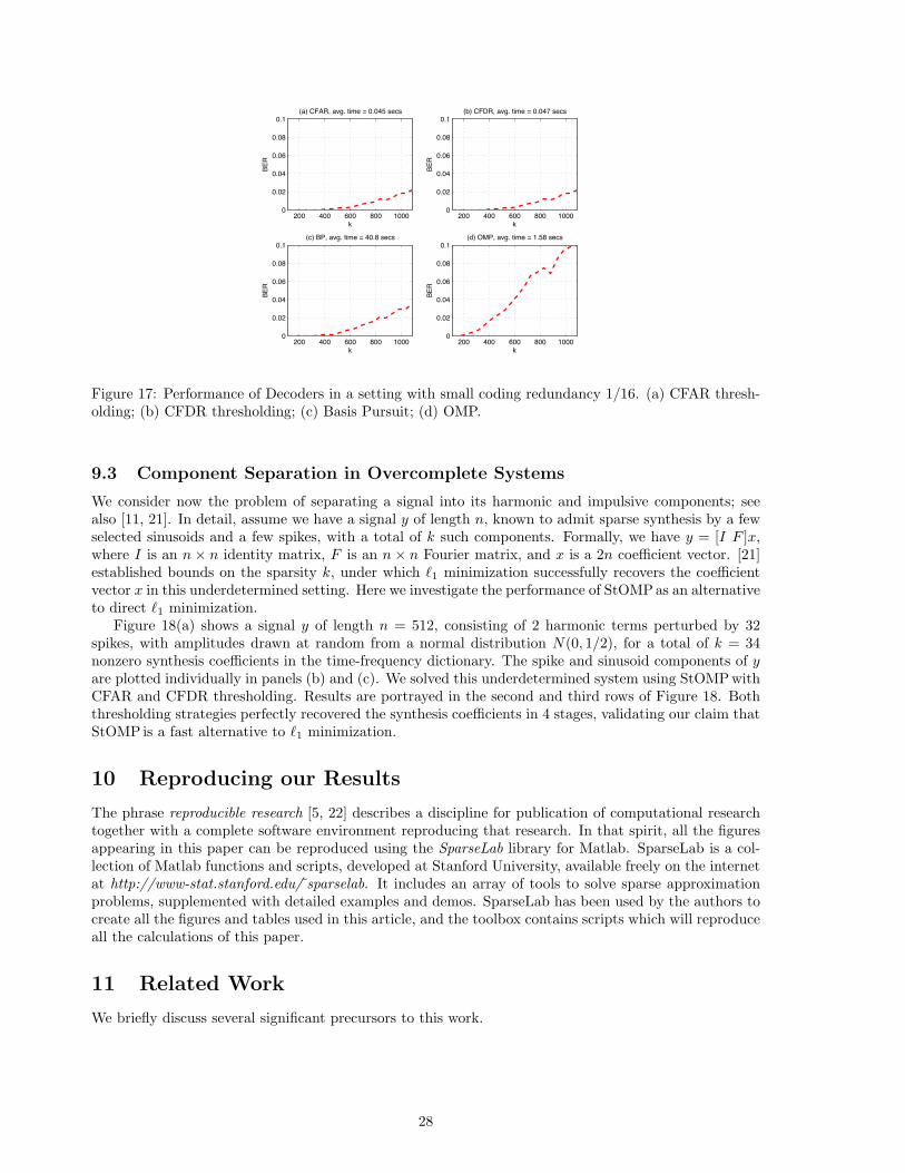
200 400 600 800 10000

0.02

0.04

0.06

0.08

0.1

BE

R

k

(a) CFAR, avg. time = 0.045 secs

200 400 600 800 10000

0.02

0.04

0.06

0.08

0.1

BE

R

k

(b) CFDR, avg. time = 0.047 secs

200 400 600 800 10000

0.02

0.04

0.06

0.08

0.1

BE

R

k

(c) BP, avg. time = 40.8 secs

200 400 600 800 10000

0.02

0.04

0.06

0.08

0.1

BE

R

k

(d) OMP, avg. time = 1.58 secs

Figure 17: Performance of Decoders in a setting with small coding redundancy 1/16. (a) CFAR thresh-olding; (b) CFDR thresholding; (c) Basis Pursuit; (d) OMP.

9.3 Component Separation in Overcomplete Systems

We consider now the problem of separating a signal into its harmonic and impulsive components; seealso [11, 21]. In detail, assume we have a signal y of length n, known to admit sparse synthesis by a fewselected sinusoids and a few spikes, with a total of k such components. Formally, we have y = [I F ]x,where I is an n× n identity matrix, F is an n× n Fourier matrix, and x is a 2n coefficient vector. [21]established bounds on the sparsity k, under which `1 minimization successfully recovers the coefficientvector x in this underdetermined setting. Here we investigate the performance of StOMPas an alternativeto direct `1 minimization.

Figure 18(a) shows a signal y of length n = 512, consisting of 2 harmonic terms perturbed by 32spikes, with amplitudes drawn at random from a normal distribution N(0, 1/2), for a total of k = 34nonzero synthesis coefficients in the time-frequency dictionary. The spike and sinusoid components of yare plotted individually in panels (b) and (c). We solved this underdetermined system using StOMP withCFAR and CFDR thresholding. Results are portrayed in the second and third rows of Figure 18. Boththresholding strategies perfectly recovered the synthesis coefficients in 4 stages, validating our claim thatStOMP is a fast alternative to `1 minimization.

10 Reproducing our Results

The phrase reproducible research [5, 22] describes a discipline for publication of computational researchtogether with a complete software environment reproducing that research. In that spirit, all the figuresappearing in this paper can be reproduced using the SparseLab library for Matlab. SparseLab is a col-lection of Matlab functions and scripts, developed at Stanford University, available freely on the internetat http://www-stat.stanford.edu/ sparselab. It includes an array of tools to solve sparse approximationproblems, supplemented with detailed examples and demos. SparseLab has been used by the authors tocreate all the figures and tables used in this article, and the toolbox contains scripts which will reproduceall the calculations of this paper.

11 Related Work

We briefly discuss several significant precursors to this work.

28

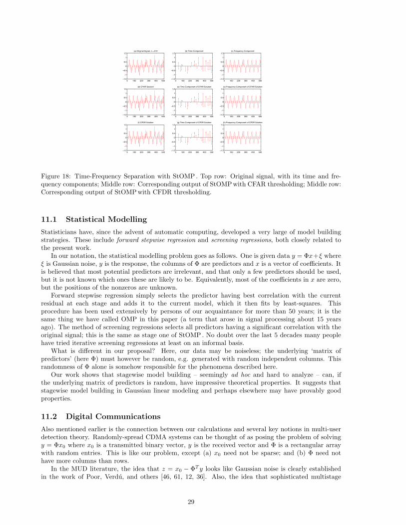
0 100 200 300 400 500−1.5

−1

−0.5

0

0.5

1

1.5(a) Original Signal, n = 512

0 100 200 300 400 500−1.5

−1

−0.5

0

0.5

1

1.5(b) Time Component

0 100 200 300 400 500−1.5

−1

−0.5

0

0.5

1

1.5(c) Frequency Component

0 100 200 300 400 500−1.5

−1

−0.5

0

0.5

1

1.5(d) CFAR Solution

0 100 200 300 400 500−1.5

−1

−0.5

0

0.5

1

1.5(e) Time Component of CFAR Solution

0 100 200 300 400 500−1.5

−1

−0.5

0

0.5

1

1.5(e) Frequency Component of CFAR Solution

0 100 200 300 400 500−1.5

−1

−0.5

0

0.5

1

1.5(f) CFDR Solution

0 100 200 300 400 500−1.5

−1

−0.5

0

0.5

1

1.5(g) Time Component of CFDR Solution

0 100 200 300 400 500−1.5

−1

−0.5

0

0.5

1

1.5(h) Frequency Component of CFDR Solution

Figure 18: Time-Frequency Separation with StOMP . Top row: Original signal, with its time and fre-quency components; Middle row: Corresponding output of StOMP with CFAR thresholding; Middle row:Corresponding output of StOMPwith CFDR thresholding.

11.1 Statistical Modelling

Statisticians have, since the advent of automatic computing, developed a very large of model buildingstrategies. These include forward stepwise regression and screening regressions, both closely related tothe present work.

In our notation, the statistical modelling problem goes as follows. One is given data y = Φx+ξ whereξ is Gaussian noise, y is the response, the columns of Φ are predictors and x is a vector of coefficients. Itis believed that most potential predictors are irrelevant, and that only a few predictors should be used,but it is not known which ones these are likely to be. Equivalently, most of the coefficients in x are zero,but the positions of the nonzeros are unknown.

Forward stepwise regression simply selects the predictor having best correlation with the currentresidual at each stage and adds it to the current model, which it then fits by least-squares. Thisprocedure has been used extensively by persons of our acquaintance for more than 50 years; it is thesame thing we have called OMP in this paper (a term that arose in signal processing about 15 yearsago). The method of screening regressions selects all predictors having a significant correlation with theoriginal signal; this is the same as stage one of StOMP . No doubt over the last 5 decades many peoplehave tried iterative screening regressions at least on an informal basis.

What is different in our proposal? Here, our data may be noiseless; the underlying ‘matrix ofpredictors’ (here Φ) must however be random, e.g. generated with random independent columns. Thisrandomness of Φ alone is somehow responsible for the phenomena described here.

Our work shows that stagewise model building – seemingly ad hoc and hard to analyze – can, ifthe underlying matrix of predictors is random, have impressive theoretical properties. It suggests thatstagewise model building in Gaussian linear modeling and perhaps elsewhere may have provably goodproperties.

11.2 Digital Communications

Also mentioned earlier is the connection between our calculations and several key notions in multi-userdetection theory. Randomly-spread CDMA systems can be thought of as posing the problem of solvingy = Φx0 where x0 is a transmitted binary vector, y is the received vector and Φ is a rectangular arraywith random entries. This is like our problem, except (a) x0 need not be sparse; and (b) Φ need nothave more columns than rows.

In the MUD literature, the idea that z = x0 − ΦT y looks like Gaussian noise is clearly establishedin the work of Poor, Verdu, and others [46, 61, 12, 36]. Also, the idea that sophisticated multistage

29

algorithms can be applied to successively reduce MAI – e.g. onion-peeling schemes [10] or iterativedecoders [4, 6, 13] - is completely consistent with our approach in this paper: stagewise least-squaresprojection when the nonzeros in x0 have a power-law distribution is something like onion-peeling; `1minimization is something like a Bayesian maximum a posteriori iterative decoder. Finally the specificanalysis technique we have developed – the conditioned Gaussian limit – bears some resemblance todensity evolution schemes used in the MUD/CDMA literature, eg [4, 6, 13, 30].

However, there are important differences in the problem, the primary one being that in the binaryCDMA case the vector x0 is not sparse and takes known values ±1, which cause important differencesin results. Also (perhaps) the study of very large N and n is less of interest in CDMA at the moment.

11.3 Component Separation

The immediate inspiration for this paper was extensive work by Jean-Luc Starck and Michael Elad[50, 51] who attacked very large-scale problems in image processing and component separation. Theyfound that by stagewise application of hard thresholding, residualization, and matched filtering, theycould often obtain results comparable to `1 optimization but much more rapidly. Our paper arose fromStarck’s insistence that such an approach was essential to attacking very large scale problems with N inthe millions, and demanded theoretical attention. Focusing on the special case of ‘random’ Φ, we foundhis insistence to be prophetic.

11.4 Mathematical Analysis

The mathematical developments in this paper, and the form of the StOMP algorithm itself, arise froma lemma in the paper [16, Section 5] by one of the authors. That lemma concerned behavior of randomlinear programs, and was originally developed in order to show that `1-minimzation can find sparsesolutions when Φ is drawn from USE; the authors noticed that it implicitly introduces the conditionedGaussian model developed here.

11.5 Fine Points

Two small but essential points:

• The notion of phase transition considered here is weaker than notions often mentioned in connectionwith the study of `1 optimization. As the papers [18, 19] may help clarify, much of the literaturediscusses the notion of strong equivalence of `1 and `0; in this notion that for a given Φ, everysparse x0 generates a problem (y,Φ) for which the `1 solution is the unique sparsest solution[21, 20, 16, 32, 35, 48, 55, 8, 9]. In contrast, in discussing `1 minimization in Section 4.2 above,we used the notion of weak equivalence, which says that equivalence holds for the typical sparse x0

(rather than for every sparse x0) .

In the setting of random matrices Φ sampled from the uniform spherical ensemble, independently ofx0, strong equivalence is not the relevant notion, even though it has attracted the most theoreticalattention. If Φ is random and x0 is fixed in advance, then x0 is overwhelmingly likely to be typicalfor the realized Φ. The empirically observable phase transition is thus the weak transition, whosetheoretical large-system transition point for `1 minimization was derived in [19] and is given by thecurve in Figure 5. For parallel discussion see [54].

The notion discussed here for StOMP is still weaker, because our probabilistic theory only stud-ies approximate reconstruction of typical x0. Hence it might seem that the phase transition forStOMPmapped out here is less useful in practice than the weak equivalence transition for `1 min-imization. Despite this, empirically we have found that for N = 1600, below its phase transitioncurve StOMPyields reconstructions which are numerically just as accurate as `1 minimization yieldsbelow its phase transition curve.

• Iterative thresholding is an algorithm which, like StOMP , successively strips structure out of aresidual vector; like StOMP , it computes the vector of current correlations cs = ΦT rs and appliesa threshold; however, instead of orthogonal projection to remove detected structure, it uses a

30

relaxation strategy rs+1 = rs − λ · A · Threshold(cs), subtracting structure associated to columnssurviving thresholding.

The use of alternating thresholding to obtain sparse solution has been extensively deployed byStarck and co-workers [50, 51] and studied by Daubechies and co-workers [15]. An early referenceapplying a kind of alternating thresholding to seek sparse solutions to underdetermined systems wasCoifman and Wickerhauser (1993) [14]. To our knowledge, the alternating thresholding approachhas yielded today’s most successful applications of large-scale sparse solutions [40, 41, 50, 51].

StOMP is subtly, but crucially different; our inspiration is the idea that for Gaussian randommatrices Φ (and their close relatives), selection followed by projection affords certain definite prob-abilistic structure, which we have exposed and analyzed carefully here, in Theorems 1,2, and 3.The initially similar-sounding proposals for alternating soft and hard thresholding do not seem tooffer any comparably strong analytic framework.

12 Summary

We described a simple algorithm for obtaining sparse approximate solutions of certain underdeterminedsystems of linear equations. The StOMPalgorithm iteratively thresholds, selects and projects. It selectsnonzeros by thresholding the output of the matched filter applied to the current residual signal, wherethe threshold is set above the mutual interference level. It projects the residual on a lower-dimensionalsubspace complementary to the span of the selected nonzeros.

StOMP is effective when the matrix Φ and/or the object x0 render the multiple access interferenceapproximately Gaussian. Relying on such Gaussianity, we proposed two natural strategies for thresholdselection, one based on false alarm rate control and one based on false discovery rate control.

We rated the success of this approach using the phase diagram and showed that, in the standardproblem suite, for either thresholding rule the phase diagram has two phases – success and failure –with a narrow transition zone between them. The transition zone shrinks in size as the problem sizegrows. For each method, the “success phase” of StOMP is comparable in size to the “success phase”of `1 minimization. Computational experiments showed that within the intersection of the two successphases, StOMP can deliver results comparable to l1 minimization with dramatically less computation.Also, in numerous examples StOMP runs much faster than standard greedy approximation (matchingpursuit).

Supporting the practical advantages of StOMP is a theoretical framework that accurately derives theboundary of the success phase. This boundary can be regarded as a well-defined asymptotic “samplingtheory” for StOMP ; to reconstruct a sparse vector by StOMP , an asymptotically precise number ofsamples will be required.

StOMPextends naturally to noisy data, and also extends to underdetermined systems outside the‘random’ ones where the method was derived, important examples being the partial Fourier ensemble andpairs of incoherent orthogonal bases such as (Dirac,Fourier). Stylized applications in compressed sensing,suppression of impulsive noise, and time-frequency separation are given, and software is available.

Appendices

A: Proof of Lemma 1

Consider the restriction xS = xS |IS, i.e. ‘throw away’ the entries in xS lying outside IS . By hypothesis

all the entries that are thrown out are zero, and the residual from StOMP is zero, so y = ΦISxS .

Similarly, consider the restriction x0 = x0|IS, i.e. form the vector x0 with entries outside of IS thrown

away. Since by hypothesis, x0 is supported inside IS , we also have y = ΦISx0.

Hence 0 = ΦIS(xS − x0). By hypothesis the columns of Φ are in general position, so there is no

nontrivial relation 0 = ΦISv where #IS < n and v is a column vector compatible with ΦIS

. HencexS = x0 and also xS = x0. �

31

B: Heuristic Phase Transition Calculation for the Standard Ensemble

We have found that the following heuristic model can be used to derive a predicted phase transitioncurve that qualitatively matches the behavior of the empirical phase transition in the standard problemsuite. We use notation paralleling the notation of Section 6.

Under this heuristic, the normalized coefficients 〈φi, rs〉/‖Qsφi‖2 for i ∈ Ics−1 act as random samples

from a Gaussian mixture distribution:

(1− εs)N(0, σ2s) + εsN(0, 1).

where εs = ks/Ns and σs =√ks/ns.

We therefore defineαs = P{|N(0, σ2

s)| > ts · σs},

andβs = P{|N(0, 1)| > ts · σs}.

We start with (ρ1, d1, ν1, σ1) = (ρ, 1, 1/δ, ρ) and apply the obvious updating formulas

ds+1 = ds − αs(νs − ρs)− βsρs

ρs+1 = ρs − (1− βs)ρs

νs+1 = νs − (1− αs)(νs − ρs) + (ρs+1 − ρs)

σs+1 =

√ρs+1

ds+1

.

If, at or before stage S, we achieve ds > η and ρs < η · ρ, we declare StOMPto be successful at thatgiven (δ, ρ).

For CFAR thresholding, ts is constant, set to the 1−αS/2 quantile of the standard normal distribution,where αS = 1− ( 1−δ

1−ρδ )1/S . For CFDR thresholding, ts is variable, set to the solution of

P{|N(0, σ2s)| > tσs}

P{|N(0, 1)| > tσs}=

εs1− εs

· q

1− q.

Here q is the assumed false discovery rate; we used 1/2 in all our work.These heuristic formulas cannot be precisely correct, for two reasons: (i) they omit the effect of

conditioning caused by earlier stages, as discussed in Section 7 – the underlying coefficient distributionis a mixture, but not of normal distributions; and (ii) the pseudo-standard deviation is merely a crudeupper bound; the true value reflects considerations from random matrix theory.

However, if the variance σs drops very rapidly with increasing s, often this heuristic is reasonablyaccurate.

C: Proof of Theorem 1

By state vector hs,n we mean a four-tuple

hs,n = (ks,n

n,ns,n

n,Ns,n

n,‖rs‖2

2

n), 1 ≤ s ≤ S + 1;

note that this is a random variable. For s = 1 we have

h1,n = (kn

n, 1,

Nn

n,‖y‖2

2

n);

while later steps depend on the specific realization (y,Φ) and the progress of the algorithm. Note that ifat step ` < S, n`,n = 0, so the algorithm must stop prior to planned termination, we put, by definition

hs,n = h`,n, ` ≤ s ≤ S + 1.

The distance between two state vectors d(h, h′) is just the Euclidean distance between the 4-tuples.

32

By history Hs,n we mean the sequence of state vectors up to stage s,

Hs,n = (h1,n, . . . , hs,n).

This is again a random variable. By distance between two histories we mean the maximal distancebetween corresponding states of the history:

d(Hs,H′s) = max

1≤`≤sd(h`, h

′`).

We now observe that all the quantities αs,n, . . . , νs,n defined in the statement of Theorem 1 areuniformly continuous functions of the history Hs+1,n. Therefore, it is sufficient to prove that there existsa large-system limit for the history HS+1,n, i.e. that, given (δ, ρ), there is HS+1(δ, ρ) so that for eachε > 0,

Pn{d(HS+1,n, HS+1) > ε} → 0, n→∞. (12.1)

This can be done inductively, as follows. First, for s = 1, recall that we assume y =∑k

`=1±`φi`. We

have, by elementary calculations,

p.limn→∞

‖y‖22/n = lim

n→∞kn/n = ρ.

This proves:

Lemma 12.1 (Large-system limit, s = 1) Let n/Nn → δ and kn/n→ ρ as n→∞. Then

p.limn→∞

h1,n = h1(δ, ρ) ≡ (ρ, 1, δ−1, ρ). (12.2)

Hence, the inductive process is begun. Below we will show that there is a deterministic sequence (hs :s = 2, . . . , S + 1) obeying

hs+1 = hs −∆s(Hs), s = 1, . . . , S, (12.3)

for certain 4-tuple-valued functions ∆s of s-step histories; for each ε > 0, this sequence obeys

Pn{d(hs+1,n, hs+1) > 2ε|d(hs,n, hs) < ε} → 0, n→∞, s = 1, . . . , S, (12.4)

then (12.1) follows.To establish (12.4) we consider in turn each individual component hs(`), ` = 1, . . . 4. The first three

components share much in common, owing to the similar relations

ks+1 = ks − |Js ∩ I0|, (12.5)

ns+1 = ns − |Js|,

andNs+1 = Ns − |Js|.

Consider the first component hs,n(1) = ks,n/n. In the next subsection we prove the following:

Lemma 12.2 Suppose either that s = 1 or that s > 1 and (12.4) has been proven for 1 ≤ ` ≤ s− 1. LetXs denote the conditioned Gaussian random variable defined as in Section 7 by the sequences (µ` : 1 ≤` ≤ s) and (σ` : 1 ≤ ` ≤ s), where

µs = hs(4)/hs(1), σs =√hs(4). (12.6)

Thenks+1,n

n=ks,n

n(1− P{|Xs| > tσs}) + op(1), n→∞. (12.7)

33

Now of course P{|Xs| > tσs} depends on the limit history Hs; so it makes sense to write ∆s,1(Hs) ≡hs(1) · P{|Xs| > tσs}. Exploiting the result ks,n/n →P hs(1) which we regard as proved at a previousstage of the argument, we rewrite (12.7) as

hs+1(1) = hs(1)−∆s,1(Hs), s = 1, . . . , S.

We can argue very similarly for the second and third components of the state vector, ns/n and Ns/n.Put εs = hs(1)/hs(3), νs = hs(3), and define

∆s,2(Hs) = νs ·[(1− εs) · P{|Zs| > tσs}+ εs · P{|Xs| > tσs}

],

where Xs is a conditioned Gaussian random variable defined by (µs) and (σs) as in (12.6), and whereZs is a conditioned Gaussian random variable with the same σ-sequence but with means µ = 0. Thisdefines a continuous function of s-step histories, and putting ∆s,2 = ∆s,3 one can show

hs+1(`) = hs(`)−∆s,`(Hs), s = 1, . . . , S, ` = 2, 3.

However, the arguments being so similar to those behind Lemma 12.2, we omit them.This leaves only the need to argue for the fourth and final component of the state vector. Now the

analog of (12.5) is‖rs+1‖2

2 = ‖rs‖22 − cTs (ΦT

JsΦJs)

−1cs,

wherecs = ΦT

Jsrs,

and ΦJs is the submatrix of Φ with columns from Js = {j : |cs| > tσs}. The subsection after next proves

Lemma 12.3 Suppose either that s = 1 or that s > 1 and that (12.4) has been proven for 1 ≤ ` ≤s− 1. Let Xs denote the conditioned Gaussian random variable defined as in Section 7 by the sequences(µ` : 1 ≤ ` ≤ s) and (σ` : 1 ≤ ` ≤ s), obeying (12.6). Similarly, let Zs be a conditioned Gaussianrandom variable defined as in Section 7 by µ` = 0 and by (σ` : 1 ≤ ` ≤ s) again as in (12.6). Putεs ≡ hs(1)/hs(3), and define the mixture density

ps(x) = (1− εs) · pZs(x) + εs · pXs

(x).

Put νs ≡ hs(3) and

Γs(Hs) = νs ·∫x21{|x|>tσs}ps(x)dx;

and, with ds ≡ hs(2), set

∆s,4(Hs) ≡Γs(Hs)

ds+1 + Γs(Hs)/σ2s

.

Thenn−1‖rs+1‖2

2 = n−1‖rs‖22 −∆s,4(Hs) + op(1), n→∞.

It follows thaths+1(4) = hs(4)−∆s,4(Hs), s = 1, . . . , S.

This completes the proof of (12.3)-(12.4). �

The Role of Interleaving in Theorems 1,2,3.

We have stated Theorems 1, 2, and 3 in the body of our paper as if they are independent propositions,proved separately. Actually we only present arguments to prove them in an interleaved, sequential fashion.

We think of the 3 theorems as 3S + 1 ‘little’ theorems, call them little Theorem 1`, ` = 1, . . . , S + 1,and little Theorems 2`, 3`, ` = 1, . . . , S. Thus little Theorem 11 yields the special case s = 1 of ‘big’Theorem 1. Little Theorem 12 yields the special case s = 2, etc. This decomposition of the original ‘big’theorems into component theorems involves slightly different hypotheses than the original ones; in fact

34

our proof of little Theorem 1s depends on exploiting the conclusions previously established in provinglittle Theorems 1s−1, 2s−1, and 3s−1.

Thus, our proofs really show that, once little Theorem 11 is proved, little Theorems 21 and 31 can beproved.

Then, little Theorem 12 can be proved, followed by little Theorems 22 and 32.In general, for s > 1, our proof of little Theorem 1s requires that all the little Theorems 1`, for

1 ≤ ` < s be proved as well as the little Theorems 2` and 3`, for 1 ≤ ` < s. We felt it best from anexpository viewpoint to hide this interleaving until now. The interleaving has finally become explicit inthe statement of Lemmas 12.2-12.3 above.

Analysis of ks/n

|Js ∩ I0| =∑

i∈Ics−1∩I0

1{|〈φi,rs〉|>tσs}

=ks∑

`=1

V`,s,

say.Now the (φj : j ∈ I0) are independent identically distributed random vectors. Membership in Ic

s−1 isa condition imposed symmetrically on all of the random vectors in (φj : j ∈ Ic

s−1 ∩ I0). It follows that,conditional on Is−1, these are conditionally exchangeable random variables, which proves:

Lemma 12.4 Conditional on Hs,n, the (V`,s : ` = 1, . . . , ks) are exchangeable random variables.

Exchangeability allows easy characterisation of the mean and variance of n−1∑

` V`. Now

E(V`,s|Hs) = Pn{|〈φi, rs〉| > tσs|i ∈ I0 ∩ Ics−1, I0, Is−1}.

soE(n−1

∑`

V`,s|Hs) =ks

n· Pn{|〈φi, rs〉| > tσs|i ∈ I0 ∩ Ic

s−1, I0, Is−1 };

meanwhile,

V ar(n−1

ks,n∑`=1

V`,s|Hs) = ks/n2 · V ar(V1,s|Hs) + (k2

s − ks)/n2Cov(V1,s, V2,s|Hs).

We now use interleaving. We assume that little Theorems 1`,2`, 3` have all been proved, for 1 ≤ ` ≤ sand we are trying to prove little Theorem 1s+1. Combining Theorems 1s and 3s we obtain

Lemma 12.5 With Xs as in the statement of Lemma 12.2,

limn→∞

Pn{|〈φi, rs〉| > tsσs|i ∈ I0 ∩ Ics−1, I0, Is−1} = P{|Xs| > tσs}.

We omit the proof of the following technical lemma.

Lemma 12.60 = p.lim

n→∞Cov(V1,s, V2,s|Hs,n).

Combining these lemmas proves Lemma 12.2 �

35

Analysis of ‖rs‖22/n

It is enough to show that for ds ≡ hs(2),

p.limn→∞

n−1cTs (ΦTJs

ΦJs)−1cs =

Γs(Hs)ds+1 + Γs(Hs)/σ2

s

. (12.8)

We may choose coordinates in Rns so that rs is aligned with e1, the standard unit vector. Then in factcTs ≡ cTs /‖rs‖2 is the first row of ΦJs and so, letting BJs denote the ns − 1× |Js| matrix consisting of allbut the first row of ΦJs ,

‖rs+1‖22 − ‖rs‖2

2 = cTs (cscTs +BTJsBJs

)−1cs.

The matrix Φ almost has Gaussian iid entries in the following sense. Let D be an ns-by-ns diagonalmatrix with diagonal entries independently and identically distributed as n−1/2

s ×χns , where χd denotesthe usual χ-distribution on d degrees of freedom; in addition let D be stochastically independent of Φ.Then ΦD is a random matrix with Gaussian iid N(0, 1/n) entries.

Hence, conditionally on Is−1, the entries in the matrix Ψ = BJsDJs

are iid Gaussian random variables.Although we omit details, clearly our problem approximately reduces to studying

cTs (cscTs + ΨT Ψ)−1cs.

Invoke now the Sherman-Morrison formula: for a column vector w and a compatible nonsingular matrixA,

wT (wwT +A)−1w =wTA−1w

1 + wTA−1w.

Note now that Ψ is stochastically independent of cs. Pick an orthogonal matrix V ∈ SO(ks) whosefirst column is proportional to cs and which is randomly sampled from the canonical uniform measureon SO(ks) subject to this constraint. Also let V be stochastically independent of Ψ. Define Ψ = ΨV .Now e1 ∝ V cs and by a simple computation,

cTs (ΨT Ψ)−1cs = ‖cs‖2(ΨT Ψ)−111 .

At the same time, Ψ has iid Gaussian N(0, 1/n) entries.Some well-known facts about random Gaussian matrices allow us to study the random diagonal entry

(ΨT Ψ)−11,1; compare the following restatement of results of Bai and Yin quoted in [60]. We omit the proof.

Lemma 12.7 Let Wn be a pn × qn matrix with entries i.i.d. N(0, 1/n). Let (pn − qn)/n → γ > 0 asn→∞. Then

p.limn→∞

(WTn Wn)−1

1,1 =1γ.

In the case of interest to us, pn = |Ics−1| while qn = |Js|. Hence, pn − qn = |Ic

s | and γ = ds+1.We now again use interleaving. We assume that little Theorems 1`,2`, 3` have all been proved, for

1 ≤ ` ≤ s and we are trying to prove the part of little Theorem 1s+1 referring to the fourth componentof hs+1. Restating little Theorems 2s and 3s we obtain that the typical component of cs at indicesi ∈ I0 ∩ Ic

s−1 has approximately the probability distribution of Xs, while the typical component of cs atindices i ∈ Ic

0 ∩ Ics−1 has approximately the probability distribution of Zs. Hence

‖cs,n‖22 =

∑i

〈φi, rs〉21{|〈φi,rs〉|>tσs}

=∑

i∈Ic0∩Ic

s−1

+∑

i∈I0∩Ics−1

∼ (Ns − ks)∫z21{|z|>tσs}pZs

(z)dz + ks

∫x21{|x|>tσs}pXs

(x)dx

∼ n · νs ·∫x21{|x|>tσs}ps(x)dx ∼ n · Γs(Hs).

Lemma 12.8 With Xs as in the statement of Lemma 12.2, We have

p.limn→∞

‖cs,n‖22/n = Γs(Hs).

Combining the above yields (12.8). �

36

References

[1] F. Abramovich, Y. Benjamini, D.L. Donoho and I.M. Johnstone (2006) Adapting to unknown spar-sity by controlling the False Discovery Rate. in press, Annals of Statitsics.

[2] Y. Benjamini and Y. Hochberg (1995) Controlling the false discovery rate: a practical and powerfulapproach to multiple testing. Journal of the Royal Statistical Society, Series B. 57, pp. 289–300.

[3] E.R.Berlekamp, R.J.McEliece, and H.C.A. van Tilborg. (1978) On the inherent intractability ofcertain coding problems. IEEE Trans. Info. Thry., 24:384–386, 1978.

[4] J. Boutros and G. Caire (2002) Iterative multiuser joint decoding: unified framework and asymptoticanalysis. IEEE Trans. Info. Thry. 48 1772-

[5] J. Buckheit and D. L. Donoho (1995) WaveLab and reproducible research, in A. Antoniadis, Editor,Wavelets and Statistics, Springer.

[6] G. Caire, R. Muller and T. Tanaka (2004) Iterative multiuser joint decoding: optimal power alloca-tion and low-complexity implementation. IEEE Trans. Info. Thry. 50(9), pp. 1950–1973.

[7] E.J. Candes, J. Romberg and T. Tao. (2004) Robust Uncertainty Principles: Exact Signal Recon-struction from Highly Incomplete Frequency Information. To Appear, IEEE Trans. Info. Thry.

[8] E.J. Candes and T. Tao. (2004) Near Optimal Signal Recovery From Random Projections: UniversalEncoding Strategies? To Appear, IEEE Trans. Info. Thry.

[9] E.J. Candes and T. Tao. (2005) Decoding via Linear Programming. IEEE Trans. Info. Thry.

[10] Naftali Chayat and Shlomo Shamai (1999) Convergence properties of iterative soft onion peeling. inProc. 1999 IEEE Info. Thry. Workshop, Kruger National Park, South Africa.

[11] S. Chen, D. Donoho, and M.A. Saunders (1999) Atomic Decomposition by Basis Pursuit. SIAM J.Sci Comp., 20(1), pp. 33–61.

[12] E. Chong, J. Zhang, and D. Tse (2001) Output MAI distribution of linear MMSE multiuser receiversin DS-CDMA systems. IEEE Trans. Info. Thry. 47(3), pp. 1128–1144.

[13] S.Y. Chung, T.J. Richardson and R.L. Urbanke (2001) Analysis of Sum-Product decoding of low-density parity-check codes using a Gaussian approximation. IEEE Trans. Info Thry. 47(2), pp.657–670.

[14] Ronald R. Coifman and Mladen Victor Wickerhauser (1993) Wavelets and adapted waveform anal-ysis: A toolkit for signal processing and numerical analysis. In Different Perspectives on Wavelets,Ingrid Daubechies, editor. number 47 in Proceedings of Symposia in Applied Mathematics, AmericanMathematical Society. Providence, Rhode Island.

[15] I. Daubechies, M. Defrise and C. De Mol (2004) An iterative thresholding algorithm for linear inverseproblems with a sparsity constraint Comm. Pure Applied Mathematics 57, 1413 - 1457.

[16] D.L. Donoho (2004) For most large underdetermined systems of linear equations, the minimal `1-norm solution is also the sparsest solution. Submitted. Com.. Pure Appl. Math., to appear 2006.

[17] D.L. Donoho (2004) Compressed sensing. IEEE Trans. Info. Thry., to appear 2006.

[18] D.L. Donoho (2005) Neighborly Polytopes and the Sparse Solution of Underdetermined Systems ofLinear Equations. To appear, IEEE Trans. Info. Thry..

[19] D.L. Donoho (2005) High-dimensional centrosymmetric polytopes with neighborliness proportionalto dimension. to appear, Discrete and Computational Geometry, 2006.

[20] D.L. Donoho and M. Elad (2003) Optimally Sparse Representation from Overcomplete Dictionariesvia `1 norm minimization. Proc. Natl. Acad. Sci. USA, 100(5), pp. 2197–2002.

37

[21] D.L. Donoho and X. Huo (2001) Uncertainty Principles and Ideal Atomic Decomposition. IEEETrans. Info. Thry. 47(7), pp. 2845-62.

[22] D.L. Donoho and X. Huo (2004) BeamLab and Reproducible Research. International Journal ofWavelets, Multiresolution and Information Processing, 2(4), pp. 391–414.

[23] D.L. Donoho and J. Jin (2006) Asymptotic Minimaxity of False Discovery Rate Thresholding forExponential Data. Ann. Statist., to appear.

[24] D.L. Donoho and I.M. Johnstone (1994) Minimax risk over `p-balls for `q-error. Probability Theoryand Related Fields 99, pp. 277–303.

[25] D.L. Donoho and I.M. Johnstone (1994) Ideal spatial adaptation via wavelet shrinkage. Biometrika,81, pp. 425–455.

[26] D.L. Donoho, I.M. Johnstone, A.S. Stern and J.C. Hoch (1992) Maximum Entropy and the NearlyBlack Object (with discussion). Journal of the Royal Statistical Society, Series B, 54(1), pp. 41–81.

[27] D.L. Donoho and I.M. Johnstone (1995) Adapting to unknown smoothness via wavelet shrinkage.J. Amer. Statist. Assoc., 90, pp. 1200–1224.

[28] D.L. Donoho and B.F. Logan (1992) Signal Recovery and the Large Sieve. SIAM Journal of AppliedMath, 52, pp. 577–591.

[29] M. F. Duarte, M.B. Wakin and R.G. Baraniuk (2005) Fast Reconstruction of Piecewise SmoothSignals from Random Projections (Online Proc. SPARS Workshop, Nov. 2005)

[30] H. El Gamal and A.R. Hammons, Jr. (2001) Analyzing the Turbo decoder using the GaussianApproximation. IEEE Trans. Info. Thry., 47(2), pp. 671–686.

[31] Ray Freeman and Eriks Kupce (2003) New Methods for Fast Multidimensional NMR. Journal ofBiomolecular NMR, 27, pp. 101–113.

[32] Jean-Jacques Fuchs (2002) On Sparse Representations in Arbitrary Redundant Bases. IEEE Trans.Info. Thry, 50(6), pp. 1341–44.

[33] A.C. Gilbert, S. Guha, P. Indyk, S. Muthukrishnan and M. Strauss (2002) Near-optimal sparseFourier representations via sampling. Proc 34th ACM symposium on Theory of Computing, pp.152–161, ACM Press.

[34] G. Golub and C. van Loan (1996) Matrix computations, third edition, The Johns Hopkins UniversityPress, London.

[35] R. Gribonval and M. Nielsen (2003) Sparse Representations in Unions of Bases. IEEE Trans. Info.Thry 49(12), pp. 1320–25.

[36] D. Guo, S. Verdu and L. Rasmussen (2002) Asymptotic normality of linear multiuser receiver out-puts. IEEE Trans. Info. Thry. 48(12), 3080-3095.

[37] I.M. Johnstone and B.W. Silverman (2004) Needles and straw in haystacks: empirical Bayes esti-mates of possibly sparse sequences. Annals of Statistics, 32, pp. 1594–1649.

[38] Y. Hochberg and A. Tamhane (1987) Multiple Comparison Procedures, John Wiley & Sons, NewYork.

[39] E. Lehmann and J. Romano (2003) Testing Statistical Hypotheses (3rd edition), Springer, New York.

[40] M. Lustig, J.H. Lee, D.L. Donoho and J.M. Pauly (2004) Faster Imaging with Randomly PerturbedSpirals and L1 Reconstruction. Proc. of the ISMRM 13th annual meeting.

[41] M. Lustig, J.M Santos, D.L. Donoho and J.M. Pauly (2006) Rapid MR Angiography with RandomlyUnder-Sampled 3DFT Trajectories and Non-Linear Reconstruction. Proc. of the SCMR 9th annualScientific meeting, to appear.

38

[42] M.W. Maciejewski, A.S. Stern, G.F. King and J.C. Hoch (2006) Nonuniform Sampling in Biomolec-ular NMR. Handbook of Modern Magnetic Resonance, Graham A. Webb, Springer.

[43] S. Mallat and Z. Zhang (1993) Matching Pursuit with time-frequency dictionaries, IEEE Transac-tions on Signal Processing, 41(12), pp. 3397–3415.

[44] P. McCullagh (1987) Tensor Methods in Statistics, Chapman and Hall.

[45] A. Paulraj, R. Nabar and D. Gore (2003) Introduction to Space-Time Wireless Communications,Cambridge University Press.

[46] H.V. Poor and S. Verdu (1997) Probability of error in MMSE multiuser detection. IEEE Trans.Info. Thry. 43(3), pp. 858–871.

[47] D. Rovnyak, D.P. Frueh, M. Sastry, Z.J. Sun, A.S. Stern, J.C. Hoch and G. Wagner (2004) Ac-celerated acquisition of high resolution triple-resonance spectra using non-uniform sampling andmaximum entropy reconstruction. Journal of Magnetic Resonance, 170(1), pp. 15–21.

[48] M. Rudelson and R. Vershynin (2005) Geometric approach to error-correcting codes and reconstruc-tion of signals. Technical report, Dept. of Mathematics, Univ. of California at Davis.

[49] M. A. Saunders (2002) PDCO: Primal-Dual interior method for Convex Objectives. Available at:http://www.stanford.edu/group/SOL/software/pdco.html

[50] J.-L. Starck, M. Elad and D.L. Donoho (2004) Redundant Multiscale Transforms and their Appli-cation for Morphological Component Analysis. Advances in Imaging and Electron Physics, 132.

[51] J.-L. Starck, M. Elad and D.L. Donoho (2005) Image Decomposition Via the Combination of SparseRepresentation and a Variational Approach. IEEE Trans. Image Proc., 14(10), pp. 1570–1582.

[52] V.N. Temlyakov (1999) Greedy algorithms and m-term approximation, J. Approx. Theory, 98, pp.117–145.

[53] V.N. Temlyakov (2003) Nonlinear methods of approximation. Found. Comput. Math., 3, pp. 33–107.

[54] J.A. Tropp and A. Gilbert (2005) Signal Recovery from Partial Information by Orthogonal MatchingPursuit. Manuscript.

[55] J.A. Tropp (2003) Greed is Good: Algorithmic Results for Sparse Approximation. IEEE Trans Info.Thry. 50(11), pp. 2231–42.

[56] J.A. Tropp (2004) Just Relax: Convex programming methods for Subset Selection and SparseApproximation. Manuscript.

[57] Y. Tsaig and D.L. Donoho (2005) Breakdown of equivalence between the minimal `1-norm solutionand the sparsest solution. EURASIP Journal of Applied Signal Processing, in press.

[58] Y. Tsaig and D.L. Donoho (2005) Extensions of compressed sensing. EURASIP Journal of AppliedSignal Processing, in press.

[59] D.N.C. Tse and S. Verdu (2000) Optimum asymptotic multiuser efficiency of randomly spreadCDMA, IEEE Trans Info. Thry., 46(7), pp. 2718–2722.

[60] S. Verdu. (1998) Multiuser Detection. Cambridge University Press.

[61] S. Verdu and S. Shamai (1999) Spectral efficiency of CDMA with random spreading. IEEE Trans.Info. Thry. 45(2), pp. 622–640.

39