Solution Chapter7
29
Chapter 7 FIR Filter Design 1. Problem P 7.2 Amplitude response function for Type-II LP FIR filter (a) Type-II symmetric hn andM–even, i.e., hn hM 1 n 0 n M 1; α M 1 2 is not an integer Consider, He jϖ M 1 ∑ n 0 hne jϖn M 2 1 ∑ n 0 hne jϖn M 1 ∑ M 2 hne jϖn Change of variable in the second sum above: n M 1 n M 2 M 2 1 M 1 0 and hn hn Hence, He jϖ ∑ M 2 1 n 0 hne jϖn ∑ M 2 1 n 0 hne jϖ M 1 n e jϖ M 1 2 ∑ M 2 1 n 0 hn e jϖn jϖ M 1 2 e jϖ M 1 n jϖ M 1 2 e jϖ M 1 2 ∑ M 2 1 n 0 hn e jϖ M 1 2 n e jϖ M 1 2 n e jϖ M 1 2 ∑ M 2 1 n 0 2hn cos M 1 2 n ϖ Change of variable: M 2 n n n 0 n M 2 n M 2 1 n 1 and cos M 1 2 n ϖ cos ϖ n 1 2 Hence, He jϖ e jϖ M 1 2 M 2 ∑ n 1 2h M 2 n cos ϖ n 1 2 Define bn 2h M 2 n . Then, He jϖ e jϖ M 1 2 M 2 ∑ n 1 bn cos ϖ n 1 2 H r ϖ M 2 ∑ n 1 bn cos ϖ n 1 2 82
-
Upload
phuoc-nguyen-dac -
Category
Documents
-
view
144 -
download
10
Transcript of Solution Chapter7
Chapter 7
FIR Filter Design
1. ProblemP 7.2
Amplitude response function forType-II LP FIR filter
(a) Type-II) symmetrich(n) andM–even, i.e.,
h(n) = h(M�1�n); 0� n�M�1; α =M�1
2is not an integer
Consider,
H�ejω�= M�1
∑n=0
h(n)e� jωn =
M2 �1
∑n=0
h(n)e� jωn+M�1
∑M2
h(n)e� jωn
Change of variable in the second sum above:
n!M�1�n) M2! M
2�1; M�1! 0; andh(n)! h(n)
Hence,
H�ejω� = ∑
M2 �1
n=0 h(n)e� jωn+∑M2 �1
n=0 h(n)e� jω(M�1�n)
= e� jω(M�12 )∑
M2 �1
n=0 h(n)n
e� jωn+ jω(M�12 ) +e� jω(M�1�n)+ jω(M�1
2 )o
= e� jω(M�12 )∑
M2 �1
n=0 h(n)n
e+ jω(M�12 �n) +e� jω(M�1
2 �n)o
= e� jω(M�12 )∑
M2 �1
n=0 2h(n)cos��
M�12 �n
�ω�
Change of variable:M2�n! n) n= 0! n=
M2; n=
M2�1! n= 1
and
cos
��M�1
2�n
�ω�! cos
�ω�
n� 12
��
Hence,
H�ejω�= e� jω(M�1
2 )M2
∑n=1
2h
�M2�n
�cos
�ω�
n� 12
��
Defineb(n) = 2h�
M2 �n
�. Then,
H�ejω�= e� jω(M�1
2 )M2
∑n=1
b(n)cos
�ω�
n� 12
��) Hr (ω) =
M2
∑n=1
b(n)cos
�ω�
n� 12
��
82
APRIL 98 SOLUTIONS MANUAL FOR DSPUSING MATLAB 83
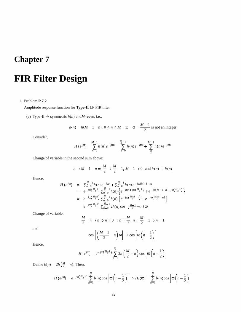
(b) Now cos�ω�n� 1
2
��can be written as a linear combination of higher harmonics in cosω multiplied by cos
�ω2
�,
i.e.,
cos
�1ω2
�= cos
ω2fcos0ωg
cos
�3ω2
�= cos
ω2f2cosω�1g
cos
�5ω2
�= cos
ω2fcos0ω�cosω+cos2ωg
etc. Note that the lowest harmonic frequency is zero and the highest harmonic frequency is(n�1)ω in thecosω
�n� 1
2
�expansion. Hence,
Hr (ω) =
M2
∑n=1
b(n)cos
�ω�
n� 12
��= cos
ω2
M2 �1
∑0
b̃(n)cos(ωn)
whereb̃(n) are related tob(n) through the above trignometric identities.
2. (Problem P 7.3) Type-III) anti-symmetrich(n) andM–odd, i.e.,
h(n) =�h(M�1�n); 0� n�M�1; h
�M�1
2
�= 0; α =
M�12
is an integer
(a) Consider,
H�ejω�= M�1
∑n=0
h(n)e� jωn =
M�32
∑n=0
h(n)e� jωn+M�1
∑M+1
2
h(n)e� jωn
Change of variable in the second sum above:
n!M�1�n) M+12
! M�32
; M�1! 0; andh(n)!�h(n)
Hence,
H�ejω� =
M�32
∑n=0
h(n)e� jωn�M�3
2
∑n=0
h(n)e� jω(M�1�n)
= e� j(M�12 )
M�32
∑n=0
h(n)n
e� jωn+ jω(M�12 )�e� jω(M�1�n)+ jω(M�1
2 )o
= e� j(M�12 )
M�32
∑n=0
h(n)n
e+ jω(M�12 �n)�e� jω(M�1
2 �n)o
= je� j(M�12 )
M�32
∑n=0
2h(n)sin
��M�1
2�n
�ω�
Change of variable:M�1
2�n! n) n= 0! n=
M�12
; n=M�3
2! n= 1
and
sin
��M�1
2�n
�ω�! sin(ωn)
Hence,
H�ejω�= je� jω(M�1
2 )M�1
2
∑n=1
2h
�M�1
2�n
�sin(ωn)
84 SOLUTIONS MANUAL FOR DSPUSING MATLAB APRIL 98
Definec(n) = 2h�
M�12 �n
�. Then,
H�ejω�= je� jω(M�1
2 )M�1
2
∑n=1
c(n)sin(ωn)) Hr (ω) =
M�12
∑n=1
c(n)sin(ωn)
(b) Now sin(ωn) can be written as a linear combination of higher harmonics in cosω multiplied by sinω, i.e.,
sin(ω) = sinωfcos0ωgsin(2ω) = sinωf2cosωgsin(3ω) = sinωfcos0ω+2cos2ωg
etc. Note that the lowest harmonic frequency is zero and the highest harmonic frequency is(n�1)ω in the sinωnexpansion. Hence,
Hr (ω) =
M�12
∑n=1
c(n)sin(ωn) = sinωM�3
2
∑0
c̃(n)cos(ωn)
wherec̃(n) are related toc(n) through the above trignometric identities.
ProblemP 7.5
MATLAB function for amplitude response:
function [Hr,w,P,L] = ampl_res(h);%% function [Hr,w,P,L] = ampl_res(h)%% Computes Amplitude response Hr(w) and its polynomial P of order L,% given a linear-phase FIR filter impulse response h.% The type of filter is determined automatically by the subroutine.%% Hr = Amplitude Response% w = frequencies between [0 pi] over which Hr is computed% P = Polynomial coefficients% L = Order of P% h = Linear Phase filter impulse response%
M = length(h);L = floor(M/2);
if fix(abs(h(1:1:L))*10ˆ10) ˜= fix(abs(h(M:-1:M-L+1))*10ˆ10)error(’Not a linear-phase impulse response’)end
if 2*L ˜= Mif fix(h(1:1:L)*10ˆ10) == fix(h(M:-1:M-L+1)*10ˆ10)disp(’*** Type-1 Linear-Phase Filter ***’)[Hr,w,P,L] = hr_type1(h);elseif fix(h(1:1:L)*10ˆ10) == -fix(h(M:-1:M-L+1)*10ˆ10)disp(’*** Type-3 Linear-Phase Filter ***’)h(L+1) = 0;[Hr,w,P,L] = hr_type3(h);endelseif fix(h(1:1:L)*10ˆ10) == fix(h(M:-1:M-L+1)*10ˆ10)disp(’*** Type-2 Linear-Phase Filter ***’)
APRIL 98 SOLUTIONS MANUAL FOR DSPUSING MATLAB 85
[Hr,w,P,L] = hr_type2(h);elseif fix(h(1:1:L)*10ˆ10) == -fix(h(M:-1:M-L+1)*10ˆ10)disp(’*** Type-4 Linear-Phase Filter ***’)[Hr,w,P,L] = hr_type4(h);endend
MATLAB verification:
clear; close all;%% Matlab verificationh1 = [1 2 3 2 1]; [Hr1,w,P1,L1] = ampl_res(h1);*** Type-1 Linear-Phase Filter ***P1, L1,P1 =
3 4 2L1 =
2%h2 = [1 2 2 1]; [Hr2,w,P2,L2] = ampl_res(h2);*** Type-2 Linear-Phase Filter ***P2, L2,P2 =
4 2L2 =
2%h3 = [1 2 0 -2 -1]; [Hr3,w,P3,L3] = ampl_res(h3);*** Type-3 Linear-Phase Filter ***P3, L3,P3 =
0 4 2L3 =
2%h4 = [1 2 -2 -1]; [Hr4,w,P4,L4] = ampl_res(h4);*** Type-4 Linear-Phase Filter ***P4, L4,P4 =
4 2L4 =
2%%% Amplitude response plotsHf_1 = figure(’Units’,’normalized’,’position’,[0.1,0.1,0.8,0.8],’color’,[0,0,0]);set(Hf_1,’NumberTitle’,’off’,’Name’,’P7.5’);
subplot(2,2,1);plot(w/pi,Hr1);title(’Type-1 FIR Filter’);ylabel(’Hr(w)’);set(gca,’XTickMode’,’manual’,’XTick’,[0:0.2:1],’fontsize’,10);
subplot(2,2,2);plot(w/pi,Hr2);title(’Type-2 FIR Filter’);ylabel(’Hr(w)’);set(gca,’XTickMode’,’manual’,’XTick’,[0:0.2:1],’fontsize’,10);
86 SOLUTIONS MANUAL FOR DSPUSING MATLAB APRIL 98
subplot(2,2,3);plot(w/pi,Hr3);title(’Type-3 FIR Filter’);ylabel(’Hr(w)’); xlabel(’frequency in pi units’);set(gca,’XTickMode’,’manual’,’XTick’,[0:0.2:1],’fontsize’,10);
subplot(2,2,4);plot(w/pi,Hr4);title(’Type-4 FIR Filter’);ylabel(’Hr(w)’); xlabel(’frequency in pi units’);set(gca,’XTickMode’,’manual’,’XTick’,[0:0.2:1],’fontsize’,10);
% Super Titlesuptitle(’Problem P7.5’);
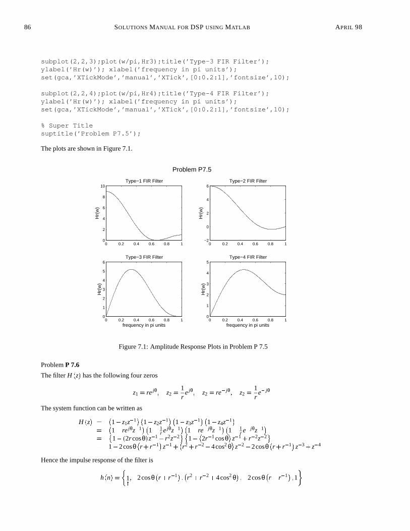
The plots are shown in Figure 7.1.
0 0.2 0.4 0.6 0.8 10
2
4
6
8
10Type−1 FIR Filter
Hr(
w)
0 0.2 0.4 0.6 0.8 1−2
0
2
4
6Type−2 FIR Filter
Hr(
w)
0 0.2 0.4 0.6 0.8 10
1
2
3
4
5
6Type−3 FIR Filter
Hr(
w)
frequency in pi units
Problem P7.5
0 0.2 0.4 0.6 0.8 10
1
2
3
4
5Type−4 FIR Filter
Hr(
w)
frequency in pi units
Figure 7.1: Amplitude Response Plots in Problem P 7.5
ProblemP 7.6
The filterH (z) has the following four zeros
z1 = rejθ; z2 =1r
ejθ; z2 = re� jθ; z2 =1r
e� jθ
The system function can be written as
H (z) =�1�z1z�1
��1�z2z�1
��1�z3z�1
��1�z4z�1
�=
�1� rejθz�1
��1� 1
r ejθz�1��
1� re� jθz�1��
1� 1r e� jθz�1
�=
�1� (2r cosθ)z�1+ r2z�2
�1��2r�1cosθ
�z�1+ r�2z�2
= 1�2cosθ
�r + r�1
�z�1+
�r2+ r�2+4cos2 θ
�z�2�2cosθ
�r + r�1
�z�3+z�4
Hence the impulse response of the filter is
h(n) =
�1";�2cosθ
�r + r�1� ;�r2+ r�2+4cos2 θ
�;�2cosθ
�r + r�1� ;1�
APRIL 98 SOLUTIONS MANUAL FOR DSPUSING MATLAB 87
which is a finite-duration symmetric impulse response. This implies that the filter is a linear-phase FIR filter.
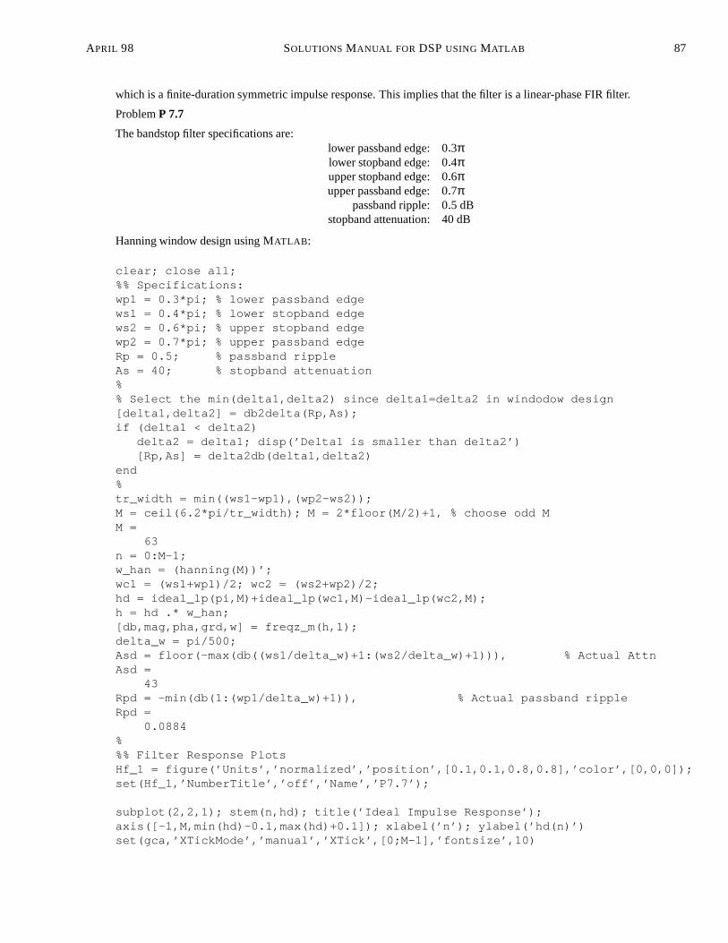
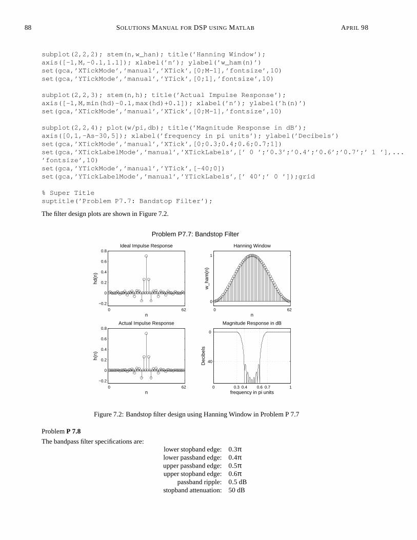
ProblemP 7.7
The bandstop filter specifications are:lower passband edge: 0:3πlower stopband edge: 0:4πupper stopband edge: 0:6πupper passband edge: 0:7π
passband ripple: 0:5 dBstopband attenuation: 40 dB
Hanning window design using MATLAB :
clear; close all;%% Specifications:wp1 = 0.3*pi; % lower passband edgews1 = 0.4*pi; % lower stopband edgews2 = 0.6*pi; % upper stopband edgewp2 = 0.7*pi; % upper passband edgeRp = 0.5; % passband rippleAs = 40; % stopband attenuation%% Select the min(delta1,delta2) since delta1=delta2 in windodow design[delta1,delta2] = db2delta(Rp,As);if (delta1 < delta2)
delta2 = delta1; disp(’Delta1 is smaller than delta2’)[Rp,As] = delta2db(delta1,delta2)
end%tr_width = min((ws1-wp1),(wp2-ws2));M = ceil(6.2*pi/tr_width); M = 2*floor(M/2)+1, % choose odd MM =
63n = 0:M-1;w_han = (hanning(M))’;wc1 = (ws1+wp1)/2; wc2 = (ws2+wp2)/2;hd = ideal_lp(pi,M)+ideal_lp(wc1,M)-ideal_lp(wc2,M);h = hd .* w_han;[db,mag,pha,grd,w] = freqz_m(h,1);delta_w = pi/500;Asd = floor(-max(db((ws1/delta_w)+1:(ws2/delta_w)+1))), % Actual AttnAsd =
43Rpd = -min(db(1:(wp1/delta_w)+1)), % Actual passband rippleRpd =
0.0884%%% Filter Response PlotsHf_1 = figure(’Units’,’normalized’,’position’,[0.1,0.1,0.8,0.8],’color’,[0,0,0]);set(Hf_1,’NumberTitle’,’off’,’Name’,’P7.7’);
subplot(2,2,1); stem(n,hd); title(’Ideal Impulse Response’);axis([-1,M,min(hd)-0.1,max(hd)+0.1]); xlabel(’n’); ylabel(’hd(n)’)set(gca,’XTickMode’,’manual’,’XTick’,[0;M-1],’fontsize’,10)
88 SOLUTIONS MANUAL FOR DSPUSING MATLAB APRIL 98
subplot(2,2,2); stem(n,w_han); title(’Hanning Window’);axis([-1,M,-0.1,1.1]); xlabel(’n’); ylabel(’w_ham(n)’)set(gca,’XTickMode’,’manual’,’XTick’,[0;M-1],’fontsize’,10)set(gca,’YTickMode’,’manual’,’YTick’,[0;1],’fontsize’,10)
subplot(2,2,3); stem(n,h); title(’Actual Impulse Response’);axis([-1,M,min(hd)-0.1,max(hd)+0.1]); xlabel(’n’); ylabel(’h(n)’)set(gca,’XTickMode’,’manual’,’XTick’,[0;M-1],’fontsize’,10)
subplot(2,2,4); plot(w/pi,db); title(’Magnitude Response in dB’);axis([0,1,-As-30,5]); xlabel(’frequency in pi units’); ylabel(’Decibels’)set(gca,’XTickMode’,’manual’,’XTick’,[0;0.3;0.4;0.6;0.7;1])set(gca,’XTickLabelMode’,’manual’,’XTickLabels’,[’ 0 ’;’0.3’;’0.4’;’0.6’;’0.7’;’ 1 ’],...’fontsize’,10)set(gca,’YTickMode’,’manual’,’YTick’,[-40;0])set(gca,’YTickLabelMode’,’manual’,’YTickLabels’,[’ 40’;’ 0 ’]);grid
% Super Titlesuptitle(’Problem P7.7: Bandstop Filter’);
The filter design plots are shown in Figure 7.2.
0 62
−0.2
0
0.2
0.4
0.6
0.8
n
hd(n
)
Ideal Impulse Response
0 62
0
1
n
w_h
am(n
)
Hanning Window
0 62
−0.2
0
0.2
0.4
0.6
0.8
n
h(n)
Actual Impulse Response
Problem P7.7: Bandstop Filter
0 0.3 0.4 0.6 0.7 1
40
0
Magnitude Response in dB
frequency in pi units
Dec
ibel
s
Figure 7.2: Bandstop filter design using Hanning Window in Problem P 7.7
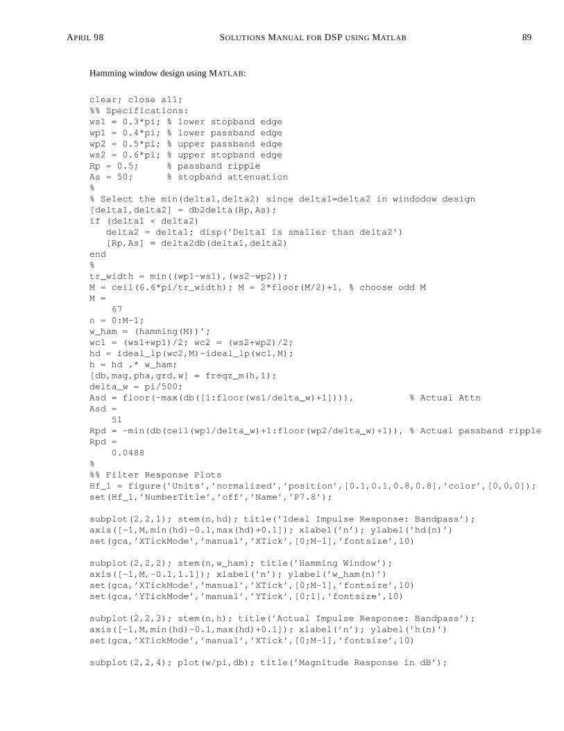
ProblemP 7.8
The bandpass filter specifications are:lower stopband edge: 0:3πlower passband edge: 0:4πupper passband edge: 0:5πupper stopband edge: 0:6π
passband ripple: 0:5 dBstopband attenuation: 50 dB
APRIL 98 SOLUTIONS MANUAL FOR DSPUSING MATLAB 89
Hamming window design using MATLAB :
clear; close all;%% Specifications:ws1 = 0.3*pi; % lower stopband edgewp1 = 0.4*pi; % lower passband edgewp2 = 0.5*pi; % upper passband edgews2 = 0.6*pi; % upper stopband edgeRp = 0.5; % passband rippleAs = 50; % stopband attenuation%% Select the min(delta1,delta2) since delta1=delta2 in windodow design[delta1,delta2] = db2delta(Rp,As);if (delta1 < delta2)
delta2 = delta1; disp(’Delta1 is smaller than delta2’)[Rp,As] = delta2db(delta1,delta2)
end%tr_width = min((wp1-ws1),(ws2-wp2));M = ceil(6.6*pi/tr_width); M = 2*floor(M/2)+1, % choose odd MM =
67n = 0:M-1;w_ham = (hamming(M))’;wc1 = (ws1+wp1)/2; wc2 = (ws2+wp2)/2;hd = ideal_lp(wc2,M)-ideal_lp(wc1,M);h = hd .* w_ham;[db,mag,pha,grd,w] = freqz_m(h,1);delta_w = pi/500;Asd = floor(-max(db([1:floor(ws1/delta_w)+1]))), % Actual AttnAsd =
51Rpd = -min(db(ceil(wp1/delta_w)+1:floor(wp2/delta_w)+1)), % Actual passband rippleRpd =
0.0488%%% Filter Response PlotsHf_1 = figure(’Units’,’normalized’,’position’,[0.1,0.1,0.8,0.8],’color’,[0,0,0]);set(Hf_1,’NumberTitle’,’off’,’Name’,’P7.8’);
subplot(2,2,1); stem(n,hd); title(’Ideal Impulse Response: Bandpass’);axis([-1,M,min(hd)-0.1,max(hd)+0.1]); xlabel(’n’); ylabel(’hd(n)’)set(gca,’XTickMode’,’manual’,’XTick’,[0;M-1],’fontsize’,10)
subplot(2,2,2); stem(n,w_ham); title(’Hamming Window’);axis([-1,M,-0.1,1.1]); xlabel(’n’); ylabel(’w_ham(n)’)set(gca,’XTickMode’,’manual’,’XTick’,[0;M-1],’fontsize’,10)set(gca,’YTickMode’,’manual’,’YTick’,[0;1],’fontsize’,10)
subplot(2,2,3); stem(n,h); title(’Actual Impulse Response: Bandpass’);axis([-1,M,min(hd)-0.1,max(hd)+0.1]); xlabel(’n’); ylabel(’h(n)’)set(gca,’XTickMode’,’manual’,’XTick’,[0;M-1],’fontsize’,10)
subplot(2,2,4); plot(w/pi,db); title(’Magnitude Response in dB’);
90 SOLUTIONS MANUAL FOR DSPUSING MATLAB APRIL 98
axis([0,1,-As-30,5]); xlabel(’frequency in pi units’); ylabel(’Decibels’)set(gca,’XTickMode’,’manual’,’XTick’,[0;0.3;0.4;0.5;0.6;1])set(gca,’XTickLabelMode’,’manual’,’XTickLabels’,[’ 0 ’;’0.3’;’0.4’;’0.5’;’0.6’;’ 1 ’],...’fontsize’,10)set(gca,’YTickMode’,’manual’,’YTick’,[-50;0])set(gca,’YTickLabelMode’,’manual’,’YTickLabels’,[’-50’;’ 0 ’]);grid
The filter design plots are shown in Figure 7.3.
0 66
−0.2
−0.1
0
0.1
0.2
0.3
n
hd(n
)
Ideal Impulse Response: Bandpass
0 66
0
1
n
w_h
am(n
)
Hamming Window
0 66
−0.2
−0.1
0
0.1
0.2
0.3
n
h(n)
Actual Impulse Response: Bandpass
Homework−4 : Problem 3
0 0.3 0.4 0.5 0.6 1
−50
0
Magnitude Response in dB
frequency in pi units
Dec
ibel
s
Figure 7.3: Bandpass filter design using Hamming Window in Problem P 7.8
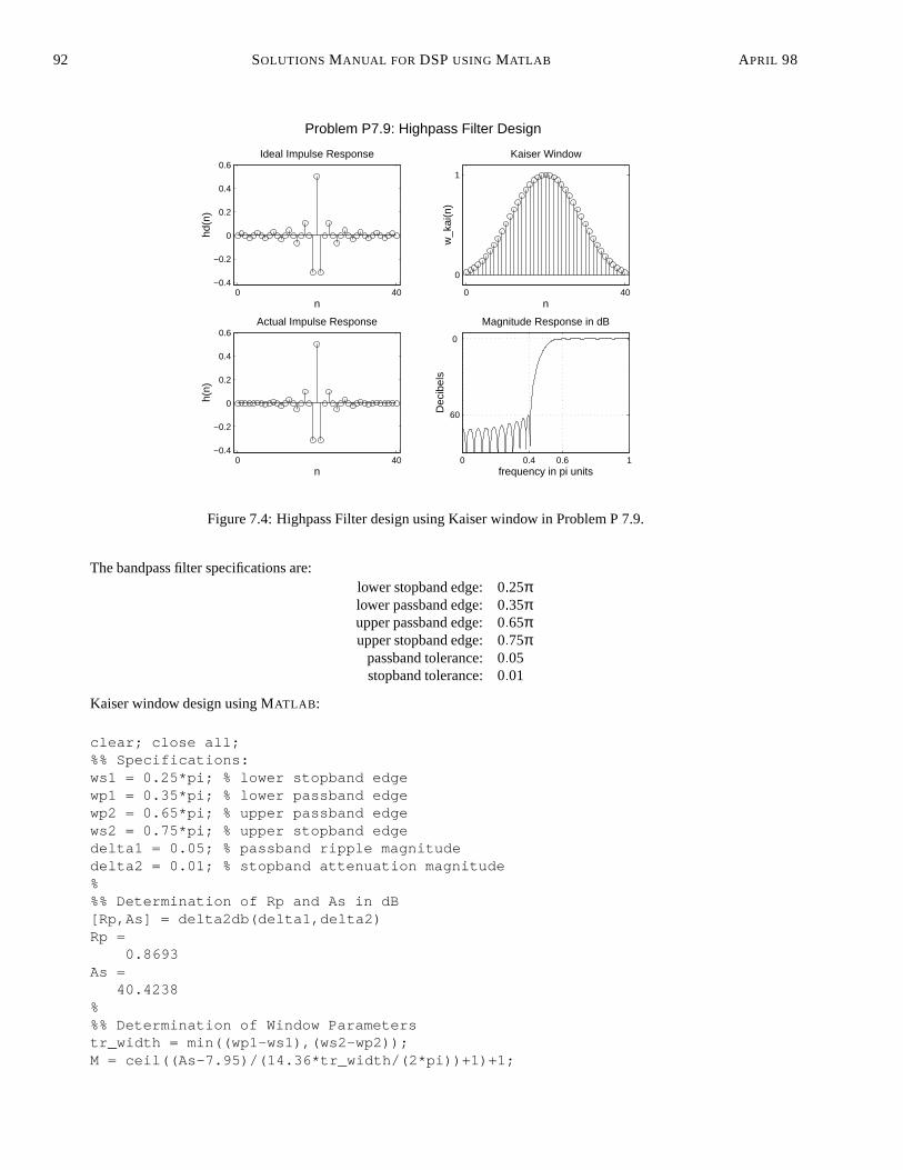
3. (Problem P 7.9) The highpass filter specifications are:
stopband edge: 0:4πpassband edge: 0:6π
passband ripple: 0:5 dBstopband attenuation: 60 dB
Kaiser window design using MATLAB :
clear; close all;%% Specifications:ws = 0.4*pi; % stopband edgewp = 0.6*pi; % passband edgeRp = 0.5; % passband rippleAs = 60; % stopband attenuation%% Select the min(delta1,delta2) since delta1=delta2 in windodow design[delta1,delta2] = db2delta(Rp,As);if (delta1 < delta2)
delta2 = delta1; disp(’Delta1 is smaller than delta2’)
APRIL 98 SOLUTIONS MANUAL FOR DSPUSING MATLAB 91
[Rp,As] = delta2db(delta1,delta2)end%tr_width = wp-ws; M = ceil((As-7.95)/(14.36*tr_width/(2*pi))+1)+1;M = 2*floor(M/2)+3, % choose odd M, Increased order by 2 to get Asd>60M =
41n = [0:1:M-1]; beta = 0.1102*(As-8.7);w_kai = (kaiser(M,beta))’; % Kaiser Windowwc = (ws+wp)/2; hd = ideal_lp(pi,M)-ideal_lp(wc,M); % Ideal HP Filterh = hd .* w_kai; % Window design[db,mag,pha,grd,w] = freqz_m(h,1);delta_w = pi/500;Asd = -floor(max(db(1:1:(ws/delta_w)+1))), % Actual AttnAsd =
61Rpd = -min(db((wp/delta_w)+1:1:501)), % Actual passband rippleRpd =
0.0148%%% Filter Response PlotsHf_1 = figure(’Units’,’normalized’,’position’,[0.1,0.1,0.8,0.8],’color’,[0,0,0]);set(Hf_1,’NumberTitle’,’off’,’Name’,’P7.9’);
subplot(2,2,1); stem(n,hd); title(’Ideal Impulse Response’);axis([-1,M,min(hd)-0.1,max(hd)+0.1]); xlabel(’n’); ylabel(’hd(n)’)set(gca,’XTickMode’,’manual’,’XTick’,[0;M-1],’fontsize’,10)
subplot(2,2,2); stem(n,w_kai); title(’Kaiser Window’);axis([-1,M,-0.1,1.1]); xlabel(’n’); ylabel(’w_kai(n)’)set(gca,’XTickMode’,’manual’,’XTick’,[0;M-1],’fontsize’,10)set(gca,’YTickMode’,’manual’,’YTick’,[0;1],’fontsize’,10)
subplot(2,2,3); stem(n,h); title(’Actual Impulse Response’);axis([-1,M,min(hd)-0.1,max(hd)+0.1]); xlabel(’n’); ylabel(’h(n)’)set(gca,’XTickMode’,’manual’,’XTick’,[0;M-1],’fontsize’,10)
subplot(2,2,4); plot(w/pi,db); title(’Magnitude Response in dB’);axis([0,1,-As-30,5]); xlabel(’frequency in pi units’); ylabel(’Decibels’)set(gca,’XTickMode’,’manual’,’XTick’,[0;0.4;0.6;1])set(gca,’XTickLabelMode’,’manual’,’XTickLabels’,[’ 0 ’;’0.4’;’0.6’;’ 1 ’],...’fontsize’,10)set(gca,’YTickMode’,’manual’,’YTick’,[-60;0])set(gca,’YTickLabelMode’,’manual’,’YTickLabels’,[’ 60’;’ 0 ’]);grid
% Super Titlesuptitle(’Problem P7.9: Highpass Filter Design’);
The filter design plots are shown in Figure 7.4.
ProblemP 7.10
92 SOLUTIONS MANUAL FOR DSPUSING MATLAB APRIL 98
0 40−0.4
−0.2
0
0.2
0.4
0.6
n
hd(n
)
Ideal Impulse Response
0 40
0
1
n
w_k
ai(n
)
Kaiser Window
0 40−0.4
−0.2
0
0.2
0.4
0.6
n
h(n)
Actual Impulse Response
Problem P7.9: Highpass Filter Design
0 0.4 0.6 1
60
0
Magnitude Response in dB
frequency in pi units
Dec
ibel
s
Figure 7.4: Highpass Filter design using Kaiser window in Problem P 7.9.
The bandpass filter specifications are:lower stopband edge: 0:25πlower passband edge: 0:35πupper passband edge: 0:65πupper stopband edge: 0:75π
passband tolerance: 0:05stopband tolerance: 0:01
Kaiser window design using MATLAB :
clear; close all;%% Specifications:ws1 = 0.25*pi; % lower stopband edgewp1 = 0.35*pi; % lower passband edgewp2 = 0.65*pi; % upper passband edgews2 = 0.75*pi; % upper stopband edgedelta1 = 0.05; % passband ripple magnitudedelta2 = 0.01; % stopband attenuation magnitude%%% Determination of Rp and As in dB[Rp,As] = delta2db(delta1,delta2)Rp =
0.8693As =
40.4238%%% Determination of Window Parameterstr_width = min((wp1-ws1),(ws2-wp2));M = ceil((As-7.95)/(14.36*tr_width/(2*pi))+1)+1;
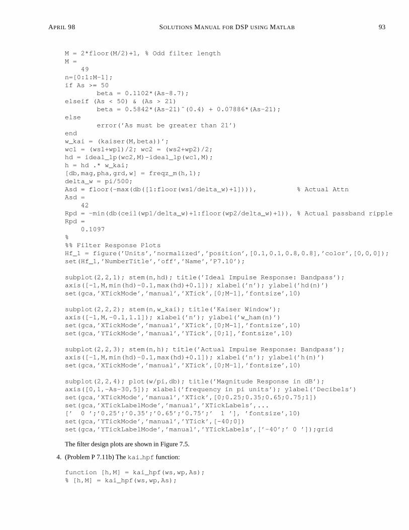
APRIL 98 SOLUTIONS MANUAL FOR DSPUSING MATLAB 93
M = 2*floor(M/2)+1, % Odd filter lengthM =
49n=[0:1:M-1];if As >= 50
beta = 0.1102*(As-8.7);elseif (As < 50) & (As > 21)
beta = 0.5842*(As-21)ˆ(0.4) + 0.07886*(As-21);else
error(’As must be greater than 21’)endw_kai = (kaiser(M,beta))’;wc1 = (ws1+wp1)/2; wc2 = (ws2+wp2)/2;hd = ideal_lp(wc2,M)-ideal_lp(wc1,M);h = hd .* w_kai;[db,mag,pha,grd,w] = freqz_m(h,1);delta_w = pi/500;Asd = floor(-max(db([1:floor(ws1/delta_w)+1]))), % Actual AttnAsd =
42Rpd = -min(db(ceil(wp1/delta_w)+1:floor(wp2/delta_w)+1)), % Actual passband rippleRpd =
0.1097%%% Filter Response PlotsHf_1 = figure(’Units’,’normalized’,’position’,[0.1,0.1,0.8,0.8],’color’,[0,0,0]);set(Hf_1,’NumberTitle’,’off’,’Name’,’P7.10’);
subplot(2,2,1); stem(n,hd); title(’Ideal Impulse Response: Bandpass’);axis([-1,M,min(hd)-0.1,max(hd)+0.1]); xlabel(’n’); ylabel(’hd(n)’)set(gca,’XTickMode’,’manual’,’XTick’,[0;M-1],’fontsize’,10)
subplot(2,2,2); stem(n,w_kai); title(’Kaiser Window’);axis([-1,M,-0.1,1.1]); xlabel(’n’); ylabel(’w_ham(n)’)set(gca,’XTickMode’,’manual’,’XTick’,[0;M-1],’fontsize’,10)set(gca,’YTickMode’,’manual’,’YTick’,[0;1],’fontsize’,10)
subplot(2,2,3); stem(n,h); title(’Actual Impulse Response: Bandpass’);axis([-1,M,min(hd)-0.1,max(hd)+0.1]); xlabel(’n’); ylabel(’h(n)’)set(gca,’XTickMode’,’manual’,’XTick’,[0;M-1],’fontsize’,10)
subplot(2,2,4); plot(w/pi,db); title(’Magnitude Response in dB’);axis([0,1,-As-30,5]); xlabel(’frequency in pi units’); ylabel(’Decibels’)set(gca,’XTickMode’,’manual’,’XTick’,[0;0.25;0.35;0.65;0.75;1])set(gca,’XTickLabelMode’,’manual’,’XTickLabels’,...[’ 0 ’;’0.25’;’0.35’;’0.65’;’0.75’;’ 1 ’], ’fontsize’,10)set(gca,’YTickMode’,’manual’,’YTick’,[-40;0])set(gca,’YTickLabelMode’,’manual’,’YTickLabels’,[’-40’;’ 0 ’]);grid
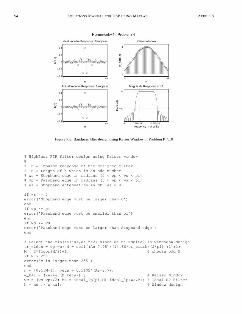
The filter design plots are shown in Figure 7.5.
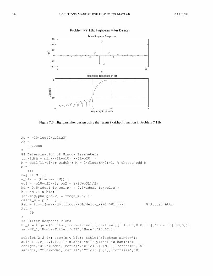
4. (Problem P 7.11b) Thekai hpf function:
function [h,M] = kai_hpf(ws,wp,As);% [h,M] = kai_hpf(ws,wp,As);
94 SOLUTIONS MANUAL FOR DSPUSING MATLAB APRIL 98
0 48−0.4
−0.2
0
0.2
0.4
n
hd(n
)
Ideal Impulse Response: Bandpass
0 48
0
1
n
w_h
am(n
)
Kaiser Window
0 48−0.4
−0.2
0
0.2
0.4
n
h(n)
Actual Impulse Response: Bandpass
Homework−4 : Problem 4
0 0.250.35 0.650.75 1
−40
0
Magnitude Response in dB
frequency in pi units
Dec
ibel
s
Figure 7.5: Bandpass filter design using Kaiser Window in Problem P 7.10
% HighPass FIR filter design using Kaiser window%% h = Impulse response of the designed filter% M = Length of h which is an odd number% ws = Stopband edge in radians (0 < wp < ws < pi)% wp = Passband edge in radians (0 < wp < ws < pi)% As = Stopband attenuation in dB (As > 0)
if ws <= 0error(’Stopband edge must be larger than 0’)endif wp >= pierror(’Passband edge must be smaller than pi’)endif wp <= wserror(’Passband edge must be larger than Stopband edge’)end
% Select the min(delta1,delta2) since delta1=delta2 in windodow designtr_width = wp-ws; M = ceil((As-7.95)/(14.36*tr_width/(2*pi))+1)+1;M = 2*floor(M/2)+1; % choose odd Mif M > 255error(’M is larger than 255’)endn = [0:1:M-1]; beta = 0.1102*(As-8.7);w_kai = (kaiser(M,beta))’; % Kaiser Windowwc = (ws+wp)/2; hd = ideal_lp(pi,M)-ideal_lp(wc,M); % Ideal HP Filterh = hd .* w_kai; % Window design
APRIL 98 SOLUTIONS MANUAL FOR DSPUSING MATLAB 95
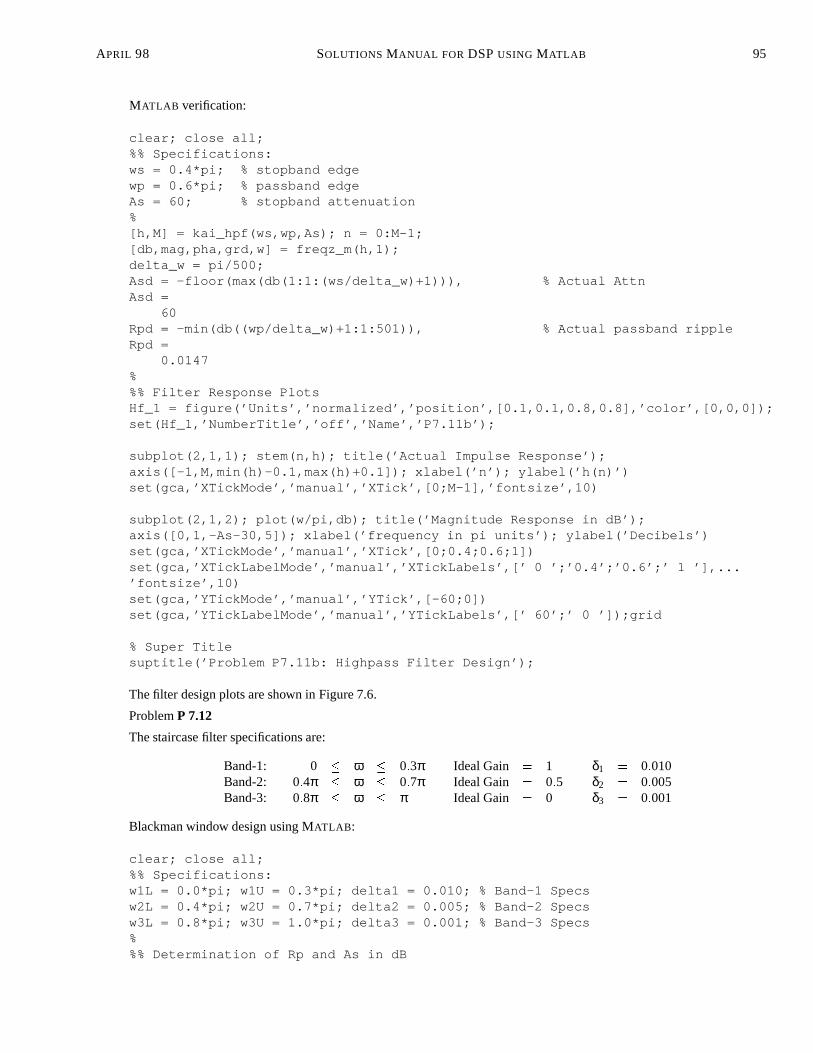
MATLAB verification:
clear; close all;%% Specifications:ws = 0.4*pi; % stopband edgewp = 0.6*pi; % passband edgeAs = 60; % stopband attenuation%[h,M] = kai_hpf(ws,wp,As); n = 0:M-1;[db,mag,pha,grd,w] = freqz_m(h,1);delta_w = pi/500;Asd = -floor(max(db(1:1:(ws/delta_w)+1))), % Actual AttnAsd =
60Rpd = -min(db((wp/delta_w)+1:1:501)), % Actual passband rippleRpd =
0.0147%%% Filter Response PlotsHf_1 = figure(’Units’,’normalized’,’position’,[0.1,0.1,0.8,0.8],’color’,[0,0,0]);set(Hf_1,’NumberTitle’,’off’,’Name’,’P7.11b’);
subplot(2,1,1); stem(n,h); title(’Actual Impulse Response’);axis([-1,M,min(h)-0.1,max(h)+0.1]); xlabel(’n’); ylabel(’h(n)’)set(gca,’XTickMode’,’manual’,’XTick’,[0;M-1],’fontsize’,10)
subplot(2,1,2); plot(w/pi,db); title(’Magnitude Response in dB’);axis([0,1,-As-30,5]); xlabel(’frequency in pi units’); ylabel(’Decibels’)set(gca,’XTickMode’,’manual’,’XTick’,[0;0.4;0.6;1])set(gca,’XTickLabelMode’,’manual’,’XTickLabels’,[’ 0 ’;’0.4’;’0.6’;’ 1 ’],...’fontsize’,10)set(gca,’YTickMode’,’manual’,’YTick’,[-60;0])set(gca,’YTickLabelMode’,’manual’,’YTickLabels’,[’ 60’;’ 0 ’]);grid
% Super Titlesuptitle(’Problem P7.11b: Highpass Filter Design’);
The filter design plots are shown in Figure 7.6.
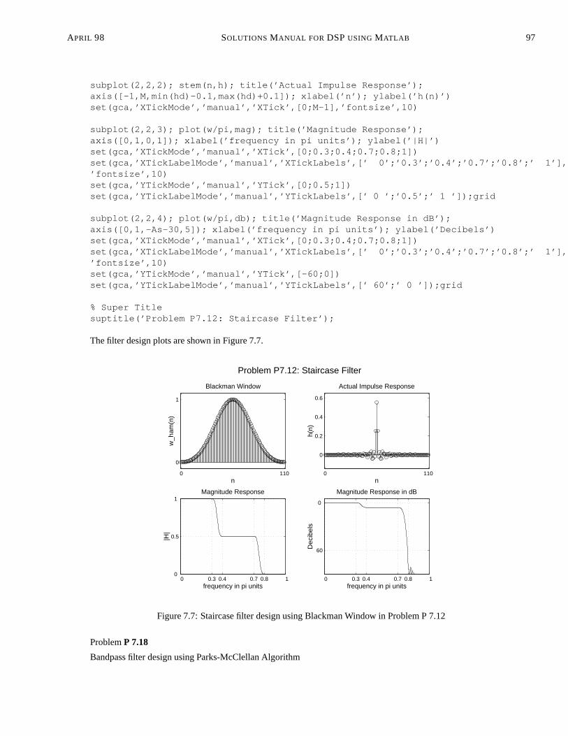
ProblemP 7.12
The staircase filter specifications are:
Band-1:Band-2:Band-3:
0 � ω � 0:3π0:4π � ω � 0:7π0:8π � ω � π
Ideal Gain = 1Ideal Gain = 0:5Ideal Gain = 0
δ1 = 0:010δ2 = 0:005δ3 = 0:001
Blackman window design using MATLAB :
clear; close all;%% Specifications:w1L = 0.0*pi; w1U = 0.3*pi; delta1 = 0.010; % Band-1 Specsw2L = 0.4*pi; w2U = 0.7*pi; delta2 = 0.005; % Band-2 Specsw3L = 0.8*pi; w3U = 1.0*pi; delta3 = 0.001; % Band-3 Specs%%% Determination of Rp and As in dB
96 SOLUTIONS MANUAL FOR DSPUSING MATLAB APRIL 98
0 38−0.4
−0.2
0
0.2
0.4
0.6
n
h(n)
Actual Impulse Response
Problem P7.11b: Highpass Filter Design
0 0.4 0.6 1
60
0
Magnitude Response in dB
frequency in pi units
Dec
ibel
s
Figure 7.6: Highpass filter design using thentextttfkai hpfg function in Problem 7.11b.
As = -20*log10(delta3)As =
60.0000%%% Determination of Window Parameterstr_width = min((w2L-w1U),(w3L-w2U));M = ceil(11*pi/tr_width); M = 2*floor(M/2)+1, % choose odd MM =
111n=[0:1:M-1];w_bla = (blackman(M))’;wc1 = (w1U+w2L)/2; wc2 = (w2U+w3L)/2;hd = 0.5*ideal_lp(wc1,M) + 0.5*ideal_lp(wc2,M);h = hd .* w_bla;[db,mag,pha,grd,w] = freqz_m(h,1);delta_w = pi/500;Asd = floor(-max(db([floor(w3L/delta_w)+1:501]))), % Actual AttnAsd =
79%%% Filter Response PlotsHf_1 = figure(’Units’,’normalized’,’position’,[0.1,0.1,0.8,0.8],’color’,[0,0,0]);set(Hf_1,’NumberTitle’,’off’,’Name’,’P7.12’);
subplot(2,2,1); stem(n,w_bla); title(’Blackman Window’);axis([-1,M,-0.1,1.1]); xlabel(’n’); ylabel(’w_ham(n)’)set(gca,’XTickMode’,’manual’,’XTick’,[0;M-1],’fontsize’,10)set(gca,’YTickMode’,’manual’,’YTick’,[0;1],’fontsize’,10)
APRIL 98 SOLUTIONS MANUAL FOR DSPUSING MATLAB 97
subplot(2,2,2); stem(n,h); title(’Actual Impulse Response’);axis([-1,M,min(hd)-0.1,max(hd)+0.1]); xlabel(’n’); ylabel(’h(n)’)set(gca,’XTickMode’,’manual’,’XTick’,[0;M-1],’fontsize’,10)
subplot(2,2,3); plot(w/pi,mag); title(’Magnitude Response’);axis([0,1,0,1]); xlabel(’frequency in pi units’); ylabel(’|H|’)set(gca,’XTickMode’,’manual’,’XTick’,[0;0.3;0.4;0.7;0.8;1])set(gca,’XTickLabelMode’,’manual’,’XTickLabels’,[’ 0’;’0.3’;’0.4’;’0.7’;’0.8’;’ 1’],’fontsize’,10)set(gca,’YTickMode’,’manual’,’YTick’,[0;0.5;1])set(gca,’YTickLabelMode’,’manual’,’YTickLabels’,[’ 0 ’;’0.5’;’ 1 ’]);grid
subplot(2,2,4); plot(w/pi,db); title(’Magnitude Response in dB’);axis([0,1,-As-30,5]); xlabel(’frequency in pi units’); ylabel(’Decibels’)set(gca,’XTickMode’,’manual’,’XTick’,[0;0.3;0.4;0.7;0.8;1])set(gca,’XTickLabelMode’,’manual’,’XTickLabels’,[’ 0’;’0.3’;’0.4’;’0.7’;’0.8’;’ 1’],’fontsize’,10)set(gca,’YTickMode’,’manual’,’YTick’,[-60;0])set(gca,’YTickLabelMode’,’manual’,’YTickLabels’,[’ 60’;’ 0 ’]);grid
% Super Titlesuptitle(’Problem P7.12: Staircase Filter’);
The filter design plots are shown in Figure 7.7.
0 110
0
1
n
w_h
am(n
)
Blackman Window
0 110
0
0.2
0.4
0.6
n
h(n)
Actual Impulse Response
0 0.3 0.4 0.7 0.8 1 0
0.5
1 Magnitude Response
frequency in pi units
|H|
Problem P7.12: Staircase Filter
0 0.3 0.4 0.7 0.8 1
60
0
Magnitude Response in dB
frequency in pi units
Dec
ibel
s
Figure 7.7: Staircase filter design using Blackman Window in Problem P 7.12
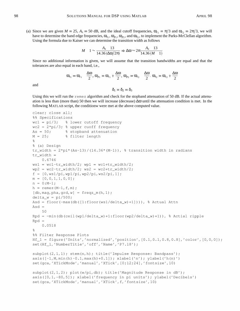
ProblemP 7.18
Bandpass filter design using Parks-McClellan Algorithm
98 SOLUTIONS MANUAL FOR DSPUSING MATLAB APRIL 98
(a) Since we are givenM = 25, As = 50 dB, and the ideal cutoff frequencies,ωc1 = π=3 andωc2 = 2π=3, we willhave to determine the band edge frequencies,ωs1, ωp1, ωp2, andωS2, to implement the Parks-McClellan algorithm.Using the formula due to Kaiser we can determine the transition width as follows
M�1' As�1314:36(∆ω=2π)
) ∆ω' 2πAs�13
14:36(M�1)
Since no additional information is given, we will assume that the transition bandwidths are equal and that thetolerances are also equal in each band, i.e.,
ωs1 = ωc1�∆ω2
; ωp1 = ωc1 +∆ω2
; ωp2 = ωc2�∆ω2
; ωs2 = ωc2 +∆ω2
andδ1 = δ2 = δ3
Using this we will run theremez algorithm and check for the stopband attenuation of 50 dB. If the actual attenu-ation is less than (more than) 50 then we will increase (decrease)∆ω until the attenuation condition is met. In thefollowing MATLAB script, the conditionw were met at the above computed value.
clear; close all;%% Specificationswc1 = pi/3; % lower cutoff frequencywc2 = 2*pi/3; % upper cuoff frequencyAs = 50; % stopband attenuationM = 25; % filter length%% (a) Designtr_width = 2*pi*(As-13)/(14.36*(M-1)), % transition width in radianstr_width =
0.6746ws1 = wc1-tr_width/2; wp1 = wc1+tr_width/2;wp2 = wc2-tr_width/2; ws2 = wc2+tr_width/2;f = [0,ws1/pi,wp1/pi,wp2/pi,ws2/pi,1];m = [0,0,1,1,0,0];n = 0:M-1;h = remez(M-1,f,m);[db,mag,pha,grd,w] = freqz_m(h,1);delta_w = pi/500;Asd = floor(-max(db([1:floor(ws1/delta_w)+1]))), % Actual AttnAsd =
50Rpd = -min(db(ceil(wp1/delta_w)+1:floor(wp2/delta_w)+1)), % Actial rippleRpd =
0.0518%%% Filter Response PlotsHf_1 = figure(’Units’,’normalized’,’position’,[0.1,0.1,0.8,0.8],’color’,[0,0,0]);set(Hf_1,’NumberTitle’,’off’,’Name’,’P7.18’);
subplot(2,1,1); stem(n,h); title(’Impulse Response: Bandpass’);axis([-1,M,min(h)-0.1,max(h)+0.1]); xlabel(’n’); ylabel(’h(n)’)set(gca,’XTickMode’,’manual’,’XTick’,[0;12;24],’fontsize’,10)
subplot(2,1,2); plot(w/pi,db); title(’Magnitude Response in dB’);axis([0,1,-80,5]); xlabel(’frequency in pi units’); ylabel(’Decibels’)set(gca,’XTickMode’,’manual’,’XTick’,f,’fontsize’,10)
APRIL 98 SOLUTIONS MANUAL FOR DSPUSING MATLAB 99
set(gca,’YTickMode’,’manual’,’YTick’,[-50;0])set(gca,’YTickLabelMode’,’manual’,’YTickLabels’,[’-50’;’ 0 ’],’fontsize’,10);grid
The impulse response plot is shown in Figure 7.8.
0 12 24
−0.2
0
0.2
0.4
n
h(n)
Impulse Response: Bandpass
Homework−4 : Problem 5a
0 0.226 0.4407 0.5593 0.774 1
−50
0
Magnitude Response in dB
frequency in pi units
Dec
ibel
s
Figure 7.8: Impulse Response Plot in Problem P 7.18
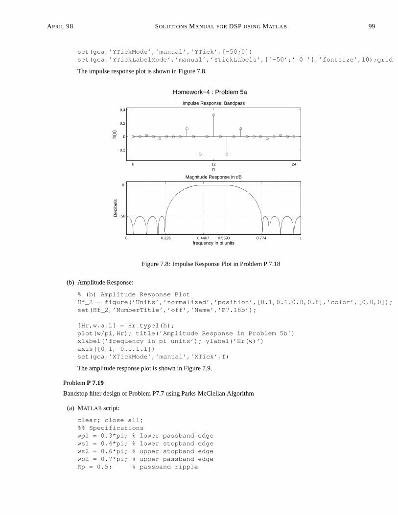
(b) Amplitude Response:
% (b) Amplitude Response PlotHf_2 = figure(’Units’,’normalized’,’position’,[0.1,0.1,0.8,0.8],’color’,[0,0,0]);set(Hf_2,’NumberTitle’,’off’,’Name’,’P7.18b’);
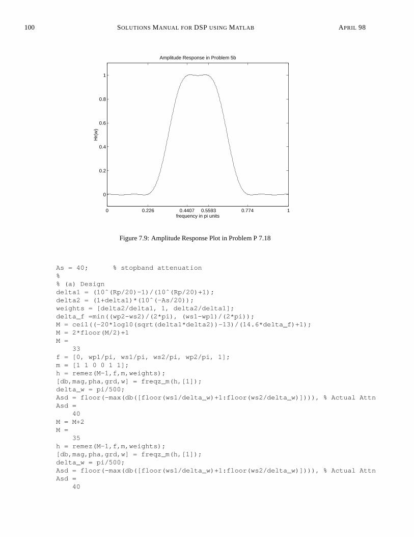
[Hr,w,a,L] = Hr_type1(h);plot(w/pi,Hr); title(’Amplitude Response in Problem 5b’)xlabel(’frequency in pi units’); ylabel(’Hr(w)’)axis([0,1,-0.1,1.1])set(gca,’XTickMode’,’manual’,’XTick’,f)
The amplitude response plot is shown in Figure 7.9.
ProblemP 7.19
Bandstop filter design of Problem P7.7 using Parks-McClellan Algorithm
(a) MATLAB script:
clear; close all;%% Specificationswp1 = 0.3*pi; % lower passband edgews1 = 0.4*pi; % lower stopband edgews2 = 0.6*pi; % upper stopband edgewp2 = 0.7*pi; % upper passband edgeRp = 0.5; % passband ripple
100 SOLUTIONS MANUAL FOR DSPUSING MATLAB APRIL 98
0 0.226 0.4407 0.5593 0.774 1
0
0.2
0.4
0.6
0.8
1
Amplitude Response in Problem 5b
frequency in pi units
Hr(
w)
Figure 7.9: Amplitude Response Plot in Problem P 7.18
As = 40; % stopband attenuation%% (a) Designdelta1 = (10ˆ(Rp/20)-1)/(10ˆ(Rp/20)+1);delta2 = (1+delta1)*(10ˆ(-As/20));weights = [delta2/delta1, 1, delta2/delta1];delta_f =min((wp2-ws2)/(2*pi), (ws1-wp1)/(2*pi));M = ceil((-20*log10(sqrt(delta1*delta2))-13)/(14.6*delta_f)+1);M = 2*floor(M/2)+1M =
33f = [0, wp1/pi, ws1/pi, ws2/pi, wp2/pi, 1];m = [1 1 0 0 1 1];h = remez(M-1,f,m,weights);[db,mag,pha,grd,w] = freqz_m(h,[1]);delta_w = pi/500;Asd = floor(-max(db([floor(ws1/delta_w)+1:floor(ws2/delta_w)]))), % Actual AttnAsd =
40M = M+2M =
35h = remez(M-1,f,m,weights);[db,mag,pha,grd,w] = freqz_m(h,[1]);delta_w = pi/500;Asd = floor(-max(db([floor(ws1/delta_w)+1:floor(ws2/delta_w)]))), % Actual AttnAsd =
40
APRIL 98 SOLUTIONS MANUAL FOR DSPUSING MATLAB 101
n = 0:M-1;%%%Filter Response PlotsHf_1 = figure(’Units’,’normalized’,’position’,[0.1,0.1,0.8,0.8],’color’,[0,0,0]);set(Hf_1,’NumberTitle’,’off’,’Name’,’P7.19a’);
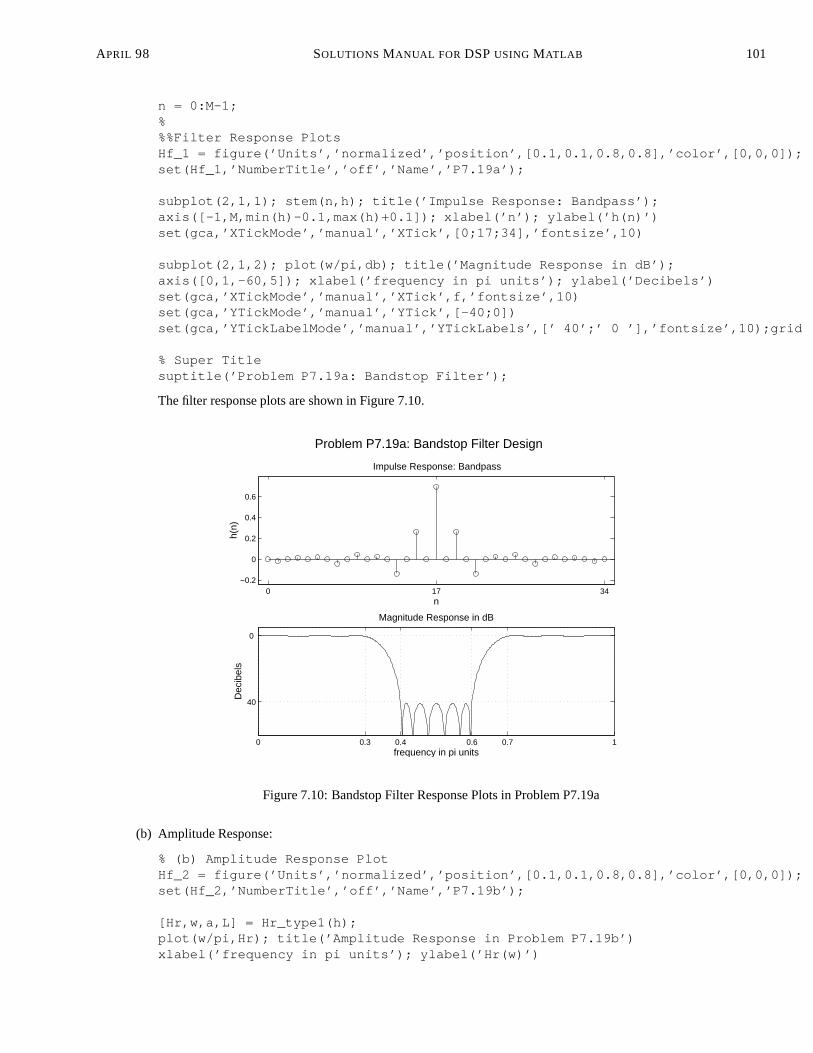
subplot(2,1,1); stem(n,h); title(’Impulse Response: Bandpass’);axis([-1,M,min(h)-0.1,max(h)+0.1]); xlabel(’n’); ylabel(’h(n)’)set(gca,’XTickMode’,’manual’,’XTick’,[0;17;34],’fontsize’,10)
subplot(2,1,2); plot(w/pi,db); title(’Magnitude Response in dB’);axis([0,1,-60,5]); xlabel(’frequency in pi units’); ylabel(’Decibels’)set(gca,’XTickMode’,’manual’,’XTick’,f,’fontsize’,10)set(gca,’YTickMode’,’manual’,’YTick’,[-40;0])set(gca,’YTickLabelMode’,’manual’,’YTickLabels’,[’ 40’;’ 0 ’],’fontsize’,10);grid
% Super Titlesuptitle(’Problem P7.19a: Bandstop Filter’);
The filter response plots are shown in Figure 7.10.
0 17 34−0.2
0
0.2
0.4
0.6
n
h(n)
Impulse Response: Bandpass
Problem P7.19a: Bandstop Filter Design
0 0.3 0.4 0.6 0.7 1
40
0
Magnitude Response in dB
frequency in pi units
Dec
ibel
s
Figure 7.10: Bandstop Filter Response Plots in Problem P7.19a
(b) Amplitude Response:
% (b) Amplitude Response PlotHf_2 = figure(’Units’,’normalized’,’position’,[0.1,0.1,0.8,0.8],’color’,[0,0,0]);set(Hf_2,’NumberTitle’,’off’,’Name’,’P7.19b’);
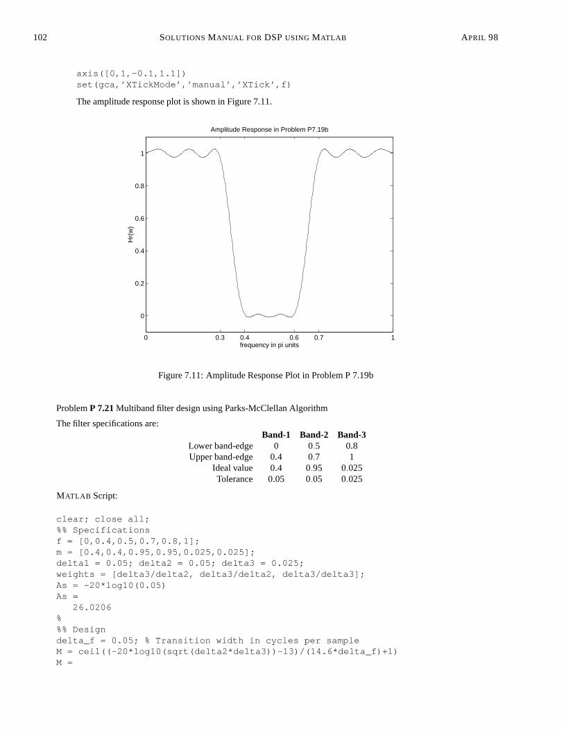
[Hr,w,a,L] = Hr_type1(h);plot(w/pi,Hr); title(’Amplitude Response in Problem P7.19b’)xlabel(’frequency in pi units’); ylabel(’Hr(w)’)
102 SOLUTIONS MANUAL FOR DSPUSING MATLAB APRIL 98
axis([0,1,-0.1,1.1])set(gca,’XTickMode’,’manual’,’XTick’,f)
The amplitude response plot is shown in Figure 7.11.
0 0.3 0.4 0.6 0.7 1
0
0.2
0.4
0.6
0.8
1
Amplitude Response in Problem P7.19b
frequency in pi units
Hr(
w)
Figure 7.11: Amplitude Response Plot in Problem P 7.19b
ProblemP 7.21Multiband filter design using Parks-McClellan Algorithm
The filter specifications are:Band-1 Band-2 Band-3
Lower band-edge 0 0:5 0:8Upper band-edge 0:4 0:7 1
Ideal value 0:4 0:95 0:025Tolerance 0:05 0:05 0:025
MATLAB Script:
clear; close all;%% Specificationsf = [0,0.4,0.5,0.7,0.8,1];m = [0.4,0.4,0.95,0.95,0.025,0.025];delta1 = 0.05; delta2 = 0.05; delta3 = 0.025;weights = [delta3/delta2, delta3/delta2, delta3/delta3];As = -20*log10(0.05)As =
26.0206%%% Designdelta_f = 0.05; % Transition width in cycles per sampleM = ceil((-20*log10(sqrt(delta2*delta3))-13)/(14.6*delta_f)+1)M =
APRIL 98 SOLUTIONS MANUAL FOR DSPUSING MATLAB 103
23h = remez(M-1,f,m,weights);[db,mag,pha,grd,w] = freqz_m(h,1);delta_w = pi/500;Asd = floor(-max(db([(0.8*pi/delta_w)+1:501]))), % Actual AttnAsd =
24M = M+1M =
24h = remez(M-1,f,m,weights);[db,mag,pha,grd,w] = freqz_m(h,1);Asd = floor(-max(db([(0.8*pi/delta_w)+1:501]))), % Actual AttnAsd =
25M = M+1M =
25h = remez(M-1,f,m,weights);[db,mag,pha,grd,w] = freqz_m(h,1);Asd = floor(-max(db([(0.8*pi/delta_w)+1:501]))), % Actual AttnAsd =
25M = M+1M =
26h = remez(M-1,f,m,weights);[db,mag,pha,grd,w] = freqz_m(h,1);Asd = floor(-max(db([(0.8*pi/delta_w)+1:501]))), % Actual AttnAsd =
25M = M+1M =
27h = remez(M-1,f,m,weights);[db,mag,pha,grd,w] = freqz_m(h,1);Asd = floor(-max(db([(0.8*pi/delta_w)+1:501]))), % Actual AttnAsd =
26n = 0:M-1;%%% Impulse Response PlotHf_1 = figure(’Units’,’normalized’,’position’,[0.1,0.1,0.8,0.8],’color’,[0,0,0]);set(Hf_1,’NumberTitle’,’off’,’Name’,’P7.21a’);
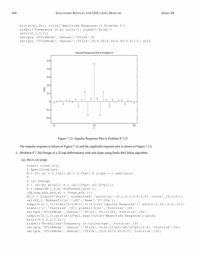
stem(n,h); title(’Impulse Response Plot in Problem 6’);axis([-1,M,min(h)-0.1,max(h)+0.1]); xlabel(’n’); ylabel(’h(n)’)set(gca,’XTickMode’,’manual’,’XTick’,[0;13;26],’fontsize’,12)%%% Amplitude Response PlotHf_2 = figure(’Units’,’normalized’,’position’,[0.1,0.1,0.8,0.8],’color’,[0,0,0]);set(Hf_2,’NumberTitle’,’off’,’Name’,’P7.21b’);
[Hr,w,a,L] = Hr_type1(h);
104 SOLUTIONS MANUAL FOR DSPUSING MATLAB APRIL 98
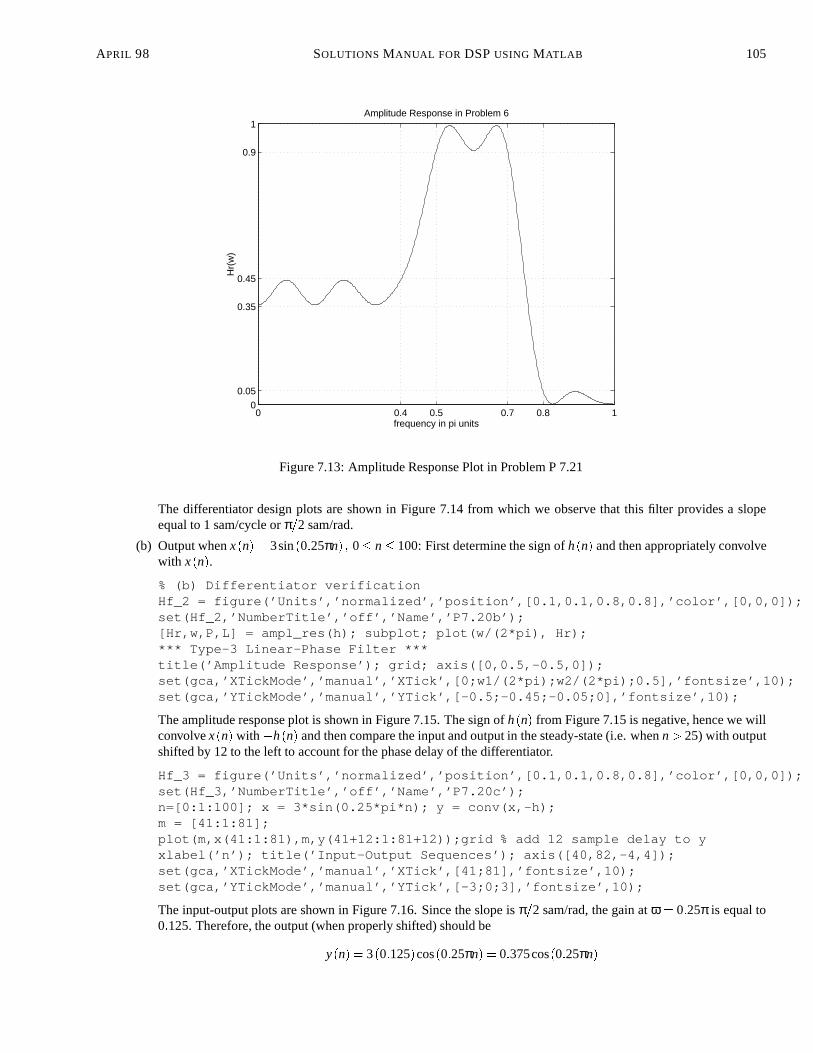
plot(w/pi,Hr); title(’Amplitude Response in Problem 6’)xlabel(’frequency in pi units’); ylabel(’Hr(w)’)axis([0,1,0,1])set(gca,’XTickMode’,’manual’,’XTick’,f)set(gca,’YTickMode’,’manual’,’YTick’,[0;0.05;0.35;0.45;0.9;1]); grid
0 13 26
−0.2
−0.1
0
0.1
0.2
0.3
0.4
0.5
n
h(n)
Impulse Response Plot in Problem 6
Figure 7.12: Impulse Response Plot in Problem P 7.21
The impulse response is shown in Figure 7.12 and the amplitude response plot is shown in Figure 7.13.
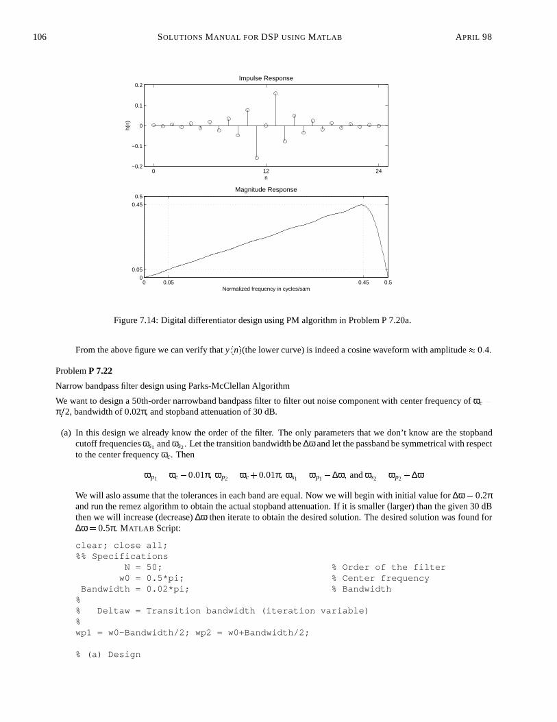
5. (Problem P 7.20) Design of a 25-tap differentiator with unit slope using Parks-McClellan algorithm
(a) MATLAB script:
clear; close all;% SpecificationsM = 25; w1 = 0.1*pi; w2 = 0.9*pi; % slope = 1 sam/cycle%% (a) Designf = [w1/pi w2/pi]; m = [w1/(2*pi) w2/(2*pi)];h = remez(M-1,f,m,’differentiator’);[db,mag,pha,grd,w] = freqz_m(h,1);Hf_1 = figure(’Units’,’normalized’,’position’,[0.1,0.1,0.8,0.8],’color’,[0,0,0]);set(Hf_1,’NumberTitle’,’off’,’Name’,’P7.20a’);subplot(2,1,1);stem([0:1:M-1],h);title(’Impulse Response’); axis([-1,25,-0.2,.2]);xlabel(’n’,’fontsize’,10); ylabel(’h(n)’,’fontsize’,10);set(gca,’XTickMode’,’manual’,’XTick’,[0;12;24],’fontsize’,10);subplot(2,1,2);plot(w/(2*pi),mag);title(’Magnitude Response’);grid;axis([0,0.5,0,0.5]);xlabel(’Normalized frequency in cycles/sam’,’fontsize’,10)set(gca,’XTickMode’,’manual’,’XTick’,[0;w1/(2*pi);w2/(2*pi);0.5],’fontsize’,10);set(gca,’YTickMode’,’manual’,’YTick’,[0;0.05;0.45;0.5],’fontsize’,10);
APRIL 98 SOLUTIONS MANUAL FOR DSPUSING MATLAB 105
0 0.4 0.5 0.7 0.8 10
0.05
0.35
0.45
0.9
1Amplitude Response in Problem 6
frequency in pi units
Hr(
w)
Figure 7.13: Amplitude Response Plot in Problem P 7.21
The differentiator design plots are shown in Figure 7.14 from which we observe that this filter provides a slopeequal to 1 sam/cycle orπ=2 sam/rad.
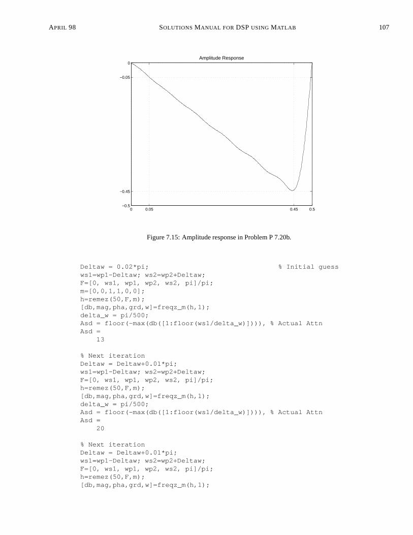
(b) Output whenx(n) = 3sin(0:25πn) ; 0� n� 100: First determine the sign ofh(n) and then appropriately convolvewith x(n).
% (b) Differentiator verificationHf_2 = figure(’Units’,’normalized’,’position’,[0.1,0.1,0.8,0.8],’color’,[0,0,0]);set(Hf_2,’NumberTitle’,’off’,’Name’,’P7.20b’);[Hr,w,P,L] = ampl_res(h); subplot; plot(w/(2*pi), Hr);*** Type-3 Linear-Phase Filter ***title(’Amplitude Response’); grid; axis([0,0.5,-0.5,0]);set(gca,’XTickMode’,’manual’,’XTick’,[0;w1/(2*pi);w2/(2*pi);0.5],’fontsize’,10);set(gca,’YTickMode’,’manual’,’YTick’,[-0.5;-0.45;-0.05;0],’fontsize’,10);
The amplitude response plot is shown in Figure 7.15. The sign ofh(n) from Figure 7.15 is negative, hence we willconvolvex(n) with �h(n) and then compare the input and output in the steady-state (i.e. whenn> 25) with outputshifted by 12 to the left to account for the phase delay of the differentiator.
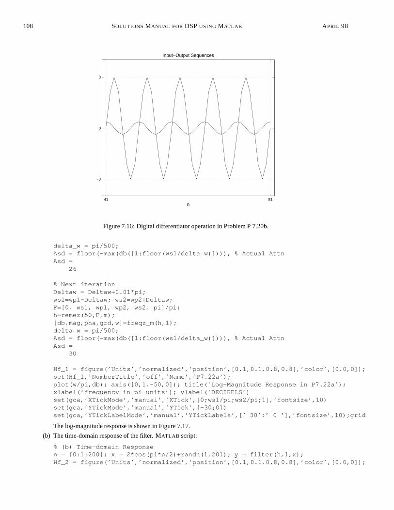
Hf_3 = figure(’Units’,’normalized’,’position’,[0.1,0.1,0.8,0.8],’color’,[0,0,0]);set(Hf_3,’NumberTitle’,’off’,’Name’,’P7.20c’);n=[0:1:100]; x = 3*sin(0.25*pi*n); y = conv(x,-h);m = [41:1:81];plot(m,x(41:1:81),m,y(41+12:1:81+12));grid % add 12 sample delay to yxlabel(’n’); title(’Input-Output Sequences’); axis([40,82,-4,4]);set(gca,’XTickMode’,’manual’,’XTick’,[41;81],’fontsize’,10);set(gca,’YTickMode’,’manual’,’YTick’,[-3;0;3],’fontsize’,10);
The input-output plots are shown in Figure 7.16. Since the slope isπ=2 sam/rad, the gain atω = 0:25π is equal to0:125. Therefore, the output (when properly shifted) should be
y(n) = 3(0:125)cos(0:25πn) = 0:375cos(0:25πn)
106 SOLUTIONS MANUAL FOR DSPUSING MATLAB APRIL 98
0 12 24−0.2
−0.1
0
0.1
0.2
n
h(n)
Impulse Response
0 0.05 0.45 0.50
0.05
0.45
0.5Magnitude Response
Normalized frequency in cycles/sam
Figure 7.14: Digital differentiator design using PM algorithm in Problem P 7.20a.
From the above figure we can verify thaty(n)(the lower curve) is indeed a cosine waveform with amplitude� 0:4.
ProblemP 7.22
Narrow bandpass filter design using Parks-McClellan Algorithm
We want to design a 50th-order narrowband bandpass filter to filter out noise component with center frequency ofωc =π=2, bandwidth of 0:02π, and stopband attenuation of 30 dB.
(a) In this design we already know the order of the filter. The only parameters that we don’t know are the stopbandcutoff frequenciesωs1 andωs2. Let the transition bandwidth be∆ω and let the passband be symmetrical with respectto the center frequencyωc. Then
ωp1 = ωc�0:01π; ωp2 = ωc+0:01π; ωs1 = ωp1�∆ω; andωs2 = ωp2 +∆ω
We will aslo assume that the tolerances in each band are equal. Now we will begin with initial value for∆ω = 0:2πand run the remez algorithm to obtain the actual stopband attenuation. If it is smaller (larger) than the given 30 dBthen we will increase (decrease)∆ω then iterate to obtain the desired solution. The desired solution was found for∆ω = 0:5π. MATLAB Script:
clear; close all;%% Specifications
N = 50; % Order of the filterw0 = 0.5*pi; % Center frequency
Bandwidth = 0.02*pi; % Bandwidth%% Deltaw = Transition bandwidth (iteration variable)%wp1 = w0-Bandwidth/2; wp2 = w0+Bandwidth/2;
% (a) Design
APRIL 98 SOLUTIONS MANUAL FOR DSPUSING MATLAB 107
0 0.05 0.45 0.5−0.5
−0.45
−0.05
0Amplitude Response
Figure 7.15: Amplitude response in Problem P 7.20b.
Deltaw = 0.02*pi; % Initial guessws1=wp1-Deltaw; ws2=wp2+Deltaw;F=[0, ws1, wp1, wp2, ws2, pi]/pi;m=[0,0,1,1,0,0];h=remez(50,F,m);[db,mag,pha,grd,w]=freqz_m(h,1);delta_w = pi/500;Asd = floor(-max(db([1:floor(ws1/delta_w)]))), % Actual AttnAsd =
13
% Next iterationDeltaw = Deltaw+0.01*pi;ws1=wp1-Deltaw; ws2=wp2+Deltaw;F=[0, ws1, wp1, wp2, ws2, pi]/pi;h=remez(50,F,m);[db,mag,pha,grd,w]=freqz_m(h,1);delta_w = pi/500;Asd = floor(-max(db([1:floor(ws1/delta_w)]))), % Actual AttnAsd =
20
% Next iterationDeltaw = Deltaw+0.01*pi;ws1=wp1-Deltaw; ws2=wp2+Deltaw;F=[0, ws1, wp1, wp2, ws2, pi]/pi;h=remez(50,F,m);[db,mag,pha,grd,w]=freqz_m(h,1);
108 SOLUTIONS MANUAL FOR DSPUSING MATLAB APRIL 98
41 81
−3
0
3
n
Input−Output Sequences
Figure 7.16: Digital differentiator operation in Problem P 7.20b.
delta_w = pi/500;Asd = floor(-max(db([1:floor(ws1/delta_w)]))), % Actual AttnAsd =
26
% Next iterationDeltaw = Deltaw+0.01*pi;ws1=wp1-Deltaw; ws2=wp2+Deltaw;F=[0, ws1, wp1, wp2, ws2, pi]/pi;h=remez(50,F,m);[db,mag,pha,grd,w]=freqz_m(h,1);delta_w = pi/500;Asd = floor(-max(db([1:floor(ws1/delta_w)]))), % Actual AttnAsd =
30
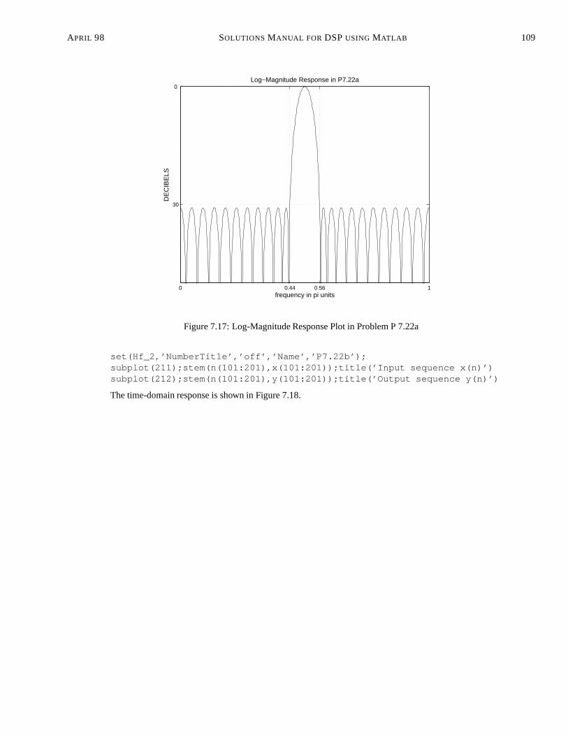
Hf_1 = figure(’Units’,’normalized’,’position’,[0.1,0.1,0.8,0.8],’color’,[0,0,0]);set(Hf_1,’NumberTitle’,’off’,’Name’,’P7.22a’);plot(w/pi,db); axis([0,1,-50,0]); title(’Log-Magnitude Response in P7.22a’);xlabel(’frequency in pi units’); ylabel(’DECIBELS’)set(gca,’XTickMode’,’manual’,’XTick’,[0;ws1/pi;ws2/pi;1],’fontsize’,10)set(gca,’YTickMode’,’manual’,’YTick’,[-30;0])set(gca,’YTickLabelMode’,’manual’,’YTickLabels’,[’ 30’;’ 0 ’],’fontsize’,10);grid
The log-magnitude response is shown in Figure 7.17.
(b) The time-domain response of the filter. MATLAB script:
% (b) Time-domain Responsen = [0:1:200]; x = 2*cos(pi*n/2)+randn(1,201); y = filter(h,1,x);Hf_2 = figure(’Units’,’normalized’,’position’,[0.1,0.1,0.8,0.8],’color’,[0,0,0]);
APRIL 98 SOLUTIONS MANUAL FOR DSPUSING MATLAB 109
0 0.44 0.56 1
30
0 Log−Magnitude Response in P7.22a
frequency in pi units
DE
CIB
ELS
Figure 7.17: Log-Magnitude Response Plot in Problem P 7.22a
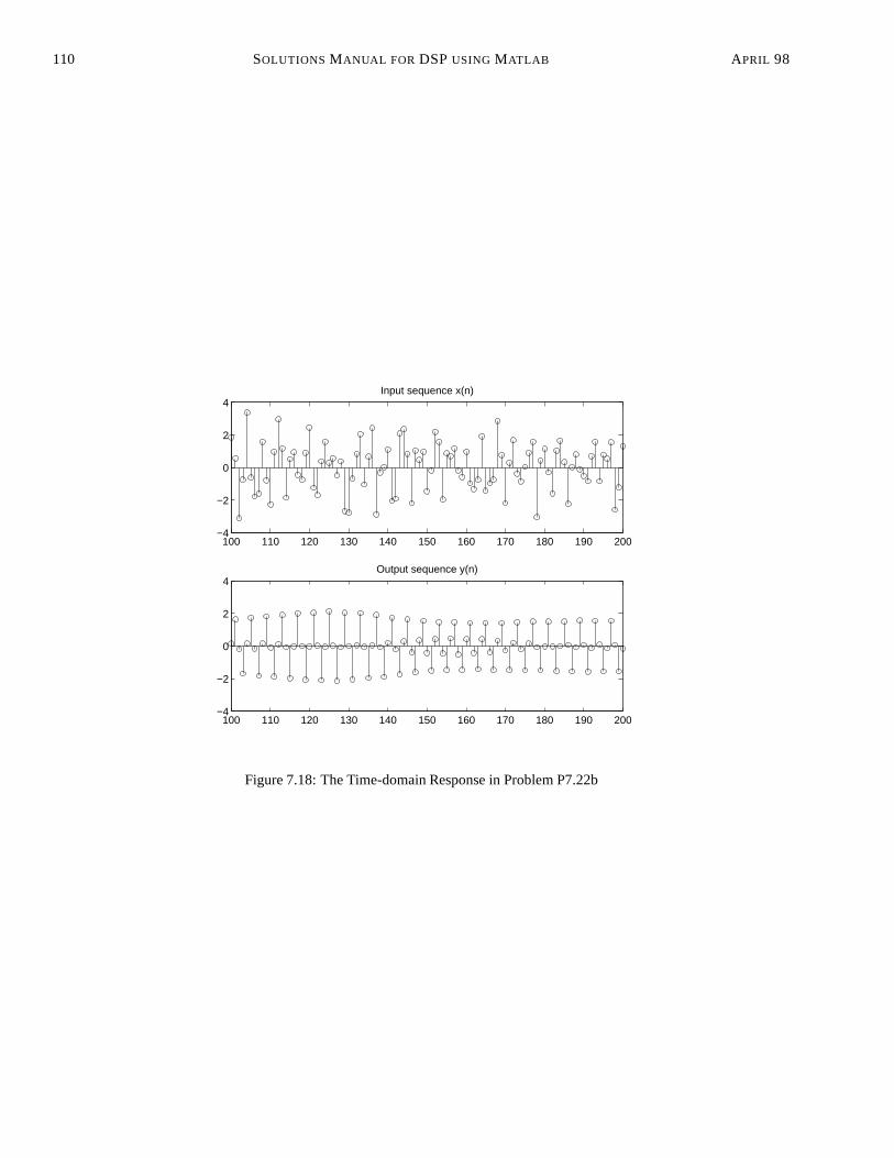
set(Hf_2,’NumberTitle’,’off’,’Name’,’P7.22b’);subplot(211);stem(n(101:201),x(101:201));title(’Input sequence x(n)’)subplot(212);stem(n(101:201),y(101:201));title(’Output sequence y(n)’)
The time-domain response is shown in Figure 7.18.
110 SOLUTIONS MANUAL FOR DSPUSING MATLAB APRIL 98
100 110 120 130 140 150 160 170 180 190 200−4
−2
0
2
4Input sequence x(n)
100 110 120 130 140 150 160 170 180 190 200−4
−2
0
2
4Output sequence y(n)
Figure 7.18: The Time-domain Response in Problem P7.22b