Some concepts from Dark Energy and Statistical methods

Dragan Huterer

Physics DepartmentUniversity of Michigan

Some concepts fromDark Energy

and Statistical methods

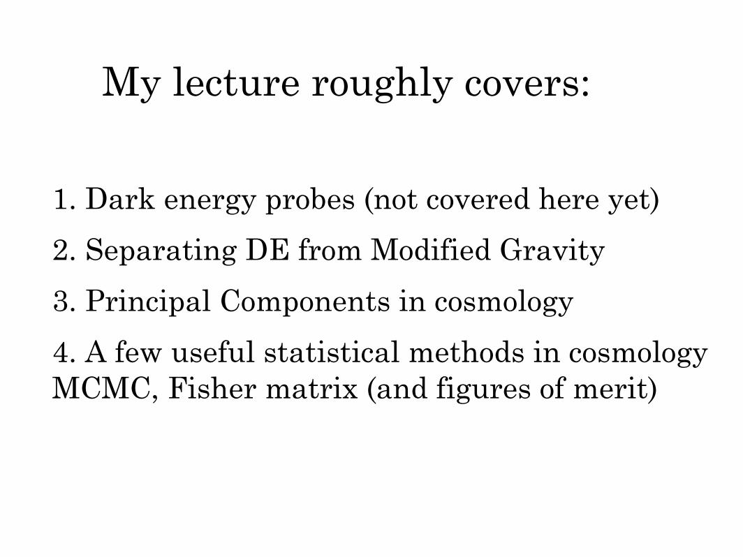
1. Dark energy probes (not covered here yet)

2. Separating DE from Modified Gravity

3. Principal Components in cosmology

4. A few useful statistical methods in cosmology MCMC, Fisher matrix (and figures of merit)

My lecture roughly covers:

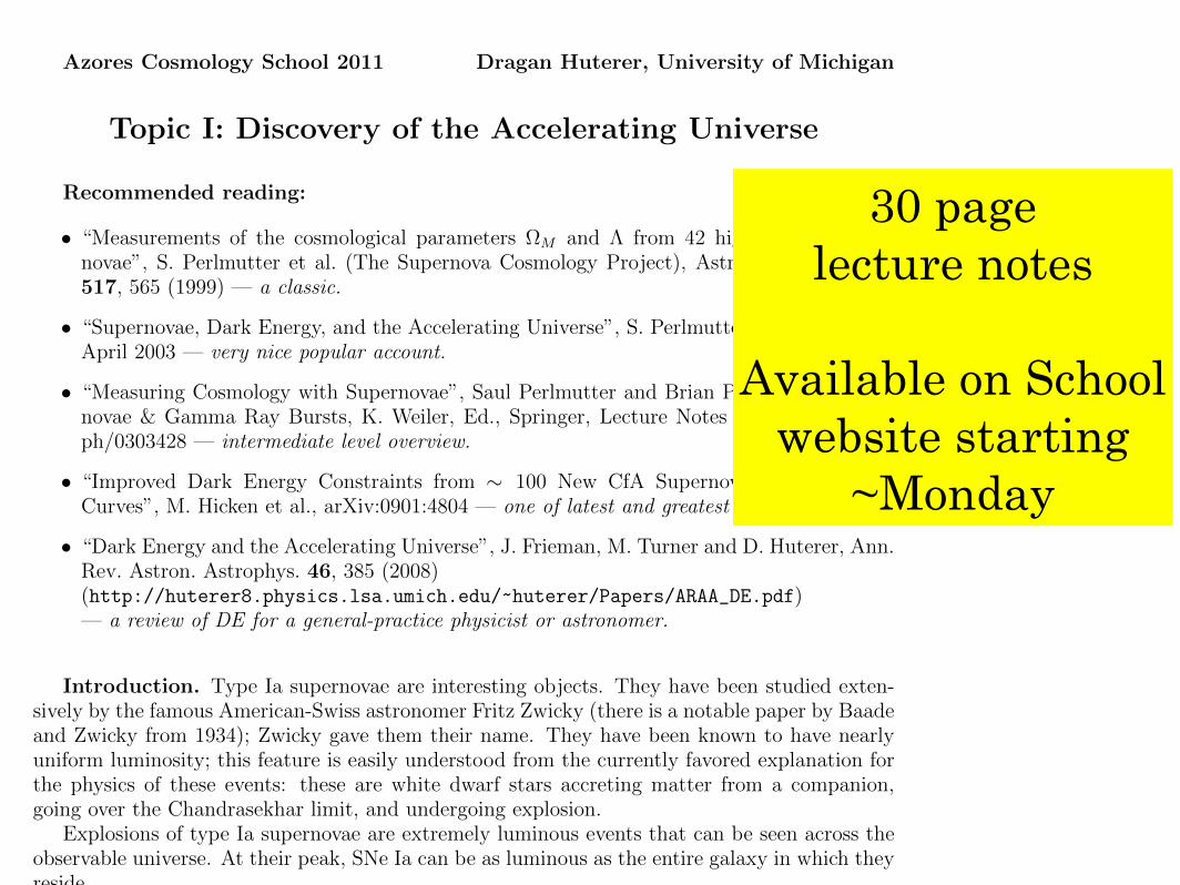
Azores Cosmology School 2011 Dragan Huterer, University of Michigan

Topic I: Discovery of the Accelerating Universe

Recommended reading:

• “Measurements of the cosmological parameters ΩM and Λ from 42 high-redshift super-

novae”, S. Perlmutter et al. (The Supernova Cosmology Project), Astrophysical Journal

517, 565 (1999) — a classic.

• “Supernovae, Dark Energy, and the Accelerating Universe”, S. Perlmutter, Physics Today,

April 2003 — very nice popular account.

• “Measuring Cosmology with Supernovae”, Saul Perlmutter and Brian P. Schmidt, Super-

novae & Gamma Ray Bursts, K. Weiler, Ed., Springer, Lecture Notes in Physics, astro-

ph/0303428 — intermediate level overview.

• “Improved Dark Energy Constraints from ∼ 100 New CfA Supernova Type Ia Light

Curves”, M. Hicken et al., arXiv:0901:4804 — one of latest and greatest SN Ia data sets.

• “Dark Energy and the Accelerating Universe”, J. Frieman, M. Turner and D. Huterer, Ann.

Rev. Astron. Astrophys. 46, 385 (2008)

(http://huterer8.physics.lsa.umich.edu/~huterer/Papers/ARAA_DE.pdf)— a review of DE for a general-practice physicist or astronomer.

Introduction. Type Ia supernovae are interesting objects. They have been studied exten-

sively by the famous American-Swiss astronomer Fritz Zwicky (there is a notable paper by Baade

and Zwicky from 1934); Zwicky gave them their name. They have been known to have nearly

uniform luminosity; this feature is easily understood from the currently favored explanation for

the physics of these events: these are white dwarf stars accreting matter from a companion,

going over the Chandrasekhar limit, and undergoing explosion.

Explosions of type Ia supernovae are extremely luminous events that can be seen across the

observable universe. At their peak, SNe Ia can be as luminous as the entire galaxy in which they

reside.

Standard candles. It is very difficult to measure distances in astronomy. You can get red-

shift of an object from its spectrum, but how do you get the distance? There are many empirical

— and uncertain — ways to do so (surface brightness fluctuations, period-luminosity relation of

Cepheids, proper motions, etc). Typically, astronomers construct an unwieldy “distance ladder”

to measure distance to a distant galaxy: they use some of these relations (say, proper motions)

to calibrate distances to more nearby objects, then go from those objects to more distant ones

using other relations that work better in that distance regime. This procedure is clearly not

robust.

A “standard candle” is a hypothetical object that has a fixed luminosity (that is, fixed intrinsic

power that it radiates). Having a standard candle would be useful since then you could infer

distances from objects just by using the inverse square law, f = L/(4πd2), by measuring the flux

f and knowing the luminosity L from the standard candle property. In fact, you don’t even to

know the luminosity of the standard candle to be able to infer relative distances to objects – all

you need to know that thus luminosity is the same for all objects.

1

30 page lecture notes

Available on School website starting

~Monday

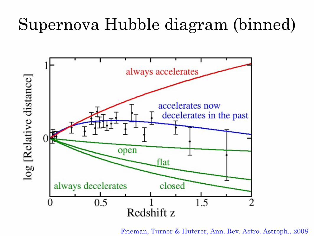
Supernova Hubble diagram (binned)

Frieman, Turner & Huterer, Ann. Rev. Astro. Astroph., 2008

Bruce

Alex

Alessandro

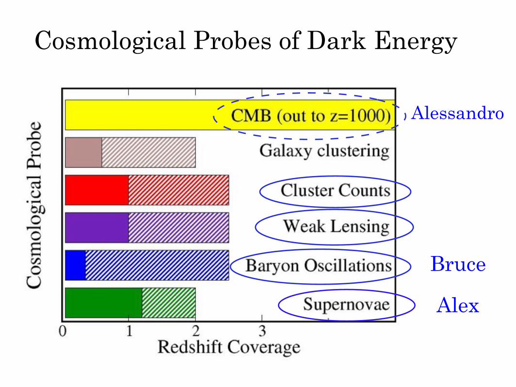
Cosmological Probes of Dark Energy

Supernova Hubble diagram (binned)


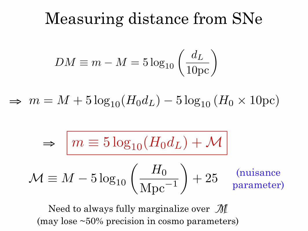
Measuring distance from SNe

DM ≡ m−M = 5 log10

dL

10pc

m = M + 5 log10(H0dL)− 5 log10 (H0 × 10pc)

m ≡ 5 log10(H0dL) +M

M ≡M − 5 log10

H0

Mpc−1

+ 25

⇒

⇒

Need to always fully marginalize over M (may lose ~50% precision in cosmo parameters)

(nuisanceparameter)

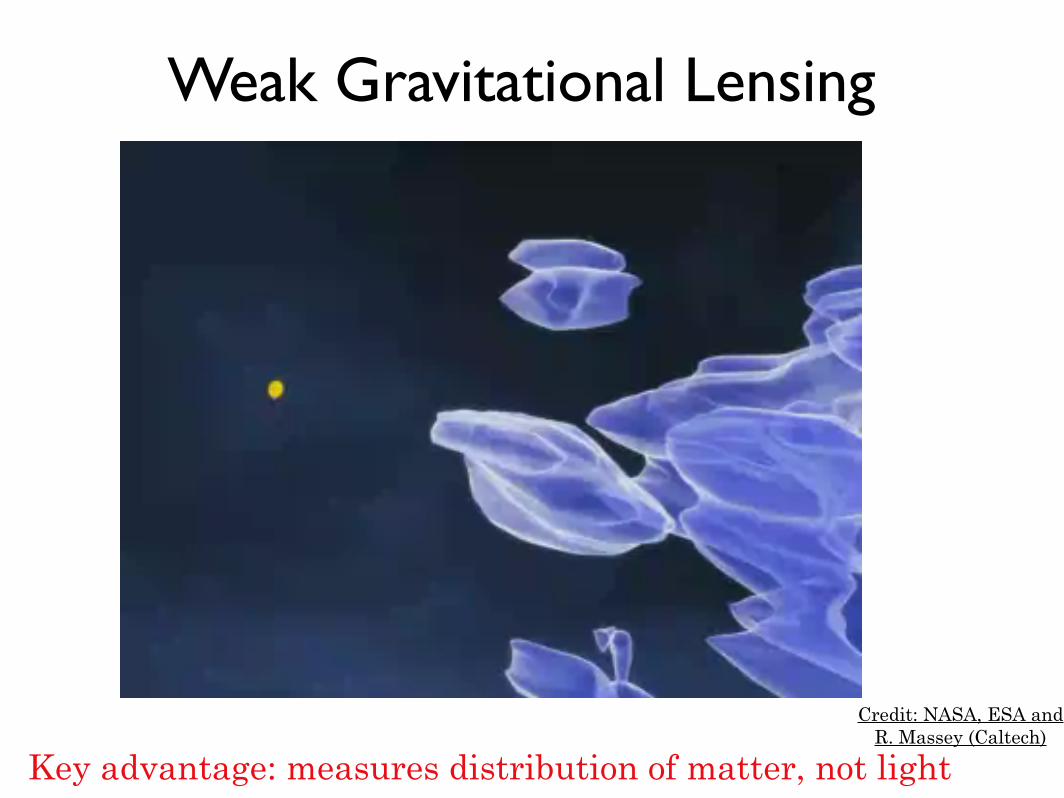
Weak Gravitational Lensing

Key advantage: measures distribution of matter, not light

Credit: NASA, ESA and R. Massey (Caltech)

http://www.lsst.org

http://www.lsst.org

http://www.lsst.org

http://www.lsst.org

Weak Gravitational Lensing

Credit: Colombi & Mellier

http://www.lsst.org

http://www.lsst.org

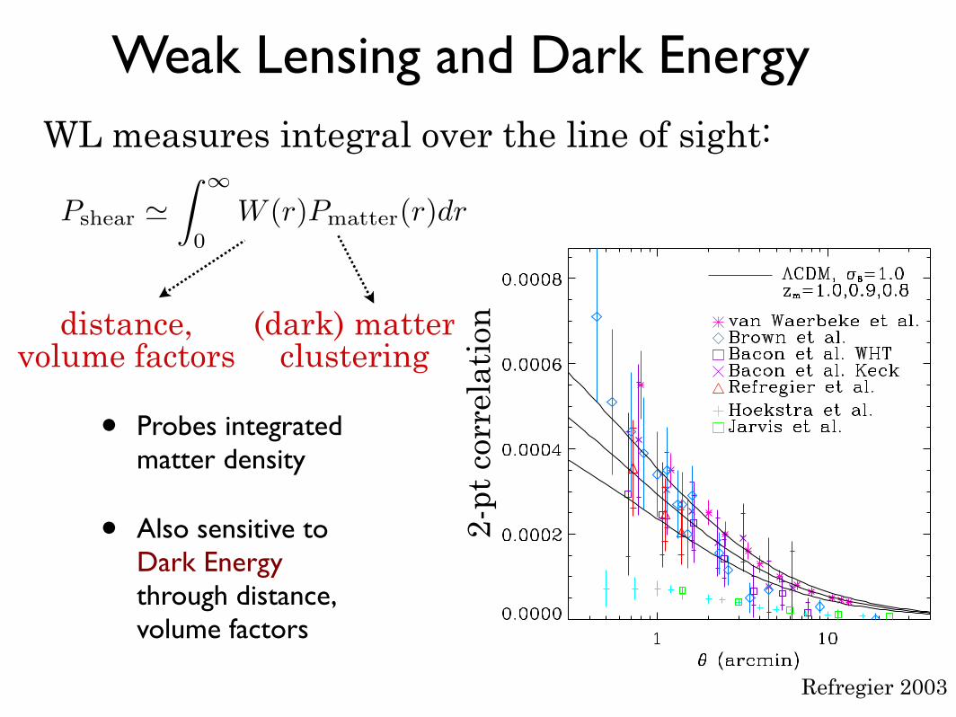
Weak Lensing and Dark Energy

• Probes integrated matter density

• Also sensitive to Dark Energy through distance, volume factors

Refregier 2003

distance,volume factors

(dark) matterclustering

2-pt

cor

rela

tion

WL measures integral over the line of sight:

Pshear !

∫∞

0

W (r)Pmatter(r)dr

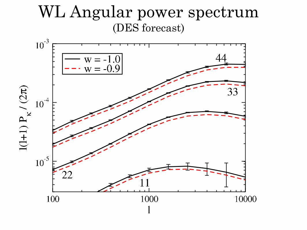
WL Angular power spectrum(DES forecast)

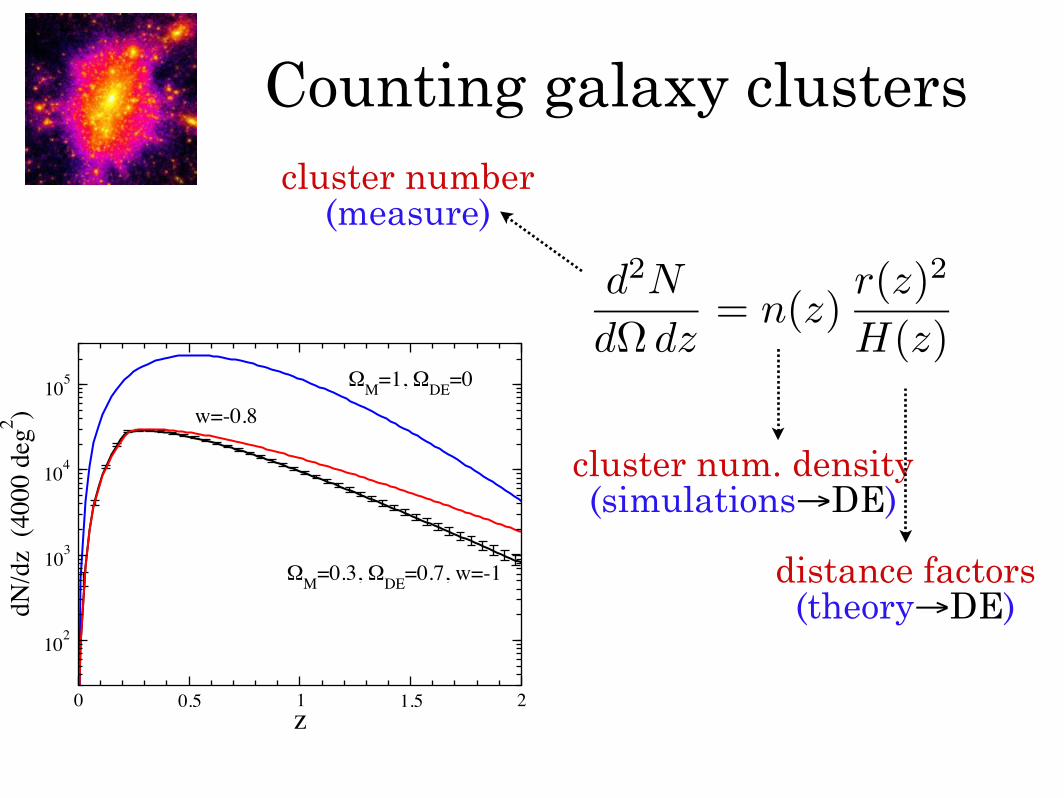
Counting galaxy clusters

d2N

dΩ dz= n(z)

r(z)2

H(z)

0 0.5 1 1.5 2z

102

103

104

105

dN/d

z (4

000

deg2 )

ΩM=1, ΩDE=0

ΩM=0.3, ΩDE=0.7, w=-1

w=-0.8

cluster number(measure)

cluster num. density(simulations→DE)

distance factors(theory→DE)

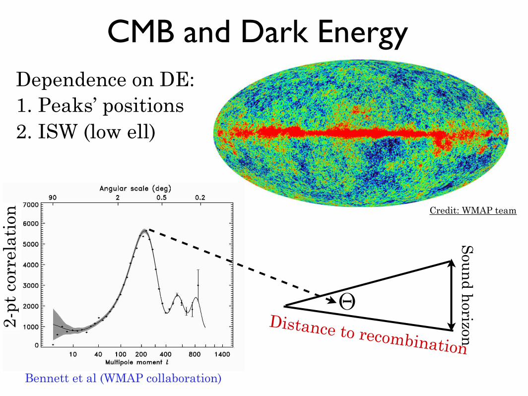
CMB and Dark EnergyS

oun

d horizon

Distance to recombination

Bennett et al (WMAP collaboration)

Credit: WMAP team

Θ

2-pt

cor

rela

tion

Dependence on DE:1. Peaks’ positions2. ISW (low ell)

http://www.lsst.org

http://www.lsst.org

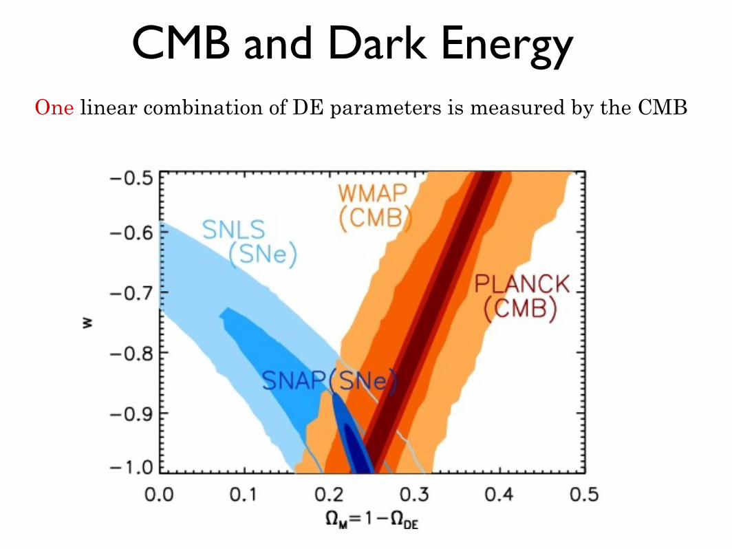
CMB and Dark EnergyOne linear combination of DE parameters is measured by the CMB

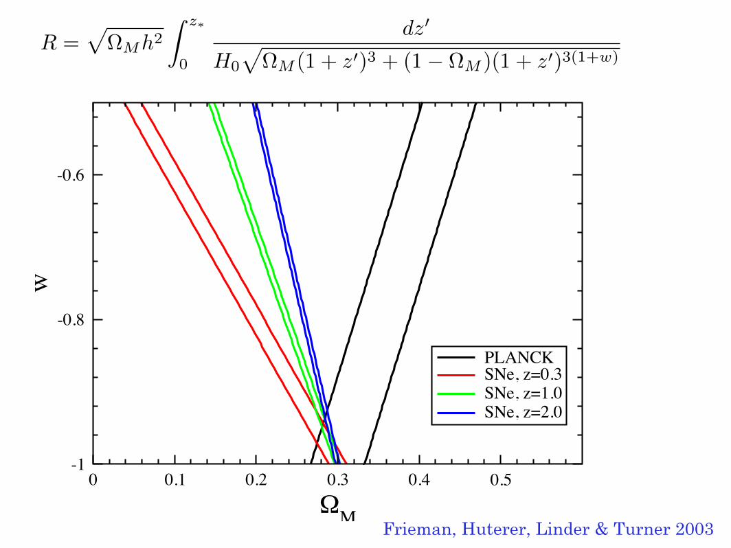
0 0.1 0.2 0.3 0.4 0.5!M

-1

-0.8

-0.6

w

PLANCKSNe, z=0.3SNe, z=1.0SNe, z=2.0

Frieman, Huterer, Linder & Turner 2003

R =ΩMh2

z∗

0

dz

H0

ΩM (1 + z)3 + (1− ΩM )(1 + z)3(1+w)

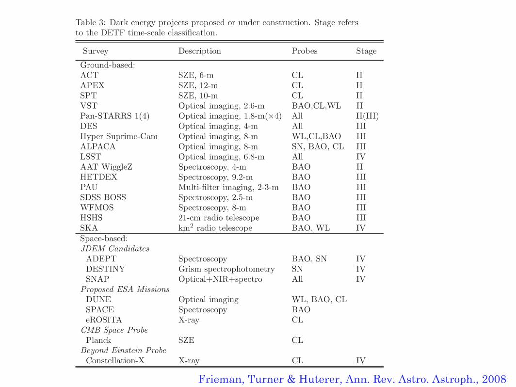
40 Frieman, Turner & Huterer

Table 3: Dark energy projects proposed or under construction. Stage refersto the DETF time-scale classification.

Survey Description Probes Stage

Ground-based:ACT SZE, 6-m CL IIAPEX SZE, 12-m CL IISPT SZE, 10-m CL IIVST Optical imaging, 2.6-m BAO,CL,WL IIPan-STARRS 1(4) Optical imaging, 1.8-m(×4) All II(III)DES Optical imaging, 4-m All IIIHyper Suprime-Cam Optical imaging, 8-m WL,CL,BAO IIIALPACA Optical imaging, 8-m SN, BAO, CL IIILSST Optical imaging, 6.8-m All IVAAT WiggleZ Spectroscopy, 4-m BAO IIHETDEX Spectroscopy, 9.2-m BAO IIIPAU Multi-filter imaging, 2-3-m BAO IIISDSS BOSS Spectroscopy, 2.5-m BAO IIIWFMOS Spectroscopy, 8-m BAO IIIHSHS 21-cm radio telescope BAO IIISKA km2 radio telescope BAO, WL IVSpace-based:JDEM Candidates

ADEPT Spectroscopy BAO, SN IVDESTINY Grism spectrophotometry SN IVSNAP Optical+NIR+spectro All IV

Proposed ESA MissionsDUNE Optical imaging WL, BAO, CLSPACE Spectroscopy BAOeROSITA X-ray CL

CMB Space ProbePlanck SZE CL

Beyond Einstein ProbeConstellation-X X-ray CL IV

8.2 Space-based surveys

Three of the proposed space projects are candidates for the Joint Dark EnergyMission (JDEM), a joint mission of the U.S. Department of Energy (DOE) andthe NASA Beyond Einstein program, targeted at dark energy science. Super-Nova/Acceleration Probe (SNAP) proposes to study dark energy using a dedi-cated 2-m class telescope. With imaging in 9 optical and near-infrared passbandsand follow-up spectroscopy of supernovae, it is principally designed to probe SNeIa and weak lensing, taking advantage of the excellent optical image quality andnear-infrared transparency of a space-based platform. Fig. 17 gives an illustra-tion of the statistical constraints that the proposed SNAP mission could achieve,by combining SN and weak lensing observations with results from the PlanckCMB mission. This forecast makes use of the Fisher information matrix de-


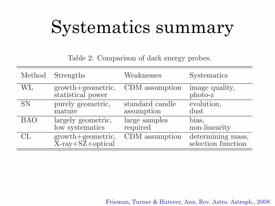
Systematics summary38 Frieman, Turner & Huterer

Table 2: Comparison of dark energy probes.

Method Strengths Weaknesses Systematics

WL growth+geometric, CDM assumption image quality,statistical power photo-z

SN purely geometric, standard candle evolution,mature assumption dust

BAO largely geometric, large samples bias,low systematics required non-linearity

CL growth+geometric, CDM assumption determining mass,X-ray+SZ+optical selection function

8 DARK ENERGY PROJECTS

A diverse and ambitious set of projects to probe dark energy are in progress orbeing planned. Here we provide a brief overview of the observational landscape.With the exception of experiments at the LHC that might shed light on darkenergy through discoveries about supersymmetry or dark matter, all plannedexperiments involve cosmological observations. Table 3 provides a representativesampling, not a comprehensive listing, of projects that are currently proposed orunder construction and does not include experiments that have already reportedresults. All of these projects share the common feature of surveying wide areasto collect large samples of objects — galaxies, clusters, or supernovae.

The Dark Energy Task Force (DETF) report (Albrecht et al. 2006) classifieddark energy surveys into an approximate sequence: on-going projects, eithertaking data or soon to be taking data, are Stage II; near-future, intermediate-scaleprojects are Stage III; and larger-scale, longer-term future projects are designatedStage IV. More advanced stages are in general expected to deliver tighter darkenergy constraints, which the DETF quantified using the w0-wa figure of merit(FoM) discussed in the Appendix (§11.1). Stage III experiments are expectedto deliver a factor ∼ 3 − 5 improvement in the DETF FoM compared to thecombined Stage II results, while Stage IV experiments should improve the FoMby roughly a factor of 10 compared to Stage II, though these estimates are onlyindicative and are subject to considerable uncertainties in systematic errors (seeFig. 16).

We divide our discussion into ground- and space-based surveys. Ground-basedprojects are typically less expensive than their space-based counterparts and canemploy larger-aperture telescopes. The discovery of dark energy and many of thesubsequent observations to date have been dominated by ground-based telescopes.On the other hand, HST (high-redshift SN observations), Chandra (X-ray clus-ters), and WMAP CMB observations have played critical roles in probing darkenergy. While more challenging to execute, space-based surveys offer the advan-tages of observations unhindered by weather and by the scattering, absorption,and emission by the atmosphere, stable observing platforms free of time-changinggravitational loading, and the ability to continuously observe away from the sunand moon. They therefore have the potential for much improved control of sys-tematic errors.


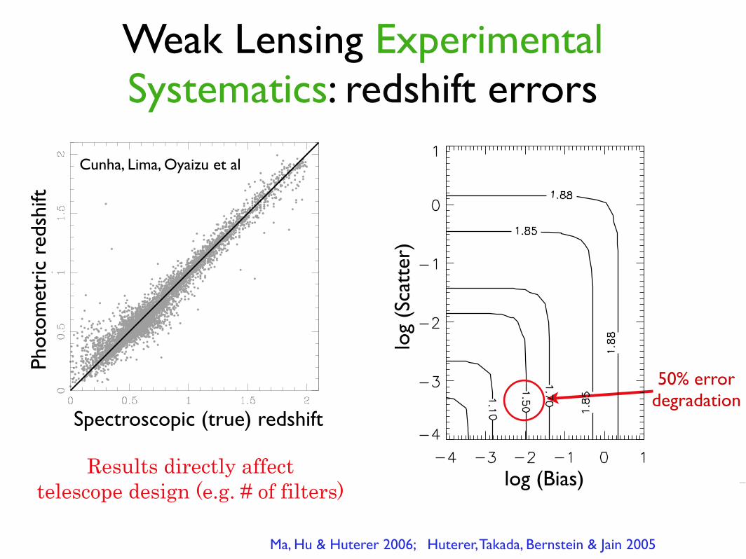
Weak Lensing Experimental Systematics: redshift errors

Ma, Hu & Huterer 2006; Huterer, Takada, Bernstein & Jain 2005

Spectroscopic (true) redshift

Phot

omet

ric

reds

hift

Cunha, Lima, Oyaizu et al

log (Bias)

log

(Sca

tter

)50% error

degradation

Results directly affect telescope design (e.g. # of filters)

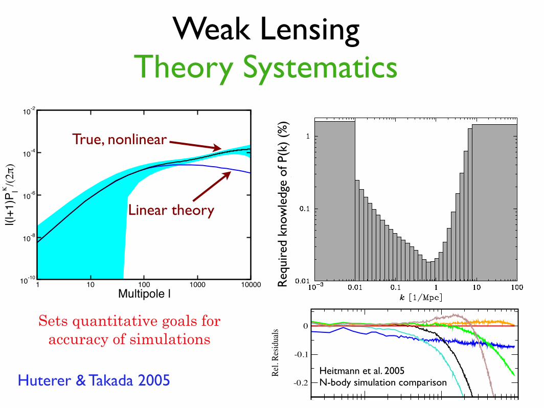
Weak LensingTheory Systematics

1 10 100 1000 10000Multipole l

10-10

10-8

10-6

10-4

10-2

l(l+1

)Plκ/(2π)

Huterer & Takada 2005

True, nonlinear

Linear theory

-0.2

-0.1

0

Rel.

Resid

uals

0.1 1 10k[Mpc-1]

10

100

1000

10000

P(k)

[Mpc

3 ]

MC2 (Richardson)MC2 (10243)FLASHHOTGADGETHYDRATPM

Heitmann et al. 2005 N-body simulation comparison

Req

uire

d kn

owle

dge

of P

(k)

(%)

Sets quantitative goals foraccuracy of simulations

What if gravity deviates from GR?

H2− F (H) =

8πG

3ρ, or H2 =

8πG

3

(

ρ +3F (H)

8πG

)

For example:

Modified gravity Dark energy

ρDE(z) = ρDE,0 exp

3 z

0(1 + w(z))d ln(1 + z)

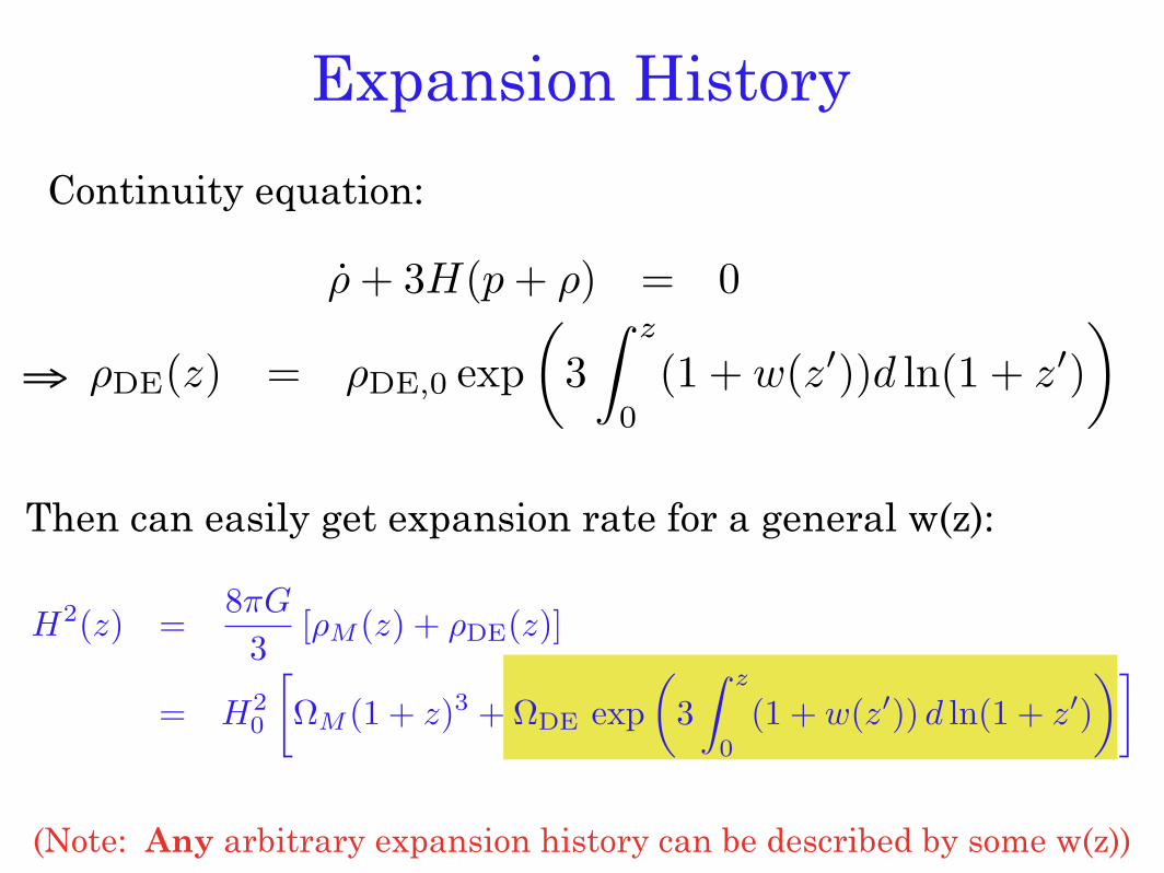
ρ + 3H(p + ρ) = 0

Expansion History

Continuity equation:

Then can easily get expansion rate for a general w(z):

H2(z) =

8πG

3[ρM (z) + ρDE(z)]

= H20

ΩM (1 + z)3 + ΩDE exp

3

z

0(1 + w(z)) d ln(1 + z

)

(Note: Any arbitrary expansion history can be described by some w(z))

⇒

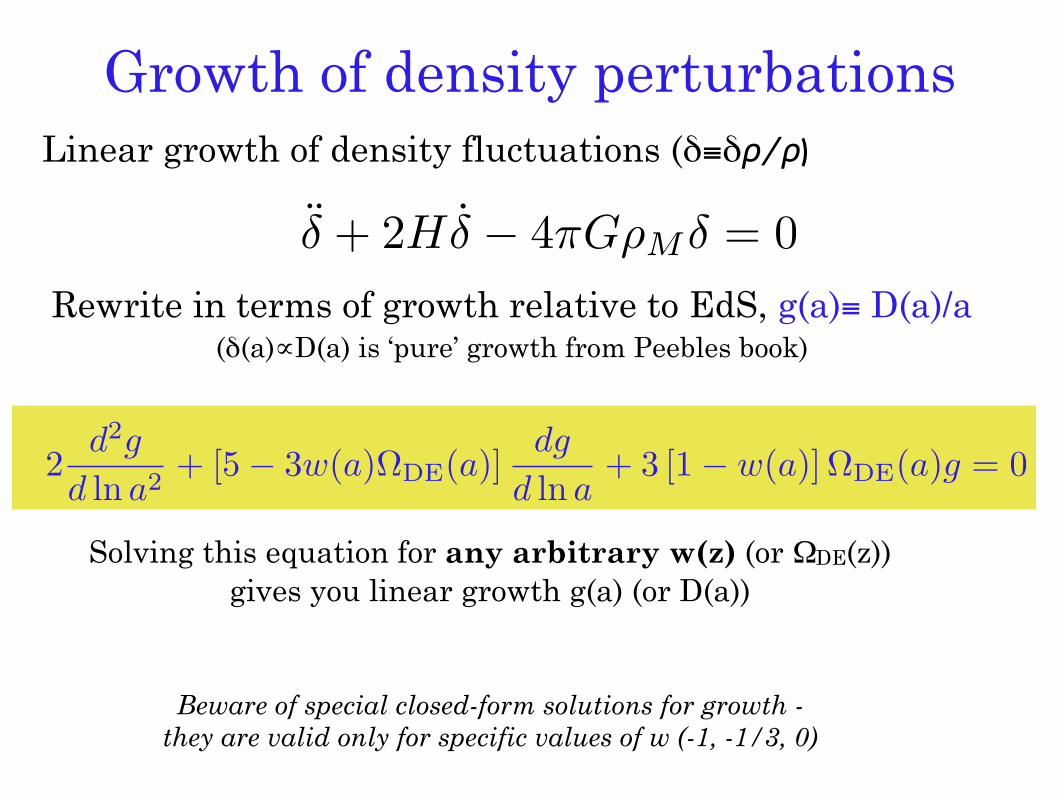
Growth of density perturbationsLinear growth of density fluctuations (δ≡δρ/ρ)

δ + 2H δ − 4πGρMδ = 0Rewrite in terms of growth relative to EdS, g(a)≡ D(a)/a

(δ(a)∝D(a) is ‘pure’ growth from Peebles book)

2d2g

d ln a2+ [5− 3w(a)ΩDE(a)]

dg

d ln a+ 3 [1− w(a)] ΩDE(a)g = 0

Solving this equation for any arbitrary w(z) (or ΩDE(z))gives you linear growth g(a) (or D(a))

Beware of special closed-form solutions for growth - they are valid only for specific values of w (-1, -1/3, 0)

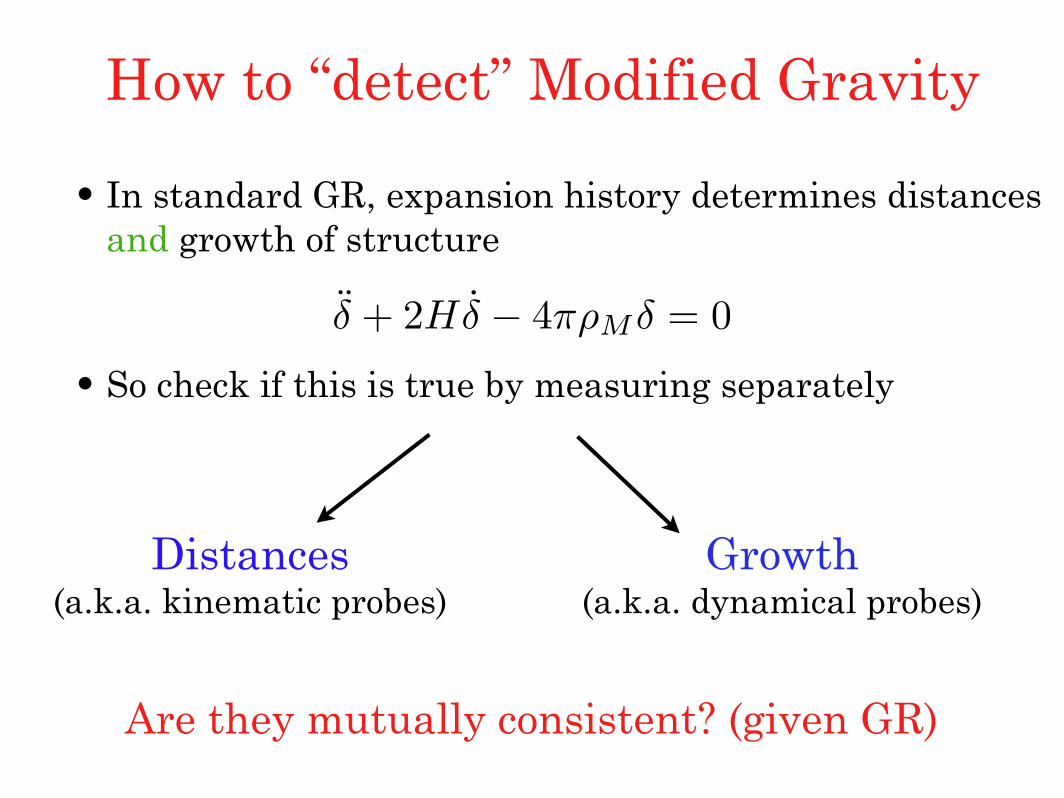
•In standard GR, expansion history determines distances and growth of structure

•So check if this is true by measuring separately

δ + 2H δ − 4πρMδ = 0

Distances(a.k.a. kinematic probes)

Growth(a.k.a. dynamical probes)

How to “detect” Modified Gravity

Are they mutually consistent? (given GR)

Principal Components:asking the data what it measures

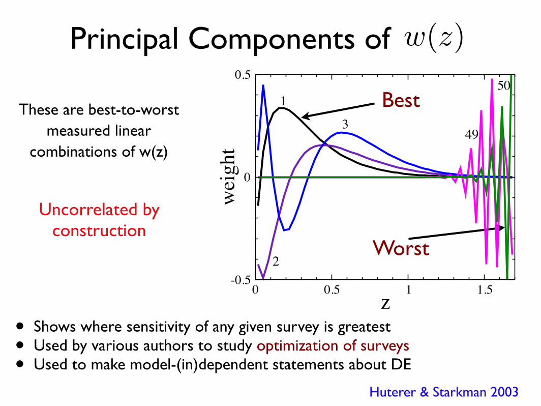
Principal Components of w(z)

Huterer & Starkman 2003

• Shows where sensitivity of any given survey is greatest• Used by various authors to study optimization of surveys• Used to make model-(in)dependent statements about DE

Worst

BestThese are best-to-worstmeasured linear

combinations of w(z)

0 0.5 1 1.5z

-0.5

0

0.5

wei

ght

1

2

349

50

Uncorrelated by construction

0 0.2 0.4 0.6 0.8 1 1.2z-2

-1

0

1

2

3

e i(z)

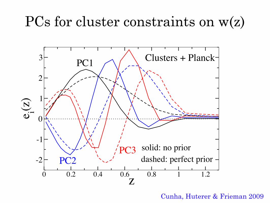
solid: no priordashed: perfect priorPC2

PC3

PC1 Clusters + Planck

PCs for cluster constraints on w(z)

Cunha, Huterer & Frieman 2009

3

z10 15

(a) Best

(b) Worst

20 25

!x!x

-0.5

0

0.5

-0.5

0

0.5

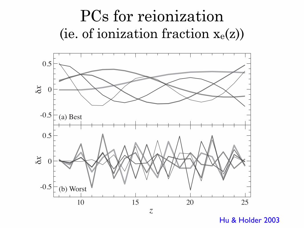
FIG. 3: Eigenmodes. (a) 5 best (decreasing eigenvalue thickto thin) constrained eigenmodes or linear combinations of ion-ization history. (b) 5 worst constrained eigenmodes.

of fiducial model, the linear response approximation canprovide useful tools for representing the data. A detailedconsideration is beyond the scope of this work. Insteadwe will show that a modification of the forward approachsuffices to extract essentially all of the information in theCMB.

III. CMB OBSERVABLES

To better quantify the information contained in thepower spectrum, let us consider the ultimate limit of anall-sky experiment that is cosmic variance limited. Thevariance of the power spectrum is then given by

⟨

δCEE! δCEE

!′⟩

=2

2" + 1(CEE

l )2δ!!′ (3)

and hence the covariance of the ionization parameters〈δx(zi)δx(zj)〉 ≈ (F−1)ij , where

Fij =∑

!

(" + 1/2)T!iT!j (4)

is the Fisher matrix. The structure of the transfer matriximplies a large covariance between estimates of δx(zi)and renders the delta-function representation difficult tovisualize.

Consider instead the principal component representa-tion based on the orthonormal eigenvectors of the Fishermatrix, decomposed as

Fij =∑

µ

Siµσ−2µ Sjµ . (5)

For a fixed µ, the Siµ specify linear combinations of theδx(zi) for a new representation of the data

mµ =∑

i

Siµδxi , (6)

mode µ5 10 15

"µ

#µ

"# (cumul.)

prior

prior

10-5

10-4

10-3

10-2

10-1

1

101

102

FIG. 4: Eigenmode statistics. Top curve: rms error σµ onmode amplitude; dashed line represents a physicality prior onx; only the first 5 modes contain interesting information. Bot-tom curve: optical depth per unit-amplitude mode τµ. Middlecurve: rms error on total optical depth shown as the cumula-tive contribution from modes ≤ µ; dashed line represents thephysicality prior on x.

where the covariance matrix of the mode amplitudes isgiven by

〈mµmν〉 = σ2µδµν . (7)

In other words, the eigenvectors form a new basis thatis complete and yields uncorrelated measurements withvariance given by the inverse eigenvalue. The largesteigenvalues correspond to the minimum variance direc-tions and the first 5 are shown in the upper panel ofFig. 3. The first two correspond essentially to the aver-age ionization at high redshift and low redshift respec-tively. The lower panel shows the directions with the 5highest variances. Here neighboring delta modes withsimilar responses compensate each other to leave the ob-servable power spectrum unchanged. The rms of eachmode is shown in Fig. 4. Because the ionization fractioncannot be negative and the amplitude of each mode is∼ 0.5, only the first 5 modes with σµ ! 1 have useful in-formation. An added benefit of the principal componentrepresentation is that the structure in the lowest modesis invariant under refinement of the binning scheme ∆z.In " space, the first mode controls the high " power, thesecond the low " power and the third through fifth adjustthe ringing in the spectrum.

These eigenmodes provide a good meeting ground be-tween observations and models. The amplitude mµ ofthese 5 best modes may be added to the usual CMB pa-rameter estimation chain and the results compared tomodel predictions for mµ without significant loss of in-formation. As an example, in Figure 5 we have repre-sented a complex ionization history (inset, thick-dashed)through its first 1 through 5 eigenmodes. For this ioniza-tion history the first 3 eigenmodes suffice to recover theobservable power spectrum. The temperature polariza-

Hu & Holder 2003

PCs for reionization (ie. of ionization fraction xe(z))

2

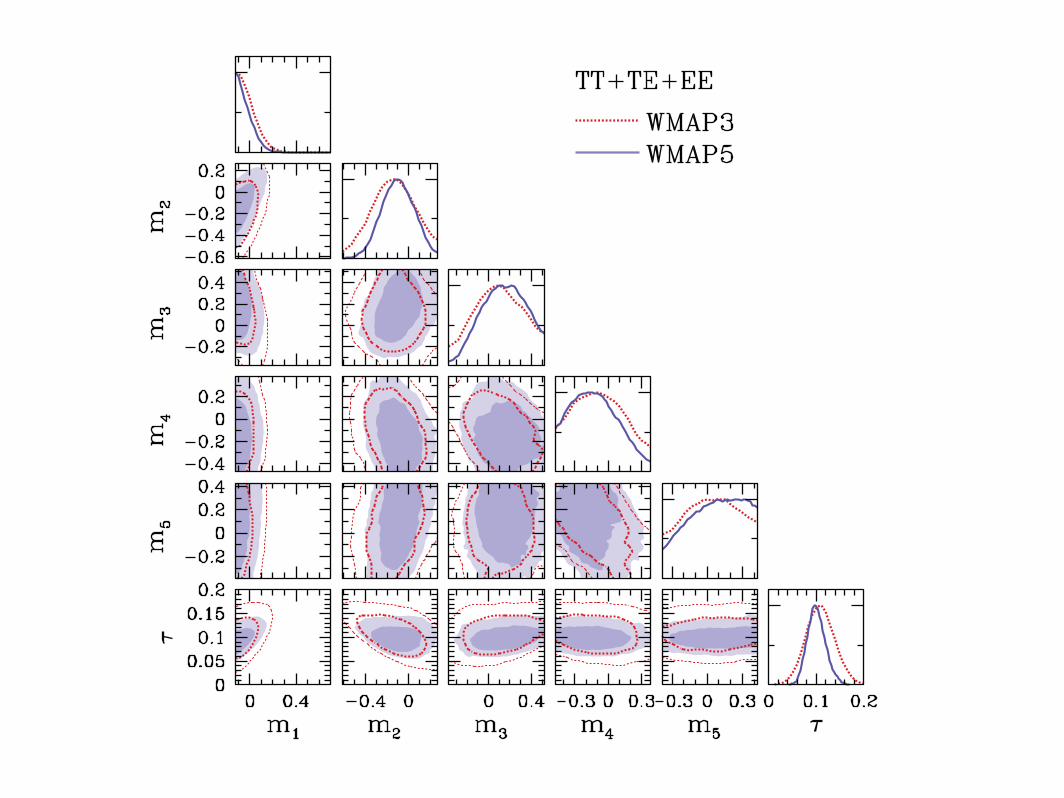
Fig. 1.— Marginalized 2D 68% and 95% CL contours for the optical depth to reionization (τ) and the amplitudes of the 5 lowest-varianceprincipal components of xe(z) (mµ, µ = 1−5). Panels along the diagonals show the 1D posterior probability distributions. Constraints areplotted for both 3-year (red dotted lines) and 5-year (blue shading, solid lines) WMAP data. In the left plot, only the low-" reionizationpeak in the E-mode polarization power spectrum is used for parameter constraints, and all parameters besides the 5 PC amplitudes and τare held fixed. For the constraints in the right plot, we use both temperature and polarization data and allow five additional parameters tovary: Ωbh

2, Ωch2, θA, As, and ns. The plot boundaries for the PC amplitudes correspond to physicality priors that exclude models thatare unable to satisfy 0 ≤ xe ≤ 1 for any combination of the higher-variance (µ ≥ 6) PCs.

effects of reionization on large-scale CMB polarization,so we obtain a very general parametrization of the reion-ization history at the expense of only a few additionalparameters.

The principal components are defined over a limitedrange in redshift, zmin < z < zmax, with xe = 0 atz > zmax and xe = 1 at z < zmin. We take zmin = 6,since the absence of Gunn-Peterson absorption in thespectra of quasars at z ! 6 indicates that the universe isnearly fully ionized at lower redshifts (Fan et al. 2006).In the MCMC analysis presented here, we always use thefive lowest-variance principal components of xe(z) withzmax = 30, constructed around a constant fiducial modelof xfid

e (z) = 0.15. The amplitudes of these componentsthen serve to parametrize general reionization historiesin the analysis of CMB polarization data. We refer thereader to Mortonson & Hu (2008a) for further discussionof these choices and the demonstration that five compo-nents suffice to describe the E-mode spectrum to betterthan cosmic variance precision.

We impose priors on the principal component ampli-tudes corresponding to physical values of the ionized frac-tion, 0 ≤ xe ≤ 1, according to the conservative approachof Mortonson & Hu (2008a). All excluded models areunphysical, but the models we retain are not necessarilystrictly physical. Finally, we neglect helium reionization,which is a small correction at the current level of preci-sion but will be more important for future analyses (e.g.,Colombo & Pierpaoli 2008).

3. OPTICAL DEPTH CONSTRAINTS

We examine the implications of the WMAP 5-yeardata for general models of reionization parametrized byprincipal components using a Markov Chain Monte Carloanalysis that mirrors our previous study of the 3-year

data in Mortonson & Hu (2008a). We consider con-straints from either large-scale polarization alone, withparameters that do not directly affect reionization fixedto values that fit the temperature data (“EE”), or fromthe full set of temperature and polarization data, varyingthe parameters of the “vanilla” ΛCDM model (baryondensity Ωbh2, cold dark matter density Ωch2, acous-tic scale θA, scalar amplitude As, and scalar spectraltilt ns) in addition to the reionization PC amplitudes(“TT+TE+EE”). In both cases, the total optical depthto reionization, τ , is a derived parameter.

The MCMC constraints on principal component am-plitudes and the derived optical depth for both of thesecases are plotted in Fig. 1, along with the previousconstraints from 3-year WMAP data (Mortonson & Hu2008a). While there are some improvements in all 5 ofthe individual components when considering EE alone,these changes are not as large as the improvement in theoptical depth constraint when all of the data are consid-ered. Adding both temperature data and extra parame-ters in going from EE only to TT+TE+EE has the neteffect of slightly strengthening constraints on the higherranked PC amplitudes, although there is very little ef-fect on τ . The additional constraining power for both3-year and 5-year data comes mainly from the measuredtemperature power spectrum at # ∼ 10 − 100, which ex-cludes models with additional Doppler effect contribu-tions due to narrow features in the ionization history(Mortonson & Hu 2008a).

Modeling reionization as an instantaneous transition atsome redshift zreion, Dunkley et al. (2008) estimate theoptical depth from the 5-year WMAP data to be τ =0.087±0.017, almost a factor of two more precise than theestimate from three years of data (Spergel et al. 2007).

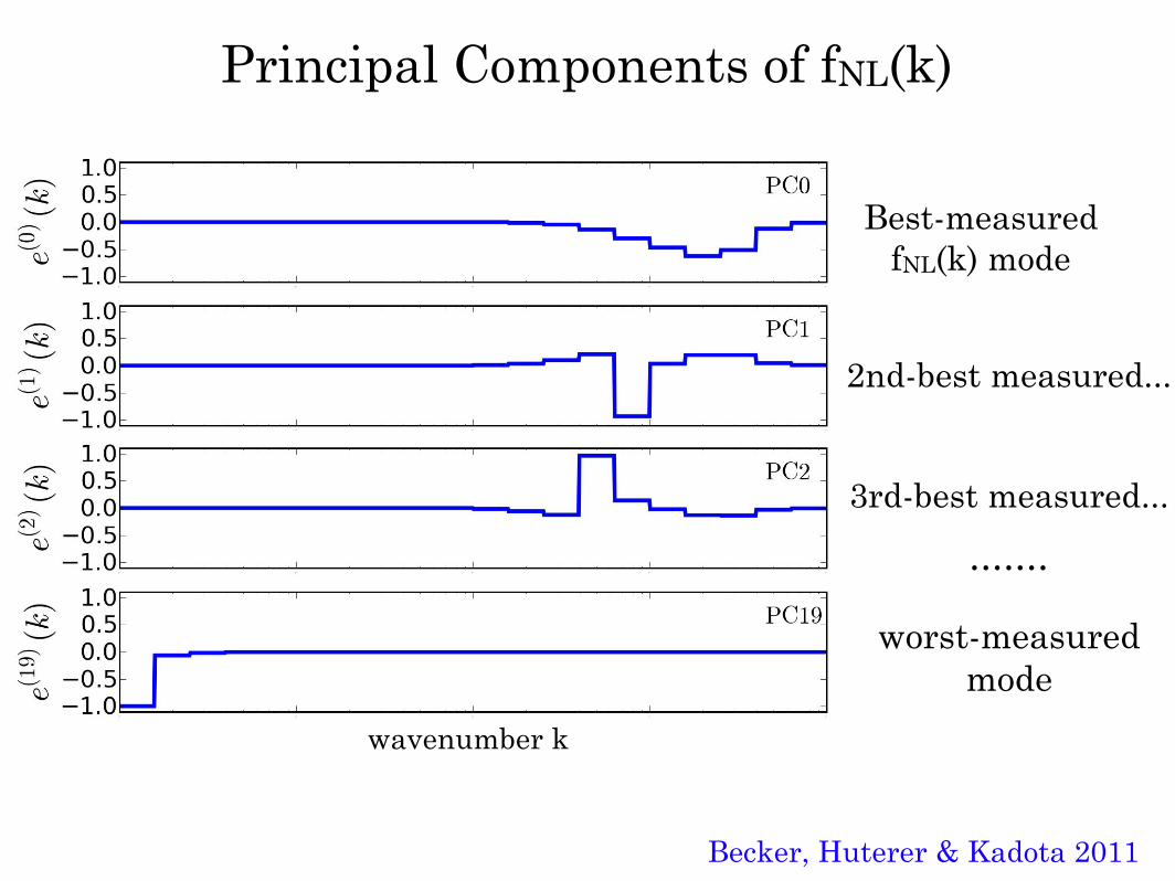
Figure 3: The first three, and the last (10th), principal component of fNL(k). The PCs, e(i)(k), arebasically eigenvectors of the covariance matrix for piecewise-constant values of fNL(k) in wavenum-ber bins uniformly distributed in log k, and are ordered from the best-measured one (i = 0), tothe worst-measured one (i = 9) for the assumed fiducial survey. [Kenji: Check the shape doesn’tchange by including more bins. My worry is it changes by including 15 bins instead of 10 bins. Itmeans 10 bins are not enough! This figure could be put in the earlier section because this fig is asort of important to illustrate the properties of our PCs.]

5.2 Principal components and relation to local and equilateral models

[Kenji: what’s the punchline of this subsection? What is the conclusion of this sectionimportant for? maybe we could put it in the discussion section by changing the title of thenext section to something like ’Discussion and Conclusion’?] [Dragan: Seems that PCsand cosines are some quantitative results in the paper, so I would put them in a separatesection (like this one) before D&C. I wrote an intro par here to motivate the PCs, whichbasically tell you what you measure. See comment below for the cosines result.]

[Dragan: (new par).] We now represent a general function fNL(k) in terms of principalcomponents (PCs). This decomposition is very convenient, as it tells us which particularmodes of fNL(k) are best or worst measured. The PCs will also enable us to measurethe overlap of our non-Gaussianity as specified by our generalized ansatz to the local andequilateral forms of non-Gaussianity.

It is rather straightforward to start from the covariance matrix for the piecewise con-stant parameters f i

NL and obtain the principal components (PCs) of fNL(k). The PCs are

– 12 –

Principal Components of fNL(k)

Best-measured fNL(k) mode

2nd-best measured...

3rd-best measured...

worst-measured mode

wavenumber k

Becker, Huterer & Kadota 2011

.......

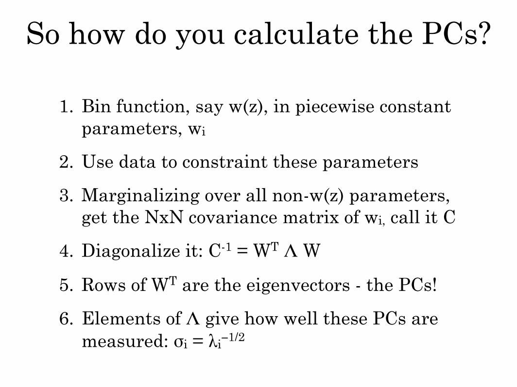
1. Bin function, say w(z), in piecewise constant parameters, wi

2. Use data to constraint these parameters

3. Marginalizing over all non-w(z) parameters, get the NxN covariance matrix of wi, call it C

4. Diagonalize it: C-1 = WT Λ W

5. Rows of WT are the eigenvectors - the PCs!

6. Elements of Λ give how well these PCs are measured: σi = λi

−1/2

So how do you calculate the PCs?

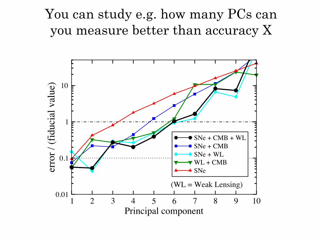
You can study e.g. how many PCs can you measure better than accuracy X

1 2 3 4 5 6 7 8 9 10Principal component

0.01

0.1

1

10

erro

r / (f

iduc

ial v

alue

)

SNe + CMB + WLSNe + CMBSNe + WLWL + CMBSNe

(WL = Weak Lensing)

Bayesian probability interprets the concept of probability as a measure of a state of knowledge, and not as a frequency.

One of the crucial features of the Bayesian view is that a probability can be assigned to a hypothesis, which is not possible under the frequentist view, where a hypothesis can only be rejected or not rejected.

Bayesian statistics

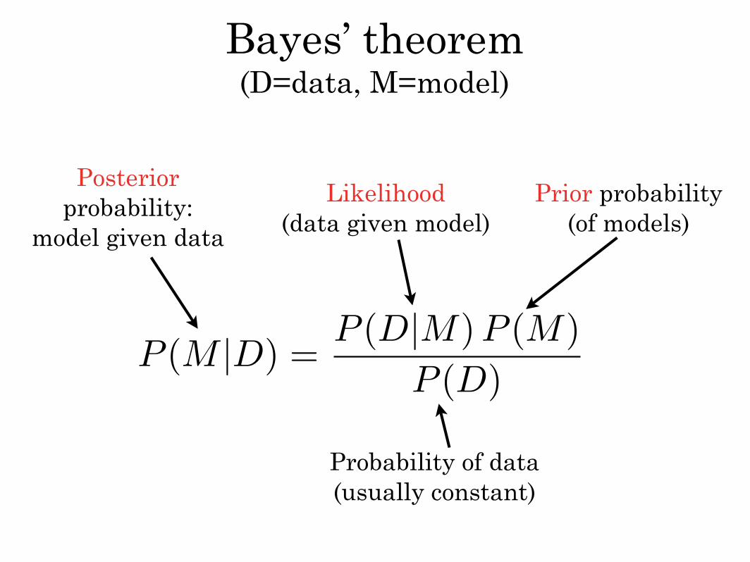
P (M |D) =P (D|M) P (M)

P (D)

Bayes’ theorem (D=data, M=model)

Posterior probability:

model given data

Likelihood(data given model)

Prior probability(of models)

Probability of data(usually constant)

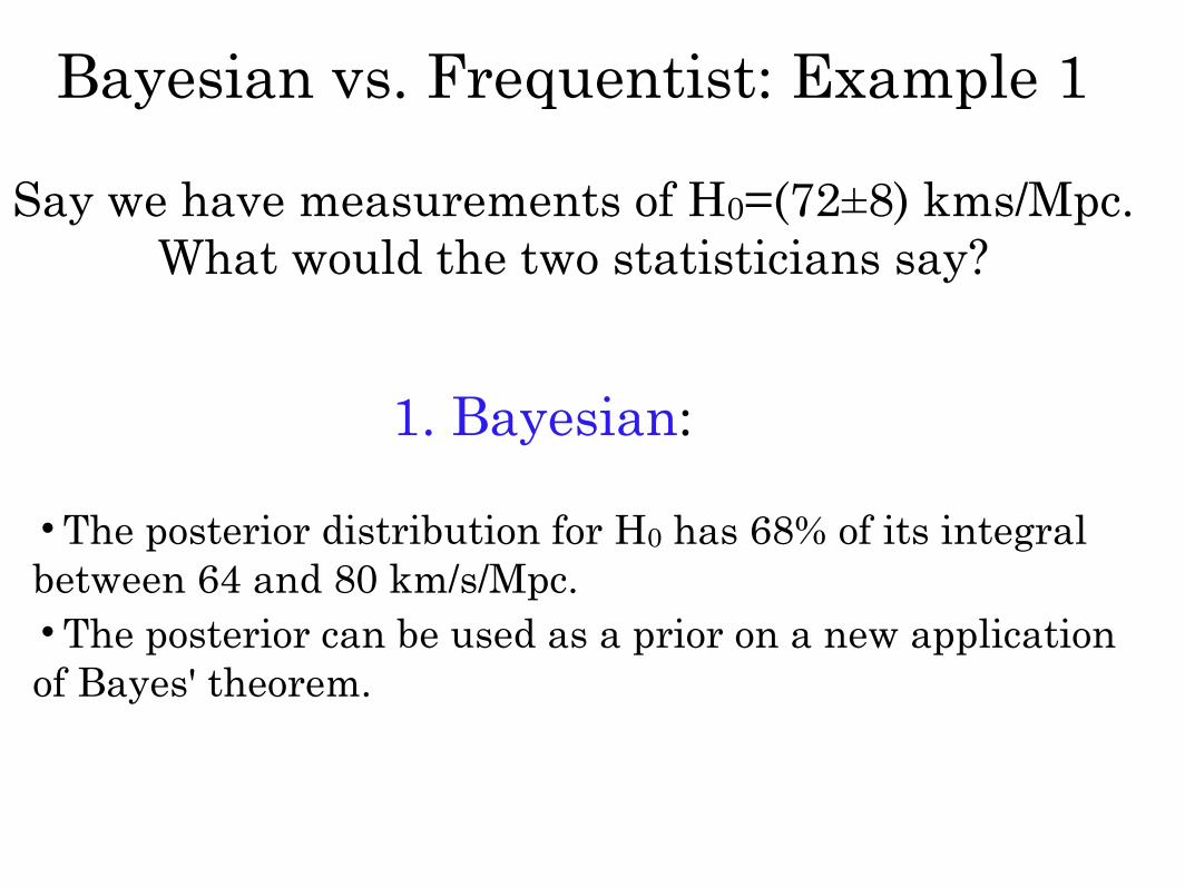
Say we have measurements of H0=(72±8) kms/Mpc.What would the two statisticians say?

•The posterior distribution for H0 has 68% of its integral between 64 and 80 km/s/Mpc. •The posterior can be used as a prior on a new application of Bayes' theorem.

1. Bayesian:

Bayesian vs. Frequentist: Example 1

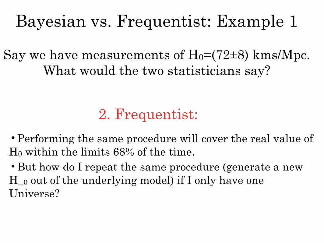
Say we have measurements of H0=(72±8) kms/Mpc.What would the two statisticians say?

•Performing the same procedure will cover the real value of H0 within the limits 68% of the time. •But how do I repeat the same procedure (generate a new H_0 out of the underlying model) if I only have one Universe?

2. Frequentist:


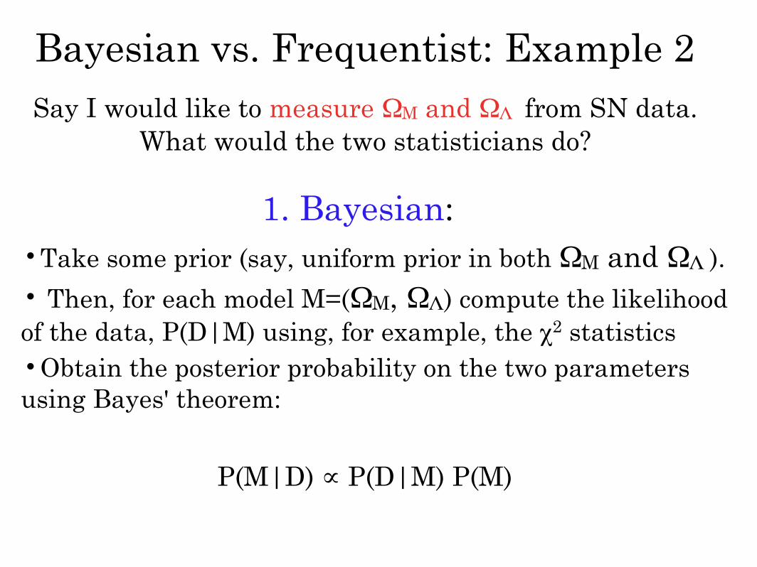
Say I would like to measure ΩM and ΩΛ from SN data. What would the two statisticians do?

•Take some prior (say, uniform prior in both ΩM and ΩΛ ).

• Then, for each model M=(ΩM, ΩΛ) compute the likelihood of the data, P(D|M) using, for example, the χ2 statistics•Obtain the posterior probability on the two parameters using Bayes' theorem:

1. Bayesian:

P(M|D) ∝ P(D|M) P(M)


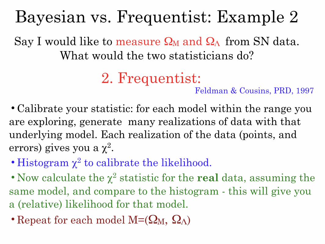
Say I would like to measure ΩM and ΩΛ from SN data. What would the two statisticians do?

•Calibrate your statistic: for each model within the range you are exploring, generate many realizations of data with that underlying model. Each realization of the data (points, and errors) gives you a χ2.

•Histogram χ2 to calibrate the likelihood.

•Now calculate the χ2 statistic for the real data, assuming the same model, and compare to the histogram - this will give you a (relative) likelihood for that model.

•Repeat for each model M=(ΩM, ΩΛ)

2. Frequentist:Feldman & Cousins, PRD, 1997


Statistics: philosophy

•When data are informative, Bayesian and frequentist approach will give very similar results

•But when data are ‘weak’, the two will generally differ

•No ‘right answer’ as to which one is better

•Given that we have 1 universe and cannot get arbitrary amount of data, Bayesian approach seems more appropriate

•In particular, Bayesian enables answering questions about model selection (e.g. is a dark energy model with w(z) a better fit to the data than w=const) A

•Also Bayesian enables easily adding new information (new data)

e.g. Trotta, arXiv:0804:4089

Markov Chain Monte Carlo

Avoiding the grid:Markov chain Monte Carlo

(MCMC)

•Say we’d like to constraint cosmological parameters using some CMB or LSS data

•We have ~10 parameters; say we consider 20 values in each parameter to get smooth contours

•→ 2010 (∼ 1013) parameter combinations

•CAMB and WMAP likelihood take seconds to run per model → a total of 100 million years CPU time

•A better strategy of the likelihood exploration is needed!

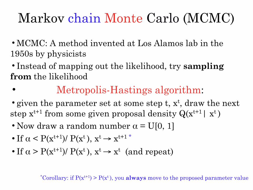
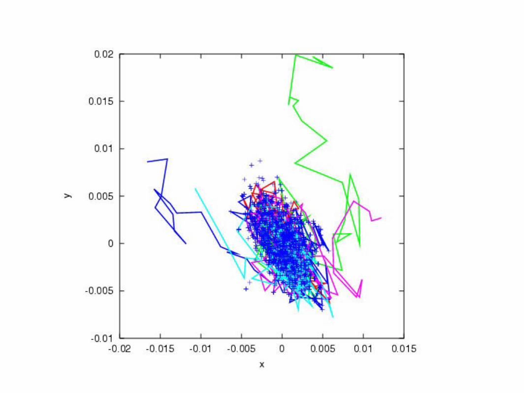
Markov chain Monte Carlo (MCMC)

•MCMC: A method invented at Los Alamos lab in the 1950s by physicists

•Instead of mapping out the likelihood, try sampling from the likelihood

• Metropolis-Hastings algorithm: •given the parameter set at some step t, xt, draw the next step xt+1 from some given proposal density Q(xt+1| xt )

•Now draw a random number α = U[0, 1]

•If α < P(xt+1)/ P(xt ), xt → xt+1 *

•If α > P(xt+1)/ P(xt ), xt → xt (and repeat)

*Corollary: if P(xt+1) > P(xt ), you always move to the proposed parameter value

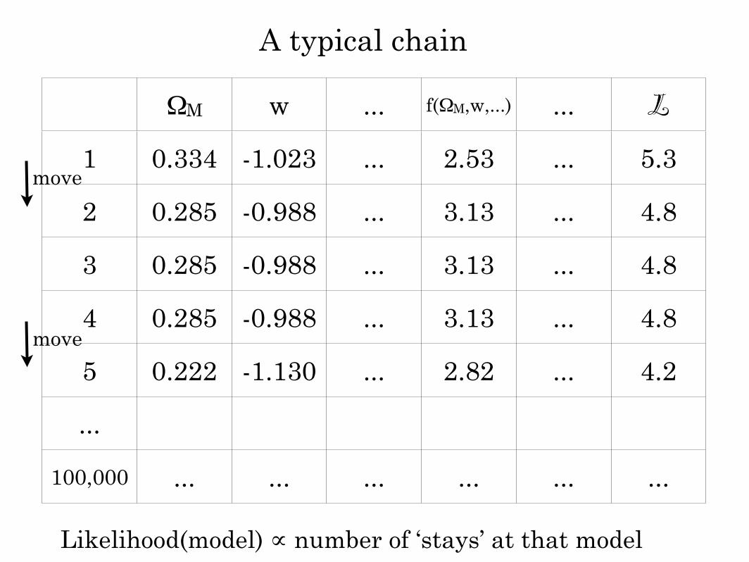
ΩM w ... f(ΩM,w,...) ... L

1 0.334 -1.023 ... 2.53 ... 5.3

2 0.285 -0.988 ... 3.13 ... 4.8

3 0.285 -0.988 ... 3.13 ... 4.8

4 0.285 -0.988 ... 3.13 ... 4.8

5 0.222 -1.130 ... 2.82 ... 4.2

...

100,000 ... ... ... ... ... ...

A typical chain

move

move

Likelihood(model) ∝ number of ‘stays’ at that model

Observational bounds on the cosmic radiation density 11

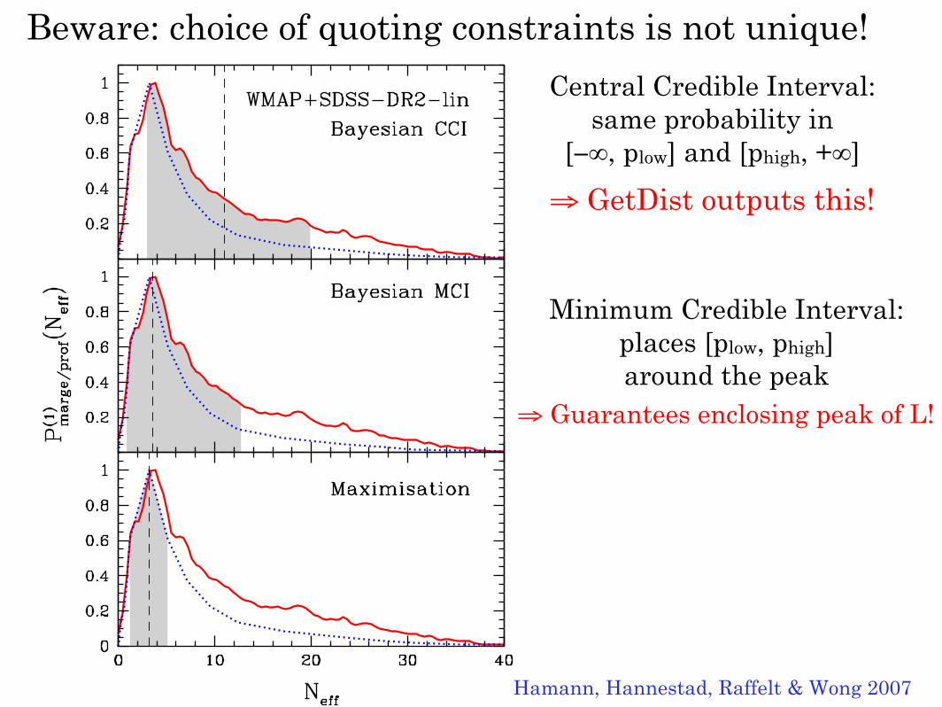
Figure 1. The 1D marginal (red/solid) and profile (blue/dotted) posteriors withrespect to Neff for our minimal model, the data set WMAP+SDSS-DR2-lin and tophat prior 0.2 ≤ h ≤ 2.0. The shaded regions are, from top to bottom, the Bayesian68% central credible interval, the 68% minimum credible interval, and the 1σ intervalderived from maximisation. The dashed vertical lines mark, from top to bottom,the posterior mean 〈Neff〉, the 1D marginal posterior mode N

(1)eff , and the global

best fit Neff .

“compressed.” It is common to map the posterior probability P (θ|x) onto a lower-

dimensional subspace by the process of marginalisation,

P (n)marge(θ

(n)) ∝∫

dθn+1 . . . dθN P (θ|x), (5.5)

where θ(n) = (θ1, . . . , θn) represents the parameters in the n-dimensional subspace.

Point estimates for θ(n) and credible regions may then be constructed from the marginal

posterior probability in analogy to section 5.3 above.

Marginalisation favours regions of parameter space that contain a large volumeof the probability density in the marginalised directions. This “volume effect” can

sometimes lead to counter-intuitive results, such as suppression of the probability density

for the global best fit parameters θ if they appear within sharp peaks or ridges that

contain little volume. Moreover, the concept of volume itself depends on the choice

Hamann, Hannestad, Raffelt & Wong 2007

Beware: choice of quoting constraints is not unique!

Central Credible Interval:same probability in

[−∞, plow] and [phigh, +∞]

⇒ GetDist outputs this!

Minimum Credible Interval:places [plow, phigh]around the peak

⇒ Guarantees enclosing peak of L!

Fisher Information Matrix

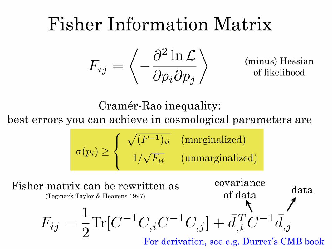
Fisher Information Matrix

Fij =−∂2 lnL

∂pi∂pj

Cramér-Rao inequality: best errors you can achieve in cosmological parameters are

σ(pi) ≥

(F−1)ii (marginalized)

1/√

Fii (unmarginalized)

Fisher matrix can be rewritten as (Tegmark Taylor & Heavens 1997)

Fij =12Tr[C−1C,iC

−1C,j ] + dT,i C−1d,j

datacovariance

of data

(minus) Hessian of likelihood

For derivation, see e.g. Durrer’s CMB book

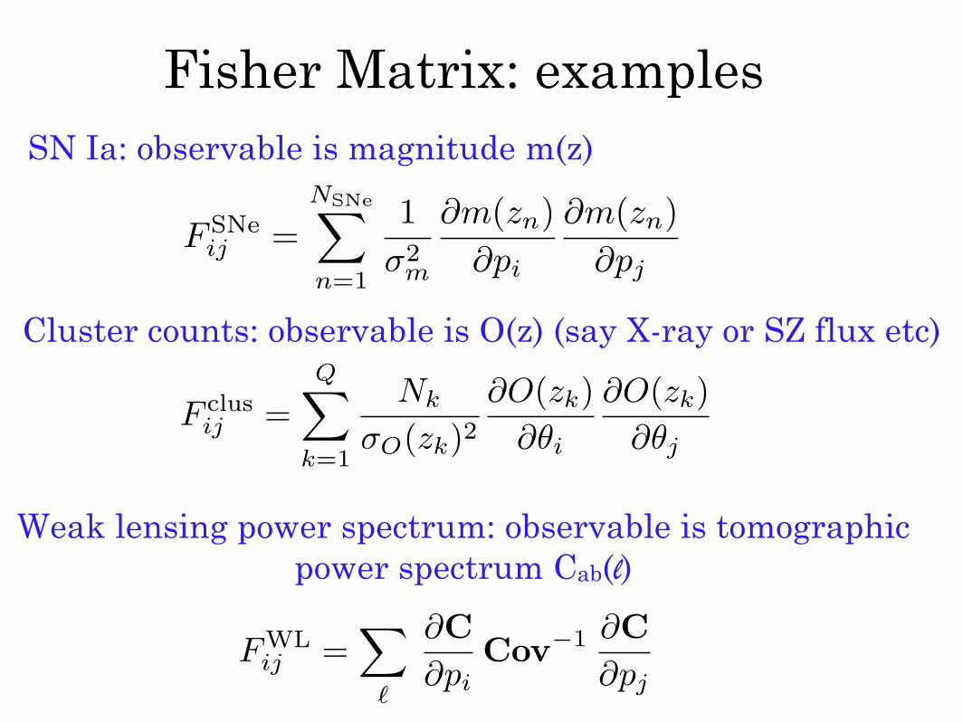
Fisher Matrix: examples

F SNeij =

NSNe

n=1

1σ2

m

∂m(zn)∂pi

∂m(zn)∂pj

SN Ia: observable is magnitude m(z)

Cluster counts: observable is O(z) (say X-ray or SZ flux etc)

Fclusij =

Q

k=1

Nk

σO(zk)2∂O(zk)

∂θi

∂O(zk)∂θj

Weak lensing power spectrum: observable is tomographic power spectrum Cab(l)

FWLij =

∂C∂pi

Cov−1 ∂C∂pj

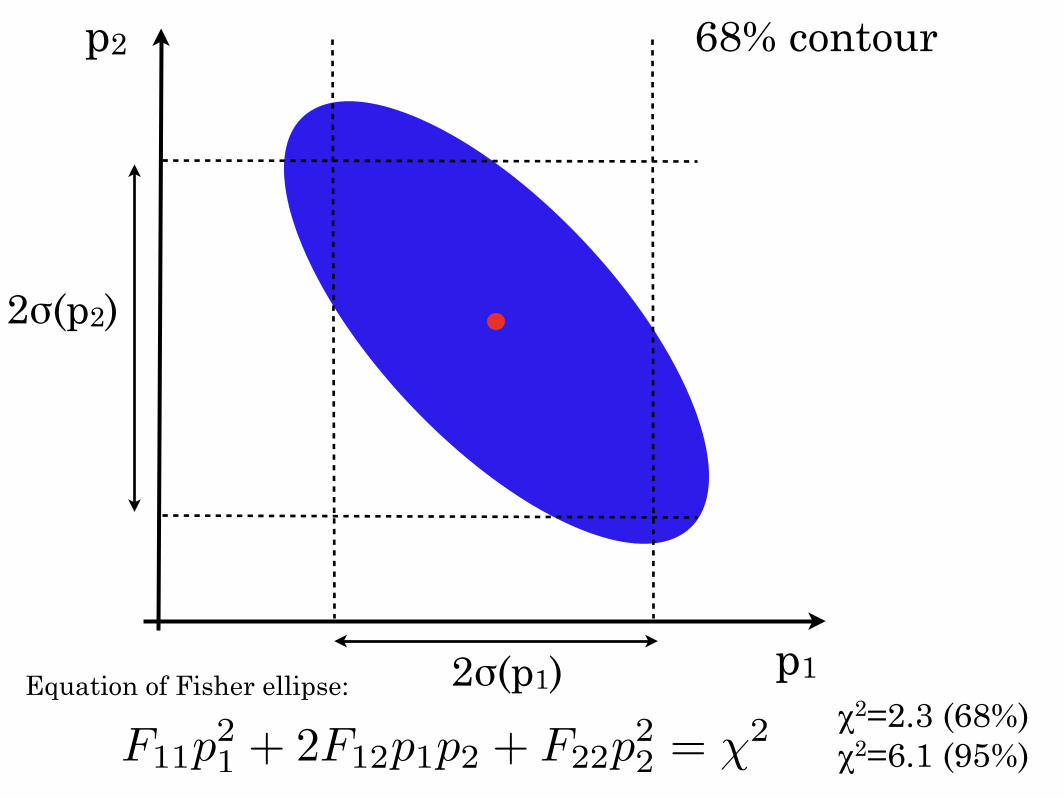
p1

p2

2σ(p1)

2σ(p2)

68% contour

F11p21 + 2F12p1p2 + F22p

22 = χ2

Equation of Fisher ellipse:χ2=2.3 (68%)χ2=6.1 (95%)

Fisher Matrix: facts

•Extremely useful tool for forecasting errors (and also Figures of Merit, in defining PCs, in the quadratic estimator method, etc)

•Easy to calculate: - only need one calculation of the observables for the fiducial model, and its derivatives wrt cosmological parameters

•Assumes that the likelihood (in parameters) is Gaussian: good approximation near the peak of likelihood (i.e. when the parameter errors are small)

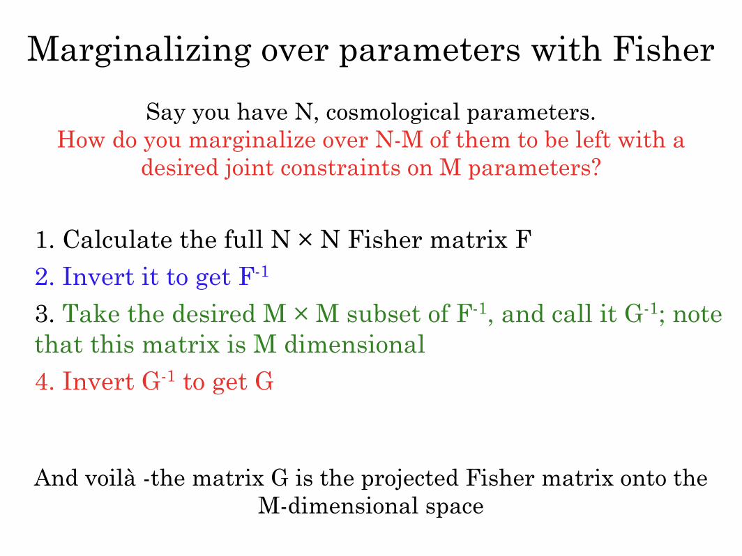
Marginalizing over parameters with Fisher

1. Calculate the full N × N Fisher matrix F2. Invert it to get F-1

3. Take the desired M × M subset of F-1, and call it G-1; note that this matrix is M dimensional4. Invert G-1 to get G

And voilà -the matrix G is the projected Fisher matrix onto theM-dimensional space

Say you have N, cosmological parameters. How do you marginalize over N-M of them to be left with a

desired joint constraints on M parameters?

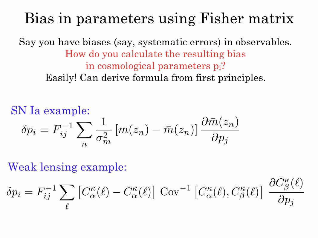
Bias in parameters using Fisher matrixSay you have biases (say, systematic errors) in observables.

How do you calculate the resulting bias in cosmological parameters pi?

Easily! Can derive formula from first principles.

Weak lensing example:

SN Ia example:

δpi = F−1ij

Cκ

α()− Cκα()

Cov−1

Cκ

α(), Cκβ ()

∂Cκβ ()

∂pj

δpi = F−1ij

n

1σ2

m

[m(zn)− m(zn)]∂m(zn)

∂pj

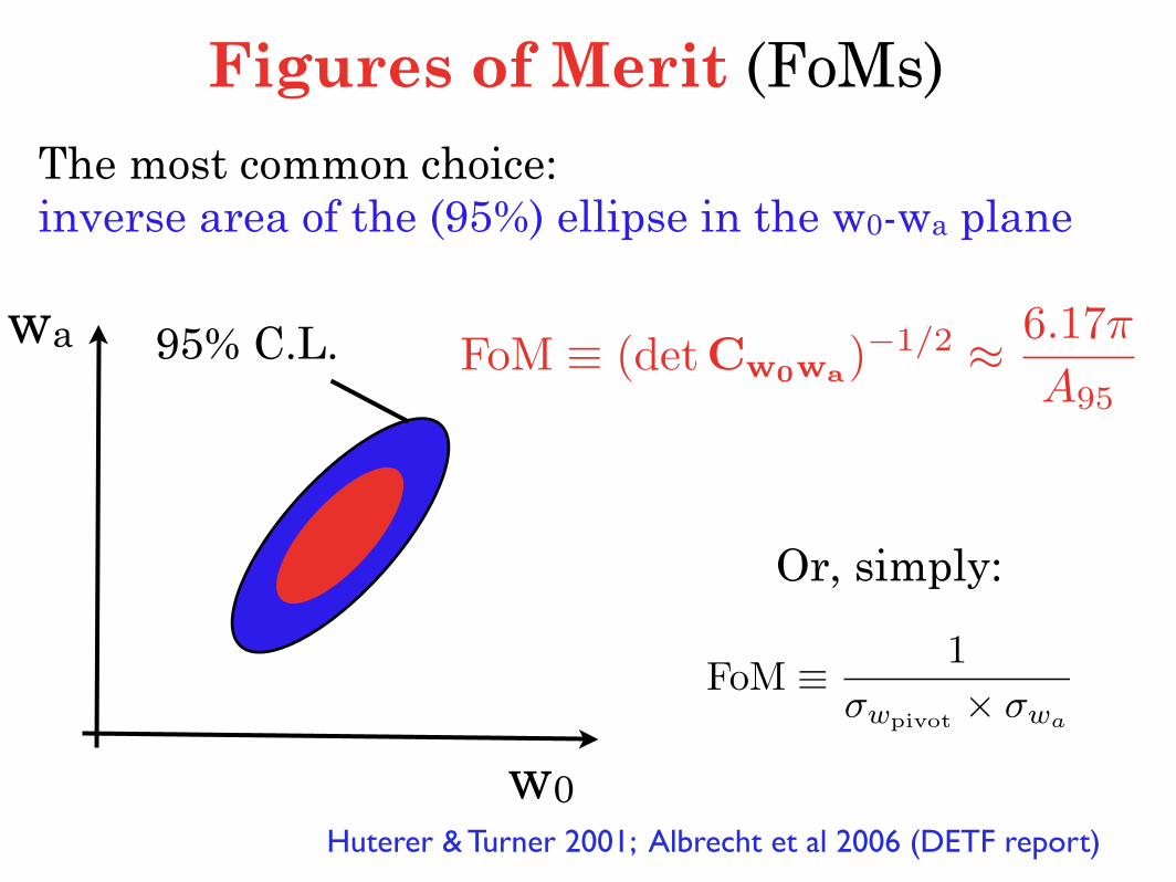
Figures of Merit (FoMs)

w0

wa 95% C.L.

The most common choice:inverse area of the (95%) ellipse in the w0-wa plane

Or, simply:

FoM ≡ 1σwpivot × σwa

FoM ≡ (detCw0wa)−1/2 ≈ 6.17π

A95

Huterer & Turner 2001; Albrecht et al 2006 (DETF report)

Future/current ratio

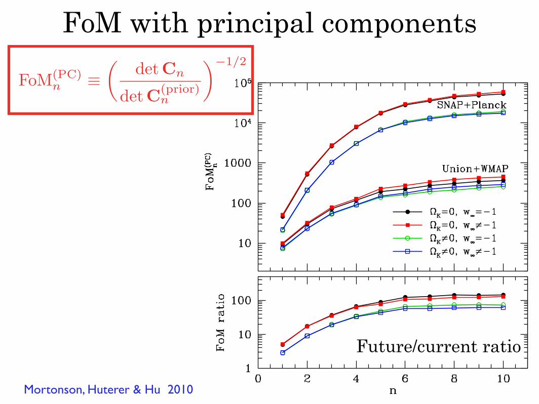
FoM(PC)n ≡

detCn

detC(prior)n

−1/2

Mortonson, Huterer & Hu 2010

FoM with principal components


Topic I: Discovery of the Accelerating Universe

Recommended reading:

• “Measurements of the cosmological parameters ΩM and Λ from 42 high-redshift super-novae”, S. Perlmutter et al. (The Supernova Cosmology Project), Astrophysical Journal517, 565 (1999) — a classic.

• “Supernovae, Dark Energy, and the Accelerating Universe”, S. Perlmutter, Physics Today,April 2003 — very nice popular account.

• “Measuring Cosmology with Supernovae”, Saul Perlmutter and Brian P. Schmidt, Super-novae & Gamma Ray Bursts, K. Weiler, Ed., Springer, Lecture Notes in Physics, astro-ph/0303428 — intermediate level overview.

• “Improved Dark Energy Constraints from ∼ 100 New CfA Supernova Type Ia LightCurves”, M. Hicken et al., arXiv:0901:4804 — one of latest and greatest SN Ia data sets.

• “Dark Energy and the Accelerating Universe”, J. Frieman, M. Turner and D. Huterer, Ann.Rev. Astron. Astrophys. 46, 385 (2008)(http://huterer8.physics.lsa.umich.edu/~huterer/Papers/ARAA_DE.pdf)— a review of DE for a general-practice physicist or astronomer.

Introduction. Type Ia supernovae are interesting objects. They have been studied exten-sively by the famous American-Swiss astronomer Fritz Zwicky (there is a notable paper by Baadeand Zwicky from 1934); Zwicky gave them their name. They have been known to have nearlyuniform luminosity; this feature is easily understood from the currently favored explanation forthe physics of these events: these are white dwarf stars accreting matter from a companion,going over the Chandrasekhar limit, and undergoing explosion.

Explosions of type Ia supernovae are extremely luminous events that can be seen across theobservable universe. At their peak, SNe Ia can be as luminous as the entire galaxy in which theyreside.

Standard candles. It is very difficult to measure distances in astronomy. You can get red-shift of an object from its spectrum, but how do you get the distance? There are many empirical— and uncertain — ways to do so (surface brightness fluctuations, period-luminosity relation ofCepheids, proper motions, etc). Typically, astronomers construct an unwieldy “distance ladder”to measure distance to a distant galaxy: they use some of these relations (say, proper motions)to calibrate distances to more nearby objects, then go from those objects to more distant onesusing other relations that work better in that distance regime. This procedure is clearly notrobust.

A “standard candle” is a hypothetical object that has a fixed luminosity (that is, fixed intrinsicpower that it radiates). Having a standard candle would be useful since then you could inferdistances from objects just by using the inverse square law, f = L/(4πd2), by measuring the fluxf and knowing the luminosity L from the standard candle property. In fact, you don’t even toknow the luminosity of the standard candle to be able to infer relative distances to objects – allyou need to know that thus luminosity is the same for all objects.

1

The fact that SNe Ia can potentially be used as a standard candle has been realized longago (at least as far back as the 1970, as far as I know). Briefly, SNe Ia are extremely brightexplosions that are presumed to be cases when a white dwarf accretes matter from a (binary)companion, and exceeds the Chandrasekhar mass limit and explodes. These SN type is definedby the absence of Hydrogen in their spectra, but the unmistakable presence of a Silicon line at6150 Angstroms.

Finding SNe. However, a real problem was scheduling telescopes to detect and “follow-up”SNe that are discovered. Basically, if you point a telescope at a galaxy and wait for the SN togo off, you will wait an average of 500 years. There has been a program in the 1980s to do that(Norgaard-Nielsen, 1989) and it discovered only one SN, and after the peak!

A real breakthrough came in the 1990s when two teams of SN researchers, Supernova Cos-mology Project (SCP; lead by Saul Perlmutter) and High-z Supernova Team (Highz; lead, at thetime, by Brian Schmidt) made careful use of world’s most powerful telescope working in concertto discover and follow up SNe, essentially guaranteeing to funding agencies that they will findbatches of SNe in each run.

Some of the early results came out in 1997, which paradoxically indicated that the universe ismatter-dominated and consistent with being flat. But those early measurements were based ononly 7 high-z SNe and had large errors. The definitive results came out in 1998 (High-z team)and 1999 (SCP, though they had results earlier) and indicated that the universe is dominatedby a component with negative pressure.

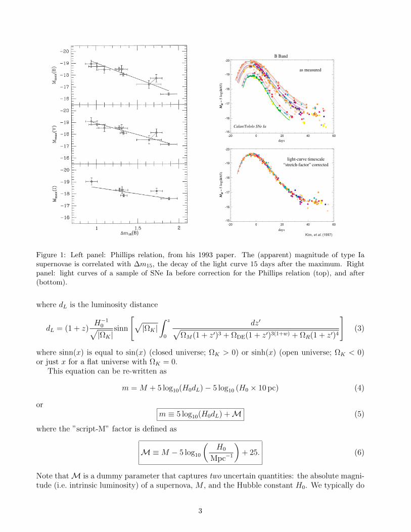
Broader is brighter. Another major breakthrough came in 1993 by Mark Phillips (as-tronomer working in Chile). He noticed that the intrinsic SN brightness (or, SN luminosity)is correlated with the decay time of SN light curve. Phillips considered the following quantity:∆m15, the decay of the light curve 15 days after the maximum. He found that ∆m15 is stronglycorrelated with the intrinsic brightness of SNe. In other words, he found the “Phillips relation”which roughly goes as

Broader is brighter.

(see left panel of Fig. 1). Phillips found that the intrinsic dispersion of SNe, which is ∼ 0.5 mag-nitudes (depending on which band you look at, etc), can be brought down to ∼ 0.2 magnitudesonce you correct each SN luminosity by this relation, using of course its measured ∆m15. Inastronomers’ language, the Phillips relation is

Mmax = a+ b (∆m15) (1)

where mmax is the absolute magnitude of SN, a and b are some constants, and the dispersion inthis relation around the mean is small as mentioned above.

The Phillips relation was the second key breakthrough that enabled SNe Ia to achieve preci-sion needed to probe dark energy.

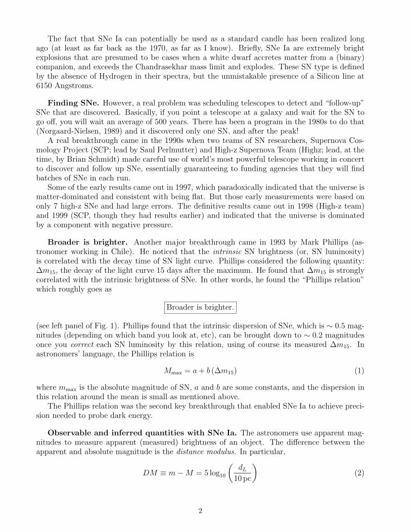
Observable and inferred quantities with SNe Ia. The astronomers use apparent mag-nitudes to measure apparent (measured) brightness of an object. The difference between theapparent and absolute magnitude is the distance modulus. In particular,

DM ≡ m−M = 5 log10

(dL

10 pc

)(2)

2

1993ApJ...413L.105P

-20 0 20 40 60-15

-16

-17

-18

-19

-20

-20 0 20 40 60-15

-16

-17

-18

-19

-20

B Band

as measured

light-curve timescale“stretch-factor” corrected

days

MB

– 5

log(

h/65

)

days

MB

– 5

log(

h/65

)

Calan/Tololo SNe Ia

Kim, et al. (1997)

Figure 1: Left panel: Phillips relation, from his 1993 paper. The (apparent) magnitude of type Iasupernovae is correlated with ∆m15, the decay of the light curve 15 days after the maximum. Rightpanel: light curves of a sample of SNe Ia before correction for the Phillips relation (top), and after(bottom).

where dL is the luminosity distance

dL = (1 + z)H−1

0√|ΩK |

sinn

[√|ΩK |

∫ z

0

dz′√ΩM(1 + z′)3 + ΩDE(1 + z′)3(1+w) + ΩR(1 + z′)4

](3)

where sinn(x) is equal to sin(x) (closed universe; ΩK > 0) or sinh(x) (open universe; ΩK < 0)or just x for a flat universe with ΩK = 0.

This equation can be re-written as

m = M + 5 log10(H0dL)− 5 log10 (H0 × 10 pc) (4)

orm ≡ 5 log10(H0dL) +M (5)

where the ”script-M” factor is defined as

M≡M − 5 log10

(H0

Mpc−1

)+ 25. (6)

Note thatM is a dummy parameter that captures two uncertain quantities: the absolute magni-tude (i.e. intrinsic luminosity) of a supernova, M , and the Hubble constant H0. We typically do

3

Supernova Cosmology Project

34

36

38

40

42

44

WM=0.3, WL=0.7

WM=0.3, WL=0.0

WM=1.0, WL=0.0

m-M

(m

ag)

High-Z SN Search Team

0.01 0.10 1.00z

-1.0

-0.5

0.0

0.5

1.0

D(m

-M)

(mag)

0.0 0.5 1.00.0

0.5

1.0

1.5

FlatBAO

CM

B

SNe

Supernova Cosmology Project

Kowalski, et al., Ap.J. (2008)

m

Union 08SN Ia

compilation

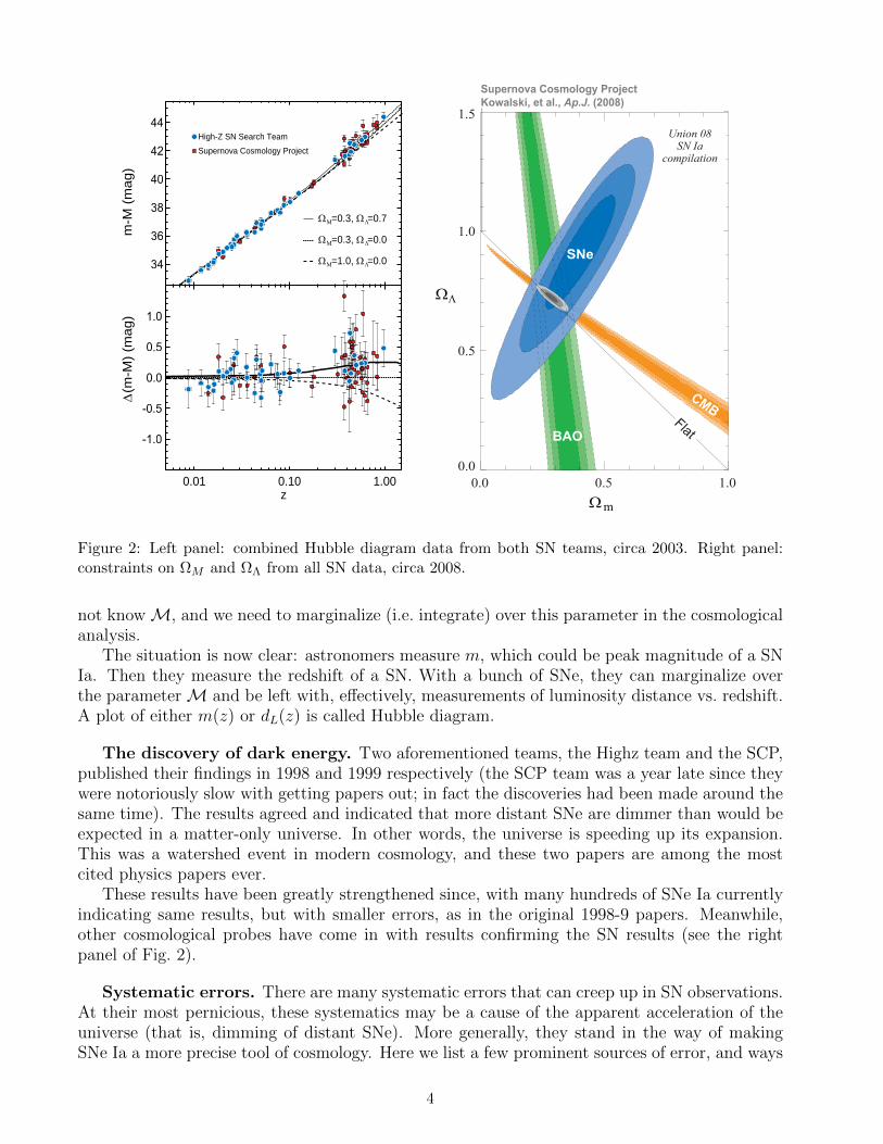
Figure 2: Left panel: combined Hubble diagram data from both SN teams, circa 2003. Right panel:constraints on ΩM and ΩΛ from all SN data, circa 2008.

not knowM, and we need to marginalize (i.e. integrate) over this parameter in the cosmologicalanalysis.

The situation is now clear: astronomers measure m, which could be peak magnitude of a SNIa. Then they measure the redshift of a SN. With a bunch of SNe, they can marginalize overthe parameterM and be left with, effectively, measurements of luminosity distance vs. redshift.A plot of either m(z) or dL(z) is called Hubble diagram.

The discovery of dark energy. Two aforementioned teams, the Highz team and the SCP,published their findings in 1998 and 1999 respectively (the SCP team was a year late since theywere notoriously slow with getting papers out; in fact the discoveries had been made around thesame time). The results agreed and indicated that more distant SNe are dimmer than would beexpected in a matter-only universe. In other words, the universe is speeding up its expansion.This was a watershed event in modern cosmology, and these two papers are among the mostcited physics papers ever.

These results have been greatly strengthened since, with many hundreds of SNe Ia currentlyindicating same results, but with smaller errors, as in the original 1998-9 papers. Meanwhile,other cosmological probes have come in with results confirming the SN results (see the rightpanel of Fig. 2).

Systematic errors. There are many systematic errors that can creep up in SN observations.At their most pernicious, these systematics may be a cause of the apparent acceleration of theuniverse (that is, dimming of distant SNe). More generally, they stand in the way of makingSNe Ia a more precise tool of cosmology. Here we list a few prominent sources of error, and ways

4

in which they are controlled:

• Extinction: there is dust between SN and dust (remember, some of them are thousandsof Mpc away!); is it possible that they appear dimmer simply because of extinction andnot dark energy? Well, there are ways to control (and correct for) extinction, basically bylooking at SNe in different colors. But also, if extinction were to be responsible for theappearance of dimming, then you’d expect more distant SNe to dim more, without limit.In fact, a “turnover” in the SN Hubble diagram has been observed - basically a signatureof universe being matter dominated at high z. This turnover cannot easily be explained byextinction.

• Evolution: is it possible that SNe evolve, so that you are seeing a different population athigher redshift that simply is intrinsically dimmer (violating the assumption of a standardcandle)? Well, SNe Ia do not own a “cosmic clock” by which they say “oops, 5 billion yearsfrom Big Bang, time to get brighter”. Rather, they respond to their local environment, inaddition to being ruled by physics of accretion/explosion. So, by observing various signa-ture, in particular in SN spectra, researchers can identify local environmental conditions,and even go so far to compare only like-to-like SNe (resulting, potentially, in several Hub-ble diagrams, one for each subspecies). First such divisions have been made recently, andindicate that DE results are insensitive to what subspecies of SNe is used to obtain them.

• Typing: is it possible that non-Ia supernovae have crept in the samples used for dark energyanalysis? Well this question is easy to answer: type Ia supernova possess a characteristicSilicon 6150 angstrom line (in rest frame), and this line, and a few others, are telltale signsof SNe Ia. This question, however, becomes more relevant for SN surveys which cannotafford to take spectra of all SNe (for example the LSST for most of their SNe, or the DarkEnergy Survey for 75% of their SNe). Then one must exercise a lot of care in studying thelight curves and trying to establish whether or not a given SN is SN Ia.

• K-corrections: As SNe Ia are observed at larger and larger redshifts, their light is shiftedto longer wavelengths. Since astronomical observations are normally made in fixed bandpasses on Earth, corrections need to be applied to account for the differences caused by thespectrum shifting within these band passes. These corrections take the form of integratingthe spectrum of an SN over the relevant band passes, shifting the SN spectrum to thecorrect redshift, and re-integrating.

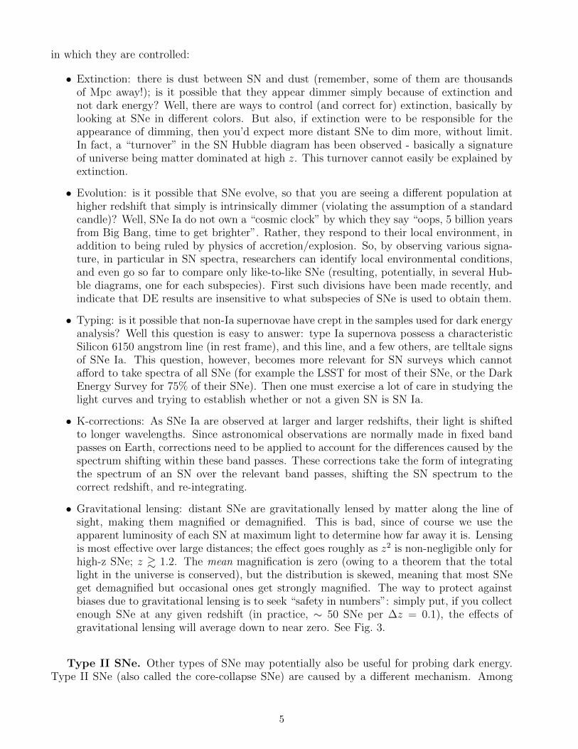
• Gravitational lensing: distant SNe are gravitationally lensed by matter along the line ofsight, making them magnified or demagnified. This is bad, since of course we use theapparent luminosity of each SN at maximum light to determine how far away it is. Lensingis most effective over large distances; the effect goes roughly as z2 is non-negligible only forhigh-z SNe; z & 1.2. The mean magnification is zero (owing to a theorem that the totallight in the universe is conserved), but the distribution is skewed, meaning that most SNeget demagnified but occasional ones get strongly magnified. The way to protect againstbiases due to gravitational lensing is to seek “safety in numbers”: simply put, if you collectenough SNe at any given redshift (in practice, ∼ 50 SNe per ∆z = 0.1), the effects ofgravitational lensing will average down to near zero. See Fig. 3.

Type II SNe. Other types of SNe may potentially also be useful for probing dark energy.Type II SNe (also called the core-collapse SNe) are caused by a different mechanism. Among

5

Safety in numbers 3

the implications for cosmological parameter determina-tion.

3. SAFETY IN NUMBERS

3.1. Perfect Standard Candles

We begin with an idealized experiment: a large sampleof perfect standard candles at high redshift. Withoutlensing, these would all be observed to have the samebrightness: a delta function PDF (normalized at µ =1). We now add in the effects of gravitational lensing,which both contributes a width to the observed PDF,and shifts the mode of the PDF to slightly demagnifiedvalues. As already emphasized, the non-Gaussian lensingPDF preserves the mean:

〈µ〉 =

∫dµ µP (µ) = 1. (1)

This crucial property implies that, for sufficiently highnumbers of observed high-redshift standard candles at agiven z, the average brightness (in flux) will converge tothe appropriate, unlensed brightness. It is to be noted,however, that the second moment of the lensing PDFdoesn’t necessarily converge. For the case of point-masslenses, the probability at high magnification falls off as1/µ3, and so the contribution to the second moment isgiven by:

⟨µ2

⟩=

∫dµ µ2P (µ) ∝

∫dµ/µ, (2)

which diverges logarithmically at high magnification,1

emphasizing the non-Gaussian nature of the PDFs.It is to be expected that the effects of non-Gaussianity

will be mitigated by observing sufficient numbers of SNe,and more fully sampling the lensing PDFs. With this inmind, we define PN (µ) as the lensing magnification PDFfor the mean magnification of a sample of N standardcandles (at a fixed redshift). We calculate P1(µ) via theSUM code. The distribution for higher numbers of stan-dard candles can then be calculated recursively:

PN (µ)=

∫∫dµ dµ′ PN−1(µ)P1(µ

′)δ

(µ − (N − 1)µ + µ′

N

),(3)

=N

∫dµ PN−1(µ)P1(Nµ − (N − 1)µ). (4)

This recursion becomes particularly straightforward us-ing spectral methods. Defining P1(k) as the Fouriertransform of the lensing PDF P1(µ1), the convolutionbecomes

PN (µ) = (2π)(N−2)/2N

∫dk PN

1 (k) e−ikNµ. (5)

As expected, the convolution (eq. 4 or 5) preserves thenormalization and mean of the distribution, and the vari-ance shrinks as 1/N . This formula reduces to a simpleexpression in the case of Gaussian or log-normal proba-bilities (see Appendix A).

1 In practice this is mitigated by effects such as finite sourcesize and obscuration. If the second moment does diverge, then thedistribution of observed brightnesses of large numbers of standardcandles does not necessarily converge to a Gaussian distributionby the central limit theorem, and statistical intuition based uponnormal statistics could lead us astray.

Fig. 1.— Effective lensing magnification distributions for mul-tiple perfect standard candles, at z = 1.5 in a ΛCDM concor-dance cosmology. As more sources are observed the distributionapproaches a Gaussian, and eventually converges on a δ-functionat the unlensed magnification, µ = 1.

The distributions at z = 1.5, for various values of N ,are shown in Figure 1. Note that even for as many as50 SNe averaged together, the resulting distribution inmagnification is still visibly asymmetric. This is a resultof the high-magnification tail possessed by the lensingdistributions. Figure 2 displays the shift of the mode ofthe distribution, as increasing numbers of SNe are ob-served. As expected, the curve asymptotes (slowly) toa value of 1, since the mean of the PDFs is always pre-served, and for large numbers of SNe the PDF should bewell sampled.

Figures 3 and 4 display the variance of the multiple SNlensing PDFs, as a function of the number of SNe. Sincewe are restricting our attention to smoothly clustereddark matter (as opposed to point masses like MACHOs;see Amanullah (2003) for a treatment of that case), thevariance for P1(µ) remains well-defined and finite. Thedifference between σ and the full width at half maxi-mum (FWHM) determination of the width is further ev-idence of the non-Gaussianity of the underlying lensingdistribution: for a perfect Gaussian, σ = FWHM/2.36.For N = 1, the standard deviation is 1.61 times theFWHM/2.36. By N = 50, this factor has gone downto 1.35, indicating a more Gaussian-like distribution.

3.2. Sources with intrinsic luminosity dispersion

If the sources were perfectly calibrated candles, thenthe distribution of observed fluxes would exactly mirrorthose shown in Figure 1 (i.e., reflect only the lensing mag-nification suffered during propagation). However, astro-nomical sources, even calibrated candles such as TypeIa supernovae, retain some intrinsic variation in theirluminosity. This gives an innate a priori fuzziness inthe distance-redshift relation, and the observed relationis thus a convolution of both the intrinsic and lensingflux distributions. In other words, the distribution ofobserved flux, F , is given by

P (F )=

∫dF0

∫dµ pint(F0) plens(µ) δ(F − F0µ) (6)

=

∫dµ

µpint

(F

µ

)plens(µ), (7)

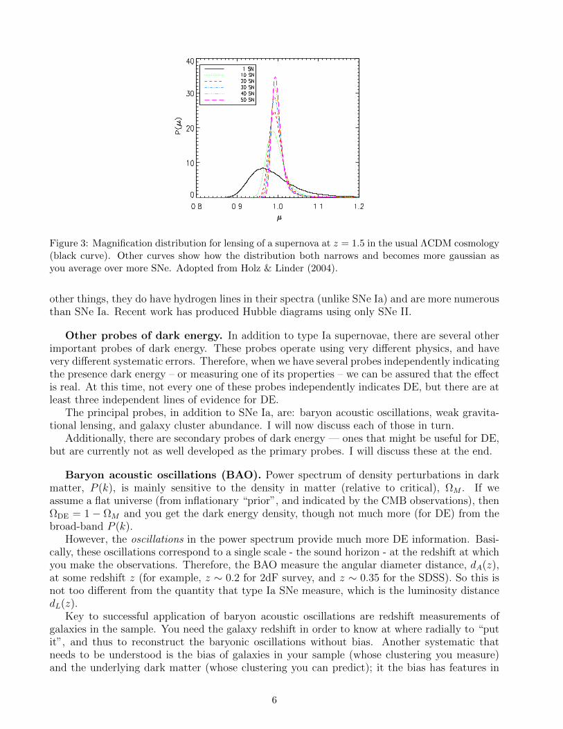
Figure 3: Magnification distribution for lensing of a supernova at z = 1.5 in the usual ΛCDM cosmology(black curve). Other curves show how the distribution both narrows and becomes more gaussian asyou average over more SNe. Adopted from Holz & Linder (2004).

other things, they do have hydrogen lines in their spectra (unlike SNe Ia) and are more numerousthan SNe Ia. Recent work has produced Hubble diagrams using only SNe II.

Other probes of dark energy. In addition to type Ia supernovae, there are several otherimportant probes of dark energy. These probes operate using very different physics, and havevery different systematic errors. Therefore, when we have several probes independently indicatingthe presence dark energy – or measuring one of its properties – we can be assured that the effectis real. At this time, not every one of these probes independently indicates DE, but there are atleast three independent lines of evidence for DE.

The principal probes, in addition to SNe Ia, are: baryon acoustic oscillations, weak gravita-tional lensing, and galaxy cluster abundance. I will now discuss each of those in turn.

Additionally, there are secondary probes of dark energy — ones that might be useful for DE,but are currently not as well developed as the primary probes. I will discuss these at the end.

Baryon acoustic oscillations (BAO). Power spectrum of density perturbations in darkmatter, P (k), is mainly sensitive to the density in matter (relative to critical), ΩM . If weassume a flat universe (from inflationary “prior”, and indicated by the CMB observations), thenΩDE = 1 − ΩM and you get the dark energy density, though not much more (for DE) from thebroad-band P (k).

However, the oscillations in the power spectrum provide much more DE information. Basi-cally, these oscillations correspond to a single scale - the sound horizon - at the redshift at whichyou make the observations. Therefore, the BAO measure the angular diameter distance, dA(z),at some redshift z (for example, z ∼ 0.2 for 2dF survey, and z ∼ 0.35 for the SDSS). So this isnot too different from the quantity that type Ia SNe measure, which is the luminosity distancedL(z).

Key to successful application of baryon acoustic oscillations are redshift measurements ofgalaxies in the sample. You need the galaxy redshift in order to know at where radially to “putit”, and thus to reconstruct the baryonic oscillations without bias. Another systematic thatneeds to be understood is the bias of galaxies in your sample (whose clustering you measure)and the underlying dark matter (whose clustering you can predict); it the bias has features in

6

scale, then the systematic errors creep in.Future surveys that plan to mine this method typically propose measuring redshifts of millions

of galaxies, and the goal is to go deep (z ∼ 1, and beyond) and have wide angular coverage aswell.

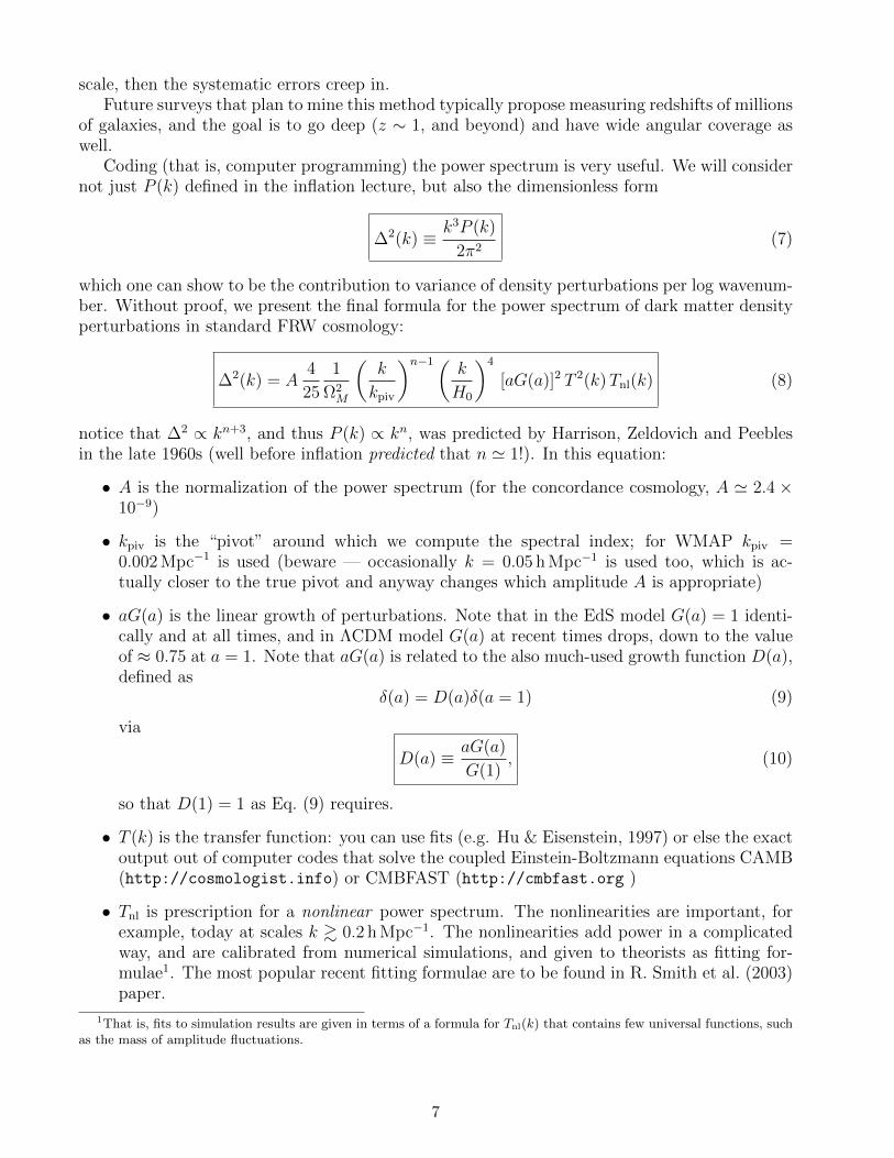
Coding (that is, computer programming) the power spectrum is very useful. We will considernot just P (k) defined in the inflation lecture, but also the dimensionless form

∆2(k) ≡ k3P (k)

2π2(7)

which one can show to be the contribution to variance of density perturbations per log wavenum-ber. Without proof, we present the final formula for the power spectrum of dark matter densityperturbations in standard FRW cosmology:

∆2(k) = A4

25

1

Ω2M

(k

kpiv

)n−1(k

H0

)4

[aG(a)]2 T 2(k)Tnl(k) (8)

notice that ∆2 ∝ kn+3, and thus P (k) ∝ kn, was predicted by Harrison, Zeldovich and Peeblesin the late 1960s (well before inflation predicted that n ' 1!). In this equation:

• A is the normalization of the power spectrum (for the concordance cosmology, A ' 2.4 ×10−9)

• kpiv is the “pivot” around which we compute the spectral index; for WMAP kpiv =0.002 Mpc−1 is used (beware — occasionally k = 0.05 h Mpc−1 is used too, which is ac-tually closer to the true pivot and anyway changes which amplitude A is appropriate)

• aG(a) is the linear growth of perturbations. Note that in the EdS model G(a) = 1 identi-cally and at all times, and in ΛCDM model G(a) at recent times drops, down to the valueof ≈ 0.75 at a = 1. Note that aG(a) is related to the also much-used growth function D(a),defined as

δ(a) = D(a)δ(a = 1) (9)

via

D(a) ≡ aG(a)

G(1), (10)

so that D(1) = 1 as Eq. (9) requires.

• T (k) is the transfer function: you can use fits (e.g. Hu & Eisenstein, 1997) or else the exactoutput out of computer codes that solve the coupled Einstein-Boltzmann equations CAMB(http://cosmologist.info) or CMBFAST (http://cmbfast.org )

• Tnl is prescription for a nonlinear power spectrum. The nonlinearities are important, forexample, today at scales k & 0.2 h Mpc−1. The nonlinearities add power in a complicatedway, and are calibrated from numerical simulations, and given to theorists as fitting for-mulae1. The most popular recent fitting formulae are to be found in R. Smith et al. (2003)paper.

1That is, fits to simulation results are given in terms of a formula for Tnl(k) that contains few universal functions, suchas the mass of amplitude fluctuations.

7

100 1000 10000Multipole l

10-6

10-5

10-4

l(l+1

) P! l /

(2")

first bin

second bin

Solid: w=-1.0Dashed: w=-0.9

cross term

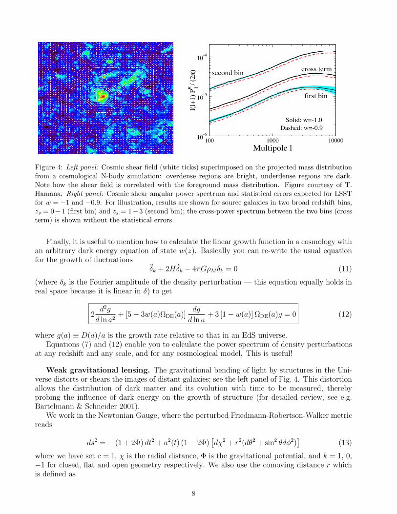
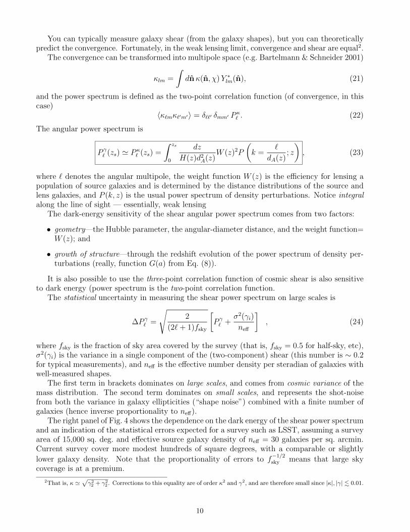
Figure 4: Left panel: Cosmic shear field (white ticks) superimposed on the projected mass distributionfrom a cosmological N-body simulation: overdense regions are bright, underdense regions are dark.Note how the shear field is correlated with the foreground mass distribution. Figure courtesy of T.Hamana. Right panel: Cosmic shear angular power spectrum and statistical errors expected for LSSTfor w = −1 and −0.9. For illustration, results are shown for source galaxies in two broad redshift bins,zs = 0−1 (first bin) and zs = 1−3 (second bin); the cross-power spectrum between the two bins (crossterm) is shown without the statistical errors.

Finally, it is useful to mention how to calculate the linear growth function in a cosmology withan arbitrary dark energy equation of state w(z). Basically you can re-write the usual equationfor the growth of fluctuations

δk + 2Hδk − 4πGρMδk = 0 (11)

(where δk is the Fourier amplitude of the density perturbation — this equation equally holds inreal space because it is linear in δ) to get

2d2g

d ln a2+ [5− 3w(a)ΩDE(a)]

dg

d ln a+ 3 [1− w(a)] ΩDE(a)g = 0 (12)

where g(a) ≡ D(a)/a is the growth rate relative to that in an EdS universe.Equations (7) and (12) enable you to calculate the power spectrum of density perturbations

at any redshift and any scale, and for any cosmological model. This is useful!

Weak gravitational lensing. The gravitational bending of light by structures in the Uni-verse distorts or shears the images of distant galaxies; see the left panel of Fig. 4. This distortionallows the distribution of dark matter and its evolution with time to be measured, therebyprobing the influence of dark energy on the growth of structure (for detailed review, see e.g.Bartelmann & Schneider 2001).

We work in the Newtonian Gauge, where the perturbed Friedmann-Robertson-Walker metricreads

ds2 = − (1 + 2Φ) dt2 + a2(t) (1− 2Φ)[dχ2 + r2(dθ2 + sin2 θdφ2)

](13)

where we have set c = 1, χ is the radial distance, Φ is the gravitational potential, and k = 1, 0,−1 for closed, flat and open geometry respectively. We also use the comoving distance r whichis defined as

8

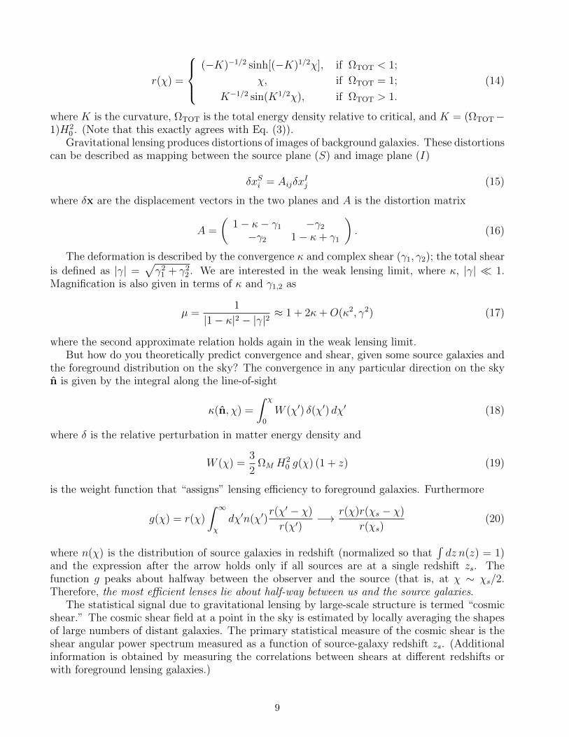
r(χ) =

(−K)−1/2 sinh[(−K)1/2χ], if ΩTOT < 1;

χ, if ΩTOT = 1;

K−1/2 sin(K1/2χ), if ΩTOT > 1.

(14)

where K is the curvature, ΩTOT is the total energy density relative to critical, and K = (ΩTOT−1)H2

0 . (Note that this exactly agrees with Eq. (3)).Gravitational lensing produces distortions of images of background galaxies. These distortions

can be described as mapping between the source plane (S) and image plane (I)

δxSi = AijδxIj (15)

where δx are the displacement vectors in the two planes and A is the distortion matrix

A =

(1− κ− γ1 −γ2

−γ2 1− κ+ γ1

). (16)

The deformation is described by the convergence κ and complex shear (γ1, γ2); the total shear

is defined as |γ| =√γ2

1 + γ22 . We are interested in the weak lensing limit, where κ, |γ| 1.

Magnification is also given in terms of κ and γ1,2 as

µ =1

|1− κ|2 − |γ|2 ≈ 1 + 2κ+O(κ2, γ2) (17)

where the second approximate relation holds again in the weak lensing limit.But how do you theoretically predict convergence and shear, given some source galaxies and

the foreground distribution on the sky? The convergence in any particular direction on the skyn is given by the integral along the line-of-sight

κ(n, χ) =

∫ χ

0

W (χ′) δ(χ′) dχ′ (18)

where δ is the relative perturbation in matter energy density and

W (χ) =3

2ΩM H2

0 g(χ) (1 + z) (19)

is the weight function that “assigns” lensing efficiency to foreground galaxies. Furthermore

g(χ) = r(χ)

∫ ∞

χ

dχ′n(χ′)r(χ′ − χ)

r(χ′)−→ r(χ)r(χs − χ)

r(χs)(20)

where n(χ) is the distribution of source galaxies in redshift (normalized so that∫dz n(z) = 1)

and the expression after the arrow holds only if all sources are at a single redshift zs. Thefunction g peaks about halfway between the observer and the source (that is, at χ ∼ χs/2.Therefore, the most efficient lenses lie about half-way between us and the source galaxies.

The statistical signal due to gravitational lensing by large-scale structure is termed “cosmicshear.” The cosmic shear field at a point in the sky is estimated by locally averaging the shapesof large numbers of distant galaxies. The primary statistical measure of the cosmic shear is theshear angular power spectrum measured as a function of source-galaxy redshift zs. (Additionalinformation is obtained by measuring the correlations between shears at different redshifts orwith foreground lensing galaxies.)

9

You can typically measure galaxy shear (from the galaxy shapes), but you can theoreticallypredict the convergence. Fortunately, in the weak lensing limit, convergence and shear are equal2.

The convergence can be transformed into multipole space (e.g. Bartelmann & Schneider 2001)

κlm =

∫dnκ(n, χ)Y ∗lm(n), (21)

and the power spectrum is defined as the two-point correlation function (of convergence, in thiscase)

〈κ`mκ`′m′〉 = δ``′ δmm′ P κ` . (22)

The angular power spectrum is

P γ` (zs) ' P κ

` (zs) =

∫ zs

0

dz

H(z)d2A(z)

W (z)2P

(k =

`

dA(z); z

), (23)

where ` denotes the angular multipole, the weight function W (z) is the efficiency for lensing apopulation of source galaxies and is determined by the distance distributions of the source andlens galaxies, and P (k, z) is the usual power spectrum of density perturbations. Notice integralalong the line of sight — essentially, weak lensing

The dark-energy sensitivity of the shear angular power spectrum comes from two factors:

• geometry—the Hubble parameter, the angular-diameter distance, and the weight function=W (z); and

• growth of structure—through the redshift evolution of the power spectrum of density per-turbations (really, function G(a) from Eq. (8)).

It is also possible to use the three-point correlation function of cosmic shear is also sensitiveto dark energy (power spectrum is the two-point correlation function.

The statistical uncertainty in measuring the shear power spectrum on large scales is

∆P γ` =

√2

(2`+ 1)fsky

[P γ` +

σ2(γi)

neff

], (24)

where fsky is the fraction of sky area covered by the survey (that is, fsky = 0.5 for half-sky, etc),σ2(γi) is the variance in a single component of the (two-component) shear (this number is ∼ 0.2for typical measurements), and neff is the effective number density per steradian of galaxies withwell-measured shapes.

The first term in brackets dominates on large scales, and comes from cosmic variance of themass distribution. The second term dominates on small scales, and represents the shot-noisefrom both the variance in galaxy ellipticities (“shape noise”) combined with a finite number ofgalaxies (hence inverse proportionality to neff).

The right panel of Fig. 4 shows the dependence on the dark energy of the shear power spectrumand an indication of the statistical errors expected for a survey such as LSST, assuming a surveyarea of 15,000 sq. deg. and effective source galaxy density of neff = 30 galaxies per sq. arcmin.Current survey cover more modest hundreds of square degrees, with a comparable or slightly

lower galaxy density. Note that the proportionality of errors to f−1/2sky means that large sky

coverage is at a premium.

2That is, κ '√γ22 + γ2

2 . Corrections to this equality are of order κ2 and γ2, and are therefore small since |κ|, |γ| . 0.01.

10

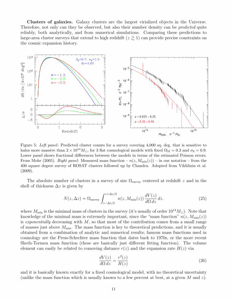
Clusters of galaxies. Galaxy clusters are the largest virialized objects in the Universe.Therefore, not only can they be observed, but also their number density can be predicted quitereliably, both analytically, and from numerical simulations. Comparing these predictions tolarge-area cluster surveys that extend to high redshift (z & 1) can provide precise constraints onthe cosmic expansion history.

z = 0.025 − 0.25

1014 1015

10−9

10−8

10−7

10−6

10−5

M500, h−1

M⊙

N(>

M),

h−

3Mpc

−3

z = 0.35 − 0.90

Figure 5: Left panel: Predicted cluster counts for a survey covering 4,000 sq. deg. that is sensitive tohalos more massive than 2× 1014M, for 3 flat cosmological models with fixed ΩM = 0.3 and σ8 = 0.9.Lower panel shows fractional differences between the models in terms of the estimated Poisson errors.From Mohr (2005). Right panel: Measured mass function – n(z,Mmin(z)) – in our notation – from the400 square degree survey of ROSAT clusters followed up by Chandra. Adopted from Vikhlinin et al.(2009).

The absolute number of clusters in a survey of size Ωsurvey centered at redshift z and in theshell of thickness ∆z is given by

N(z,∆z) = Ωsurvey

∫ z+∆z/2

z−∆z/2

n(z,Mmin(z))dV (z)

dΩ dzdz. (25)

where Mmin is the minimal mass of clusters in the survey (it’s usually of order 1014M). Note thatknowledge of the minimal mass is extremely important, since the “mass function” n(z,Mmin(z))is exponentially decreasing with M , so that most of the contribution comes from a small rangeof masses just above Mmin. The mass function is key to theoretical predictions, and it is usuallyobtained from a combination of analytic and numerical results; famous mass functions used incosmology are the Press-Schechter mass function that dates back to 1970s, or the more recentSheth-Tormen mass function (these are basically just different fitting function). The volumeelement can easily be related to comoving distance r(z) and the expansion rate H(z) via

dV (z)

dΩ dz=r2(z)

H(z)(26)

and it is basically known exactly for a fixed cosmological model, with no theoretical uncertainty(unlike the mass function which is usually known to a few percent at best, at a given M and z).

11

The sensitivity of cluster counts to dark energy arises – as in the case of weak lensing – fromtwo factors:

• geometry, the term dV (z)/(dΩ dz) in Eq. (25) is the comoving volume element

• growth of structure, n(z,Mmin(z)) depends on the evolution of density perturbations, cf.Eq. (11).

This last point is worth emphasizing further. Fitting functions for the cluster mass function(e.g. Press-Schechter) relate it to the primordial spectrum of density perturbations. The massfunction’s near-exponential dependence upon the power spectrum is at the root of the powerof clusters to probe dark energy. In particular, the mass function explicitly depends on theamplitude of mass fluctuations smoothed on some scale R

σ2(R) =

∫ ∞

0

∆2(k)

(3j1(kR)

kR

)2

d ln k (27)

where R is traditionally taken to be ∼ 8 h−1Mpc, the characteristic size of galaxy clusters. Hereof course ∆2(k) is our dear power spectrum from Eq. (7).

Fig. 5 shows the sensitivity to the dark energy equation-of-state parameter of the expectedcluster counts for the South Pole Telescope and the Dark Energy Survey. At modest redshift,z < 0.6, the differences are dominated by the volume element; at higher redshift, the counts aremost sensitive to the growth rate of perturbations.

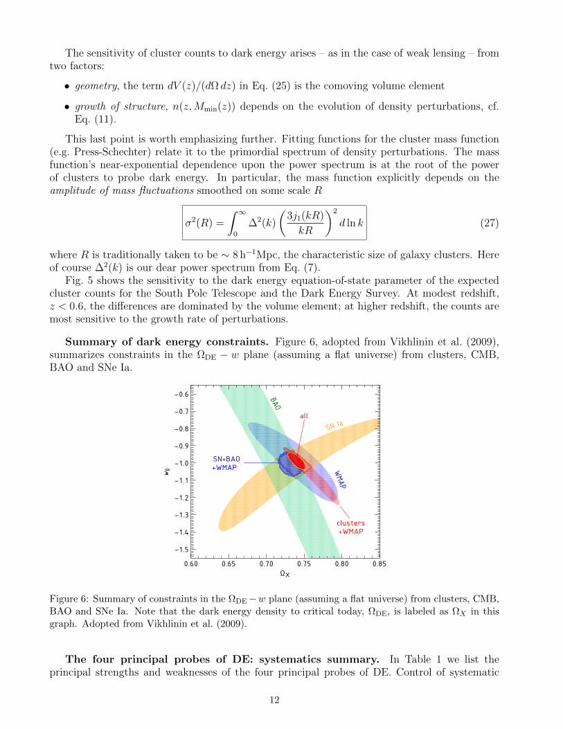
Summary of dark energy constraints. Figure 6, adopted from Vikhlinin et al. (2009),summarizes constraints in the ΩDE − w plane (assuming a flat universe) from clusters, CMB,BAO and SNe Ia.

0.60 0.65 0.70 0.75 0.80 0.85

−1.5−1.4−1.3−1.2−1.1−1.0−0.9−0.8−0.7−0.6

ΩX

w 0

BAO

SN Ia

WMAP

clusters+WMAP

SN+BAO+WMAP

all

Figure 6: Summary of constraints in the ΩDE−w plane (assuming a flat universe) from clusters, CMB,BAO and SNe Ia. Note that the dark energy density to critical today, ΩDE, is labeled as ΩX in thisgraph. Adopted from Vikhlinin et al. (2009).

The four principal probes of DE: systematics summary. In Table 1 we list theprincipal strengths and weaknesses of the four principal probes of DE. Control of systematic

12

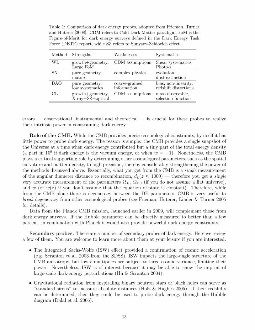
Table 1: Comparison of dark energy probes, adopted from Frieman, Turnerand Huterer [2008]. CDM refers to Cold Dark Matter paradigm, FoM is theFigure-of-Merit for dark energy surveys defined in the Dark Energy TaskForce (DETF) report, while SZ refers to Sunyaev-Zeldovich effect.

Method Strengths Weaknesses Systematics

WL growth+geometry, CDM assumptions Shear systematics,Large FoM Photo-z

SN pure geometry, complex physics evolution,mature dust extinction

BAO pure geometry, coarse-grained bias, non-linearity,low systematics information redshift distortions

CL growth+geometry, CDM assumptions mass-observable,X-ray+SZ+optical selection function

errors — observational, instrumental and theoretical — is crucial for these probes to realizetheir intrinsic power in constraining dark energy.

Role of the CMB. While the CMB provides precise cosmological constraints, by itself it haslittle power to probe dark energy. The reason is simple: the CMB provides a single snapshot ofthe Universe at a time when dark energy contributed but a tiny part of the total energy density(a part in 109 if dark energy is the vacuum energy, or when w = −1). Nonetheless, the CMBplays a critical supporting role by determining other cosmological parameters, such as the spatialcurvature and matter density, to high precision, thereby considerably strengthening the power ofthe methods discussed above. Essentially, what you get from the CMB is a single measurementof the angular diameter distance to recombination, dL(z ≈ 1000) — therefore you get a singlevery accurate measurement of the parameters ΩM , ΩDE (if you do not assume a flat universe),and w (or w(z) if you don’t assume that the equation of state is constant). Therefore, whilefrom the CMB alone there is degeneracy between the DE parameters, CMB is very useful tobreak degeneracy from other cosmological probes (see Frieman, Huterer, Linder & Turner 2005for details).

Data from the Planck CMB mission, launched earlier in 2009, will complement those fromdark energy surveys. If the Hubble parameter can be directly measured to better than a fewpercent, in combination with Planck it would also provide powerful dark energy constraints.

Secondary probes. There are a number of secondary probes of dark energy. Here we reviewa few of them. You are welcome to learn more about them at your leisure if you are interested.

• The Integrated Sachs-Wolfe (ISW) effect provided a confirmation of cosmic acceleration(e.g. Scranton et al. 2003 from the SDSS). ISW impacts the large-angle structure of theCMB anisotropy, but low-` multipoles are subject to large cosmic variance, limiting theirpower. Nevertheless, ISW is of interest because it may be able to show the imprint oflarge-scale dark-energy perturbations (Hu & Scranton 2004).

• Gravitational radiation from inspiraling binary neutron stars or black holes can serve as“standard sirens” to measure absolute distances (Holz & Hughes 2005). If their redshiftscan be determined, then they could be used to probe dark energy through the Hubblediagram (Dalal et al. 2006).

13

• Long-duration gamma-ray bursts have been proposed as standardizable candles (e.g. Schae-fer 2003), but their utility as cosmological distance indicators that could be competitivewith or complementary to SNe Ia has yet to be established. The angular size-redshift re-lation for double radio galaxies has also been used to derive cosmological constraints thatare consistent with dark energy.

• The optical depth for strong gravitational lensing (multiple imaging) of QSOs or radiosources has been proposed and used to provide independent evidence for dark energy,though these measurements depend on modeling the density profiles of lens galaxies.

• The Sandage-Loeb effect (Sandage 1962, Loeb 1998), the redshift change of an objectmeasured using extremely high-resolution spectroscopy over a period of 10 years or more,will some day be useful in constraining the expansion history at higher redshift, 2 . z . 5(Corasaniti, Huterer & Melchiorri 2005).

• Polarization measurements from distant galaxy clusters in principle provide a sensitiveprobe of the growth function and hence dark energy (Cooray, Huterer & Baumann 2004).

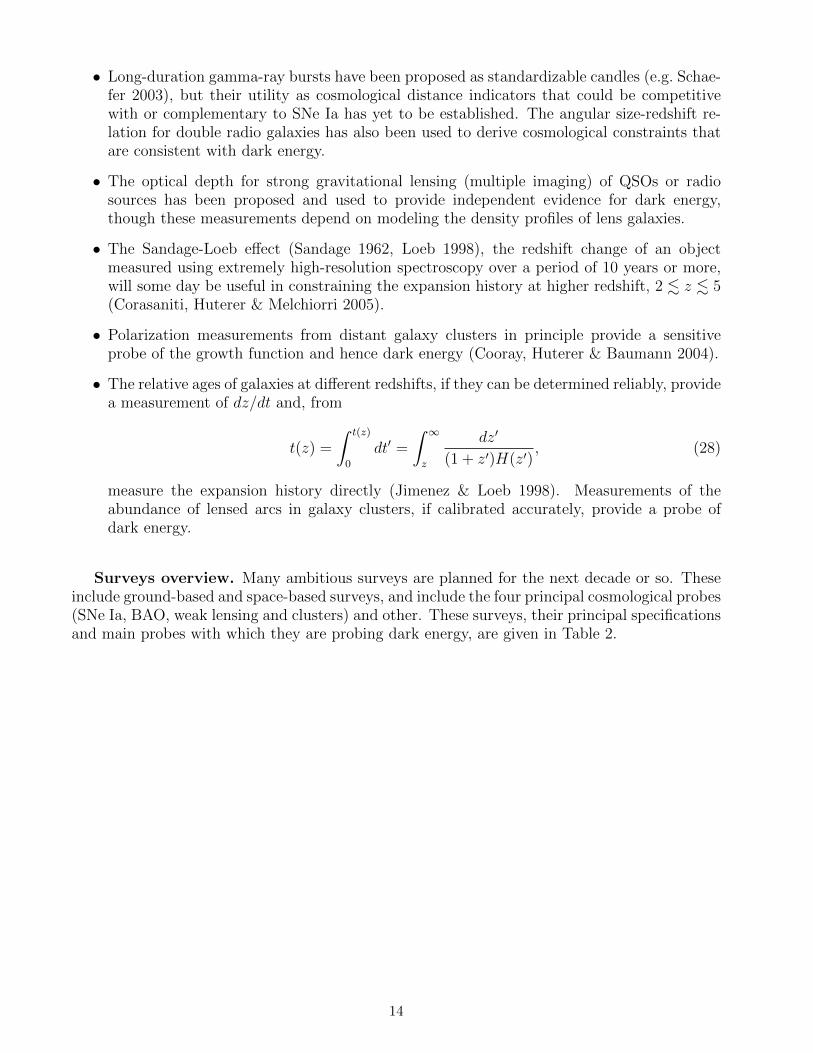
• The relative ages of galaxies at different redshifts, if they can be determined reliably, providea measurement of dz/dt and, from

t(z) =

∫ t(z)

0

dt′ =

∫ ∞

z

dz′

(1 + z′)H(z′), (28)

measure the expansion history directly (Jimenez & Loeb 1998). Measurements of theabundance of lensed arcs in galaxy clusters, if calibrated accurately, provide a probe ofdark energy.

Surveys overview. Many ambitious surveys are planned for the next decade or so. Theseinclude ground-based and space-based surveys, and include the four principal cosmological probes(SNe Ia, BAO, weak lensing and clusters) and other. These surveys, their principal specificationsand main probes with which they are probing dark energy, are given in Table 2.

14

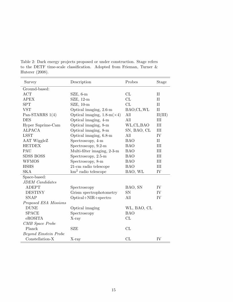
Table 2: Dark energy projects proposed or under construction. Stage refersto the DETF time-scale classification. Adopted from Frieman, Turner &Huterer (2008).

Survey Description Probes Stage

Ground-based:ACT SZE, 6-m CL IIAPEX SZE, 12-m CL IISPT SZE, 10-m CL IIVST Optical imaging, 2.6-m BAO,CL,WL IIPan-STARRS 1(4) Optical imaging, 1.8-m(×4) All II(III)DES Optical imaging, 4-m All IIIHyper Suprime-Cam Optical imaging, 8-m WL,CL,BAO IIIALPACA Optical imaging, 8-m SN, BAO, CL IIILSST Optical imaging, 6.8-m All IVAAT WiggleZ Spectroscopy, 4-m BAO IIHETDEX Spectroscopy, 9.2-m BAO IIIPAU Multi-filter imaging, 2-3-m BAO IIISDSS BOSS Spectroscopy, 2.5-m BAO IIIWFMOS Spectroscopy, 8-m BAO IIIHSHS 21-cm radio telescope BAO IIISKA km2 radio telescope BAO, WL IV

Space-based:JDEM Candidates

ADEPT Spectroscopy BAO, SN IVDESTINY Grism spectrophotometry SN IVSNAP Optical+NIR+spectro All IV

Proposed ESA MissionsDUNE Optical imaging WL, BAO, CLSPACE Spectroscopy BAOeROSITA X-ray CL

CMB Space ProbePlanck SZE CL

Beyond Einstein ProbeConstellation-X X-ray CL IV

15


Topic II: Descriptions of Dark Energy

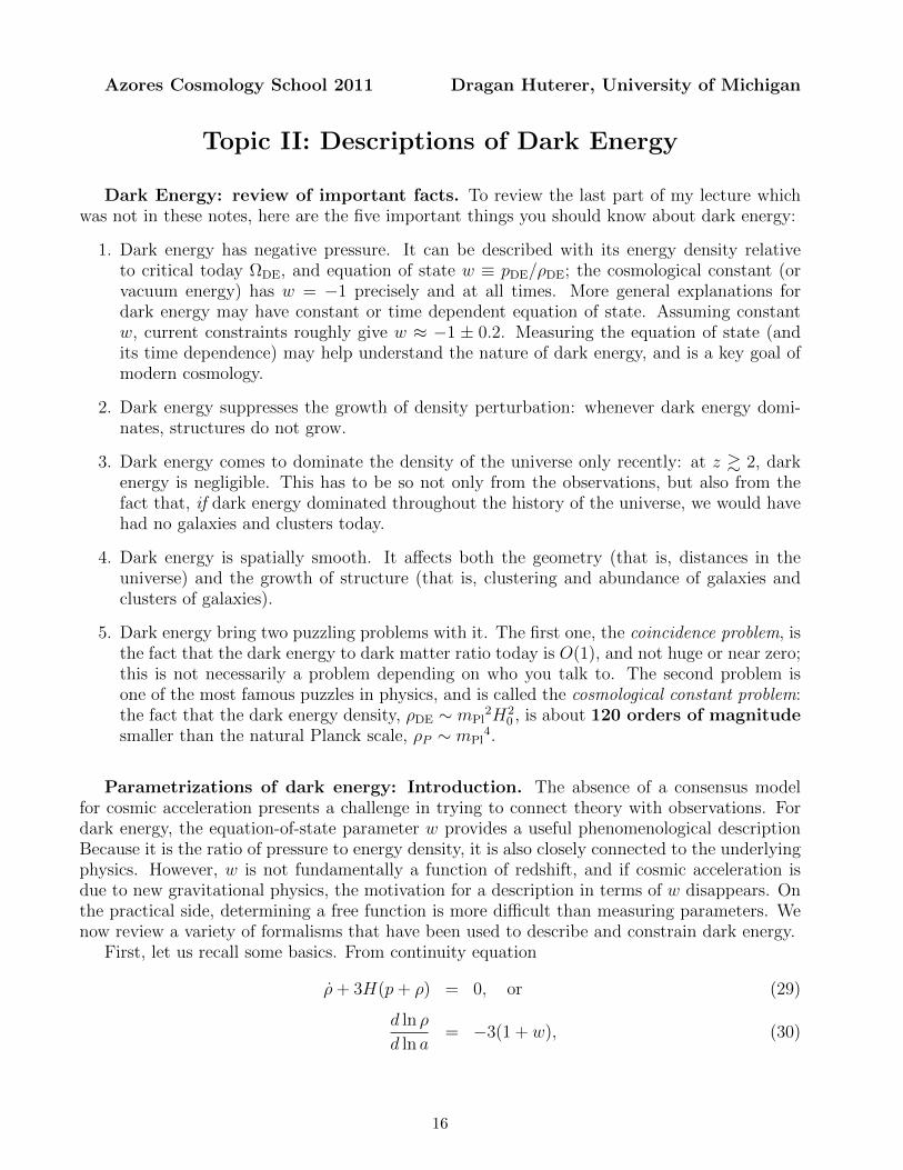
Dark Energy: review of important facts. To review the last part of my lecture whichwas not in these notes, here are the five important things you should know about dark energy:

1. Dark energy has negative pressure. It can be described with its energy density relativeto critical today ΩDE, and equation of state w ≡ pDE/ρDE; the cosmological constant (orvacuum energy) has w = −1 precisely and at all times. More general explanations fordark energy may have constant or time dependent equation of state. Assuming constantw, current constraints roughly give w ≈ −1 ± 0.2. Measuring the equation of state (andits time dependence) may help understand the nature of dark energy, and is a key goal ofmodern cosmology.

2. Dark energy suppresses the growth of density perturbation: whenever dark energy domi-nates, structures do not grow.

3. Dark energy comes to dominate the density of the universe only recently: at z & 2, darkenergy is negligible. This has to be so not only from the observations, but also from thefact that, if dark energy dominated throughout the history of the universe, we would havehad no galaxies and clusters today.

4. Dark energy is spatially smooth. It affects both the geometry (that is, distances in theuniverse) and the growth of structure (that is, clustering and abundance of galaxies andclusters of galaxies).

5. Dark energy bring two puzzling problems with it. The first one, the coincidence problem, isthe fact that the dark energy to dark matter ratio today is O(1), and not huge or near zero;this is not necessarily a problem depending on who you talk to. The second problem isone of the most famous puzzles in physics, and is called the cosmological constant problem:the fact that the dark energy density, ρDE ∼ mPl

2H20 , is about 120 orders of magnitude

smaller than the natural Planck scale, ρP ∼ mPl4.

Parametrizations of dark energy: Introduction. The absence of a consensus modelfor cosmic acceleration presents a challenge in trying to connect theory with observations. Fordark energy, the equation-of-state parameter w provides a useful phenomenological descriptionBecause it is the ratio of pressure to energy density, it is also closely connected to the underlyingphysics. However, w is not fundamentally a function of redshift, and if cosmic acceleration isdue to new gravitational physics, the motivation for a description in terms of w disappears. Onthe practical side, determining a free function is more difficult than measuring parameters. Wenow review a variety of formalisms that have been used to describe and constrain dark energy.

First, let us recall some basics. From continuity equation

ρ+ 3H(p+ ρ) = 0, or (29)

d ln ρ

d ln a= −3(1 + w), (30)

16

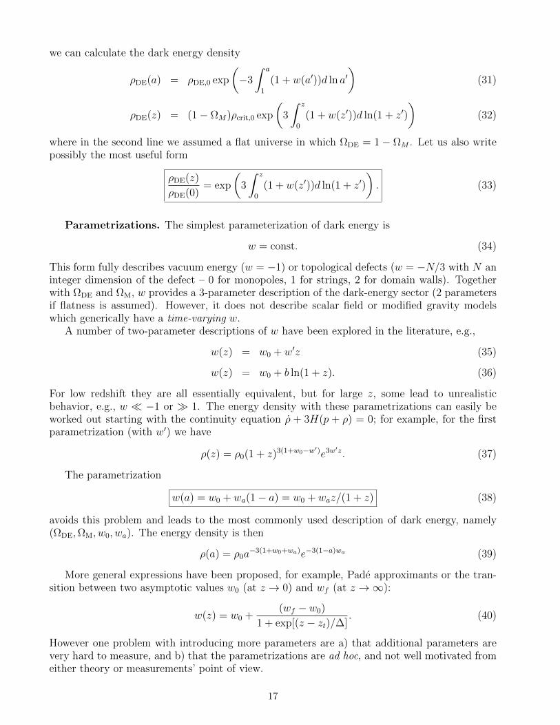
we can calculate the dark energy density

ρDE(a) = ρDE,0 exp

(−3

∫ a

1

(1 + w(a′))d ln a′)

(31)

ρDE(z) = (1− ΩM)ρcrit,0 exp

(3

∫ z

0

(1 + w(z′))d ln(1 + z′)

)(32)

where in the second line we assumed a flat universe in which ΩDE = 1− ΩM . Let us also writepossibly the most useful form

ρDE(z)

ρDE(0)= exp

(3

∫ z

0

(1 + w(z′))d ln(1 + z′)

). (33)

Parametrizations. The simplest parameterization of dark energy is

w = const. (34)

This form fully describes vacuum energy (w = −1) or topological defects (w = −N/3 with N aninteger dimension of the defect – 0 for monopoles, 1 for strings, 2 for domain walls). Togetherwith ΩDE and ΩM, w provides a 3-parameter description of the dark-energy sector (2 parametersif flatness is assumed). However, it does not describe scalar field or modified gravity modelswhich generically have a time-varying w.

A number of two-parameter descriptions of w have been explored in the literature, e.g.,

w(z) = w0 + w′z (35)

w(z) = w0 + b ln(1 + z). (36)

For low redshift they are all essentially equivalent, but for large z, some lead to unrealisticbehavior, e.g., w −1 or 1. The energy density with these parametrizations can easily beworked out starting with the continuity equation ρ + 3H(p + ρ) = 0; for example, for the firstparametrization (with w′) we have

ρ(z) = ρ0(1 + z)3(1+w0−w′)e3w′z. (37)

The parametrization

w(a) = w0 + wa(1− a) = w0 + waz/(1 + z) (38)

avoids this problem and leads to the most commonly used description of dark energy, namely(ΩDE,ΩM, w0, wa). The energy density is then

ρ(a) = ρ0a−3(1+w0+wa)e−3(1−a)wa (39)

More general expressions have been proposed, for example, Pade approximants or the tran-sition between two asymptotic values w0 (at z → 0) and wf (at z →∞):

w(z) = w0 +(wf − w0)

1 + exp[(z − zt)/∆]. (40)

However one problem with introducing more parameters are a) that additional parameters arevery hard to measure, and b) that the parametrizations are ad hoc, and not well motivated fromeither theory or measurements’ point of view.

17

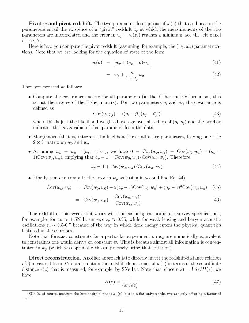
Pivot w and pivot redshift. The two-parameter descriptions of w(z) that are linear in theparameters entail the existence of a “pivot” redshift zp at which the measurements of the twoparameters are uncorrelated and the error in wp ≡ w(zp) reaches a minimum; see the left panelof Fig. 7.

Here is how you compute the pivot redshift (assuming, for example, the (w0, wa) parametriza-tion). Note that we are looking for the equation of state of the form

w(a) = wp + (ap − a)wa (41)

= wp +zp

1 + zpwa (42)

Then you proceed as follows:

• Compute the covariance matrix for all parameters (in the Fisher matrix formalism, thisis just the inverse of the Fisher matrix). For two parameters pi and pj, the covariance isdefined as

Cov(pi, pj) ≡ 〈(pi − pi)(pj − pj)〉 (43)

where this is just the likelihood-weighted average over all values of (pi, pj) and the overbarindicates the mean value of that parameter from the data.

• Marginalize (that is, integrate the likelihood) over all other parameters, leaving only the2× 2 matrix on w0 and wa

• Assuming wp = w0 − (ap − 1)wa, we have 0 = Cov(wp, wa) = Cov(w0, wa) − (ap −1)Cov(wa, wa), implying that ap − 1 = Cov(w0, wa)/Cov(wa, wa). Therefore

ap = 1 + Cov(w0, wa)/Cov(wa, wa) (44)

• Finally, you can compute the error in wp as (using in second line Eq. 44)

Cov(wp, wp) = Cov(w0, w0)− 2(ap − 1)Cov(w0, wa) + (ap − 1)2Cov(wa, wa) (45)

= Cov(w0, w0)− Cov(w0, wa)2

Cov(wa, wa)(46)

The redshift of this sweet spot varies with the cosmological probe and survey specifications;for example, for current SN Ia surveys zp ≈ 0.25, while for weak lensing and baryon acousticoscillations zp ∼ 0.5-0.7 because of the way in which dark energy enters the physical quantitiesfeatured in these probes.

Note that forecast constraints for a particular experiment on wp are numerically equivalentto constraints one would derive on constant w. This is because almost all information is concen-trated in wp (which was optimally chosen precisely using that criterion).

Direct reconstruction. Another approach is to directly invert the redshift-distance relationr(z) measured from SN data to obtain the redshift dependence of w(z) in terms of the coordinatedistance r(z) that is measured, for example, by SNe Ia3. Note that, since r(z) =

∫dz/H(z), we

have

H(z) =1

(dr/dz)(47)

3SNe Ia, of course, measure the luminosity distance dL(z), but in a flat universe the two are only offset by a factor of1 + z.

18

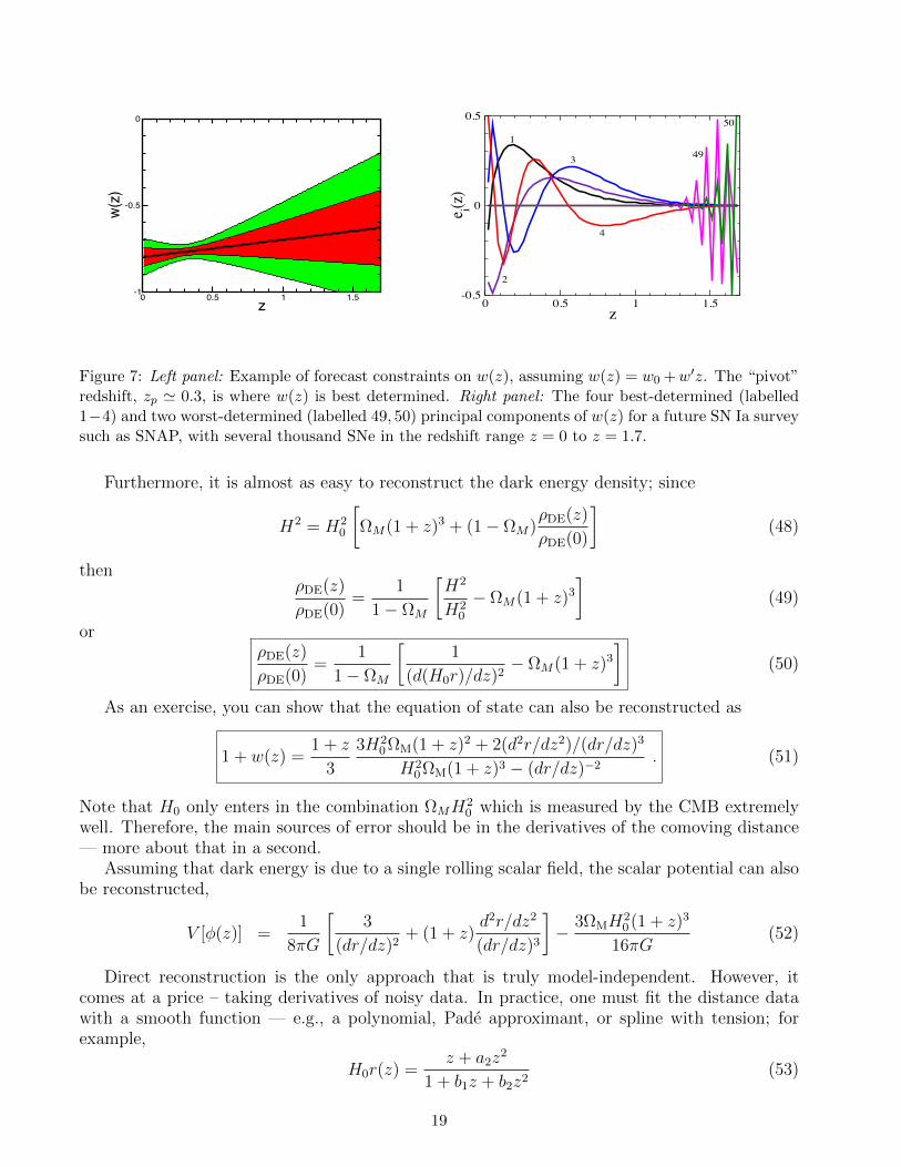
0 0.5 1 1.5z-1

-0.5

0w(z)

0 0.5 1 1.5z

-0.5

0

0.5

e i(z)

1

2

3

4

49

50

Figure 7: Left panel: Example of forecast constraints on w(z), assuming w(z) = w0 +w′z. The “pivot”redshift, zp ' 0.3, is where w(z) is best determined. Right panel: The four best-determined (labelled1−4) and two worst-determined (labelled 49, 50) principal components of w(z) for a future SN Ia surveysuch as SNAP, with several thousand SNe in the redshift range z = 0 to z = 1.7.

Furthermore, it is almost as easy to reconstruct the dark energy density; since

H2 = H20

[ΩM(1 + z)3 + (1− ΩM)

ρDE(z)

ρDE(0)

](48)

thenρDE(z)

ρDE(0)=

1

1− ΩM

[H2

H20

− ΩM(1 + z)3

](49)

orρDE(z)

ρDE(0)=

1

1− ΩM

[1

(d(H0r)/dz)2− ΩM(1 + z)3

](50)

As an exercise, you can show that the equation of state can also be reconstructed as

1 + w(z) =1 + z

3

3H20 ΩM(1 + z)2 + 2(d2r/dz2)/(dr/dz)3

H20 ΩM(1 + z)3 − (dr/dz)−2

. (51)

Note that H0 only enters in the combination ΩMH20 which is measured by the CMB extremely

well. Therefore, the main sources of error should be in the derivatives of the comoving distance— more about that in a second.

Assuming that dark energy is due to a single rolling scalar field, the scalar potential can alsobe reconstructed,

V [φ(z)] =1

8πG

[3

(dr/dz)2+ (1 + z)

d2r/dz2

(dr/dz)3

]− 3ΩMH

20 (1 + z)3

16πG(52)

Direct reconstruction is the only approach that is truly model-independent. However, itcomes at a price – taking derivatives of noisy data. In practice, one must fit the distance datawith a smooth function — e.g., a polynomial, Pade approximant, or spline with tension; forexample,

H0r(z) =z + a2z

2

1 + b1z + b2z2(53)

19

(which is a Pade approximant fit, made so that H0r → z when z 1).The fitting process introduces systematic biases – it is simply very hard to take second

derivative of noisy data (if on a given day you want to be frustrated a little extra, try it!). Whilea variety of methods have been pursued it appears that direct reconstruction is too challengingand not robust even with SN Ia data of excellent quality. Although the expression for ρDE(z)involves only first derivatives of r(z), it contains little information about the nature of darkenergy. For a review of dark energy reconstruction and related issues, see Sahni & Starobinsky2006.

Principal components. The most general, and the only really non-parametric method, toreconstruct properties of DE is that of principal components of dark energy. The cosmologicalfunction that we are trying to determine — w(z), ρDE(z), or H(z) — can be expanded in termsof principal components, a set of functions that are uncorrelated and orthogonal by construction.In this approach, the data determine which aspects of a cosmological function — which linearcombinations of w(zi), in this case — are measured best.

For example, suppose we parametrize w(z) in terms of piecewise constant values wi (i =1, . . . , N), each defined over a small redshift range (zi, zi + ∆z). Then you get the principalcomponents as follows

• Create the covariance matrix of all parameters, including the wi

• Marginalize over all non-w parameters, and be left with the N × N covariance matrix inthe wi — call it C; also compute its inverse, C−1

• Diagonalize the inverse covariance: C−1 = W TΛW , where Λ is diagonal and W is orthog-onal

• Rows of W T are the eigenvectors ei — the “principal components” — while the elementsof Λ give the accuracies in how well each PC is measured. The eigenvectors are of courseorthonormal so that

∫ei(z)ej(z)dz = δij.

In other words

1 + w(z) =N∑

i=1

αi ei(z) , (54)

withσ(αi) = λ

−1/2i (55)

(note that we wisely added unity to w in its expansion, so that the fiducial expansion parametersare zero around ΛCDM).

In the limit of small ∆z this recovers the shape of an arbitrary dark energy history (inpractice, N & 20 is sufficient), but the estimates of the wi from a given dark energy probe willbe very noisy for large N . Principal Component Analysis extracts from those noisy estimatesthe best-measured features of w(z).

The coefficients αi, which can be computed via the orthonormality condition

αi =

∫(1 + w(z))ei(z)dz (56)

Examples of these components are shown for a future SN survey in the right panel of Fig. 7.There are multiple advantages of using the PCs of dark energy (note you can also calculate

PCs of ρDE(z), H(z), etc):

20

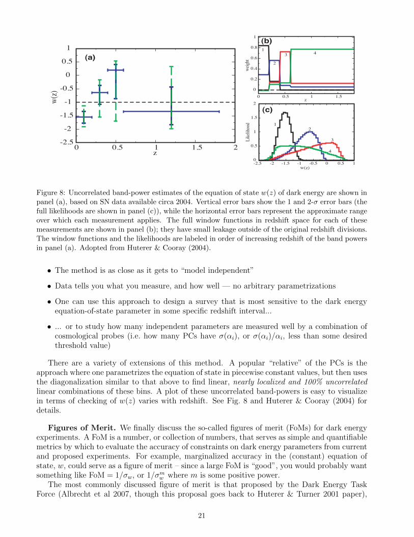
0 0.5 1 1.5 2z

-2.5

-2

-1.5

-1

-0.5

0

0.5

1w(z)

(a)

0 0.5 1 1.5z

0

0.2

0.4

0.6

0.8

1

weight

41

2

3

-2.5 -2 -1.5 -1 -0.5 0 0.5 1w(z)

0

0.5

1

1.5

2

Likelihood 1

2

3

4

(b)

(c)

Figure 8: Uncorrelated band-power estimates of the equation of state w(z) of dark energy are shown inpanel (a), based on SN data available circa 2004. Vertical error bars show the 1 and 2-σ error bars (thefull likelihoods are shown in panel (c)), while the horizontal error bars represent the approximate rangeover which each measurement applies. The full window functions in redshift space for each of thesemeasurements are shown in panel (b); they have small leakage outside of the original redshift divisions.The window functions and the likelihoods are labeled in order of increasing redshift of the band powersin panel (a). Adopted from Huterer & Cooray (2004).

• The method is as close as it gets to “model independent”

• Data tells you what you measure, and how well — no arbitrary parametrizations

• One can use this approach to design a survey that is most sensitive to the dark energyequation-of-state parameter in some specific redshift interval...

• ... or to study how many independent parameters are measured well by a combination ofcosmological probes (i.e. how many PCs have σ(αi), or σ(αi)/αi, less than some desiredthreshold value)

There are a variety of extensions of this method. A popular “relative” of the PCs is theapproach where one parametrizes the equation of state in piecewise constant values, but then usesthe diagonalization similar to that above to find linear, nearly localized and 100% uncorrelatedlinear combinations of these bins. A plot of these uncorrelated band-powers is easy to visualizein terms of checking of w(z) varies with redshift. See Fig. 8 and Huterer & Cooray (2004) fordetails.

Figures of Merit. We finally discuss the so-called figures of merit (FoMs) for dark energyexperiments. A FoM is a number, or collection of numbers, that serves as simple and quantifiablemetrics by which to evaluate the accuracy of constraints on dark energy parameters from currentand proposed experiments. For example, marginalized accuracy in the (constant) equation ofstate, w, could serve as a figure of merit – since a large FoM is “good”, you would probably wantsomething like FoM = 1/σw, or 1/σmw where m is some positive power.

The most commonly discussed figure of merit is that proposed by the Dark Energy TaskForce (Albrecht et al 2007, though this proposal goes back to Huterer & Turner 2001 paper),

21

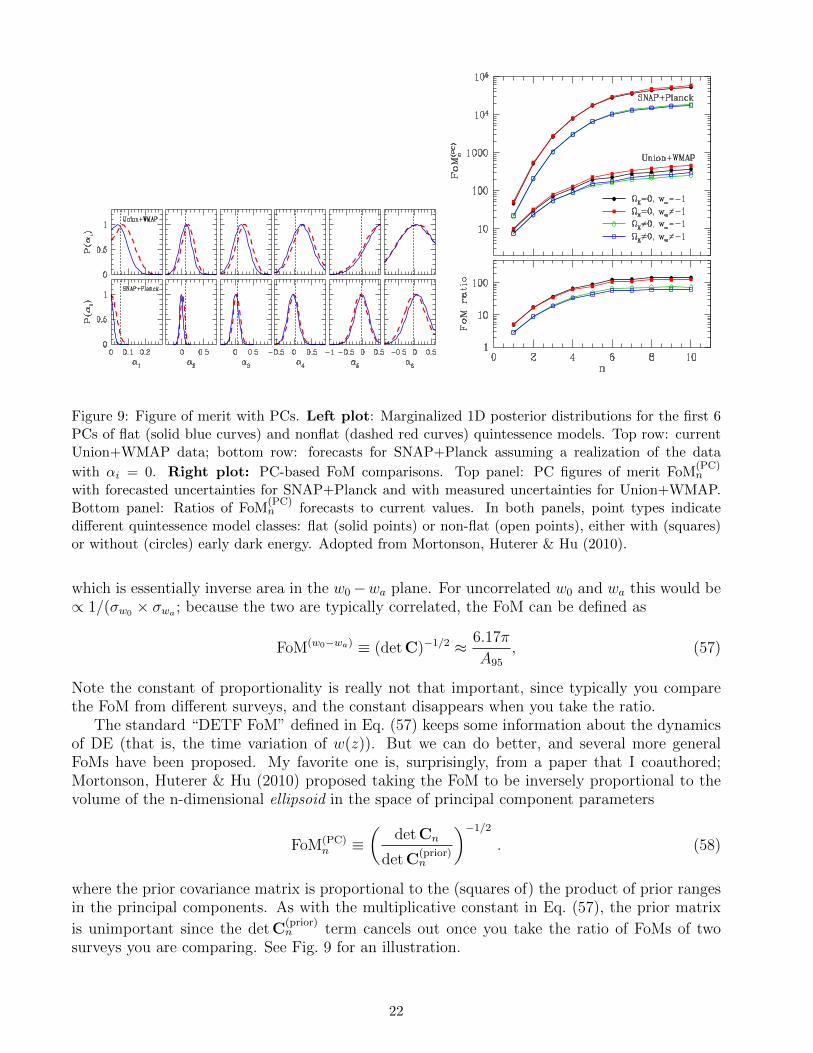
Figure 9: Figure of merit with PCs. Left plot: Marginalized 1D posterior distributions for the first 6PCs of flat (solid blue curves) and nonflat (dashed red curves) quintessence models. Top row: currentUnion+WMAP data; bottom row: forecasts for SNAP+Planck assuming a realization of the data

with αi = 0. Right plot: PC-based FoM comparisons. Top panel: PC figures of merit FoM(PC)n

with forecasted uncertainties for SNAP+Planck and with measured uncertainties for Union+WMAP.Bottom panel: Ratios of FoM

(PC)n forecasts to current values. In both panels, point types indicate

different quintessence model classes: flat (solid points) or non-flat (open points), either with (squares)or without (circles) early dark energy. Adopted from Mortonson, Huterer & Hu (2010).

which is essentially inverse area in the w0−wa plane. For uncorrelated w0 and wa this would be∝ 1/(σw0 × σwa ; because the two are typically correlated, the FoM can be defined as

FoM(w0−wa) ≡ (detC)−1/2 ≈ 6.17π

A95

, (57)

Note the constant of proportionality is really not that important, since typically you comparethe FoM from different surveys, and the constant disappears when you take the ratio.

The standard “DETF FoM” defined in Eq. (57) keeps some information about the dynamicsof DE (that is, the time variation of w(z)). But we can do better, and several more generalFoMs have been proposed. My favorite one is, surprisingly, from a paper that I coauthored;Mortonson, Huterer & Hu (2010) proposed taking the FoM to be inversely proportional to thevolume of the n-dimensional ellipsoid in the space of principal component parameters

FoM(PC)n ≡

(detCn

detC(prior)n

)−1/2

. (58)

where the prior covariance matrix is proportional to the (squares of) the product of prior rangesin the principal components. As with the multiplicative constant in Eq. (57), the prior matrix

is unimportant since the detC(prior)n term cancels out once you take the ratio of FoMs of two

surveys you are comparing. See Fig. 9 for an illustration.

22


Topic III: Cosmological data and likelihood analysis

Recommended reading: There are some excellent resources on topics covered here.

• “Numerical Recipes - the Art of Scientific Computing”, Press, Teukolsky, Vetterling &Flannery — A famous book that doesn’t disappoint on topics of interest here — see itschapter 15.

• “Bayes in the sky: Bayesian inference and model selection in cosmology”, R. Trotta,arXiv:0803.4089 — A fairly complete scripture of various Bayesian techniques from oneof the Apostles.

• “A practical guide to Basic Statistical Techniques for Data Analysis in Cosmology”, L.Verde, arXiv:0712.3028 — A good, broad but rushed overview of various numerical/statisticaltopics in cosmology, with a good list of references.

• “Karhunen-Loeve Eigenvalue Problems in Cosmology: How Should We Tackle Large DataSets?”, M. Tegmark, A. Taylor and A. Heavens, ApJ, 480, 22 (1997) — one of the papersthat introduced the Fisher matrix to cosmology; explained well and major bonus materialson data compression in cosmology if you are interested.

• “Unified approach to the classical statistical analysis of small signals”, G.J. Feldman andR.D. Cousins, PRD, 57, 3873 (1998) — If you would like to be a frequentist, read this veryclear and important paper, which also gives applications to neutrino oscillation data.

Bayesian vs. frequentist. There are two principal approaches to statistics, and theircompetition is as famous as that between the Montagues and Capulets, or the Lakers and theCeltics. These are the Bayesian and frequentist approaches.

Frequentist interpretation of probability defines an event’s probability as the limit of itsrelative frequency in a large number of trials. So I observe the event unfold many times and, inthe limit when that number goes to infinity, the relative frequency of its outcome becomes itsprobability.

Bayesian probability interprets the concept of probability as ’a measure of a state of knowl-edge, and not as a frequency. One of the crucial features of the Bayesian view is that a probabilitycan be assigned to a hypothesis, which is not possible under the frequentist view, where a hy-pothesis can only be rejected or not rejected.

More formally, the Bayesian probability calculus makes use of Bayes’ formula - a theoremthat is valid in all common interpretations of probability - in the following way:

P (M |D) =P (D|M)P (M)

P (D)(Bayes′ theorem) (59)

where M represents a model (or a hypothesis) and D is data. Here

• P (M) is a prior probability of M the probability that M is correct before the data D wasseen

23

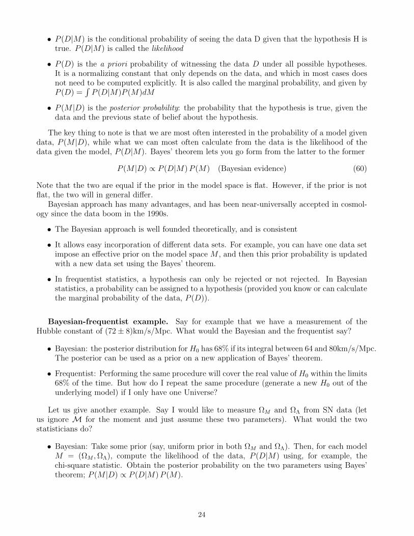
• P (D|M) is the conditional probability of seeing the data D given that the hypothesis H istrue. P (D|M) is called the likelihood

• P (D) is the a priori probability of witnessing the data D under all possible hypotheses.It is a normalizing constant that only depends on the data, and which in most cases doesnot need to be computed explicitly. It is also called the marginal probability, and given byP (D) =

∫P (D|M)P (M)dM

• P (M |D) is the posterior probability: the probability that the hypothesis is true, given thedata and the previous state of belief about the hypothesis.

The key thing to note is that we are most often interested in the probability of a model givendata, P (M |D), while what we can most often calculate from the data is the likelihood of thedata given the model, P (D|M). Bayes’ theorem lets you go form from the latter to the former

P (M |D) ∝ P (D|M)P (M) (Bayesian evidence) (60)

Note that the two are equal if the prior in the model space is flat. However, if the prior is notflat, the two will in general differ.

Bayesian approach has many advantages, and has been near-universally accepted in cosmol-ogy since the data boom in the 1990s.

• The Bayesian approach is well founded theoretically, and is consistent

• It allows easy incorporation of different data sets. For example, you can have one data setimpose an effective prior on the model space M , and then this prior probability is updatedwith a new data set using the Bayes’ theorem.

• In frequentist statistics, a hypothesis can only be rejected or not rejected. In Bayesianstatistics, a probability can be assigned to a hypothesis (provided you know or can calculatethe marginal probability of the data, P (D)).

Bayesian-frequentist example. Say for example that we have a measurement of theHubble constant of (72± 8)km/s/Mpc. What would the Bayesian and the frequentist say?

• Bayesian: the posterior distribution forH0 has 68% if its integral between 64 and 80km/s/Mpc.The posterior can be used as a prior on a new application of Bayes’ theorem.

• Frequentist: Performing the same procedure will cover the real value of H0 within the limits68% of the time. But how do I repeat the same procedure (generate a new H0 out of theunderlying model) if I only have one Universe?

Let us give another example. Say I would like to measure ΩM and ΩΛ from SN data (letus ignore M for the moment and just assume these two parameters). What would the twostatisticians do?

• Bayesian: Take some prior (say, uniform prior in both ΩM and ΩΛ). Then, for each modelM = (ΩM ,ΩΛ), compute the likelihood of the data, P (D|M) using, for example, thechi-square statistic. Obtain the posterior probability on the two parameters using Bayes’theorem; P (M |D) ∝ P (D|M)P (M).

24

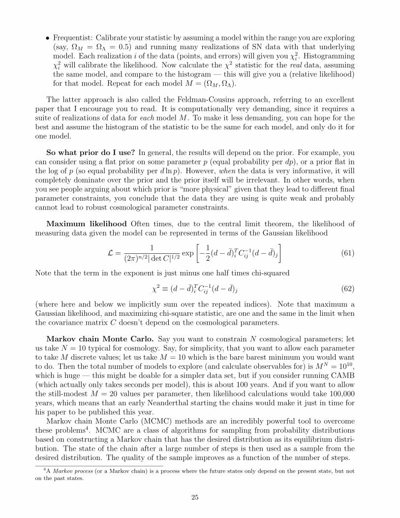
• Frequentist: Calibrate your statistic by assuming a model within the range you are exploring(say, ΩM = ΩΛ = 0.5) and running many realizations of SN data with that underlyingmodel. Each realization i of the data (points, and errors) will given you χ2

i . Histogrammingχ2i will calibrate the likelihood. Now calculate the χ2 statistic for the real data, assuming

the same model, and compare to the histogram — this will give you a (relative likelihood)for that model. Repeat for each model M = (ΩM ,ΩΛ).

The latter approach is also called the Feldman-Cousins approach, referring to an excellentpaper that I encourage you to read. It is computationally very demanding, since it requires asuite of realizations of data for each model M . To make it less demanding, you can hope for thebest and assume the histogram of the statistic to be the same for each model, and only do it forone model.

So what prior do I use? In general, the results will depend on the prior. For example, youcan consider using a flat prior on some parameter p (equal probability per dp), or a prior flat inthe log of p (so equal probability per d ln p). However, when the data is very informative, it willcompletely dominate over the prior and the prior itself will be irrelevant. In other words, whenyou see people arguing about which prior is “more physical” given that they lead to different finalparameter constraints, you conclude that the data they are using is quite weak and probablycannot lead to robust cosmological parameter constraints.

Maximum likelihood Often times, due to the central limit theorem, the likelihood ofmeasuring data given the model can be represented in terms of the Gaussian likelihood

L =1

(2π)n/2| detC|1/2 exp

[−1

2(d− d)Ti C

−1ij (d− d)j

](61)

Note that the term in the exponent is just minus one half times chi-squared

χ2 ≡ (d− d)Ti C−1ij (d− d)j (62)

(where here and below we implicitly sum over the repeated indices). Note that maximum aGaussian likelihood, and maximizing chi-square statistic, are one and the same in the limit whenthe covariance matrix C doesn’t depend on the cosmological parameters.

Markov chain Monte Carlo. Say you want to constrain N cosmological parameters; letus take N = 10 typical for cosmology. Say, for simplicity, that you want to allow each parameterto take M discrete values; let us take M = 10 which is the bare barest minimum you would wantto do. Then the total number of models to explore (and calculate observables for) is MN = 1010,which is huge — this might be doable for a simpler data set, but if you consider running CAMB(which actually only takes seconds per model), this is about 100 years. And if you want to allowthe still-modest M = 20 values per parameter, then likelihood calculations would take 100,000years, which means that an early Neanderthal starting the chains would make it just in time forhis paper to be published this year.

Markov chain Monte Carlo (MCMC) methods are an incredibly powerful tool to overcomethese problems4. MCMC are a class of algorithms for sampling from probability distributionsbased on constructing a Markov chain that has the desired distribution as its equilibrium distri-bution. The state of the chain after a large number of steps is then used as a sample from thedesired distribution. The quality of the sample improves as a function of the number of steps.

4A Markov process (or a Markov chain) is a process where the future states only depend on the present state, but noton the past states.

25

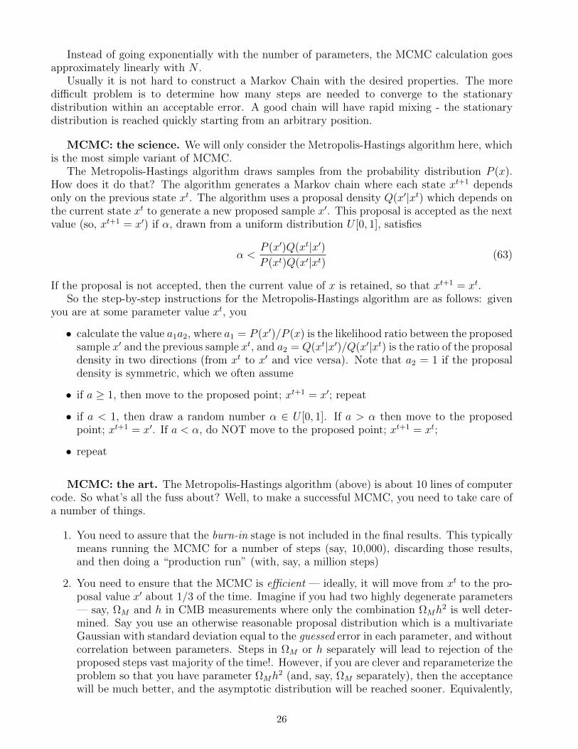
Instead of going exponentially with the number of parameters, the MCMC calculation goesapproximately linearly with N .

Usually it is not hard to construct a Markov Chain with the desired properties. The moredifficult problem is to determine how many steps are needed to converge to the stationarydistribution within an acceptable error. A good chain will have rapid mixing - the stationarydistribution is reached quickly starting from an arbitrary position.

MCMC: the science. We will only consider the Metropolis-Hastings algorithm here, whichis the most simple variant of MCMC.

The Metropolis-Hastings algorithm draws samples from the probability distribution P (x).How does it do that? The algorithm generates a Markov chain where each state xt+1 dependsonly on the previous state xt. The algorithm uses a proposal density Q(x′|xt) which depends onthe current state xt to generate a new proposed sample x′. This proposal is accepted as the nextvalue (so, xt+1 = x′) if α, drawn from a uniform distribution U [0, 1], satisfies

α <P (x′)Q(xt|x′)P (xt)Q(x′|xt) (63)

If the proposal is not accepted, then the current value of x is retained, so that xt+1 = xt.So the step-by-step instructions for the Metropolis-Hastings algorithm are as follows: given

you are at some parameter value xt, you

• calculate the value a1a2, where a1 = P (x′)/P (x) is the likelihood ratio between the proposedsample x′ and the previous sample xt, and a2 = Q(xt|x′)/Q(x′|xt) is the ratio of the proposaldensity in two directions (from xt to x′ and vice versa). Note that a2 = 1 if the proposaldensity is symmetric, which we often assume

• if a ≥ 1, then move to the proposed point; xt+1 = x′; repeat

• if a < 1, then draw a random number α ∈ U [0, 1]. If a > α then move to the proposedpoint; xt+1 = x′. If a < α, do NOT move to the proposed point; xt+1 = xt;

• repeat

MCMC: the art. The Metropolis-Hastings algorithm (above) is about 10 lines of computercode. So what’s all the fuss about? Well, to make a successful MCMC, you need to take care ofa number of things.

1. You need to assure that the burn-in stage is not included in the final results. This typicallymeans running the MCMC for a number of steps (say, 10,000), discarding those results,and then doing a “production run” (with, say, a million steps)

2. You need to ensure that the MCMC is efficient — ideally, it will move from xt to the pro-posal value x′ about 1/3 of the time. Imagine if you had two highly degenerate parameters— say, ΩM and h in CMB measurements where only the combination ΩMh

2 is well deter-mined. Say you use an otherwise reasonable proposal distribution which is a multivariateGaussian with standard deviation equal to the guessed error in each parameter, and withoutcorrelation between parameters. Steps in ΩM or h separately will lead to rejection of theproposed steps vast majority of the time!. However, if you are clever and reparameterize theproblem so that you have parameter ΩMh

2 (and, say, ΩM separately), then the acceptancewill be much better, and the asymptotic distribution will be reached sooner. Equivalently,

26

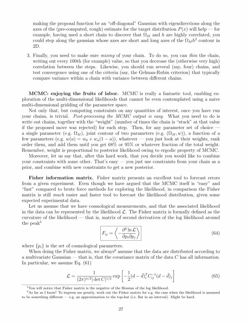
making the proposal function be an “off-diagonal” Gaussian with eigendirections along theaxes of the (pre-computed, rough) estimate for the target distribution P (x) will help — forexample, having used a short chain to discover that ΩM and h are highly correlated, youcould step along the gaussian whose axes are short and long axes of the ΩMh

2 contour in2D.

3. Finally, you need to make sure mixing of your chain. To do so, you can thin the chain,writing out every 100th (for example) value, so that you decrease the (otherwise very high)correlation between the steps. Likewise, you should run several (say, four) chains, andtest convergence using one of the criteria (say, the Gelman-Rubin criterion) that typicallycompare variance within a chain with variance between different chains.

MCMC: enjoying the fruits of labor. MCMC is really a fantastic tool, enabling ex-ploration of the multi-dimensional likelihoods that cannot be even contemplated using a naivemulti-dimensional gridding of the parameter space.

Not only that, but computing constraints on any quantities of interest, once you have runyour chains, is trivial. Post-processing the MCMC output is easy. What you need to do iswrite out chains, together with the “weight” (number of times the chain is “stuck” at that valueif the proposed move was rejected) for each step. Then, for any parameter set of choice —a single parameter (e.g. ΩM), joint contour of two parameters (e.g. (ΩM , w)), a function of afew parameters (e.g. w(a) = w0 + wa(1 − a)), whatever — you just look at their weights, rankorder them, and add them until you get 68% or 95% or whatever fraction of the total weight.Remember, weight is proportional to posterior likelihood owing to ergodic property of MCMC.

Moreover, let us say that, after this hard work, that you decide you would like to combineyour constraints with some other. That’s easy — you just use constraints from your chain as aprior, and combine with new constraints to get a new posterior.

Fisher information matrix. Fisher matrix presents an excellent tool to forecast errorsfrom a given experiment. Even though we have argued that the MCMC itself is “easy” and“fast” compared to brute force methods for exploring the likelihood, in comparison the Fishermatrix is still much easier and faster tool to forecast the likelihood distribution, given someexpected experimental data.

Let us assume that we have cosmological measurements, and that the associated likelihoodin the data can be represented by the likelihood L. The Fisher matrix is formally defined as thecurvature of the likelihood — that is, matrix of second derivatives of the log likelihood aroundthe peak5

Fij =

⟨−∂

2 lnL∂pi∂pj

⟩(64)

where pi is the set of cosmological parameters.When doing the Fisher matrix, we always6 assume that the data are distributed according to

a multivariate Gaussian — that is, that the covariance matrix of the data C has all information.In particular, we assume Eq. (61)

L =1

(2π)n/2| detC|1/2 exp

[−1

2(d− d)Ti C

−1ij (d− d)j

](65)

5You will notice that Fisher matrix is the negative of the Hessian of the log likelihood.6As far as I know! To impress me greatly, work out the Fisher matrix for e.g. the case when the likelihood is assumed

to be something different — e.g. an approximation to the top-hat (i.e. flat in an interval). Might be hard.

27

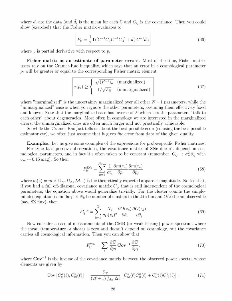
where di are the data (and di is the mean for each i) and Cij is the covariance. Then you couldshow (exercise!) that the Fisher matrix evaluates to

Fij =1

2Tr[C−1C,iC

−1C,j] + dT,i C−1d,j (66)

where ,i is partial derivative with respect to pi.

Fisher matrix as an estimate of parameter errors. Most of the time, Fisher matrixusers rely on the Cramer-Rao inequality, which says that an error in a cosmological parameterpi will be greater or equal to the corresponding Fisher matrix element

σ(pi) ≥

√(F−1)ii (marginalized)

1/√Fii (unmarginalized)

(67)

where ”marginalized” is the uncertainty marginalized over all other N − 1 parameters, while the”unmarginalized” case is when you ignore the other parameters, assuming them effectively fixedand known. Note that the marginalized case has inverse of F which lets the parameters ”talk toeach other” about degeneracies. Most often in cosmology we are interested in the marginalizederrors; the unmarginalized ones are often much larger and not practically achievable.

So while the Cramer-Rao just tells us about the best possible error (so using the best possibleestimator etc), we often just assume that it gives the error from data of the given quality.

Examples. Let us give some examples of the expressions for probe-specific Fisher matrices.For type Ia supernova observations, the covariance matrix of SNe doesn’t depend on cos-

mological parameters, and in fact it’s often taken to be constant (remember, Cij → σ2mδij with

σm ∼ 0.15 mag). So then

F SNeij =

NSNe∑

n=1

1

σ2m

∂m(zn)

∂pi

∂m(zn)

∂pj(68)

where m(z) = m(z,ΩM ,ΩΛ,M...) is the theoretically expected apparent magnitude. Notice that,if you had a full off-diagonal covariance matrix Cij that is still independent of the cosmologicalparameters, the equation above would generalize trivially. For the cluster counts the simple-minded equation is similar; let Nk be number of clusters in the kth bin and O(z) be an observable(say, SZ flux), then

F clusij =

Q∑

k=1

Nk

σO(zk)2

∂O(zk)

∂θi

∂O(zk)

∂θj(69)

Now consider a case of measurements of the CMB (or weak lensing) power spectrum wherethe mean (temperature or shear) is zero and doesn’t depend on cosmology, but the covariancecarries all cosmological information. Then you can show that

FWLij =

∑

`

∂C

∂piCov−1 ∂C

∂pj, (70)

where Cov−1 is the inverse of the covariance matrix between the observed power spectra whoseelements are given by

Cov[Cκij(`), C

κkl(`)

]=

δ``′

(2`+ 1) fsky ∆`

[Cκik(`)C

κjl(`) + Cκ

il(`)Cκjk(`)

]. (71)

28

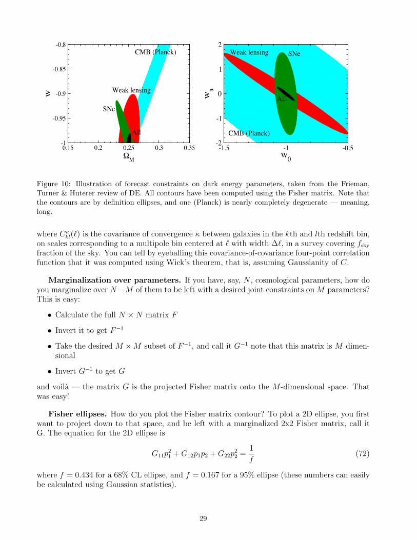
0.15 0.2 0.25 0.3 0.35!M

-1

-0.95

-0.9

-0.85

-0.8w Weak lensing

CMB (Planck)

SNe

All

-1.5 -1 -0.5w0

-2

-1

0

1

2

wa

Weak lensing

CMB (Planck)

SNe

All

Figure 10: Illustration of forecast constraints on dark energy parameters, taken from the Frieman,Turner & Huterer review of DE. All contours have been computed using the Fisher matrix. Note thatthe contours are by definition ellipses, and one (Planck) is nearly completely degenerate — meaning,long.

where Cκkl(`) is the covariance of convergence κ between galaxies in the kth and lth redshift bin,

on scales corresponding to a multipole bin centered at ` with width ∆`, in a survey covering fsky

fraction of the sky. You can tell by eyeballing this covariance-of-covariance four-point correlationfunction that it was computed using Wick’s theorem, that is, assuming Gaussianity of C.

Marginalization over parameters. If you have, say, N , cosmological parameters, how doyou marginalize over N−M of them to be left with a desired joint constraints on M parameters?This is easy:

• Calculate the full N ×N matrix F

• Invert it to get F−1

• Take the desired M ×M subset of F−1, and call it G−1 note that this matrix is M dimen-sional

• Invert G−1 to get G

and voila — the matrix G is the projected Fisher matrix onto the M -dimensional space. Thatwas easy!

Fisher ellipses. How do you plot the Fisher matrix contour? To plot a 2D ellipse, you firstwant to project down to that space, and be left with a marginalized 2x2 Fisher matrix, call itG. The equation for the 2D ellipse is

G11p21 +G12p1p2 +G22p

22 =

1

f(72)

where f = 0.434 for a 68% CL ellipse, and f = 0.167 for a 95% ellipse (these numbers can easilybe calculated using Gaussian statistics).

29

The Fisher ellipse are also show how much information is carried by the data on the pa-rameters — the smaller the ellipse, the more information. More generally, the volume of ann-dimensional ellipsoid is

Volume ∝ (detF )−1/2 . (73)

You can find this useful if you are estimating relative amounts of information in surveys, etc.

Fisher bias. Another great application of the Fisher matrix is to calculate the bias inparameters pi given biases in the observables. This can be derived easily again assuming thesame Gaussian distribution in the data; the result (for weak lensing) is

δpi = F−1ij

∑

`

[Cκα(`)− Cκ

α(`)]

Cov−1[Cκα(`), Cκ

β (`)] ∂Cκ

β (`)

∂pj, (74)

where [Cκα(`), Cκ

β (`)] is the bias in the “observable” shear covariance due to any reason.Perhaps a simpler example would be that for SNeIa, where the bias in the parameters takes

the form

δpi = F−1ij

∑

n

1

σ2m

[m(zn)− m(zn)]∂m(zn)

∂pj(75)

where [m(zn)− m(zn)] is the bias in the observed apparent magnitudes.The bias formula is extremely useful if you would like to see what effect on cosmological

parameter errors an arbitrary systematic effect makes. So, given some biases in the observablequantities, for example [Cκ

α(`) − Cκα(`)] in Eq. (74), you can find biases in the cosmological

parameters δpi. Then you can compare those biases with the statistical errors in the cosmo-logical parameters σ(pi) and impose requirements on the control of your systematic effect sothat |δpi|/σ(pi) is no larger than some threshold, say 0.3 (corresponding to < 30% bias in theparameters). See the paper by Huterer & Takada (2006) for application to how well theoreticalprediction for the power spectrum P (k) needs to be know in order not to “mess up” cosmologicalparameter determinations.

30

Some concepts from Dark Energy and Statistical methods

Documents

Transcript of Some concepts from Dark Energy and Statistical methods