SOLVING LINEAR RATIONAL EXPECTATIONS MODELS

CHRISTOPHER A. SIMS

1. GENERAL FORM OF THE MODELS

The models we are interested in can be cast in the form

Γ0y(t) = Γ1y(t−1)+C+Ψz(t)+Πη(t) (1)

t = 1, . . . ,T, whereC is a vector of constants,z(t) is an exogenously evolving, possi-bly serially correlated, random disturbance, andη(t) is an expectational error, satisfyingEtη(t +1) = 0, all t. Theη(t) terms are not given exogenously, but instead are treated asdetermined as part of the model solution. Models with more lags, or with lagged expec-tations, or with expectations of more distant future values, can be accommodated in thisframework by expanding the y vector. This paper’s analysis is similar to that ofBlanchardand Kahn(1980) with four important differences:

(i) They assume regularity conditions as they proceed that leave some models encoun-tered in practice outside the range of their analysis, while this paper covers all linearmodels with expectational error terms.

(ii) They require that the analyst specify which elements of the y vector are prede-termined, while this paper recognizes that the structure of theΓ0, Γ1, Ψ, andΠmatrices fixes the list of predetermined variables. Our approach therefore handlesautomatically situations where linear combinations of variables, not individual vari-ables, are predetermined.

(iii) This paper makes an explicit extension to continuous time, which raises some dis-tinct analytic difficulties.

(iv) They assume that boundary conditions at infinity are given in the form of a maximalrate of growth for any element of they vector, whereas this paper recognizes thatin general only certain linear combinations of variables are required to grow at

Date: August 1995. Revised February 1996, September 1997, January 2000.This paper has benefited from so many comments from so many people over its overlong gestation that

I cannot list everyone. Particularly important were Jinill Kim, Gary Anderson, and an anonymous referee.c©1995, 1996, 1997, 2000 by Christopher A. Sims. This material may be reproduced for educational andresearch purposes so long as the copies are not sold, even to recover costs, the document is not altered, andthis copyright notice is included in the copies.

1

LINEAR RE MODELS 2

bounded rates and that different linear combinations may have different growthrate restrictions.

There are other more recent papers dealing with models like these (King and Watson,1997, 1998; Anderson, 1997; Klein, 1997) that, like this one, expand the range of modelscovered beyond what is covered in Blanchard and Kahn’s paper, particularly to includesingularΓ0 cases. All these papers, though, follow Blanchard and Kahn in requiring thespecification of “jump" and “predetermined"variables, rather than recognizing that in equi-librium models expectational residuals more naturally are attached to equations. Also, onlyAnderson(1997) has discussed the continuous time case.

Less fundamentally, this paper uses a notation in which time arguments or subscriptsrelate consistently to the information structure: variables datedt are always known att.Blanchard and Kahn’s use of a different convention often leads to confusion in the applica-tion of their method to complex models.

An instructive example to illustrate how we get a model into the form(1) is a model ofoverlapping contracts in wage setting along the lines laid out by Taylor.

w(t) = 13Et [W(t)+W(t +1)+W(t +2)]−α(u(t)−un)+ν(t)

W(t) = 13 (w(t)+w(t−1)+w(t−2))

u(t) = θu(t−1)+ γW(t)+ µ + ε(t) ,

(2)

whereEtν(t +1) = Etε(t +1) = 0. To cast(2) into the form (1) requires using the expandedstate vector

y(t) =

w(t)w(t−1)

W(t)u(t)

EtW(t +1)

(3)

LINEAR RE MODELS 3

With this definition ofy, (2) can be written in the matrix notation of(1), with definitionalequations added, by defining

Γ0 =

0 0 13 0 1

3−1

3 −13 1 0 0

0 0 −γ 1 00 1 0 0 00 0 1 0 0

, Γ1 =

1 0 −13 α 0

0 13 0 0 0

0 0 0 0 θ 01 0 0 0 00 0 0 0 1

,

C =

α ·un

0µ00

, Ψ =

1 00 00 10 00 0

, Π =

0 10 00 00 01 0

,

z(t) =[

ε(t)ν(t−1)

].

(4)

This example illustrates the principle that we can always get a linear model into theform (1) by replacing terms of the formEtx(t +1) with y(t) = Etx(t + 1) and adding tothe system an equation readingx(t) = y(t−1)+ η(t). When terms of the formEtx(t +s)appear, we simply make a sequence of such variable and equation creations. It is oftenpossible to reach the form(1) with fewer new variables by replacing expectations of vari-ables in equations with actual values of the same variables, while addingη(t) disturbanceterms to the equation. While this approach always produces valid equations, it may lose in-formation contained in the original system and thereby imply spurious indeterminacy. Thedanger arises only in situations where a single equation involves some variables of the formEtX(t +1) and other variables of the formY(t +1). In this case, dropping theEt operatorsfrom the equation and adding anη(t) error term loses the information that some variablesare entering as actual values and others as expectations.

The formulation that most writers on this subject have used, following Blanchard andKahn, is

Γ0Ety(t +1) = Γ1y(t)+C+Ψz(t) . (5)

One then adds conditions that certain variables in they vector are “predetermined", mean-ing that for themEty(t +1) = y(t +1). The formulation adopted here embodies the usefulnotational convention, that all variables datedt are observable att; thus no separate list ofwhat is predetermined is needed to augment the information that can be read off from theequations themselves. It also allows straightforward handling of the commonly occurringsystems in which a variableyi(t) and its expectationEt−1yi(t) both appear, with the sametargument, in the same or different equations. To get such systems into the Blanchard-Kahn

LINEAR RE MODELS 4

form requires introducing an extended state vector. For example, in our simple overlappingcontract model(2) above, the fact thatW appears as an expected value in the first equationand/or in the dummy equation defining the artificial state variableζ (t) = EtW(t + 1) (thebottom row of(4)), yet also in two other dynamic equations without any expectation, seemsto require that, to cast the model into standard Blanchard-Quah form, we addw(t−2) andu(t−1) to the list of variables, with two corresponding additional dummy equations.

Standard difference equations of the form(1) have a single, exogenous disturbance vec-tor. That is, they haveΓ0 = I andΠ = 0. They can therefore be interpreted as determiningy(t) for t > t0 from given initial conditionsy(t0) and random draws forz(t). In (1), how-ever, the disturbance vectorΨz(t)+Πη(t) defined in (1) is not exogenously given the wayz(t) itself is. Instead, it depends ony(t) and its expectation, both of which are generallyunknown before we solve the model. Because we need to determineη(t) from z(t) as wesolve the model, we generally need to find a number of additional equations or restrictionsequal to the rank of the matrix in order to obtain a solution.

2. CANONICAL FORMS AND MATRIX DECOMPOSITIONS

Solving a system like(1) subject to restrictions on the rates of growth of components ofits solutions requires breaking its solutions into components with distinct rates of growth.This is best done with some version of an eigenvalue-eigenvector decomposition. We arealready imposing a somewhat stringent canonical form on the equation system by insistingthat it involve just one lag and just one-step-ahead expectations. Of course as we made clearin the example above, systems with more lags or with multi-step and lagged expectationscan be transformed into systems of the form given here, but there may be some computa-tional work in making the transformation. Further tradeoffs between system simplicity andsimplicity of the solution process are possible.

To illustrate this point, we begin by assuming a very stringent canonical form for thesystem:Γ0 = I , Etz(t +1) = 0, all t. Systems derived from even moderately large rationalexpectation equilibrium models often have singularΓ0 matrices, so that simply “multiply-ing through byΓ−1

0 " to achieve this canonical form is not possible. In most economicmodels, there is little guidance available from theory in specifying properties forz. Therequirement thatEtz(t +1) = 0 is therefore extremely restrictive.

On the other hand, it is usually possible, by solving for some variables in terms of othersand thereby reducing system size, to manipulate the system into a form with non-singularΓ0. And it is common practice to make a model tractable by assuming a simple flexibleparametric form for the process generating exogenous variables, so that the exogenous vari-ables themselves are incorporated into they vector, while the serially uncorrelatedzvectorin the canonical form is just the disturbance vector in the process generating the exogenousvariables. So this initial very simple canonical form is in some sense not restrictive.

LINEAR RE MODELS 5

Nonetheless, getting the system into a form with non-singularΓ0 may involve very sub-stantial computational work if it is done ad hoc, on an even moderately large system. Andit is often useful to display the dependence ofy on current, past, and expected future exoge-nous variables directly, rather than to make precise assumptions on how expected futurez’sdepend on current and pastz’s. For these reasons, we will below display solution methodsthat work on more general canonical forms. While these more general solution methodsare themselves harder to understand, they shift the burden of analysis from the individualeconomist/model-solver toward the computer, and are therefore useful.

3. USING THE JORDAN DECOMPOSITION WITH SERIALLY UNCORRELATED SHOCKS

3.1. Discrete time. In this section we consider the special case of

y(t) = Γ1y(t−1)+C+Ψz(t)+Πη(t) , (6)

with Etz(t +1) = 0. The system matrixΓ1 has a Jordan decomposition

Γ1 = PΛP−1 , (7)

whereP is the matrix of right-eigenvectors ofΓ1, P−1 is the matrix of left-eigenvectors,and Λ has the eigenvalues ofΓ1 on its main diagonal and 0’s everywhere else, exceptthat it may haveλi,i+1 = 1 in positions where the corresponding diagonal elements satisfyλii = λi+1,i+1. Multiplying the system on the left byP−1, and definingw= P−1y, we arriveat

w(t) = Λw(t−1)+P−1C+P−1 · (Ψz(t)+Πη(t)) . (8)

In this setting, we can easily consider non-homogeneous growth rate restrictions. That is,suppose that we believe that a set of linear combinations of variables,φiy(t), i = 1, . . . ,m,have bounded growth rates, with possibly different bounding growth rates for eachi. Thatis we believe that a solution must satisfy

Es[φiy(t)ξ−t

i

] →t→∞

0 (9)

for eachi ands, with ξi > 1 for everyi. Equation (8) has isolated components of the systemthat grow at distinct exponential rates. The matrix has a block- diagonal structure, so thatthe system breaks into unrelated components, with a typical block having the form

w j (t) =

λ j 1 0 · · · 0

0 λ j 1...

...

0 0... ... 0

...... . .. λ j 1

0 · · · 0 0 λ j

w j (t−1)+P j·C+P j· · (Ψz(t)+Πη(t)) , (10)

LINEAR RE MODELS 6

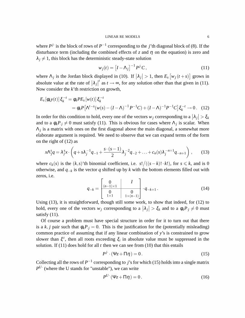
whereP j· is the block of rows ofP−1 corresponding to thej ’th diagonal block of (8). If thedisturbance term (including the combined effects ofz andη on the equation) is zero andλ j 6= 1, this block has the deterministic steady-state solution

w j(t) =[I −Λ j

]−1P j·C , (11)

whereΛ j is the Jordan block displayed in(10). If∣∣λ j

∣∣ > 1, thenEs[w j (t +s)

]grows in

absolute value at the rate of∣∣λ j

∣∣t ast → ∞, for any solution other than that given in(11).Now consider thek’th restriction on growth,

Es[φky(t)]ξ−tk = φkPEs[w(t)]ξ−t

k

= φkP[Λt−s(w(s)− (I −Λ)−1P−1C)+(I −Λ)−1P−1C

]ξ−t

k → 0. (12)

In order for this condition to hold, every one of the vectorsw j corresponding to a∣∣λ j

∣∣ > ξk

and to aφkP· j 6= 0 must satisfy(11). This is obvious for cases whereΛ j is scalar. WhenΛ j is a matrix with ones on the first diagonal above the main diagonal, a somewhat moreelaborate argument is required. We need to observe that we can expand terms of the formon the right of(12) as

xΛsjq = λ s

j x ·(

q+sλ−1j q−1 +

s· (s−1)2

λ−2j q−2 + . . .+cn(s)λ−n+1

j q−n+1

), (13)

whereck(s) is the(k,s)’th binomial coefficient, i.e.s!/((s−k)! ·k!), for s 6 k, and is 0

otherwise, andq−k is the vectorq shifted up byk with the bottom elements filled out withzeros, i.e.

q−k =

0(n−1)×1

I

01×1

01×(n−1)

·q−k+1 . (14)

Using (13), it is straightforward, though still some work, to show that indeed, for(12) tohold, every one of the vectorsw j corresponding to a

∣∣λ j∣∣ > ξk and to aφkP· j 6= 0 must

satisfy(11).Of course a problem must have special structure in order for it to turn out that there

is a k, j pair such thatφkP· j = 0. This is the justification for the (potentially misleading)common practice of assuming that if any linear combination ofy’s is constrained to growslower thanξ t , then all roots exceedingξi in absolute value must be suppressed in thesolution. If (11) does hold for allt then we can see from (10) that this entails

P j· · (Ψz+Πη) = 0. (15)

Collecting all the rows ofP−1 corresponding toj ’s for which(15) holds into a single matrixPU · (where the U stands for "unstable"), we can write

PU · (Ψz+Πη) = 0. (16)

LINEAR RE MODELS 7

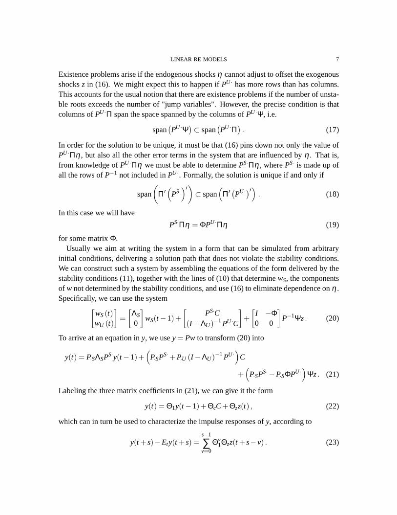
Existence problems arise if the endogenous shocksη cannot adjust to offset the exogenousshocksz in (16). We might expect this to happen ifPU · has more rows than has columns.This accounts for the usual notion that there are existence problems if the number of unsta-ble roots exceeds the number of "jump variables". However, the precise condition is thatcolumns ofPU ·Π span the space spanned by the columns ofPU ·Ψ, i.e.

span(PU ·Ψ

)⊂ span(PU ·Π

). (17)

In order for the solution to be unique, it must be that(16) pins down not only the value ofPU ·Πη , but also all the other error terms in the system that are influenced byη . That is,from knowledge ofPU ·Πη we must be able to determinePS·Πη , wherePS· is made up ofall the rows ofP−1 not included inPU ·. Formally, the solution is unique if and only if

span

(Π′

(PS·

)′)⊂ span

(Π′ (PU ·)′) . (18)

In this case we will have

PS·Πη = ΦPU ·Πη (19)

for some matrixΦ.Usually we aim at writing the system in a form that can be simulated from arbitrary

initial conditions, delivering a solution path that does not violate the stability conditions.We can construct such a system by assembling the equations of the form delivered by thestability conditions(11), together with the lines of (10) that determinewS, the componentsof w not determined by the stability conditions, and use(16) to eliminate dependence onη .Specifically, we can use the system

[wS(t)wU (t)

]=

[ΛS

0

]wS(t−1)+

[PS·C

(I −ΛU)−1PU ·C

]+

[I −Φ0 0

]P−1Ψz. (20)

To arrive at an equation iny, we usey = Pw to transform(20) into

y(t) = P·SΛSPS·y(t−1)+(

P·SPS·+P·U (I −ΛU)−1PU ·)

C

+(

P·SPS·−P·SΦPU ·)

Ψz. (21)

Labeling the three matrix coefficients in(21), we can give it the form

y(t) = Θ1y(t−1)+ΘcC+Θzz(t) , (22)

which can in turn be used to characterize the impulse responses ofy, according to

y(t +s)−Ety(t +s) =s−1

∑v=0

Θv1Θzz(t +s−v) . (23)

LINEAR RE MODELS 8

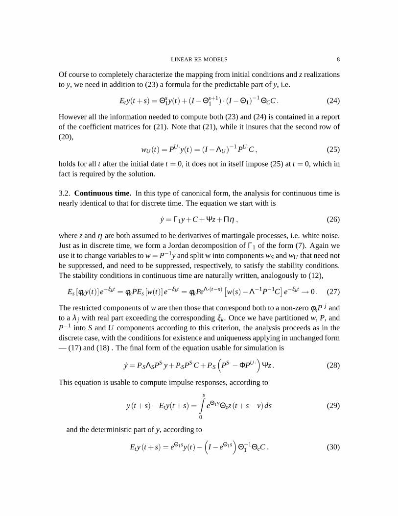
Of course to completely characterize the mapping from initial conditions andz realizationsto y, we need in addition to (23) a formula for the predictable part ofy, i.e.

Ety(t +s) = Θs1y(t)+(I −Θs+1

1 ) · (I −Θ1)−1ΘCC . (24)

However all the information needed to compute both(23) and (24) is contained in a reportof the coefficient matrices for(21). Note that(21), while it insures that the second row of(20),

wU(t) = PU ·y(t) = (I −ΛU)−1PU ·C , (25)

holds for allt after the initial datet = 0, it does not in itself impose(25) at t = 0, which infact is required by the solution.

3.2. Continuous time. In this type of canonical form, the analysis for continuous time isnearly identical to that for discrete time. The equation we start with is

y = Γ1y+C+Ψz+Πη , (26)

wherezandη are both assumed to be derivatives of martingale processes, i.e. white noise.Just as in discrete time, we form a Jordan decomposition ofΓ1 of the form(7). Again weuse it to change variables tow= P−1y and split w into componentswS andwU that need notbe suppressed, and need to be suppressed, respectively, to satisfy the stability conditions.The stability conditions in continuous time are naturally written, analogously to(12),

Es[φky(t)]e−ξkt = φkPEs[w(t)]e−ξkt = φkPeΛ·(t−s) [w(s)−Λ−1P−1C]e−ξkt → 0. (27)

The restricted components ofw are then those that correspond both to a non-zeroφkP· j andto aλ j with real part exceeding the correspondingξk. Once we have partitionedw, P, andP−1 into S andU components according to this criterion, the analysis proceeds as in thediscrete case, with the conditions for existence and uniqueness applying in unchanged form— (17) and (18) . The final form of the equation usable for simulation is

y = P·SΛSPS·y+P·SPS·C+P·S(

PS·−ΦPU ·)

Ψz. (28)

This equation is usable to compute impulse responses, according to

y(t +s)−Ety(t +s) =s∫

0

eΘ1vΘzz(t +s−v)ds (29)

and the deterministic part ofy, according to

Ety(t +s) = eΘ1sy(t)−(

I −eΘ1s)

Θ−11 ΘcC . (30)

LINEAR RE MODELS 9

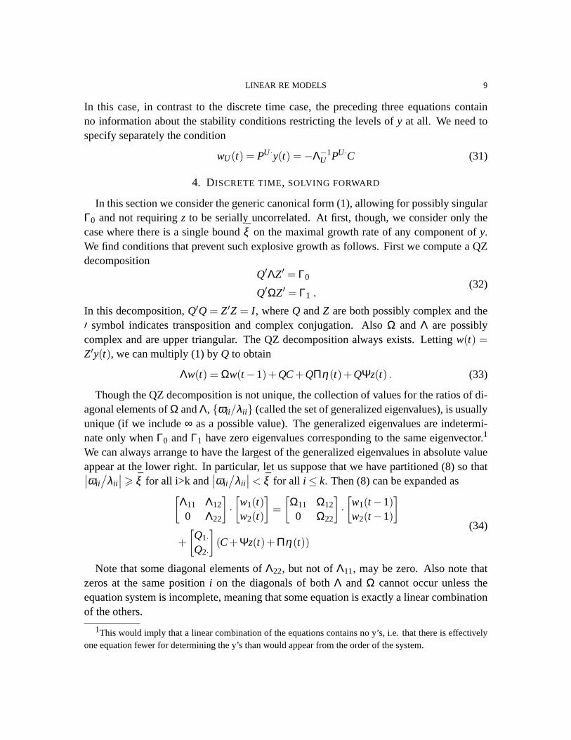
In this case, in contrast to the discrete time case, the preceding three equations containno information about the stability conditions restricting the levels ofy at all. We need tospecify separately the condition

wU(t) = PU ·y(t) =−Λ−1U PU ·C (31)

4. DISCRETE TIME, SOLVING FORWARD

In this section we consider the generic canonical form(1), allowing for possibly singularΓ0 and not requiringz to be serially uncorrelated. At first, though, we consider only thecase where there is a single boundξ on the maximal growth rate of any component ofy.We find conditions that prevent such explosive growth as follows. First we compute a QZdecomposition

Q′ΛZ′ = Γ0

Q′ΩZ′ = Γ1 .(32)

In this decomposition,Q′Q = Z′Z = I , whereQ andZ are both possibly complex and the′ symbol indicates transposition and complex conjugation. AlsoΩ and Λ are possiblycomplex and are upper triangular. The QZ decomposition always exists. Lettingw(t) =Z′y(t), we can multiply(1) by Q to obtain

Λw(t) = Ωw(t−1)+QC+QΠη(t)+QΨz(t) . (33)

Though the QZ decomposition is not unique, the collection of values for the ratios of di-agonal elements ofΩ andΛ, ωii/λii (called the set of generalized eigenvalues), is usuallyunique (if we include∞ as a possible value). The generalized eigenvalues are indetermi-nate only whenΓ0 andΓ1 have zero eigenvalues corresponding to the same eigenvector.1

We can always arrange to have the largest of the generalized eigenvalues in absolute valueappear at the lower right. In particular, let us suppose that we have partitioned(8) so that∣∣ωii

/λii

∣∣ > ξ for all i>k and∣∣ωii

/λii

∣∣ < ξ for all i ≤ k. Then (8) can be expanded as[

Λ11 Λ12

0 Λ22

]·[w1(t)w2(t)

]=

[Ω11 Ω12

0 Ω22

]·[w1(t−1)w2(t−1)

]

+[Q1·Q2·

](C+Ψz(t)+Πη(t))

(34)

Note that some diagonal elements ofΛ22, but not ofΛ11, may be zero. Also note thatzeros at the same positioni on the diagonals of bothΛ and Ω cannot occur unless theequation system is incomplete, meaning that some equation is exactly a linear combinationof the others.

1This would imply that a linear combination of the equations contains no y’s, i.e. that there is effectivelyone equation fewer for determining the y’s than would appear from the order of the system.

LINEAR RE MODELS 10

Because of the way we have grouped the generalized eigenvalues, the lower block ofequations in(33) is purely explosive. It has a solution that does not explode any faster thanthe disturbanceszso long as we solve it "forward" to makew2 a function of future z’s. Thatis, if we label the last additive term in(34) x(t) and setM = Ω−1

22 ·Λ22,

Z′·2y(t) = w2(t) = Mw2(t +1)−Ω−122 x2(t +1)

= M2 ·w2(t +2)−M ·Ω−122 ·x2(t +2)−Ω−1

22 ·x2(t +1)

=−∞

∑s=1

Ms−1 ·Ω−122 ·x2(t +s) . (35)

The last equality in(35) follows on the assumption thatMtw2(t) → 0 ast → ∞. Notethat in the special case ofλii = 0 there are equations in(34) containing no current valuesof w. While these cases do not imply explosive growth, the corresponding components of(35) are still valid. For example, if the lower right element ofΛ is zero, the last equation of(34) has the form

0·wn(t) = ωnn ·wn(t−1)+xn(t). (36)

Solving for wn(t−1) produces the corresponding component of(35). Sinceλii = 0 cor-responds to a singularity inΓ0, the method we are describing handles such singularitiestransparently.

Note that(35) asserts the equality of something on the left that is known at timet tosomething on the right that is a combination of variables datedt +1 and later. Since takingexpectations as of datet leaves the left-hand side unchanged, we can write

Z′·2y(t) = w2(t) =−Et

[∞

∑s=1

Ms−1 ·Ω−122 ·x2(t +s)

]

=−∞

∑s=1

Ms−1 ·Ω−122 ·x2(t +s) . (37)

If the original system(1) consisted of first order conditions from an optimization problem,(37) will be what is usually called the decision rule for the problem. When the originalsystem described a dynamic market equilibrium,(37) will be composed of decision rulesof the various types of agents in the economy, together with pricing functions that map theeconomy’s state into a vector of prices.

The last equality in(37) imposes conditions onx2 that may or may not be consistent withthe economic interpretation of the model. Recall thatx2 is made up of constants, terms inz, and terms inη . But z is an exogenously given stochastic processes whose propertiescannot be taken to be related toΓ0 and Γ1. Thus if it should turn out thatx2 containsno η component, the assertion in (37) will be impossible — it requires that exogenouslyevolving events that occur in the future be known precisely now. Ifx2 does contain anη

LINEAR RE MODELS 11

component, then (37) asserts that this endogenously determined component of randomnessmust fluctuate as a function of futurez’s so as exactly to prevent any deviation of the right-hand side of(37) from its expected value.

Replacingx’s in (37) with their definitions, that equation becomes

Z′·2y(t) = (Λ22−Ω22)−1Q2·C−Et

[∞

∑s=1

Ms−1Ω−122 Q2·Ψz(t +s)

]

= (Λ22−Ω22)−1Q2·C−

∞

∑s=1

Ms−1Ω−122 Q2·

(Ψz(t +s)+Πη(t +s)

). (38)

The latter equality is satisfied if and only if

Q2·Πη(t +1) =∞

∑s=1

Ω22Ms−1Ω−1

22 Q2·Ψ · (Et+1z(t +s)−Etz(t +s)) . (39)

A leading special case is that of serially uncorrelatedz’s, i.e. Etz(t +s) = 0, all s> 1. Inthis case the right-hand-side of (39) is justQ2·Ψz(t + 1), so a necessary condition for theexistence of a solution2 satisfying (39) is that the column space ofQ2·Ψ be contained inthat ofQ2·Π, i.e.

span(Q2·Ψ)⊂ span(Q2·Π) . (40)

This condition is necessary and sufficient whenEtz(t +1) = 0, all t. A necessary and suf-ficient condition for a solution to exist regardless of the pattern of changes in the expectedfuture time path ofz’s is3

span(

Ω22Ms−1Ω−1

22 Q2·Ψn−k

s=1

)⊂ span(Q2·Π) . (41)

In most economic models this latter necessary and sufficient condition is the more mean-ingful one, even if it is always true thatEtz(t +1) = 0, because ordinarily our theory placesno reliable restrictions on the serial dependence of thez process, even if we have madesome assumption on it for the purpose at hand.

Assuming a solution exists, we can combine(39), or its equivalent in terms ofw (35),with some linear combination of equations in(34) to obtain a new complete system inw that is stable. However, the resulting system will not be directly useful for generating

2Note that here it is important to our analysis that there are no hidden restrictions on variation inz thatcannot be deduced from the structure of the equation system. In an equation system in which there are twoexogenous variables withz1(t) = 2z2(t−2), for example, our analysis requires that this restriction connectingthe two exogenous variables be included as an equation in the system and the number of exogenous variablesbe reduced to one.

3It may appear thats should range from1 to infinity, rather than1 to n− k, in this expression. ButΩ−1

22 Q2·Ψ is in some invariant subspace ofM, if only the trivial full n−k-dimensional space Euclidean space.The invariant space containing it, say of dimensionj, will be spanned byj elements of theMs−1Ω−1

22 Q2·Ψsequence.

LINEAR RE MODELS 12

simulations or distributions ofy from specified processes forz unless we can free it fromreferences to the endogenous error termη . From (39), we have an expression that willdetermineQ2·Πη(t) from information available att and a known stochastic process forz.However the system also involves a different linear transformation ofη , Q1·Πη(t). It ispossible that knowingQ2·Πη(t) is not enough to tell us the value ofQ1·Πη(t), in whichcase the solution to the model is not unique. In order that the solution be unique it isnecessary and sufficient that the row space ofQ1·Π be contained in that ofQ2·Π. In thatcase we can write

Q1·Π = ΦQ2·Π (42)

for some matrixΦ. Premultiplying (34) by [I −Φ] gives us a new set of equations, freeof references toη , that can be combined with(35) to give us

[Λ11 Λ12−ΦΛ22

0 I

]·[w1(t)w2(t)

]

=[

Ω11 Ω12−ΦΩ22

0 0

]·[w1(t−1)w2(t−1)

]+

[Q1·−ΦQ2·

(Ω22−Λ22)−1Q2·

]C

+[Q1·−ΦQ2·

0

]Ψz(t)−Et

[0

∑∞s=1Ms−1Ω−1

22 Q2·Ψz(t +s)

]. (43)

This can be translated into a system iny of the form

y(t) = Θ1y(t−1)+Θc +Θ0z(t)+Θy

∞

∑s=1

Θs−1f ΘzEtz(t +s) . (44)

The details of the translation are

H = Z

[Λ−1

11 −Λ−111 (Λ12−ΦΛ22)

0 I

]; Θ1 = Z·1Λ−1

11

[Ω11 (Ω12−ΦΩ22)

]Z ;

Θc = H ·[

Q1·−ΦQ2·(Ω22−Λ22)

−1Q2·

]C ; Θ0 = H ·

[Q1·−ΦQ2·

0

]·Ψ ;

Θy =−H·2 ; Θ f = M ; Θz = Ω−122 Q2·Ψ .

(45)

The system defined by(44) and (45) can always be computed and is always a completeequation system fory satisfying the condition that its solution grow slower thanξ t , even ifthere is no solution forη in (39) or the solution forQ1·Π in (42) is not unique. If there is nosolution to(39), then (44)-(45) implicitly restricts the wayz enters the system, achievingstability by contradicting the original specification. If the solution to(42) is not unique,then the absence ofη from (44)-(45) contradicts the original specification. If the solutionis not unique, butΦ is computed to satisfy(42), the(44)-(45) system generates one of themultiple solutions to(1) that grows slower thatξ t . If one is interested in generating the

LINEAR RE MODELS 13

full set of non-unique solutions, one has to add back in, as additional “disturbances", thecomponents ofQ1·Πη left undetermined by (42).

To summarize, we have the following necessary and sufficient conditions for existenceand uniqueness of solutions satisyfing the bounded rate of growth condition:

(A) A necessary and sufficient condition that (1) has a solution meeting the growth con-dition for arbitrary assumptions on the expectations of futurez’s is that the columnspace spanned by

Ω22Ms−1Ω−1

22 Q2·Ψn−k

s=1

be contained in that ofQ2·Π.(B) A necessary and sufficient condition that any solution to(1) be unique is that the

row space ofQ1·Π be contained in that ofQ2·Π.

ConditionA takes a simpler form if the system has fully specified the dynamics of exoge-nous variables:

A′. A necessary and sufficient condition that (1) has a solution meeting the growth con-dition for arbitrary assumptions on the covariance matrix of serially uncorrelatedz’sis (40), i.e. that the column space spanned byQ2·Ψ be contained in that ofQ2·Π.

When condition A is met, a solution is defined by(44)-(45). In the special case ofEtz(t +1) = 0, the last term of(44) (involving Θy, Θ f andΘz ) drops out.

5. COMPUTATIONAL DETAILS

If A has full column rank, we can check to see whether the column space of a matrixAincludes that of a matrixB by “regressing"B on A to see if the residuals are zero, i.e. bychecking (

I −A(A′A)−1A′)

B = 0. (46)

If A has full row rank, then its column space automatically includes any other space of thesame dimension. If A has neither full row nor full column rank, other methods are required.The singular value decomposition (svd) of a matrixA is a representation

A = UDV ′ (47)

in which U andV satisfyU ′U = I = V ′V (but are not in general square) andD is squareand diagonal.4 If B’s svd isTCW, A’s column space includesB’s if and only if

(I −UU ′)T = 0. (48)

4This is not actually the standard version of the svd. Matlab returns withU andV square,D of the sameorder asA. From such an svd, the form discussed in the text can be obtained by replacingD with a squarenon-singular matrix that has the non- zero diagonal elements of the originalD on the diagonal and by formingU andV from the columns of the originalU andV corresponding to non-zeros on the diagonal of the originalD.

LINEAR RE MODELS 14

If (48) holds, then

B = A·VD−1U ′B. (49)

Equation (48) gives us a computationally stable way to check the column and row spacespanning conditions summarized inA andB at the end of the previous section, and(49)is a computationally stable way to compute the matrix transformingA to B, and thus tocompute theΦ matrix in (42).5

Though the QZ decomposition is available in Matlab, it emerges with the generalizedeigenvalues not sorted along the diagonals ofΛ andΩ. Since our application of it dependson getting the unstable roots into the lower right corner, an auxiliary routine is needed tosort the roots around aξ level.6

If Γ0 in (1) is invertible we can multiply through by its inverse to obtain a system which,like that in section3, hasΓ0 = I . In such a system the QZ decomposition deliversQ = Z′,and the decompositionΓ1 = Q′ΩQ is what is known as the (complex) Schur decompositionof the matrixΓ1. Since the Schur decomposition is somewhat more widely available thanthe QZ, this may be useful to know. Also in such a system we may be able to use anordinary eigenvalue decomposition ofΓ1 in place of either the Schur or the QZ. Most suchroutines return a matrixV whose columns are eigenvectors ofΓ1, together with a vectorλof eigenvalues. IfV turns out to be non-singular, as it will ifΓ1 has no repeated roots, thenΓ1 =V diag(λ )V−1, and this decomposition can be used to check existence and uniquenessand to find a system of the form(44) that generates the stable solutions.

With V, V−1 andλ partitioned to put the excessively explosive roots in the lower right,we can write the conditions for existence and uniqueness just as inA andB of the previoussection but setting the matrices in those conditions to the following:

Ω22 = diag(λ22) ; M = diag(λ−122 ) ; Q2· = V2· ; Q1· = V1· . (50)

HereV i· refers to the i’th block of rows ofV−1. The calculations in(45) can be carriedout based on(50) also, withΛ = I . The advantage of this approach to the problem is that,even though(50) is written withV, V−1 andλ ordered in a particular way, if the roots tobe re-ordered are distinct, they can be re-ordered simply by permuting the elements ofλ ,the columns ofV, and the rows ofV−1. There is no need here, as there is with QZ, torecompute elements of the matrices when the decomposition is re-ordered.

An intermediate form of simplification is available whenΓ0 is singular, but the general-ized eigenvalues are all distinct. In that case it is possible to diagonalizeΛ andΩ in (32) to

5Of course sinceΦ is applied to rows rather than columns, corresponding adjustments have to be made inthe formula.

6The routineqzdiv does this and is available, with other Matlab routines that implement the methods ofthis paper, athttp://www.princeton.edu/ ∼sims/#gensys .

LINEAR RE MODELS 15

arrive atPΛ0R= Γ0

PΛ1R= Γ1(51)

in which theΛi are diagonal andP andRare both nonsingular. Here the conditions, whichwe omit in detail, are almost exactly as in the QZ case, but as with(50), any re-ordering ofthe decomposition that may be required can be done by permutations rather than requiringnew calculations.

6. MORE GENERAL GROWTH RATE CONDITIONS

Properly formulated dynamic models with multiple state variables generally do not puta uniform growth rate restriction on all the equations of the system. Transversality con-ditions, for example, usually restrict the ratio of a wealth variable to marginal utility notto explode. In a model with several assets, there is no constraint that individual assets notexponentially grow or shrink, so long as they do so in such a way as to leave total wealthsatisfying the transversality condition. Ignoring this point can lead to missing sources ofindeterminacy.

No program that simply calculates roots and counts how many fall in various partitionswill be able to distinguish such cases. To handle conditions like these formally, we proceedas follows. We suppose that boundary conditions at infinity are given in the form

ξ−ti Hiy(t) →

t→∞0, (52)

i = 1, . . . , p. HereHiy is the set of linear combinations of y that are constrained to growslower thanξ t

i . Suppose we have constructed the QZ decomposition(32) for our system andthe j’th generalized eigenvalueω j j

/λ j j exceedsξi in absolute value. To see whether this

root needs to be put in the forward part of the solution or instead belongs in the backwardpart – i.e. to see whether the boundary condition generates a restriction – we must re-orderthe QZ decomposition so that the j’th root appears at the upper left. Then we can observethat

Hiy = HiZZ′y = HiZw, (53)

wherew = Z′y as in (8). Assuming that no component ofw other than the first producesexplosive growth inHiy faster thanξ t

i , the first component produces such growth if andonly if the first column ofHiZ is non-zero. If this first column is non-zero, the j’th rootgenerates a restriction, otherwise it does not. A test of this sort, moving the root in questionto the upper left of the QZ decomposition, needs to be done for each root that exceeds inabsolute value any of theξi ’s. Roots can be tested this way in groups, with a block of rootsmoved to the upper left together, and if it turns out that the block generates no restrictions,each one of the roots generates no restrictions. However if the block of roots generatesrestrictions, each root must then be tested separately to see whether it generates restrictions

LINEAR RE MODELS 16

by itself. The only exception is complex pairs of roots, which in a real system shouldgenerate restrictions or not, jointly.

When we have this type of boundary condition, there may be a particular appeal to tryingto achieve the decomposition(51), as with that decomposition the required re-orderingsbecome trivial. Note that all that is essential to avoiding the work of re-ordering is thatthe generalized eigenvalues that are candidates for violating boundary conditions all bedistinct and distinct from the eigenvalues that are not candidates for violating boundaryconditions. In that case we can achieve a block diagonal version of(51), with all the rootsnot candidates for violating boundary conditions grouped in one block and the other rootsentering separately on the diagonal.

The Matlab programsgensys andgensysct that accompany this paper do not au-tomatically check the more general boundary conditions discussed in this section of thepaper. Each has a component, however, called respectivelyrawsys andrawsysct , thatcomputes the forward and backward parts of the solution from a QZ decomposition thathas been sorted with all roots that generate restrictions grouped at the lower right. Thereis also a routine available, called qzswitch, that allows the user to re-order the QZ in anydesired way. With these tools, it is possible to check existence and uniqueness and find theform of the solution when boundary conditions take the form(52).

7. EXTENSION TO A GENERAL CONTINUOUS TIME SYSTEM

Consider a system in continuous time7 of the form

Γ0y = Γ1y+C+Ψz+Πη , (54)

with an endogenous white noise errorη andz an exogenous process that may include awhite noise component with arbitrary covariance matrix. By a "white noise" here we meanthe time-derivative of a martingale. The martingales corresponding toz and could havejump discontinuities in their paths without raising problems for this paper’s analysis. Afully general analysis of continuous-time models is messier than for discrete-time models,because whenz is an arbitrary exogenous process, the solution may in general contain botha “forward component" like that in the discrete time case and a “differential component"that relatesy to the non-white-noise components of first and higher- order derivatives ofz.We therefore first work through the case of white-noisez, which is only a slight variationon the analysis for the discrete-time model with serially uncorrelatedz.

7In this section we assume the reader is familiar with the definition of a continuous time white noise andunderstands how integrals of them over time can be used to represent continuous time stochastic processes.

LINEAR RE MODELS 17

An example of such a system is the continuous time analogue of(2),

w(t) = .3Et

∞∫

s=0

e−.3sW(t +s)ds−α · (u(t)−un)+ν(t)

W(t) = .3

∞∫

s=0

e−.3sw(t−s)ds

u(t) =−θ ·u(t)+ γ ·W(t)+ µ + ε(t) ,

(55)

which can be rewritten as

w = .3w− .3W−αu+ .3α · (u−un)+z1− .3ν +η1

ν = z1

W =−.3W+ .3w

u =−θu+ γW+ µ +z2 .

(56)

Note that to fit the framework with all exogenous disturbances white noise, we have madeν a martingale. We could make other assumptions instead on the process generatingν , butto stay in this simple framework we need an explicit form for the process. In the notationof (54), (56) has

Γ0 =

1 0 0 α0 1 0 00 0 1 00 0 0 1

, Γ1 =

.3 −.3 −.3 .3α0 0 0 0.3 0 −.3 00 0 γ −θ

,

C =

−.3αun

00µ

, Ψ =

1 01 00 00 1

, Π =

1000

.

We can proceed as before to do a QZ decomposition ofΓ0 andΓ1 using the notation of(32), arriving at the analogue of (8)

Λw = Ωw+QC+QΠη +QΨz. (57)

Again we want to partition the system to arrive at an analogue to(34), but now instead ofputting the roots largest in absolute value in the lower right corner ofΩ, we want to putthere the roots with algebraically largest (most positive) real parts.

Cases whereΛ has zeros on the diagonal present somewhat different problems here thanin the discrete case. In the discrete case, we can think of the ratio of a non-zeroΩii to azeroΛii as infinite, which is surely very large in absolute value, and then treat these pairsas corresponding to explosive roots. Here, on the other hand, we are not concerned with

LINEAR RE MODELS 18

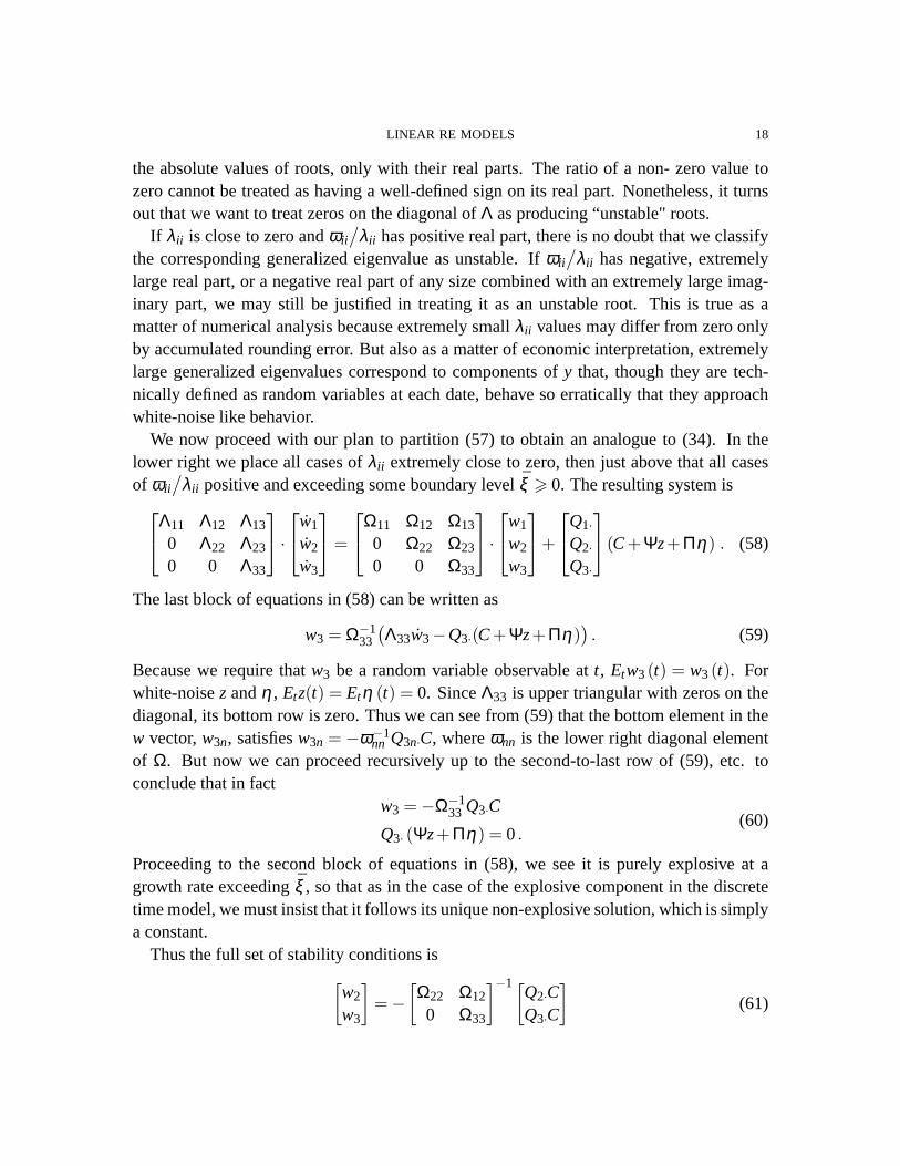
the absolute values of roots, only with their real parts. The ratio of a non- zero value tozero cannot be treated as having a well-defined sign on its real part. Nonetheless, it turnsout that we want to treat zeros on the diagonal ofΛ as producing “unstable" roots.

If λii is close to zero andωii/

λii has positive real part, there is no doubt that we classifythe corresponding generalized eigenvalue as unstable. Ifωii

/λii has negative, extremely

large real part, or a negative real part of any size combined with an extremely large imag-inary part, we may still be justified in treating it as an unstable root. This is true as amatter of numerical analysis because extremely smallλii values may differ from zero onlyby accumulated rounding error. But also as a matter of economic interpretation, extremelylarge generalized eigenvalues correspond to components ofy that, though they are tech-nically defined as random variables at each date, behave so erratically that they approachwhite-noise like behavior.

We now proceed with our plan to partition(57) to obtain an analogue to(34). In thelower right we place all cases ofλii extremely close to zero, then just above that all casesof ωii

/λii positive and exceeding some boundary levelξ > 0. The resulting system is

Λ11 Λ12 Λ13

0 Λ22 Λ23

0 0 Λ33

·

w1

w2

w3

=

Ω11 Ω12 Ω13

0 Ω22 Ω23

0 0 Ω33

·

w1

w2

w3

+

Q1·Q2·Q3·

(C+Ψz+Πη) . (58)

The last block of equations in(58) can be written as

w3 = Ω−133

(Λ33w3−Q3·(C+Ψz+Πη)

). (59)

Because we require thatw3 be a random variable observable att, Etw3(t) = w3(t). Forwhite-noisez andη , Etz(t) = Etη (t) = 0. SinceΛ33 is upper triangular with zeros on thediagonal, its bottom row is zero. Thus we can see from(59) that the bottom element in thew vector,w3n, satisfiesw3n = −ω−1

nn Q3n·C, whereωnn is the lower right diagonal elementof Ω. But now we can proceed recursively up to the second-to-last row of(59), etc. toconclude that in fact

w3 =−Ω−133 Q3·C

Q3· (Ψz+Πη) = 0.(60)

Proceeding to the second block of equations in(58), we see it is purely explosive at agrowth rate exceedingξ , so that as in the case of the explosive component in the discretetime model, we must insist that it follows its unique non-explosive solution, which is simplya constant.

Thus the full set of stability conditions is[w2

w3

]=−

[Ω22 Ω12

0 Ω33

]−1[Q2·CQ3·C

](61)

LINEAR RE MODELS 19

[Q2·Q3·

](Ψz+Πη) = 0. (62)

Just as in the discrete case, we can now translate the equations and stability conditions interms ofw back in to a stable equation iny, here taking the form

y = Θ1y+Θc +Θ0z. (63)

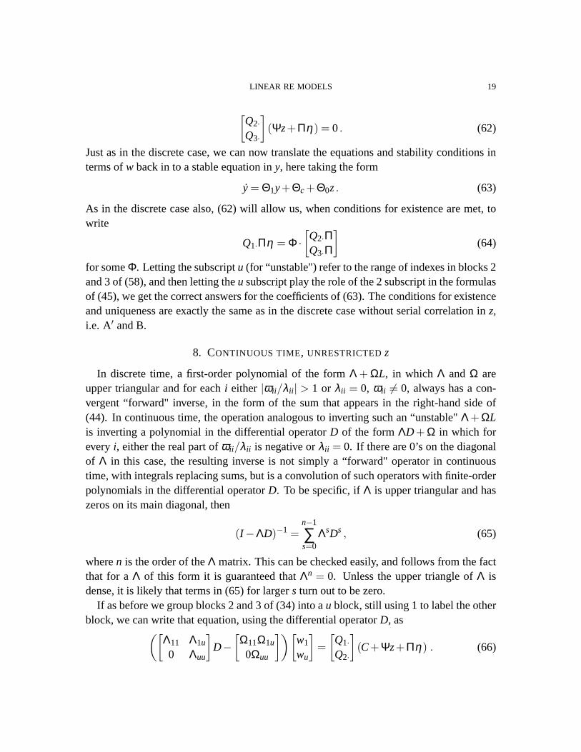
As in the discrete case also,(62) will allow us, when conditions for existence are met, towrite

Q1·Πη = Φ ·[Q2·ΠQ3·Π

](64)

for someΦ. Letting the subscriptu (for “unstable") refer to the range of indexes in blocks 2and 3 of(58), and then letting theu subscript play the role of the 2 subscript in the formulasof (45), we get the correct answers for the coefficients of(63). The conditions for existenceand uniqueness are exactly the same as in the discrete case without serial correlation inz,i.e. A′ and B.

8. CONTINUOUS TIME, UNRESTRICTEDz

In discrete time, a first-order polynomial of the formΛ + ΩL, in which Λ and Ω areupper triangular and for eachi either |ωii/λii | > 1 or λii = 0, ωii 6= 0, always has a con-vergent “forward" inverse, in the form of the sum that appears in the right-hand side of(44). In continuous time, the operation analogous to inverting such an “unstable"Λ + ΩLis inverting a polynomial in the differential operatorD of the formΛD + Ω in which foreveryi, either the real part ofωii/λii is negative orλii = 0. If there are 0’s on the diagonalof Λ in this case, the resulting inverse is not simply a “forward" operator in continuoustime, with integrals replacing sums, but is a convolution of such operators with finite-orderpolynomials in the differential operatorD. To be specific, ifΛ is upper triangular and haszeros on its main diagonal, then

(I −ΛD)−1 =n−1

∑s=0

ΛsDs , (65)

wheren is the order of theΛ matrix. This can be checked easily, and follows from the factthat for aΛ of this form it is guaranteed thatΛn = 0. Unless the upper triangle ofΛ isdense, it is likely that terms in (65) for largers turn out to be zero.

If as before we group blocks 2 and 3 of(34) into au block, still using 1 to label the otherblock, we can write that equation, using the differential operatorD, as

([Λ11 Λ1u

0 Λuu

]D−

[Ω11Ω1u

0Ωuu

])[w1

wu

]=

[Q1·Q2·

](C+Ψz+Πη) . (66)

LINEAR RE MODELS 20

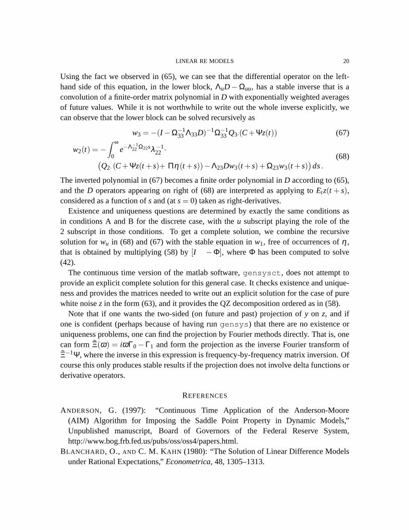
Using the fact we observed in(65), we can see that the differential operator on the left-hand side of this equation, in the lower block,ΛuD−Ωuu, has a stable inverse that is aconvolution of a finite-order matrix polynomial inD with exponentially weighted averagesof future values. While it is not worthwhile to write out the whole inverse explicitly, wecan observe that the lower block can be solved recursively as

w3 =−(I −Ω−133 Λ33D)−1Ω−1

33 Q3·(C+Ψz(t)) (67)

w2(t) =−∫ ∞

0e−Λ−1

22 Ω22sλ−122 ·

(Q2· (C+Ψz(t +s)+ Πη(t +s))−Λ23Dw3(t +s)+Ω23w3(t +s)

)ds.

(68)

The inverted polynomial in(67) becomes a finite order polynomial inD according to (65),and theD operators appearing on right of(68) are interpreted as applying toEtz(t + s),considered as a function ofs and (ats= 0) taken as right-derivatives.

Existence and uniqueness questions are determined by exactly the same conditions asin conditions A and B for the discrete case, with theu subscript playing the role of the2 subscript in those conditions. To get a complete solution, we combine the recursivesolution forwu in (68) and (67) with the stable equation inw1, free of occurrences ofη ,that is obtained by multiplying(58) by [I −Φ], whereΦ has been computed to solve(42).

The continuous time version of the matlab software,gensysct , does not attempt toprovide an explicit complete solution for this general case. It checks existence and unique-ness and provides the matrices needed to write out an explicit solution for the case of purewhite noisez in the form(63), and it provides the QZ decomposition ordered as in(58).

Note that if one wants the two-sided (on future and past) projection ofy on z, and ifone is confident (perhaps because of having rungensys ) that there are no existence oruniqueness problems, one can find the projection by Fourier methods directly. That is, onecan formΞ(ω) = iωΓ0−Γ1 and form the projection as the inverse Fourier transform ofΞ−1Ψ, where the inverse in this expression is frequency-by-frequency matrix inversion. Ofcourse this only produces stable results if the projection does not involve delta functions orderivative operators.

REFERENCES

ANDERSON, G. (1997): “Continuous Time Application of the Anderson-Moore(AIM) Algorithm for Imposing the Saddle Point Property in Dynamic Models,”Unpublished manuscript, Board of Governors of the Federal Reserve System,http://www.bog.frb.fed.us/pubs/oss/oss4/papers.html.

BLANCHARD , O., AND C. M. KAHN (1980): “The Solution of Linear Difference Modelsunder Rational Expectations,”Econometrica, 48, 1305–1313.

LINEAR RE MODELS 21

K ING, R. G., AND M. WATSON (1997): “System Reduction and SolutionAlgorithms for Singular Linear Difference Systems Under Rational Expecta-tions,” unpublished manuscript, University of Virginia and Princeton University,http://www.people.Virginia.EDU/ rgk4m/abstracts/algor.htm.

(1998): “The Solution of Singular Linear Difference Systems Under RationalExpectations,”International Economic Review.

KLEIN , P. (1997): “Using the Generalized Schur Form to Solve a System of LinearExpectational Difference Equations,” discussion paper, IIES, Stockholm University,klein@iies.su.se.

DEPARTMENT OFECONOMICS, YALE UNIVERSITY

E-mail address: sims@econ.yale.edu