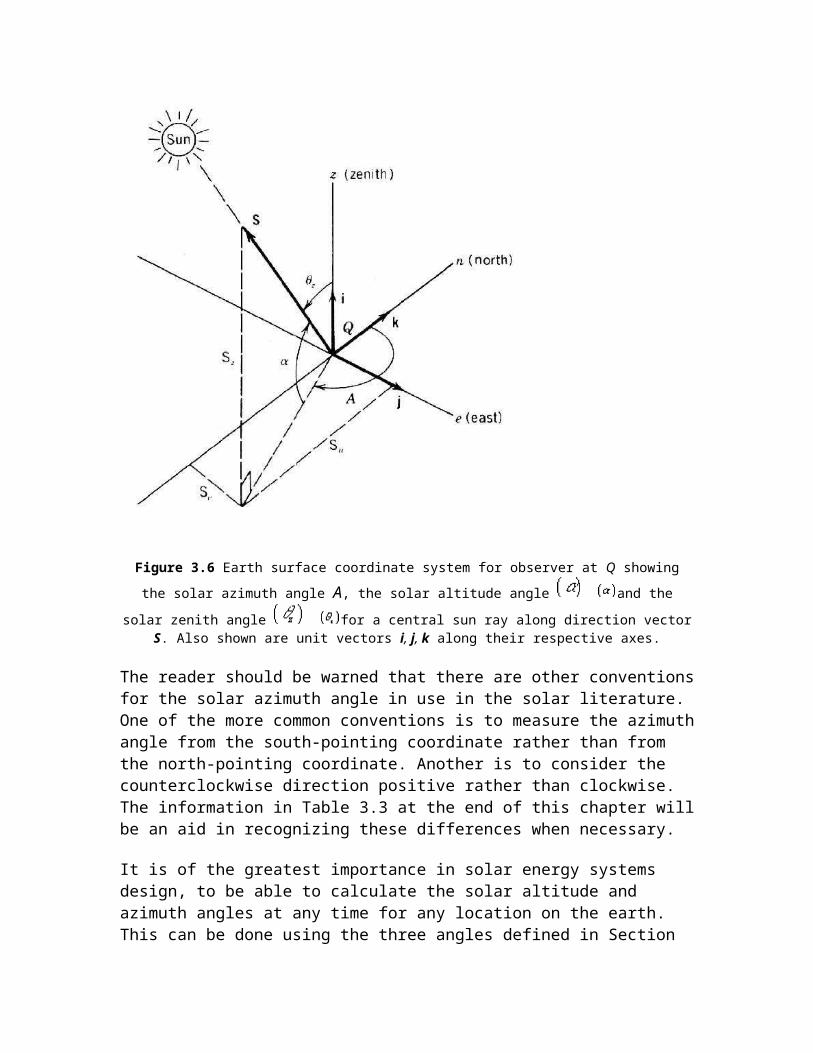
Figure 3.6 Earth surface coordinate system for observer at Q showing the solar azimuth angle Α,

the solar altitude angle and the solar zenith angle for a central sun ray along direction vector S. Also shown are unit vectors i, j, k along their respective axes.

The reader should be warned that there are other conventions for the solar azimuth angle in use in the solar literature. One of the more common conventions is to measure the azimuth angle from the south-pointing coordinate rather than from the north-pointing coordinate. Another is to consider the counterclockwise direction positive rather than clockwise. The information in Table 3.3 at the end of this chapter will be an aid in recognizing these differences when necessary.

It is of the greatest importance in solar energy systems design, to be able to calculate the solar altitude and azimuth angles at any time for any location on the earth. This can be done using the three angles defined in Section 3.1 above;

latitude , hour angle , and declination . If the reader is not interested in the details of this derivation, they are invited to skip directly to the results; Equations (3.17), (3.18) and (3.19).

For this derivation, we will define a sun-pointing vector at the surface of the earth and then mathematically translate it to the center of the earth with a different

coordinate system. Using Figure 3.6 as a guide, define a unit direction vector S pointing toward the sun from the observer location Q:

where i, j, and k are unit vectors along the z, e, and n axes respectively. The direction cosines of S relative to the z, e, and n axes are Sz, Se and Sn, respectively. These may be written in terms of solar altitude and azimuth as

Similarly, a direction vector pointing to the sun can be described at the center of the earth as shown in

Figure 3.7. If the origin of a new set of coordinates is defined at the earth’s center, the m axis can be a line from the origin intersecting the equator at the point where the meridian of the observer at Q crosses. The e axis is perpendicular to the m axis and is also in the equatorial plane. The third orthogonal axis p may then be aligned with the earth’s axis of rotation. A new direction vector S´ pointing to the sun may be described in terms of its direction cosines S´m , S'e and S'p relative to the m, e, and p axes, respectively. Writing these in terms of the declination and hour angles, we have

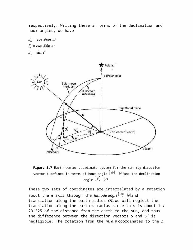
Figure 3.7 Earth center coordinate system for the sun ray direction vector S defined in terms of

hour angle and the declination angle .

These two sets of coordinates are interrelated by a rotation about the e axis

through the latitude angle and translation along the earth radius QC. We will neglect the translation along the earth’s radius since this is about 1 / 23,525 of the distance from the earth to the sun, and thus the difference between the direction vectors S and S´ is negligible. The rotation from the m, e, p coordinates to the z, e, n coordinates, about the e axis is depicted in Figure 3.8. Both sets of coordinates are summarized in Figure 3.9. Note that this rotation about the e axis is in the negative sense based on the right-hand rule. In matrix notation, this takes the form

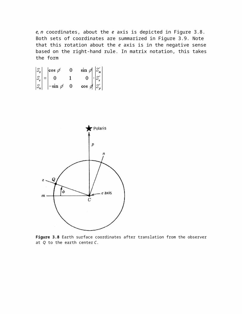
Figure 3.8 Earth surface coordinates after translation from the observer at Q to the earth center C.

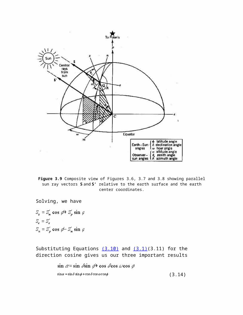
Figure 3.9 Composite view of Figures 3.6, 3.7 and 3.8 showing parallel sun ray vectors S and S’ relative to the earth surface and the earth center coordinates.

Solving, we have

Substituting Equations (3.10) and (3.1)(3.11) for the direction cosine gives us our three important results

                     (3.14)

                     (3.15)

     

Equation (3.14) is an expression for the solar altitude angle in terms of the observer’s latitude (location), the hour angle (time), and the sun’s declination

(date). Solving for the solar altitude angle , we have

                     (3.17)

Two equivalent expressions result for the solar azimuth angle (A) from either Equation (3.15) or (3.16). To reduce the number of variables, we could substitute Equation (3.14) into either Equation (3.15) or (3.16); however, this substitution results in additional terms and is often omitted to enhance computational speed in computer codes.

The solar azimuth angle can be in any of the four trigonometric quadrants depending on location, time of day, and the season. Since the arc sine and arc cosine functions have two possible quadrants for their result, both Equations (3.15) and (3.16) require a test to ascertain the proper quadrant. No such test is required for the solar altitude angle, since this angle exists in only one quadrant.

The appropriate procedure for solving Equation (3.15) is to test the result to determine whether the time is before or after solar noon. For Equation (3.15), a test must be made to determine whether the solar azimuth is north or south of the east-west line.

Two methods for calculating the solar azimuth (A), including the appropriate tests, are given by the following equations. Again, these are written for the azimuth angle sign convention used in this text, that is, that the solar azimuth angle is measured from due north in a clockwise direction, as with compass directions. Solving Equation (3.15) the untested result, A’ then becomes

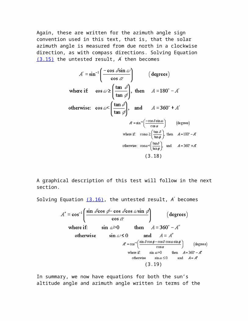
                     (3.18)

 

A graphical description of this test will follow in the next section.

Solving Equation (3.16), the untested result, A" becomes

                     (3.19)

In summary, we now have equations for both the sun’s altitude angle and azimuth angle written in terms of the latitude, declination and hour angles. This now permits us to calculate the sun’s position in the sky, as a function of date,

time and location (N, , ).

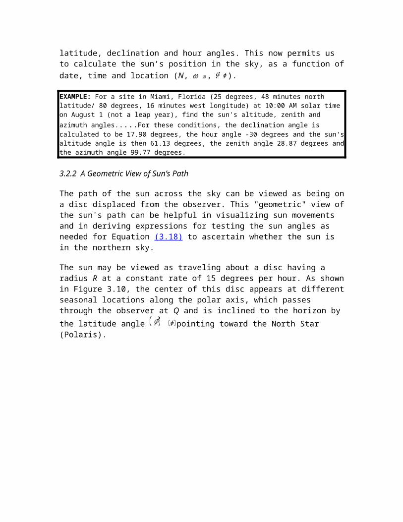
EXAMPLE: For a site in Miami, Florida (25 degrees, 48 minutes north latitude/ 80 degrees, 16 minutes west longitude) at 10:00 AM solar time on August 1 (not a leap year), find the sun's altitude, zenith and azimuth angles.....For these conditions, the declination angle is calculated to be 17.90 degrees, the hour angle -30 degrees and the sun's altitude angle is then 61.13 degrees, the zenith angle 28.87 degrees and the azimuth angle 99.77 degrees.

3.2.2  A Geometric View of Sun’s Path

The path of the sun across the sky can be viewed as being on a disc displaced from the observer. This "geometric" view of the sun's path can be helpful in visualizing sun movements and in deriving expressions for testing the sun angles as needed for Equation (3.18) to ascertain whether the sun is in the northern sky.

The sun may be viewed as traveling about a disc having a radius R at a constant rate of 15 degrees per hour. As shown in Figure 3.10, the center of this disc appears at different seasonal locations along the polar axis, which passes

through the observer at Q and is inclined to the horizon by the latitude angle

pointing toward the North Star (Polaris).

Figure 3.10 A geometric view of the sun’s path as seen by an observer at Q. Each disc has radius R.

The center of the disc is coincident with the observer Q at the equinoxes and is

displaced from the observer by a distance of at other times of the year. The extremes of this travel are at the solstices when the disc is displaced by ± 0.424 R along the polar axis. It can be seen that in the winter, much of the disc is "submerged" below the horizon, giving rise to fewer hours of daylight and low sun elevations as viewed from Q.

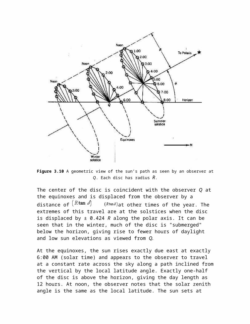
At the equinoxes, the sun rises exactly due east at exactly 6:00 AM (solar time) and appears to the observer to travel at a constant rate across the sky along a path inclined from the vertical by the local latitude angle. Exactly one-half of the disc is above the horizon, giving the day length as 12 hours. At noon, the observer notes that the solar zenith angle is the same as the local latitude. The sun sets at exactly 6:00 PM, at a solar azimuth angle of exactly 270 degrees or due west.

In the summer, the center of the disc is above the observer, giving rise to more hours of daylight and higher solar altitude angles, with the sun appearing in the northern part of the sky in the mornings and afternoons.

Since the inclination of the polar axis varies with latitude it can be visualized that there are some latitudes where the summer solstice disc is completely above the horizon surface. It can be shown that this occurs for latitudes greater than 66.55 degrees, that is, above the Arctic Circle. At the equator, the polar axis is horizontal and exactly half of any disc appears above the horizon surface, which means that the length of day and night is 12 hours throughout the year.

A test to determine whether the sun is in the northern part of the sky may be developed by use of this geometry. Figure 3.11 is a side view of the sun’s disc looking from the east.

Figure 3.11 Side view of sun path disc during the summer when the disc center Y is above the observer at Q.

In the summer the sun path disc of radius R has its center Y displaced above the observer Q. Point X is defined by a perpendicular from Q. In the n - z plane, the

projection of the position S onto the line containing X and Y will be

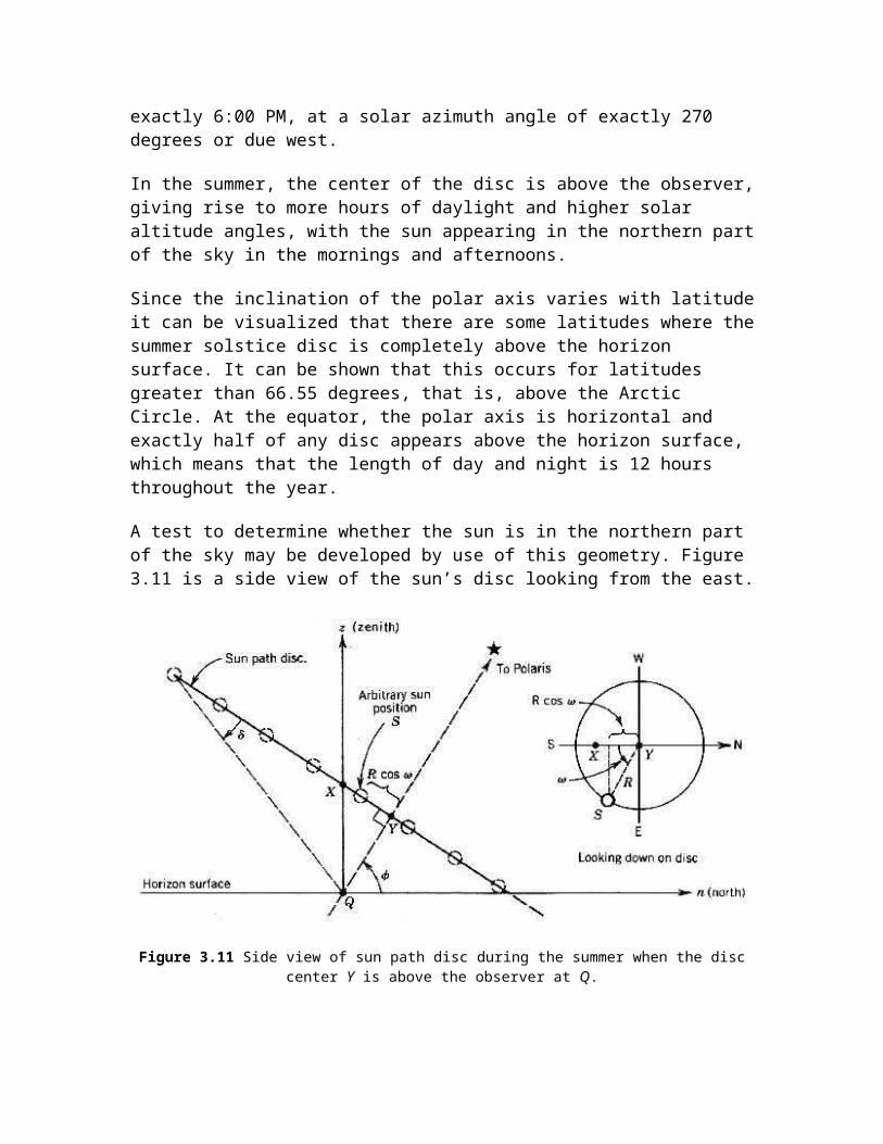
where is the hour angle. The appropriate test for the sun being in the northern sky is then

                     (3.20)

The distance XY can be found by geometry arguments. Substituting into Equation (3.20), we have

                     (3.21)

This is the test applied to Equation (3.18) to ensure that computed solar azimuth angles are in the proper quadrant.

3.2.3 Daily and Seasonal Events

Often the solar designer will want to predict the time and location of sunrise and sunset, the length of day, and the maximum solar altitude. Expressions for these are easily obtained by substitutions into expressions developed in Section 3.2. l.

The hour angle for sunset (and sunrise) may be obtained from Equation (3.17) by substituting the condition that the solar altitude at sunset equals the angle to the horizon. If the local horizon is flat, the solar altitude is zero at sunset and the hour angle at sunset becomes

                     (3.22)

The above two tests relate only to latitudes beyond 66.55 degrees, i.e. above the Arctic Circle or below the Antarctic Circle.

If the hour angle at sunset is known, this may be substituted into Equation (3.18) or (3.19) to ascertain the solar azimuth at sunrise or sunset.

The hours of daylight, sometimes of interest to the solar designer, may be calculated as

                     (3.23)

where ωs is in degrees. It is of interest to note here that although the hours of daylight vary from month to month except at the equator (where

), there are always 4,380 hours of daylight in a year (non leap year) at any location on the earth.

Another limit that may be obtained is the maximum and minimum noontime solar

altitude angle. Substitution of a value of into Equation (3.17) gives

                     (3.24)

where denotes the absolute value of this difference. An interpretation of Equation (3.24) shows that at solar noon, the solar zenith angle (the complement of the solar altitude angle) is equal to the latitude angle at the equinoxes and varies by ±23.45 degrees from summer solstice to winter solstice.

EXAMPLE: At a latitude of 35 degrees on the summer solstice (June 21), find the solar time of sunrise and sunset, the hours of daylight, the maximum solar altitude and the compass direction of the sun at sunrise and sunset.....On the summer solstice, the declination angle is +23.45 degrees, giving an hour angle at sunset of 107.68 degrees. Therefore, the time of sunrise is 4:49:17 and of sunset, 19:10:43. There are 14.36 hours of daylight that day, and the sun reaches a maximum altitude angle of 78.45 degrees. The sun rises at an azimuth angle of 60.94 degrees (north of east) and sets at an azimuth angle of 299.06 degrees (north of west).

Other seasonal maxima and minima may be determined by substituting the extremes of the declination angle, that is, ±23.45 degrees into the previously developed expressions, to obtain their values at the solstices. Since the solar designer is often interested in the limits of the sun’s movements, this tool can be very useful in developing estimates of system performance.

 

3.3 Shadows and Sundials

Now that we have developed the appropriate equations to define the direction of the sun on any day, any time and any location, let’s look at two applications, which are interesting, and may be of value to the solar designer.

3.3.1 Simple Shadows

An important use of your understanding of the sun’s position is in predicting the location of a shadow. Since sunlight travels in straight lines, the projection of an obscuring point onto the ground (or any other surface) can be described in terms of simple geometry.

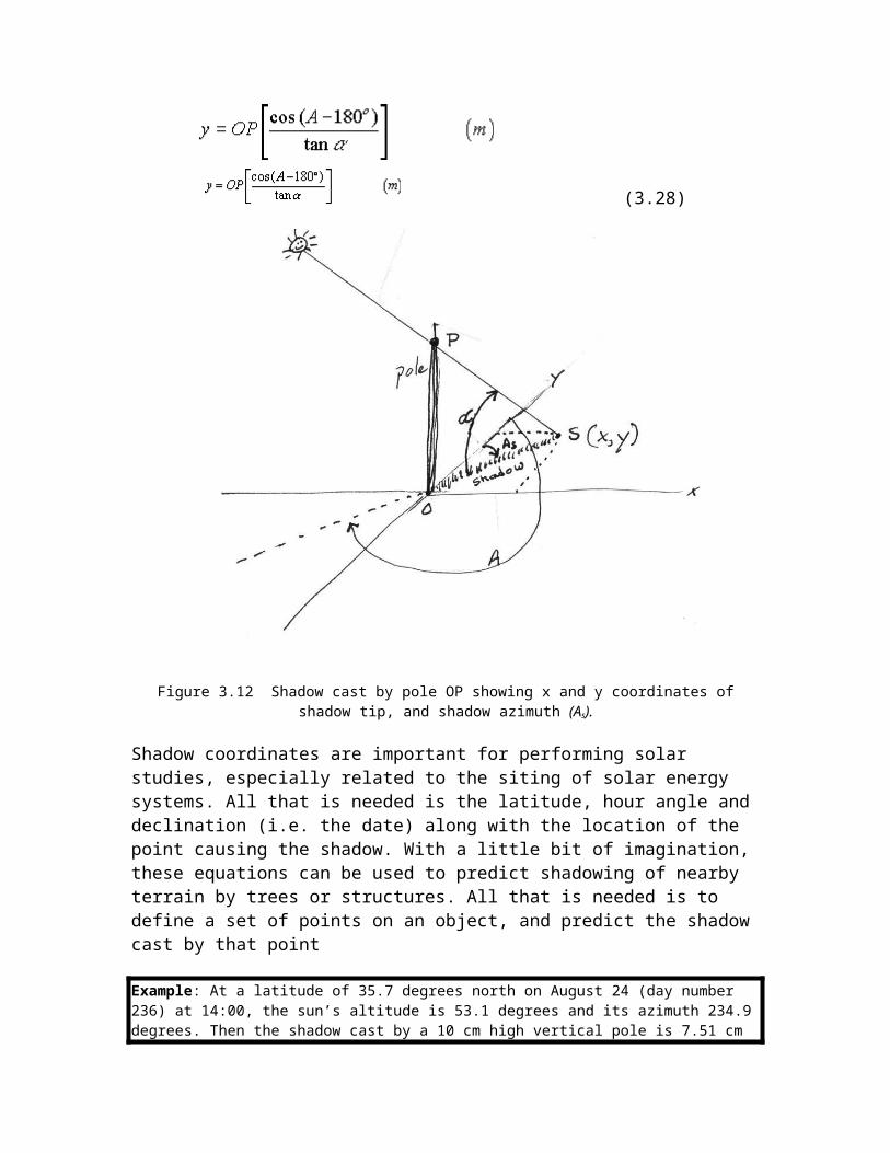
Figure 3.12 shows a vertical pole on a horizontal surface. The problem here is to define the length and direction of the shadow cast by the pole. This will first be done in terms of radial coordinates and then in Cartesian coordinates.

In polar coordinates, for a pole height, OP and the shadow azimuth, θs defined in the same manner as the previous azimuth angles i.e. relative to true north with clockwise being positive, we have for the shadow length:

                     (3.25)

and for the shadow azimuth:

                     (3.26)

In terms of Cartesian coordinates as shown on Figure 3.12, with the base of the pole as the origin, north as the positive y-direction and east the positive x-direction, the equations for the coordinates of the tip of the shadow from the vertical pole OP are:

                     (3.27)

                     (3.28)

Figure 3.12  Shadow cast by pole OP showing x and y coordinates of shadow tip, and shadow azimuth (As).

Shadow coordinates are important for performing solar studies, especially related to the siting of solar energy systems. All that is needed is the latitude, hour angle and declination (i.e. the date) along with the location of the point causing the shadow. With a little bit of imagination, these equations can be used to predict shadowing of nearby terrain by trees or structures. All that is needed is to define a set of points on an object, and predict the shadow cast by that point

Example: At a latitude of 35.7 degrees north on August 24 (day number 236) at 14:00, the sun’s altitude is 53.1 degrees and its azimuth 234.9 degrees. Then the shadow cast by a 10 cm high vertical pole is 7.51 cm long, and has a shadow azimuth (from north) of 54.9 degrees. The x- and y-coordinates of the tip of the shadow are: x = 6.14 cm and y = 4.32 cm.

3.3.1 Sundials

Throughout the history of mankind, the sun’s shadow has been used to tell he time of day. Ingenious devices casting shadows on surfaces of all shapes and orientations have been devised. However, all of these can be understood with a simple manipulation of Equations (3.25) through (3.28) developed above.

The most common sundial consists of a flat, horizontal ‘card’ with lines marked for each hour of daylight. These lines spread out from a point with the noon line

pointing toward the North Pole. A ‘gnomon’ or shadow-casting device, is mounted perpendicular to the card and along the noon line. The gnomon is

tapered at the local latitude angle, with its height increasing toward the north. Figure 3.13 below shows a simple horizontal sundial with the important angles defined.

Figure 3.13 The simple horizontal sundial

In order to derive an equation for the directions of the time lines on the card, it

must be assumed that the declination angle is zero (i.e. at the equinoxes). Using Equations (3.27) and (3.28) to define the coordinates of the shadow cast by the tip of the gnomon, and Equations (3.14), (3.15) and (3.16) to

describe these in terms of the latitude angle , and the hour angle

with the declination angle being set to zero. An expression for the angle between the gnomon shadow and its base may be derived. Through simple

geometric manipulations, the expression for this angle simplifies to

                     (3.29)

In making a horizontal sundial, it is traditional to incorporate a wise saying about time or the sun, on the sundial card. An extensive range of sources of information about sundials, their history, design and construction is available on the internet.

 

3.4 Notes on the Transformation of Vector Coordinates

A procedure used often in defining the angular relationship between a surface and the sun rays is the transformation of coordinates. Defining the vector V, we obtain

                     (3.30)

 

where i, j, and k are unit vectors collinear with the x, y, and z-axes, respectively, and the scalar coefficients (Vx, Vy, Vz) are defined along these same axes. To describe V in terms of a new set of coordinate axes x', y ', and z' with their respective unit vectors i', j' and k' in the form

                     (3.31)

we must define new scalar coefficients . Using matrix algebra will do this. A column matrix made of the original scalar coefficients representing the vector in the original coordinate system is multiplied by a matrix which defines the angle of rotation.

The result is a new column matrix representing the vector in the new coordinate system. In matrix form this operation is represented by

                     (3.32)

where Aij is defined in Figure 3.14 for rotations about the x, y, or z axis. 

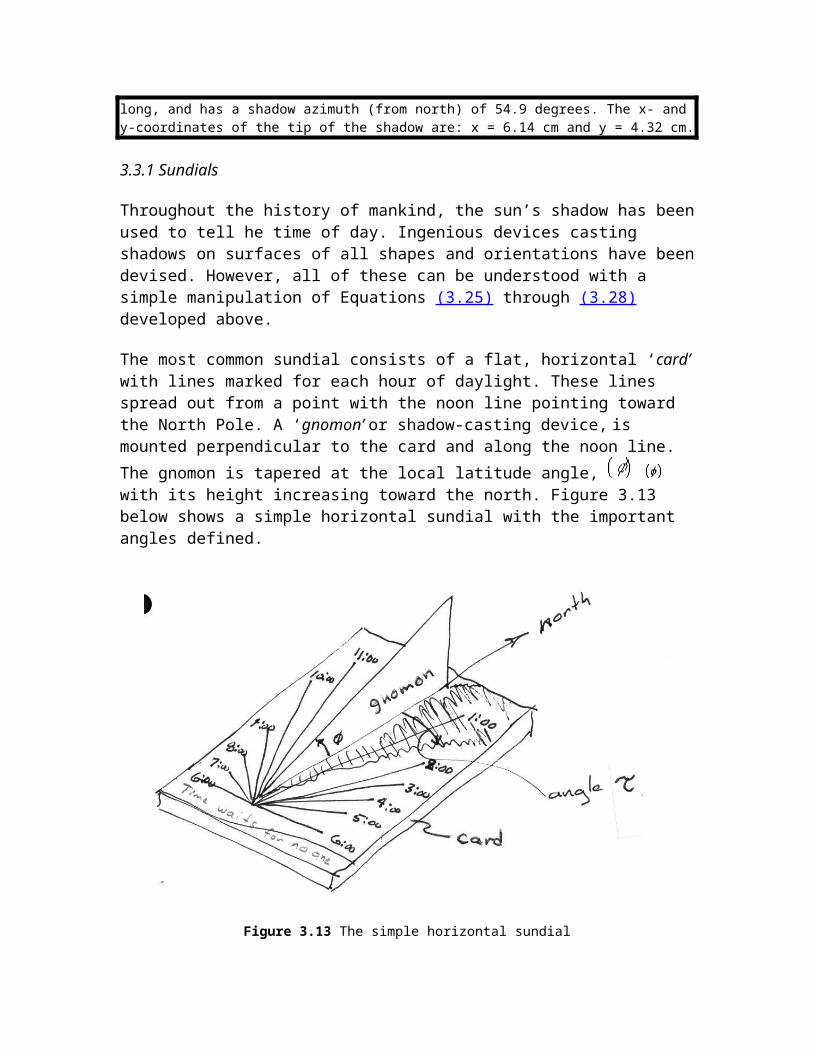
Figure 3.14 Axis rotation matrices AI j for rotation about the three principal coordinate axes by the

angle .

It should be noted here that if the magnitude of V is unity, the scalar coefficients in Equations (3.30) and (3.31) are direction cosines. Note also that the matrices given in Figure 3-22 are valid only for right-handed, orthogonal coordinate

systems, and when positive values of the angle of rotation, are determined by the right-hand rule.

Summary

Table 3.3 summarizes the angles described in this chapter along with their zero value orientation, range and sign convention.

Table 3.3   Sign Convention for Important Angles

Title Symbol ZeroPositive Direction

RangeEquation

No.Figure

No.

Earth-Sun Angles

Latitude equatornorthern

hemisphere+/- 90o --- 3.3

Declination equinox summer +/- 23.45o (3.7) 3.5

Hour Angle noon afternoon +/- 180o (3.1) 3.3

Observer-Sun Angles

Sun Altitude horizontal upward 0 to 90o (3.17) 3.6

Sun Zenith vertical toward horizon 0 to 90o (3.8) 3.6

Sun Azimuth A due north clockwise* 0 to 360o (3.18) or (3.19)

3.6

Shadow and Sundial Angles

Shadow Azimuth

As due north clockwise 0 to 360o (3.26) 3.12

Gnomon Shadow

noon afternoon +/- 180o (3.29) 3.13