Slides 12 Handout
26
Evaluation of integrals Lecture 18 Evaluation of integrals
-
Upload
santosh-reddy -
Category
Documents
-
view
237 -
download
2
description
djrj
Transcript of Slides 12 Handout
Evaluation of integrals
Lecture 18 Evaluation of integrals
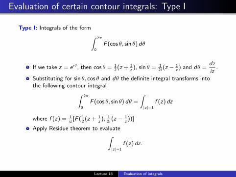
Evaluation of certain contour integrals: Type I
Type I: Integrals of the form∫ 2π
0
F (cos θ, sin θ) dθ
If we take z = e iθ, then cos θ = 12(z + 1
z), sin θ = 1
2i(z − 1
z) and dθ =
dz
iz.
Substituting for sin θ, cos θ and dθ the definite integral transforms intothe following contour integral∫ 2π
0
F (cos θ, sin θ) dθ =
∫|z|=1
f (z) dz
where f (z) = 1iz
[F ( 12(z + 1
z), 1
2i(z − 1
z))]
Apply Residue theorem to evaluate∫|z|=1
f (z) dz .
Lecture 18 Evaluation of integrals
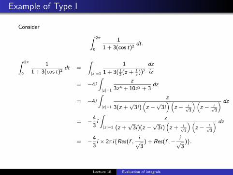
Example of Type I
Consider ∫ 2π
0
1
1 + 3(cos t)2dt.
∫ 2π
0
1
1 + 3(cos t)2dt =
∫|z|=1
1
1 + 3( 12(z + 1
z))2
dz
iz
= −4i
∫|z|=1
z
3z4 + 10z2 + 3dz
= −4i
∫|z|=1
z
3(z +√
3i)(z −√
3i)(
z + i√3
)(z − i√
3
) dz
= −4
3i
∫|z|=1
z
(z +√
3i)(z −√
3i)(z + i√
3
)(z − i√
3
) dz
= −4
3i × 2πi{Res(f ,
i√3
) + Res(f ,− i√3
)}.
Lecture 18 Evaluation of integrals
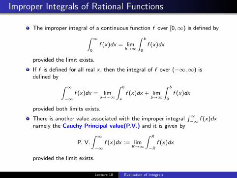
Improper Integrals of Rational Functions
The improper integral of a continuous function f over [0,∞) is defined by∫ ∞0
f (x)dx = limb→∞
∫ b
0
f (x)dx
provided the limit exists.
If f is defined for all real x , then the integral of f over (−∞,∞) isdefined by ∫ ∞
−∞f (x)dx = lim
a→−∞
∫ 0
a
f (x)dx + limb→∞
∫ b
0
f (x)dx
provided both limits exists.
There is another value associated with the improper integral∫∞−∞ f (x)dx
namely the Cauchy Principal value(P.V.) and it is given by
P. V.
∫ ∞−∞
f (x)dx := limR→∞
∫ R
−R
f (x)dx
provided the limit exists.
Lecture 18 Evaluation of integrals
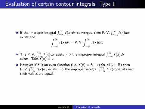
Evaluation of certain contour integrals: Type II
If the improper integral∫∞−∞ f (x)dx converges, then P. V.
∫∞−∞ f (x)dx
exists and ∫ ∞−∞
f (x)dx = P. V.
∫ ∞−∞
f (x)dx .
The P. V.∫∞−∞ f (x)dx exists 6=⇒ the improper integral
∫∞−∞ f (x)dx
exists. Take f (x) = x .
However if f is an even function (i.e. f (x) = f (−x) for all x ∈ R) thenP. V.
∫∞−∞ f (x)dx exists =⇒ the improper integral
∫∞−∞ f (x)dx exists and
their values are equal.
Lecture 18 Evaluation of integrals
Evaluation of certain contour integrals: Type II
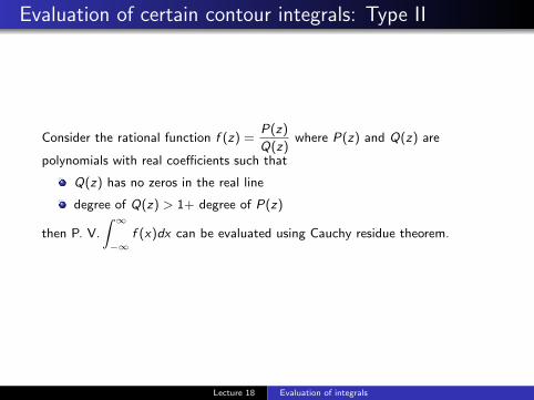
Consider the rational function f (z) =P(z)
Q(z)where P(z) and Q(z) are
polynomials with real coefficients such that
Q(z) has no zeros in the real line
degree of Q(z) > 1+ degree of P(z)
then P. V.
∫ ∞−∞
f (x)dx can be evaluated using Cauchy residue theorem.
Lecture 18 Evaluation of integrals
Evaluation of certain contour integrals: Type II
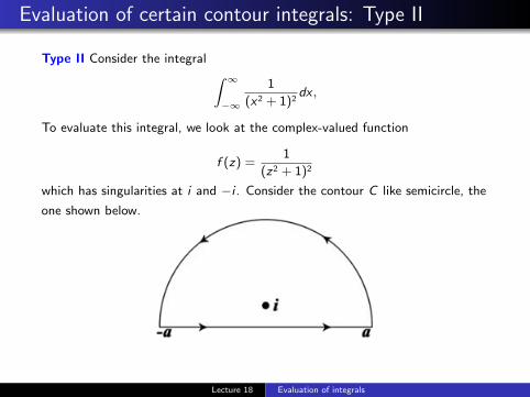
Type II Consider the integral ∫ ∞−∞
1
(x2 + 1)2dx ,
To evaluate this integral, we look at the complex-valued function
f (z) =1
(z2 + 1)2
which has singularities at i and −i . Consider the contour C like semicircle, the
one shown below.
Lecture 18 Evaluation of integrals
Evaluation of certain contour integrals: Type II
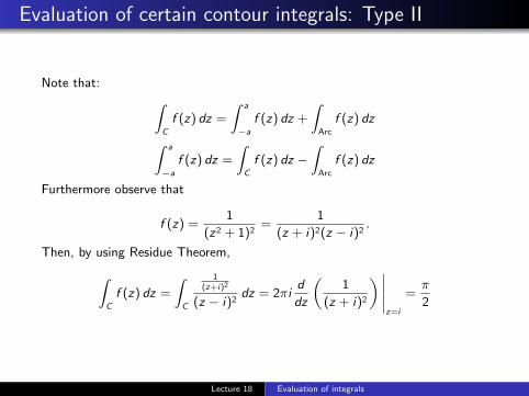
Note that: ∫C
f (z) dz =
∫ a
−a
f (z) dz +
∫Arc
f (z) dz∫ a
−a
f (z) dz =
∫C
f (z) dz −∫
Arc
f (z) dz
Furthermore observe that
f (z) =1
(z2 + 1)2=
1
(z + i)2(z − i)2.
Then, by using Residue Theorem,∫C
f (z) dz =
∫C
1(z+i)2
(z − i)2dz = 2πi
d
dz
(1
(z + i)2
) ∣∣∣∣∣z=i
=π
2
Lecture 18 Evaluation of integrals
Evaluation of certain contour integrals: Type II
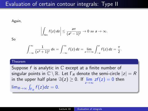
Again, ∣∣∣∣∫Arc
f (z) dz
∣∣∣∣ ≤ aπ
(a2 − 1)2→ 0 as a→∞.
So ∫ ∞−∞
1
(x2 + 1)2dx =
∫ ∞−∞
f (z) dz = lima→+∞
∫ a
−a
f (z) dz =π
2.
Theorem
Suppose f is analytic in C except at a finite number ofsingular points in C \R. Let ΓR denote the semi-circle |z | = Rin the upper half plane =(z) ≥ 0. If lim
z→∞zf (z) = 0 then
limR→∞∫
ΓRf (z)dz = 0.
Lecture 18 Evaluation of integrals
Evaluation of certain contour integrals: Type II
Exercise.
Show that P.V.
∫ ∞−∞
(x2 − x + 2)dx
(x4 + 10x2 + 9)=
5π
12. [Poles are ±i ,±3i .]
Show that
∫ ∞0
x2dx
(x2 + 9)(x2 + 4)2=
π
200.
Show that
∫ ∞0
dx
x3 + 1=
2π
3√
3.
Lecture 18 Evaluation of integrals
Evaluation of certain contour integrals: Type III
Type III Integrals of the form
P. V.
∫ ∞−∞
P(x)
Q(x)cosmx dx or P. V.
∫ ∞−∞
P(x)
Q(x)sinmx dx ,
where
P(x),Q(x) are real polynomials and m > 0
Q(x) has no zeros in the real line
degree of Q(x) > degree of P(x)
then
P. V.
∫ ∞−∞
P(x)
Q(x)cosmx dx or P. V.
∫ ∞−∞
P(x)
Q(x)sinmx dx
can be evaluated using Cauchy residue theorem.
Lecture 18 Evaluation of integrals
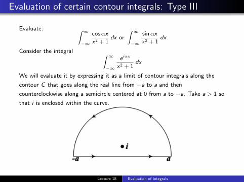
Evaluation of certain contour integrals: Type III
Evaluate: ∫ ∞−∞
cosαx
x2 + 1dx or
∫ ∞−∞
sinαx
x2 + 1dx
Consider the integral ∫ ∞−∞
e iαx
x2 + 1dx
We will evaluate it by expressing it as a limit of contour integrals along the
contour C that goes along the real line from −a to a and then
counterclockwise along a semicircle centered at 0 from a to −a. Take a > 1 so
that i is enclosed within the curve.
Lecture 18 Evaluation of integrals
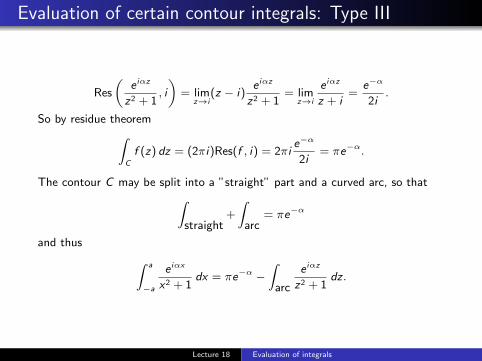
Evaluation of certain contour integrals: Type III
Res
(e iαz
z2 + 1, i
)= lim
z→i(z − i)
e iαz
z2 + 1= lim
z→i
e iαz
z + i=
e−α
2i.
So by residue theorem∫C
f (z) dz = (2πi)Res(f , i) = 2πie−α
2i= πe−α.
The contour C may be split into a ”straight” part and a curved arc, so that∫straight
+
∫arc
= πe−α
and thus ∫ a
−a
e iαx
x2 + 1dx = πe−α −
∫arc
e iαz
z2 + 1dz .
Lecture 18 Evaluation of integrals
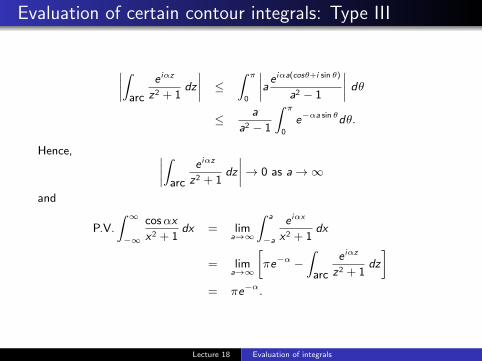
Evaluation of certain contour integrals: Type III
∣∣∣∣∫arc
e iαz
z2 + 1dz
∣∣∣∣ ≤ ∫ π
0
∣∣∣∣a e iαa(cosθ+i sin θ)
a2 − 1
∣∣∣∣ dθ≤ a
a2 − 1
∫ π
0
e−αa sin θdθ.
Hence, ∣∣∣∣∫arc
e iαz
z2 + 1dz
∣∣∣∣→ 0 as a→∞
and
P.V.
∫ ∞−∞
cosαx
x2 + 1dx = lim
a→∞
∫ a
−a
e iαx
x2 + 1dx
= lima→∞
[πe−α −
∫arc
e iαz
z2 + 1dz
]= πe−α.
Lecture 18 Evaluation of integrals
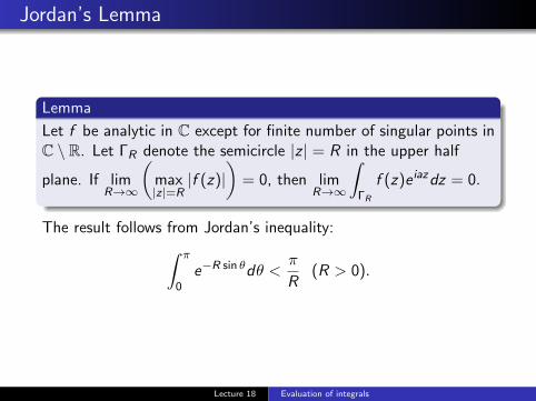
Jordan’s Lemma
Lemma
Let f be analytic in C except for finite number of singular points inC \ R. Let ΓR denote the semicircle |z | = R in the upper half
plane. If limR→∞
(max|z|=R
|f (z)|)
= 0, then limR→∞
∫ΓR
f (z)e iazdz = 0.
The result follows from Jordan’s inequality:∫ π
0e−R sin θdθ <
π
R(R > 0).
Lecture 18 Evaluation of integrals
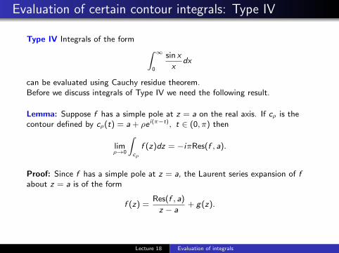
Evaluation of certain contour integrals: Type IV
Type IV Integrals of the form ∫ ∞0
sin x
xdx
can be evaluated using Cauchy residue theorem.Before we discuss integrals of Type IV we need the following result.
Lemma: Suppose f has a simple pole at z = a on the real axis. If cρ is thecontour defined by cρ(t) = a + ρe i(π−t), t ∈ (0, π) then
limρ→0
∫cρ
f (z)dz = −iπRes(f , a).
Proof: Since f has a simple pole at z = a, the Laurent series expansion of fabout z = a is of the form
f (z) =Res(f , a)
z − a+ g(z).
Lecture 18 Evaluation of integrals
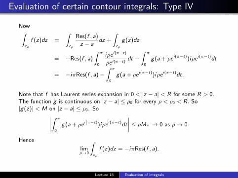
Evaluation of certain contour integrals: Type IV
Now∫cρ
f (z)dz =
∫cρ
Res(f , a)
z − adz +
∫cρ
g(z)dz
= −Res(f , a)
∫ π
0
iρe i(π−t)
ρe i(π−t)dt −
∫ π
0
g(a + ρe i(π−t))iρe i(π−t)dt
= −iπRes(f , a)−∫ π
0
g(a + ρe i(π−t))iρe i(π−t)dt.
Note that f has Laurent series expansion in 0 < |z − a| < R for some R > 0.The function g is continuous on |z − a| ≤ ρ0 for every ρ < ρ0 < R. So|g(z)| < M on |z − a| ≤ ρ0. So∣∣∣∣∫ π
0
g(a + ρe i(π−t))iρe i(π−t)dt
∣∣∣∣ ≤ ρMπ → 0 as ρ→ 0.
Hence
limρ→0
∫cρ
f (z)dz = −iπRes(f , a).
Lecture 18 Evaluation of integrals
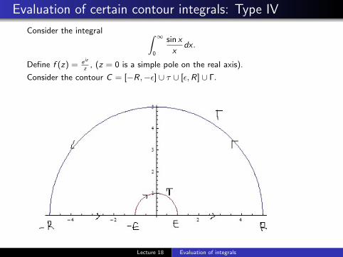
Evaluation of certain contour integrals: Type IV
Consider the integral ∫ ∞0
sin x
xdx .
Define f (z) = e iz
z, (z = 0 is a simple pole on the real axis).
Consider the contour C = [−R,−ε] ∪ τ ∪ [ε,R] ∪ Γ.
Lecture 18 Evaluation of integrals
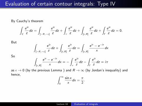
Evaluation of certain contour integrals: Type IV
By Cauchy’s theorem∫C
e iz
zdz =
∫[−R,−ε]
e iz
zdz +
∫τ
e iz
zdz +
∫[ε,R]
e iz
zdz +
∫Γ
e iz
zdz = 0.
But ∫[−R,−ε]
e iz
zdz +
∫[ε,R]
e iz
zdz =
∫[ε,R]
e ix − e−ix
xdx
So ∫[ε,R]
e ix − e−ix
xdx = −
∫τ
e iz
zdz −
∫Γ
e iz
zdz = iπ
as ε→ 0 (by the previous Lemma ) and R →∞ (by Jordan’s inequality) andhence, ∫ ∞
0
sin x
xdx =
π
2.
Lecture 18 Evaluation of integrals
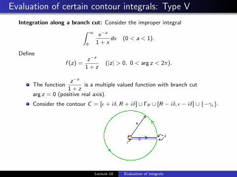
Evaluation of certain contour integrals: Type V
Integration along a branch cut: Consider the improper integral∫ ∞0
x−a
1 + xdx (0 < a < 1).
Define
f (z) =z−a
1 + z(|z | > 0, 0 < arg z < 2π).
The functionz−a
1 + zis a multiple valued function with branch cut
arg z = 0 (positive real axis).
Consider the contour C = [ε+ iδ,R + iδ] ∪ ΓR ∪ [R − iδ, ε− iδ] ∪ {−γε}.
Lecture 18 Evaluation of integrals
Evaluation of certain contour integrals: Type V
By residue theorem(∫[ε+iδ,R+iδ]
+
∫ΓR
+
∫[R−iδ,ε−iδ]
+
∫−γε
)f (z)dz = 2πiRes(f ,−1) = 2πie−iaπ.
Since
f (z) =exp(−a log z)
z + 1=
exp(−a(ln r + iθ))
re iθ + 1,
where z = re iθ, it follows thatOn [ε+ iδ,R + iδ], θ → 0 as δ → 0,
f (z) =exp(−a(ln r + i .0))
re i.0 + 1→ r−a
1 + ras δ → 0.
On [R − iδ, ε− iδ], θ → 2π as δ → 0,
f (z) =exp(−a(ln r + i .2π))
re i.2π + 1→ r−a
1 + re−2aπi as δ → 0.
Lecture 18 Evaluation of integrals
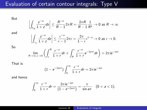
Evaluation of certain contour integrals: Type V
But ∣∣∣∣∫ΓR
z−a
1 + zdz
∣∣∣∣ ≤ R−a
R − 12πR =
2πR
R − 1
1
Ra→ 0 as R →∞
and ∣∣∣∣∫γε
z−a
1 + zdz
∣∣∣∣ ≤ ε−a
ε− 12πε =
2π
1− ε ε1−a → 0 as ε→ 0.
So
limR→∞,ε→0
(∫ R
ε
r−a
1 + rdr +
∫ ε
R
r−a
1 + re−2aπidr
)= 2πie−iaπ
That is
(1− e−2aπi )
∫ ∞0
r−a
1 + rdr = 2πie−iaπ
and hence ∫ ∞0
r−a
1 + rdr =
2πie−iaπ
(1− e−2aπi )=
π
sin aπ(0 < a < 1).
Lecture 18 Evaluation of integrals
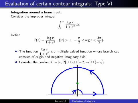
Evaluation of certain contour integrals: Type VI
Integration around a branch cut:Consider the improper integral ∫ ∞
0
log x
1 + x2dx .
Define
f (z) =log z
1 + z2(|z | > 0, − π
2< arg z <
3π
2).
The functionlog z
1 + z2is a multiple valued function whose branch cut
consists of origin and negative imaginary axis.
Consider the contour C = [ε,R] ∪ ΓR ∪ [−R,−ε] ∪ {−γε}.
Lecture 18 Evaluation of integrals
Evaluation of certain contour integrals: Type VI
By Cauchy’s residue theorem(∫[ε,R]
+
∫ΓR
+
∫[−R,−ε]
+
∫−γε
)f (z)dz = 2πiRes(f , i) = 2πi
π
4=π2i
2.
Since
f (z) =log z
z2 + 1=
log |z |+ iθ
r 2e2iθ + 1,
where z = re iθ, it follows thatOn [ε,R], θ = 0,
f (z) =log x
x2 + 1.
On [−R,−ε], θ = π,
f (z) =log |x |+ iπ
x2 + 1.
Lecture 18 Evaluation of integrals
Evaluation of certain contour integrals: Type VI
But ∣∣∣∣∫ΓR
log z
1 + z2dz
∣∣∣∣ =
∣∣∣∣∫ΓR
logR + iθ
1 + R2e2iθiRe iθdθ
∣∣∣∣≤ R
| logR|R2 − 1
π +R
R2 − 1
∫ π
0
θdθ → 0
as R →∞ and∣∣∣∣∫γε
log z
1 + z2dz
∣∣∣∣ =
∣∣∣∣∫γε
log ε+ iθ
1 + ε2e2iθiεe iθdθ
∣∣∣∣≤ επ
| log ε|ε2 − 1
+ε
ε2 − 1
∫ π
0
θdθ → 0 as ε→ 0.
Lecture 18 Evaluation of integrals
Evaluation of certain contour integrals: Type VI
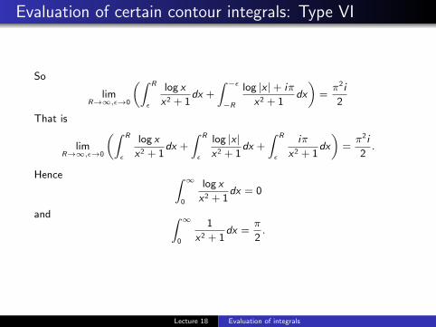
So
limR→∞,ε→0
(∫ R
ε
log x
x2 + 1dx +
∫ −ε−R
log |x |+ iπ
x2 + 1dx
)=π2i
2
That is
limR→∞,ε→0
(∫ R
ε
log x
x2 + 1dx +
∫ R
ε
log |x |x2 + 1
dx +
∫ R
ε
iπ
x2 + 1dx
)=π2i
2.
Hence ∫ ∞0
log x
x2 + 1dx = 0
and ∫ ∞0
1
x2 + 1dx =
π
2.
Lecture 18 Evaluation of integrals