Simultaneous measurement of 13C, 18O and 17 of atmospheric ...
26
Atmos. Meas. Tech., 14, 4279–4304, 2021 https://doi.org/10.5194/amt-14-4279-2021 © Author(s) 2021. This work is distributed under the Creative Commons Attribution 4.0 License. Simultaneous measurement of δ 13 C, δ 18 O and δ 17 O of atmospheric CO 2 – performance assessment of a dual-laser absorption spectrometer Pharahilda M. Steur 1 , Hubertus A. Scheeren 1 , Dave D. Nelson 2 , J. Barry McManus 2 , and Harro A. J. Meijer 1 1 Centre for Isotope Research, University of Groningen, Nijenborgh 6, 9747 AG Groningen, the Netherlands 2 Aerodyne Research Inc., 45 Manning Road, Billerica, MA 01821-3976, USA Correspondence: Pharahilda M. Steur ([email protected]) Received: 9 September 2020 – Discussion started: 12 November 2020 Revised: 17 April 2021 – Accepted: 21 April 2021 – Published: 9 June 2021 Abstract. Using laser absorption spectrometry for the mea- surement of stable isotopes of atmospheric CO 2 instead of the traditional isotope ratio mass spectrometry method de- creases sample preparation time significantly, and uncertain- ties in the measurement accuracy due to CO 2 extraction and isobaric interferences are avoided. In this study we present the measurement performance of a new dual-laser instru- ment developed for the simultaneous measurement of the δ 13 C, δ 18 O and δ 17 O of atmospheric CO 2 in discrete air sam- ples, referred to as the Stable Isotopes of CO 2 Absorption Spectrometer (SICAS). We compare two different calibration methods: the ratio method, based on the measured isotope ra- tio and a CO 2 mole fraction dependency correction, and the isotopologue method, based on measured isotopologue abun- dances. Calibration with the ratio method and isotopologue method is based on three different assigned whole-air refer- ences calibrated on the VPDB (Vienna Pee Dee Belemnite) and the WMO 2007 (World Meteorological Organization) scale for their stable isotope compositions and their CO 2 mole fractions, respectively. An additional quality control tank is included in both methods to follow long-term instru- ment performance. Measurements of the quality control tank show that the measurement precision and accuracy of both calibration methods is of similar quality for δ 13 C and δ 18 O measurements. During one specific measurement period the precision and accuracy of the quality control tank reach WMO compatibility requirements, being 0.01 ‰ for δ 13 C and 0.05 ‰ for δ 18 O. Uncertainty contributions of the scale uncertainties of the reference gases add another 0.03 ‰ and 0.05 ‰ to the combined uncertainty of the sample measure- ments. Hence, reaching WMO compatibility for sample mea- surements on the SICAS requires reduction of the scale un- certainty of the reference gases used for calibration. An in- tercomparison of flask samples over a wide range of CO 2 mole fractions has been conducted with the Max Planck In- stitute for Biogeochemistry, resulting in a mean residual of 0.01 ‰ and -0.01 ‰ and a standard deviation of 0.05 ‰ and 0.07 ‰ for the δ 13 C measurements calibrated using the ra- tio method and the isotopologue method, respectively. The δ 18 O could not be compared due to depletion of the δ 18 O signal in our sample flasks because of storage times being too long. Finally, we evaluate the potential of our 1 17 O mea- surements as a tracer for gross primary production by vegeta- tion through photosynthesis. Here, a measurement precision of < 0.01 ‰ would be a prerequisite for capturing seasonal variations in the 1 17 O signal. Lowest standard errors for the δ 17 O and 1 17 O of the ratio method and the isotopologue method are 0.02 ‰ and 0.02 ‰ and 0.01 ‰ and 0.02 ‰, re- spectively. The accuracy results show consequently results that are too enriched for both the δ 17 O and 1 17 O measure- ments for both methods. This is probably due to the fact that two of our reference gases were not measured directly but were determined indirectly. The ratio method shows resid- uals ranging from 0.06 ‰ to 0.08 ‰ and from 0.06 ‰ to 0.1 ‰ for the δ 17 O and 1 17 O results, respectively. The iso- topologue method shows residuals ranging from 0.04 ‰ to 0.1 ‰ and from 0.05 ‰ to 0.13 ‰ for the δ 17 O and 1 17 O results, respectively. Direct determination of the δ 17 O of all reference gases would improve the accuracy of the δ 17 O and thereby of the 1 17 O measurements. Published by Copernicus Publications on behalf of the European Geosciences Union.
Transcript of Simultaneous measurement of 13C, 18O and 17 of atmospheric ...
Atmos. Meas. Tech., 14, 4279–4304, 2021https://doi.org/10.5194/amt-14-4279-2021© Author(s) 2021. This work is distributed underthe Creative Commons Attribution 4.0 License.
Simultaneous measurement of δ13C, δ18O and δ17Oof atmospheric CO2 – performance assessmentof a dual-laser absorption spectrometerPharahilda M. Steur1, Hubertus A. Scheeren1, Dave D. Nelson2, J. Barry McManus2, and Harro A. J. Meijer1
1Centre for Isotope Research, University of Groningen, Nijenborgh 6, 9747 AG Groningen, the Netherlands2Aerodyne Research Inc., 45 Manning Road, Billerica, MA 01821-3976, USA
Correspondence: Pharahilda M. Steur ([email protected])
Received: 9 September 2020 – Discussion started: 12 November 2020Revised: 17 April 2021 – Accepted: 21 April 2021 – Published: 9 June 2021
Abstract. Using laser absorption spectrometry for the mea-surement of stable isotopes of atmospheric CO2 instead ofthe traditional isotope ratio mass spectrometry method de-creases sample preparation time significantly, and uncertain-ties in the measurement accuracy due to CO2 extraction andisobaric interferences are avoided. In this study we presentthe measurement performance of a new dual-laser instru-ment developed for the simultaneous measurement of theδ13C, δ18O and δ17O of atmospheric CO2 in discrete air sam-ples, referred to as the Stable Isotopes of CO2 AbsorptionSpectrometer (SICAS). We compare two different calibrationmethods: the ratio method, based on the measured isotope ra-tio and a CO2 mole fraction dependency correction, and theisotopologue method, based on measured isotopologue abun-dances. Calibration with the ratio method and isotopologuemethod is based on three different assigned whole-air refer-ences calibrated on the VPDB (Vienna Pee Dee Belemnite)and the WMO 2007 (World Meteorological Organization)scale for their stable isotope compositions and their CO2mole fractions, respectively. An additional quality controltank is included in both methods to follow long-term instru-ment performance. Measurements of the quality control tankshow that the measurement precision and accuracy of bothcalibration methods is of similar quality for δ13C and δ18Omeasurements. During one specific measurement period theprecision and accuracy of the quality control tank reachWMO compatibility requirements, being 0.01 ‰ for δ13Cand 0.05 ‰ for δ18O. Uncertainty contributions of the scaleuncertainties of the reference gases add another 0.03 ‰ and0.05 ‰ to the combined uncertainty of the sample measure-
ments. Hence, reaching WMO compatibility for sample mea-surements on the SICAS requires reduction of the scale un-certainty of the reference gases used for calibration. An in-tercomparison of flask samples over a wide range of CO2mole fractions has been conducted with the Max Planck In-stitute for Biogeochemistry, resulting in a mean residual of0.01 ‰ and−0.01 ‰ and a standard deviation of 0.05 ‰ and0.07 ‰ for the δ13C measurements calibrated using the ra-tio method and the isotopologue method, respectively. Theδ18O could not be compared due to depletion of the δ18Osignal in our sample flasks because of storage times beingtoo long. Finally, we evaluate the potential of our117O mea-surements as a tracer for gross primary production by vegeta-tion through photosynthesis. Here, a measurement precisionof < 0.01 ‰ would be a prerequisite for capturing seasonalvariations in the 117O signal. Lowest standard errors for theδ17O and 117O of the ratio method and the isotopologuemethod are 0.02 ‰ and 0.02 ‰ and 0.01 ‰ and 0.02 ‰, re-spectively. The accuracy results show consequently resultsthat are too enriched for both the δ17O and 117O measure-ments for both methods. This is probably due to the fact thattwo of our reference gases were not measured directly butwere determined indirectly. The ratio method shows resid-uals ranging from 0.06 ‰ to 0.08 ‰ and from 0.06 ‰ to0.1 ‰ for the δ17O and 117O results, respectively. The iso-topologue method shows residuals ranging from 0.04 ‰ to0.1 ‰ and from 0.05 ‰ to 0.13 ‰ for the δ17O and 117Oresults, respectively. Direct determination of the δ17O of allreference gases would improve the accuracy of the δ17O andthereby of the 117O measurements.
Published by Copernicus Publications on behalf of the European Geosciences Union.
4280 P. M. Steur et al.: Simultaneous measurement of δ13C, δ18O and δ17O of atmospheric CO2
1 Introduction
As atmospheric CO2 (atm-CO2) is the most important con-tributor to anthropogenic global warming, keeping track ofits sources and sinks is essential for understanding and pre-dicting the consequences of climate change for natural sys-tems and societies and for assessing and quantifying thepossible mitigating measures. The stable isotope (si) com-position of atm-CO2 is often used as an additional tool todistinguish between anthropogenic emissions and the influ-ence of the biosphere on varying CO2 mole fractions (Patakiet al., 2003; Zhou et al., 2005). For this reason, the si com-position of atm-CO2 is monitored at a considerable num-ber of atmospheric measurement stations around the globe.Due to the large size of the carbon reservoir of the atmo-sphere and the long lifetime of CO2 in the atmosphere, theeffects of sources and sinks on the atmospheric compositionare heavily diluted. Changes in the isotope composition ofatm-CO2 are therefore relatively small compared to the ac-tual changes in carbon fluxes (IAEA, 2002). Hence, currentclimate change and meteorological research, as well as themonitoring of CO2 emissions, require accurate and precisegreenhouse gas measurements that can meet the WMO/GAW(Global Atmosphere Watch Program of the World Meteoro-logical Organization) inter-laboratory compatibility goals of0.01 ‰ for δ13C and 0.05 ‰ for δ18O of atm-CO2 for theNorthern Hemisphere (Crotwell et al., 2020).
Traditionally, high-precision stable isotope measurementsare done using isotope ratio mass spectrometry (IRMS)(Roeloffzen et al., 1991; Trolier et al., 1996; Allison andFrancey, 1995), which requires extraction of CO2 from theair sample before a measurement is possible. This is a time-consuming process wherein very strict, 100 % extraction pro-cedures need to be applied to avoid isotope fractionation andto prevent isotope exchange of CO2 molecules with othergases or water. Extraction of CO2 from air is a major con-tributor to both random and systematic-scale differences be-tween laboratories and thus complicates the comparison ofmeasurements (Wendeberg et al., 2013). Further, due to theisobaric interferences of both different CO2 isotopologuesand N2O molecules, which are also trapped with the (cryo-genic) extraction of CO2 from air, corrections need to beapplied for the determination of the δ13C and δ18O val-ues. Due to the mass interference of the 12C17O16O isotopo-logue with 13C16O16O (and to a lesser extent 13C17O16O and12C17O17O with 12C18O16O), the δ13C results need a correc-tion (usually referred to as “ion correction”) that builds uponan assumed fixed relation between δ17O and δ18O. This as-sumed relation has varied in the past (Santrock et al., 1985;Allison et al., 1995; Assonov and Brenninkmeijer, 2003;Brand et al., 2010), again giving rise to systematic differ-ences (and confusion) between laboratories. Determinationof the δ17O of CO2 samples itself using IRMS is extremelycomplex, due to the mass overlap of the 13C and 17O con-taining isotopologues, and can only be done using very ad-
vanced techniques, restricted to just a few laboratories at themoment (see Adnew et al., 2019, and references therein). Asthe δ17O in addition to the δ18O values in atmospheric CO2have the potential to be a tracer for gross primary productionand anthropogenic emissions (Laskar et al., 2016; Luz et al.,1999; Koren et al., 2019), a less labor-intensive method thatwould enable all three stable isotopologues of atm-CO2 to beanalyzed at a sufficient precision would be an asset.
Optical (infrared) spectroscopy now offers this possibil-ity following strong developments in recent years in Fourier-transform infrared (FTIR) spectroscopy and, especially forthe laser light sources, to perform isotopologue measure-ments showing precision close to, or even surpassing, IRMSmeasurements (Tuzson et al., 2008; Vogel et al., 2013;McManus et al., 2015). The technique was developed inthe 1990s to a level where useful isotope signals could bemeasured, first on pure compounds such as water vapor (Ker-stel et al., 1999) and soon also directly on CO2 in dry whole-air samples (Becker et al., 1992; Murnick and Peer, 1994;Erdélyi et al., 2002; Gagliardi et al., 2003). Extraction ofCO2 from the air can therefore be avoided, and smallersample sizes suffice. Finally, optical spectroscopy is trulyisotopologue-specific and is thus free of isobaric interfer-ences, hence giving the possibility to directly measure theδ17O in addition to the δ13C and δ18O. Recent studies al-ready showed the effectiveness of optical spectroscopy forthe measurement of δ17O in pure CO2 for various applica-tions (Sakai et al., 2017; Stoltmann et al., 2017; Prokhorovet al., 2019).
In this paper we present the performance, in terms of pre-cision and accuracy, of an Aerodyne dual-laser optical spec-trometer (CW-IC-TILDAS-D) in use since September 2017,for the simultaneous measurement of δ13C, δ18O and δ17Oof atm-CO2, which we refer to as the Stable Isotopes of CO2Absorption Spectrometer (SICAS). The instrument perfor-mance over time is discussed, followed by an analysis of theCO2 mole fraction dependency of the instrument. We reportCO2 mole fractions in micromoles per mole (µmol mol−1),also referred to as parts per million (ppm). The actual waysof performing a calibrated measurement using either individ-ual isotopologue measurements or isotope ratios is discussed,and whole-air measurement results of both calibration meth-ods are evaluated for their compatibility with IRMS stableisotope measurements. Conclusively, the usefulness of thetriple oxygen isotope measurements for capturing signals ofatmospheric CO2 sources and sinks is evaluated.
2 Instrument description
2.1 Instrumental setup
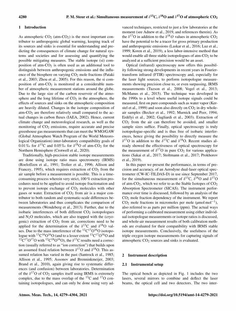
The optical bench as depicted in Fig. 1 includes the twolasers, several mirrors to combine and deflect the laserbeams, the optical cell and two detectors. The two inter-
Atmos. Meas. Tech., 14, 4279–4304, 2021 https://doi.org/10.5194/amt-14-4279-2021
P. M. Steur et al.: Simultaneous measurement of δ13C, δ18O and δ17O of atmospheric CO2 4281
Figure 1. Scheme of the optical board of the SICAS (figure adaptedfrom McManus et al., 2015). Two pathways are shown, both con-sisting of signals from both lasers: the sample measurement beamin red and the reference beam in blue. The reference pathway is inour case only used for fitting purposes. RBS stands for referencebeam splitter. One of the detectors is used to read the signal of thesample beam, the other for the reference beam. The red trace laseris co-aligned with the sample path to visualize the sample pathwayto ease alignment.
band cascade lasers (Nanoplus GmbH, Germany) operatein the mid-infrared region. The isotopologues that are mea-sured are 12C16O2, 13C16O2, 12C16O18O and 12C16O17O,which from now on will be indicated as 626, 636, 628 and627 respectively, following the HITRAN database notation(Gordon et al., 2017). Application of a small current rampcauses small frequency variations, so the lasers are swept(with a sweep frequency of 1.7 kHz) over a spectral rangein which ro-vibrational transitions of the isotopologues oc-cur with similar optical depths (Tuzson et al., 2008). Laser 1operates in the spectral range of 2350 cm−1 (4.25 µm) formeasurement of 627 (and 626), and laser 2 operates around2310 cm−1 (4.33 µm) for the measurement of 626, 636and 628. The lasers are thermoelectrically cooled and sta-bilized to temperatures of −1.1 and 9.9 ◦C, respectively. Thebeams are introduced in a multi-pass aluminum cell with avolume of 0.16 L, in which an air sample is present at lowpressure (∼ 50 mbar). The total path length of the laser lightin the optical cell is 36 m.
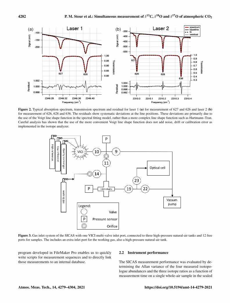
After passing the cell, the lasers are led to a thermoelectri-cally cooled infrared detector, measuring the signal from thelasers in the spectral range (Fig. 2). The lasers, optical celland detectors are all in a housing that is continuously flushedwith N2 gas to avoid any other absorption by CO2 than fromgas in the optical cell. The temperature within the housing iscontrolled using a recirculating liquid chiller set at a tempera-ture of 20 ◦C to keep the temperature in the cell stable. Withina measurement sequence (∼ 12 h) the temperature does not
normally fluctuate more than 0.05 ◦C. The absorption spec-tra are derived by the software TDLWintel (McManus et al.,2005) that fits the measured signal based on known molecu-lar absorption profiles from the HITRAN database (Rothmanet al., 2013). On the basis of the integration of the peaks atthe specific wavelengths, measured pressure and temperaturein the optical cell and the constant path length, the isotopo-logue mole fractions are calculated by the TDLWintel soft-ware with an output frequency of 1 Hz. For convenience, thedefault output for the isotopologue mole fractions is scaledfor the “natural abundances” of the 626, 636, 628 and 627 asdefined in Rothman et al. (2013), but for obtaining the rawmole fractions, this scaling is avoided.
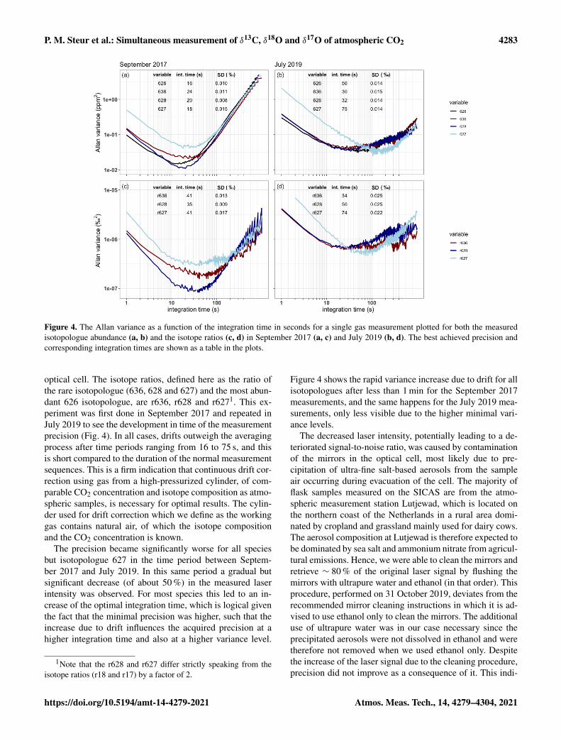
The gas inlet system, depicted in Fig. 3, is designed tomeasure discrete air samples in static mode, such that onecan quickly switch between measurements of different sam-ples. The system consists of Swagelok stainless steel tubingand connections and pneumatic valves. There are two inletports (11 and 14) which are connected to the sample crossat the heart of system (from now on indicated as inlet vol-ume), where a sample is collected at the target pressure of200±0.25 mbar before it is connected to the optical cell. Oneof the inlet ports (11) is connected to a 1/8” VICI multi-valve(Valco Instruments) with 15 potential positions for flask sam-ples or cylinders. The cylinders depicted in Fig. 3 will be de-fined in Sects. 2.2 and 3.2. When the VICI valve switchesfrom position, the volume between port 10 and 9 is flushedseven times with the sample gas to prevent memory effectsdue to the dead volume of the VICI valve. A sample gas isled into the inlet volume at reduced flow, as a critical ori-fice is placed right before the inlet valve, while another gasis being measured inside the optical cell. Since the closingand opening of the valves are controlled by the TDLWintelsoftware, it also controls the duration of the flow into the in-let volume. The target pressure is reached using input froma pressure sensor placed inside the inlet volume. After evac-uation of the optical cell (opening valve 22 and 23), the gasfrom the inlet volume can immediately be brought into theoptical cell (opening valve 19 and 23), thereby reducing thesample pressure to ∼ 50 mbar.
The gas handling procedures are different for measure-ments of air from cylinders or flasks. For the cylinders,single-stage pressure regulators are in use (Rotarex, modelSMT SI220), set at an outlet pressure of ∼ 600–1000 mbar(absolute). If measurements are started after more than 2 dof inactivity, the internal volume of the regulators is flushed10 times to prevent fractionation effects. To open and closethe flasks, we use a custom-built click-on electromotor valvesystem (Neubert et al., 2004), making it possible to open theflasks automatically before the measurement. Before openingthe flask, the volume between valve 9 and the closed flask isevacuated, so there is no need to flush extensively, and lesssample gas is lost. The actions described above are all steeredby a command program developed by Aerodyne ResearchInc. called the Switcher program. A bespoke script writing
https://doi.org/10.5194/amt-14-4279-2021 Atmos. Meas. Tech., 14, 4279–4304, 2021
4282 P. M. Steur et al.: Simultaneous measurement of δ13C, δ18O and δ17O of atmospheric CO2
Figure 2. Typical absorption spectrum, transmission spectrum and residual for laser 1 (a) for measurement of 627 and 626 and laser 2 (b)for measurement of 626, 628 and 636. The residuals show systematic deviations at the line positions. These deviations are primarily due tothe use of the Voigt line shape function in the spectral fitting model, rather than a more complex line shape function such as Hartmann–Tran.Careful analysis has shown that the use of the more convenient Voigt line shape function does not add noise, drift or calibration error asimplemented in the isotope analyzer.
Figure 3. Gas inlet system of the SICAS with one VICI multi-valve inlet port, connected to three high-pressure natural-air tanks and 12 freeports for samples. The includes an extra inlet port for the working gas, also a high-pressure natural-air tank.
program developed in FileMaker Pro enables us to quicklywrite scripts for measurement sequences and to directly linkthose measurements to an internal database.
2.2 Instrument performance
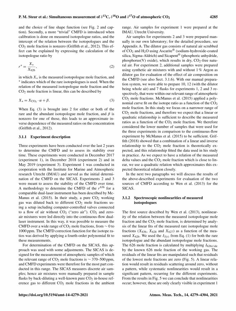
The SICAS measurement performance was evaluated by de-termining the Allan variance of the four measured isotopo-logue abundances and the three isotope ratios as a function ofmeasurement time on a single whole-air sample in the sealed
Atmos. Meas. Tech., 14, 4279–4304, 2021 https://doi.org/10.5194/amt-14-4279-2021
P. M. Steur et al.: Simultaneous measurement of δ13C, δ18O and δ17O of atmospheric CO2 4283
Figure 4. The Allan variance as a function of the integration time in seconds for a single gas measurement plotted for both the measuredisotopologue abundance (a, b) and the isotope ratios (c, d) in September 2017 (a, c) and July 2019 (b, d). The best achieved precision andcorresponding integration times are shown as a table in the plots.
optical cell. The isotope ratios, defined here as the ratio ofthe rare isotopologue (636, 628 and 627) and the most abun-dant 626 isotopologue, are r636, r628 and r6271. This ex-periment was first done in September 2017 and repeated inJuly 2019 to see the development in time of the measurementprecision (Fig. 4). In all cases, drifts outweigh the averagingprocess after time periods ranging from 16 to 75 s, and thisis short compared to the duration of the normal measurementsequences. This is a firm indication that continuous drift cor-rection using gas from a high-pressurized cylinder, of com-parable CO2 concentration and isotope composition as atmo-spheric samples, is necessary for optimal results. The cylin-der used for drift correction which we define as the workinggas contains natural air, of which the isotope compositionand the CO2 concentration is known.
The precision became significantly worse for all speciesbut isotopologue 627 in the time period between Septem-ber 2017 and July 2019. In this same period a gradual butsignificant decrease (of about 50 %) in the measured laserintensity was observed. For most species this led to an in-crease of the optimal integration time, which is logical giventhe fact that the minimal precision was higher, such that theincrease due to drift influences the acquired precision at ahigher integration time and also at a higher variance level.
1Note that the r628 and r627 differ strictly speaking from theisotope ratios (r18 and r17) by a factor of 2.
Figure 4 shows the rapid variance increase due to drift for allisotopologues after less than 1 min for the September 2017measurements, and the same happens for the July 2019 mea-surements, only less visible due to the higher minimal vari-ance levels.
The decreased laser intensity, potentially leading to a de-teriorated signal-to-noise ratio, was caused by contaminationof the mirrors in the optical cell, most likely due to pre-cipitation of ultra-fine salt-based aerosols from the sampleair occurring during evacuation of the cell. The majority offlask samples measured on the SICAS are from the atmo-spheric measurement station Lutjewad, which is located onthe northern coast of the Netherlands in a rural area domi-nated by cropland and grassland mainly used for dairy cows.The aerosol composition at Lutjewad is therefore expected tobe dominated by sea salt and ammonium nitrate from agricul-tural emissions. Hence, we were able to clean the mirrors andretrieve ∼ 80 % of the original laser signal by flushing themirrors with ultrapure water and ethanol (in that order). Thisprocedure, performed on 31 October 2019, deviates from therecommended mirror cleaning instructions in which it is ad-vised to use ethanol only to clean the mirrors. The additionaluse of ultrapure water was in our case necessary since theprecipitated aerosols were not dissolved in ethanol and weretherefore not removed when we used ethanol only. Despitethe increase of the laser signal due to the cleaning procedure,precision did not improve as a consequence of it. This indi-
https://doi.org/10.5194/amt-14-4279-2021 Atmos. Meas. Tech., 14, 4279–4304, 2021

4284 P. M. Steur et al.: Simultaneous measurement of δ13C, δ18O and δ17O of atmospheric CO2
Table 1. Relative standard deviations for n= 5 and n= 10 of un-corrected (uncor) and corrected (cor) isotope ratio sample measure-ments. Sample measurements were always bracketed by measure-ments of the working gas. Standard deviations of the uncorrectedmeasurements only use the sample measurements; standard devia-tions of the corrected measurements use drift-corrected (Eq. 1) sam-ple measurements using the working gas measurements.
All SD n= 5 n= 10
in ‰ uncor cor uncor cor
r636 0.04 0.020 0.06 0.025r628 0.05 0.021 0.10 0.029r627 0.06 0.018 0.18 0.03
cates that other, still unidentified, issues played a role in thedecrease of measurement precision.
To reduce short-term instrumental drift, all sample mea-surements needed to be alternated with measurements of theworking gas, as then the drift-corrected signal can be ex-pressed as
IS(t) =MS(t)
MWG(t), (1)
where M stands for measurement which can be either themeasured isotope ratio or isotopologue abundance, S standsfor sample, WG stands for working gas, t stands for timeof the sample gas measurement and I stands for the in-dex referring to the drift-corrected sample measurement,of either the isotope ratio or the isotopologue abundance.WG(t) is the measured working gas at time t derived fromthe time-dependent linear regression of the measurements ofthe working gas bracketing the sample gas measurement. Theeffectiveness of this drift correction method was tested for themeasured isotope ratios only. Although one of the tested cali-bration methods uses isotopologue abundances for the initialcalibration, the isotope composition is expressed as a deltavalue and will therefore eventually be calculated using iso-tope ratios (Sect. 3.3.3). The precision of the isotope ratioswill therefore always determine the measurement precision.
A tank was measured > 10 times alternately with theworking gas. The relative standard deviations were calcu-lated for n= 5 and n= 10, both with and without drift cor-rection (Table 1). It is expected that, if the drift correctionis effective, the standard deviations of the uncorrected val-ues are higher than the standard deviations of the correctedvalues. The drift correction is effective as the standard devi-ations of the corrected values are always lower than of theuncorrected values. Although the drift correction procedureis not perfect, as we see a small increase of the standarddeviation between n= 5 and n= 10 between 0.005 ‰ and0.012 ‰, we can still conclude that the drift correction willresult in a better repeatability of the isotope ratios.
Cross-contamination, being the dilution of a small volumeof the working gas in the sample aliquot that is being mea-sured, and vice versa, as described for a dual-inlet IRMS inMeijer et al. (2000), will occur in the SICAS due to the con-tinuous switching between sample and machine working gas.If cross-contamination is not corrected for, DI-IRMS mea-surement inaccuracy can occur when samples of a highly de-viating isotope composition are measured. On the SICAS,only atmospheric samples are measured that are of very sim-ilar isotope values. The CO2 mole fraction of the samplescan deviate quite strongly from the machine working gas,so effects of cross-contamination will have an influence onthe CO2 mole fraction in the optical cell. From experimen-tal data, we quantified the fraction of the preceding sam-ple that affects a sample measurement to be max 0.01 %.A sensitivity analysis was performed using this fraction andshowed that this is such a small amount that scale effects dueto cross-contamination are well below the precision foundin this study (for a detailed description of the analysis, seeAppendix E). If samples of CO2 concentrations outside therange of atmospheric samples are measured, it will be essen-tial to also take into account the surface adsorption effects ofthe aluminum cell which is known to adsorb CO2 (Leuen-berger et al., 2015). CO2 adsorption in the cell of the SICASwas clearly visible as a drop of measured CO2 concentrationwhen an atmospheric sample was let into the cell right afterthe cell was flushed with a CO2-free flush gas (hence strippedfrom CO2 molecules sticking to the cell surface).
3 Calibration experiments
3.1 The CO2 mole fraction dependency
The stable isotope composition of atmospheric CO2 is ex-pressed as a delta value on the VPDB (Vienna Pee DeeBelemnite) (13C)/VPDB-CO2 (17O and 18O) scales, whichare realized by producing CO2 gas (using phosphoric acidunder well-defined circumstances) from the IAEA-603 mar-ble primary reference material (successor to the now obsoleteNBS-19) (IAEA, 2016). A complication when compared toclassical DI-IRMS isotope measurements (or to optical mea-surements of pure CO2 for that matter) is that in the practiceof laser absorption spectroscopy the mole fraction of CO2in a gas affects the measured stable isotope ratios (and thusdelta values) of CO2. Quantification, let alone elimination ofthis CO2 mole fraction dependence (CMFD), is difficult (Mc-Manus et al., 2015), but two sources of CMFD were identi-fied by Wen et al. (2013) and related to different calibrationstrategies. In the first place, CMFD results from nonideal fit-ting of the absorption spectra, which will to some extent al-ways occur. Capturing the true absorption spectrum is verycomplicated, due to, among others, line broadening effects ofthe various components of the air, far wing overlap of distantbut strong absorptions, temperature and pressure variability
Atmos. Meas. Tech., 14, 4279–4304, 2021 https://doi.org/10.5194/amt-14-4279-2021
P. M. Steur et al.: Simultaneous measurement of δ13C, δ18O and δ17O of atmospheric CO2 4285
and the choice of line shape function (see Fig. 2 and cap-tion). Secondly, a more “trivial” CMFD is introduced whencalibration is done on measured isotopologue ratios, and theintercept of the relation between the isotopologues and theCO2 mole fraction is nonzero (Griffith et al., 2012). This ef-fect can be explained by expressing the calculation of theisotopologue ratio by
r∗ =X∗
X626, (2)
in which X∗ is the measured isotopologue mole fraction, and∗ indicates which of the rare isotopologues is used. When therelation of the measured isotopologue mole fraction and theCO2 mole fraction is linear, this can be described by
X∗ =XCO2 ·α+β. (3)
When Eq. (3) is brought into 2 for either or both of therare and the abundant isotopologue mole fraction, and β isnonzero for one of those, this leads to an approximate in-verse dependence of the measured ratios on the concentration(Griffith et al., 2012).
3.1.1 Experiment description
Three experiments have been conducted over the last 2 yearsto determine the CMFD and to assess its stability overtime. These experiments were conducted in December 2017(experiment 1), in December 2018 (experiment 2) and inMay 2019 (experiment 3). Experiment 1 was conducted incooperation with the Institute for Marine and Atmosphericresearch Utrecht (IMAU) and served as the initial determi-nation of the CMFD on the SICAS. Experiments 2 and 3were meant to assess the stability of the CMFD over time.A methodology to determine the CMFD of the r636 for acomparable dual-laser instrument has been described by Mc-Manus et al. (2015). In their study, a pure CO2 workinggas was diluted back to different CO2 mole fractions us-ing a setup including computer-controlled valves connectedto a flow of air without CO2 (“zero air”). CO2 and zero-air mixtures were led directly into the continuous-flow dual-laser instrument. In this way, it was possible to measure theCMFD over a wide range of CO2 mole fractions, from∼ 0 to1000 ppm. The CMFD correction function for the isotope ra-tios was derived by applying a fourth-order polynomial fit tothese measurements.
For determination of the CMFD on the SICAS, this ap-proach was used with some adjustments. The SICAS is de-signed for the measurement of atmospheric samples of whichthe relevant range of CO2 mole fractions is ∼ 370–500 ppm,and CMFD experiments were therefore for the most part con-ducted in this range. The SICAS measures discrete air sam-ples; hence air mixtures were manually prepared in sampleflasks by back-diluting a well-known pure CO2 in-house ref-erence gas to different CO2 mole fractions in the ambient
range. Air samples for experiment 1 were prepared at theIMAU, Utrecht University.
Air samples for experiments 2 and 3 were prepared man-ually in our own laboratory; for the detailed procedure, seeAppendix A. The dilutor gas consists of natural air scrubbedof CO2 and H2O using Ascarite® (sodium-hydroxide-coatedsilica, Sigma-Aldrich) and Sicapent® (phosphoric anhydride,phosphorus(V) oxide), which results in dry, CO2-free natu-ral air. For experiment 2, additional samples were preparedusing synthetic air mixtures with and without 1 % Argon asdilutor gas for evaluation of the effect of air composition onthe CMFD (see also Sect. 3.1.6). With our manual prepara-tion system, we were able to prepare 10, 12 (with the dilutorbeing whole air) and 7 flasks for experiments 1, 2 and 3 re-spectively, that were within our relevant range of atmosphericCO2 mole fractions. McManus et al. (2015) applied a poly-nomial curve fit on the isotope ratio as a function of the CO2mole fraction. In this study we focus on a narrower range ofCO2 mole fractions, and therefore we expect that a linear orquadratic relationship is sufficient to describe the measuredratios as a function of the CO2 mole fraction. We thereforeconsidered the lower number of samples that were used forthe three experiments in comparison to the continuous-flowexperiment by McManus et al. (2015) to be sufficient. Grif-fith (2018) showed that a combination of a linear and inverserelationship to the CO2 mole fraction is theoretically ex-pected, and this relationship fitted the data used in his studyin practice. As we expect to have a relation of the measureddelta values and the CO2 mole fraction which is close to lin-ear, we use a quadratic relation which approximates this ex-pected theoretical relation closely.
In the next two paragraphs we will discuss the results ofthe above-described experiments for evaluation of the twosources of CMFD according to Wen et al. (2013) for theSICAS.
3.1.2 Spectroscopic nonlinearities of measuredisotopologues
The first source described by Wen et al. (2013), nonlinear-ity of the relation between the measured isotopologue molefraction and the CO2 mole fraction, is determined by analy-sis of the linear fits of the measured rare isotopologue molefractions (X636, X628 and X627) as a function of the mea-sured X626. We used the IS(t) from Eq. (1) for both the rareisotopologue and the abundant isotopologue mole fractions.The 626 mole fraction is calculated by multiplying I626(t)dcby the known 626 mole fraction of the working gas. Theresiduals of the linear fits are manipulated such that residualsof the lowest mole fractions are zero (Fig. 5). A linear rela-tion would result in residuals scattering around zero, withouta pattern, while systematic nonlinearities would result in asignificant pattern, recurring for the different experiments.From the results in Fig. 5 we can conclude that nonlinearitiesoccur; however, these are only clearly visible in experiment 1
https://doi.org/10.5194/amt-14-4279-2021 Atmos. Meas. Tech., 14, 4279–4304, 2021
4286 P. M. Steur et al.: Simultaneous measurement of δ13C, δ18O and δ17O of atmospheric CO2
Figure 5. Residuals (expressed in ‰ relative to the measuredamount fraction) of the linear fit of the rare isotopologue abun-dances as a function of the X626 and the quadratic fit on the resid-uals. From top to bottom: experiment 1, experiment 2 and experi-ment 3. The colors red, dark blue and light blue are used for the iso-topologues 636, 628 and 627 respectively. Error bars are the com-bined standard deviations of the 626 and rare isotopologue measure-ments. Per isotopologue the R2 of the quadratic fit on the residualsis indicated in the tables on the right, as well as the maximum resid-ual (in ‰) on the linear fit of the rare isotopologue as a function ofthe X626.
for theX636 and theX627 isotopologue and to a lesser degreein experiment 2 for the X636 isotopologue. The maximumresiduals of both the X636 and the X627 are highest in exper-iment 1, which is also the experiment covering the highestrange of CO2 mole fractions. From these experiments we cantherefore conclude that nonlinearities of the measured rareisotopologue mole fractions and theX626 isotopologue occurbut are only significant if the range of CO2 mole fraction ishigher than 100 ppm. For the X628 we do not see significantnonlinearities, even if the CO2 mole fraction is much higherthan 100 ppm. The maximum residuals of the X628 are notinfluenced by the CO2 mole fraction, and we therefore con-clude that nonlinearities are below the level of detection inthese experiments.
3.1.3 Introduced dependency on measured delta values
The second source for CMFD, described by Wen et al.(2013), is the introduced dependency on measured isotoperatios if intercepts of the different isotopologues of the an-alyzer’s signal are nonzero, or as in our case for some ex-
Figure 6. Measured δ636 of three experiments; black points are ex-periment 1, red points are experiment 2 and green points are exper-iment 3.
periments, if different isotopologues of the analyzer’s signalare nonlinear in a different way. In this paragraph we lookinto the different possibilities to correct for the CMFD of themeasured deltas based on observations of the experimentsthat were described in the section above.
Isotope ratios are susceptible to instrumental drift, butdelta values are drift-corrected as the uncalibrated deltavalue δS is calculated by
δ∗S =
(r∗S(t)
r∗WG(t)− 1
), (4)
where S(t) and WG(t) stand for sample and working gasat the time of the sample measurement, respectively and∗ stands for the rare isotopologue of which the delta is cal-culated. The r∗WG(t) is calculated using the same methodasMWG(t) is calculated in Eq. (1). The CMFDs of the deltasare determined by conducting a linear fit on the measureddelta values as a function of the measured CO2 mole frac-tion.
The results for δ636 are shown in Fig. 6, and slopes of alldeltas and the standard errors of the slopes are shown in Ta-ble 2. Note that in some cases the standard error of the slopeis close to the slope itself, and it is therefore questionablewhether a significant CMFD is measured at all. As the CO2used for the different experiments was not of similar isotopecomposition, the δ636 measurements in Fig. 6 were normal-ized such that at the CO2 mole fraction of 400 ppm all ratiosare 1. Only the calculated slope is therefore of importancewhen considering the CMFD of the different experiments.From Table 2 it is clear that the δ636 shows the strongestCMFD. The results show that the CMFD varies for the threedifferent experiments for all measured deltas. Changing in-strumental conditions can be an explanation for this change
Atmos. Meas. Tech., 14, 4279–4304, 2021 https://doi.org/10.5194/amt-14-4279-2021
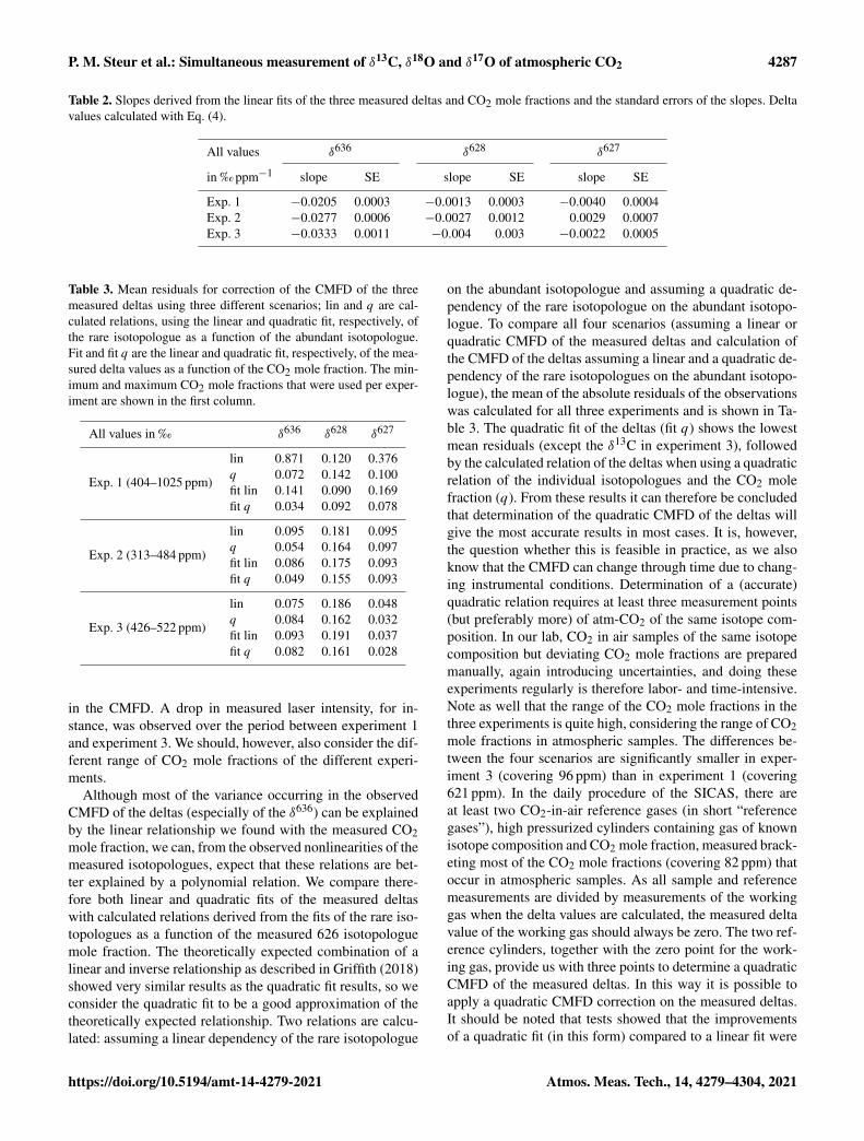
P. M. Steur et al.: Simultaneous measurement of δ13C, δ18O and δ17O of atmospheric CO2 4287
Table 2. Slopes derived from the linear fits of the three measured deltas and CO2 mole fractions and the standard errors of the slopes. Deltavalues calculated with Eq. (4).
All values δ636 δ628 δ627
in ‰ ppm−1 slope SE slope SE slope SE
Exp. 1 −0.0205 0.0003 −0.0013 0.0003 −0.0040 0.0004Exp. 2 −0.0277 0.0006 −0.0027 0.0012 0.0029 0.0007Exp. 3 −0.0333 0.0011 −0.004 0.003 −0.0022 0.0005
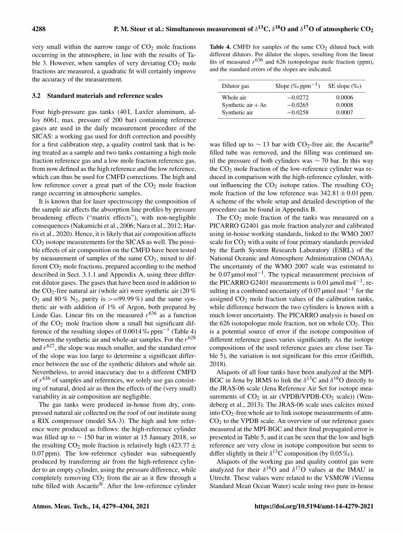
Table 3. Mean residuals for correction of the CMFD of the threemeasured deltas using three different scenarios; lin and q are cal-culated relations, using the linear and quadratic fit, respectively, ofthe rare isotopologue as a function of the abundant isotopologue.Fit and fit q are the linear and quadratic fit, respectively, of the mea-sured delta values as a function of the CO2 mole fraction. The min-imum and maximum CO2 mole fractions that were used per exper-iment are shown in the first column.
All values in ‰ δ636 δ628 δ627
Exp. 1 (404–1025 ppm)
lin 0.871 0.120 0.376q 0.072 0.142 0.100fit lin 0.141 0.090 0.169fit q 0.034 0.092 0.078
Exp. 2 (313–484 ppm)
lin 0.095 0.181 0.095q 0.054 0.164 0.097fit lin 0.086 0.175 0.093fit q 0.049 0.155 0.093
Exp. 3 (426–522 ppm)
lin 0.075 0.186 0.048q 0.084 0.162 0.032fit lin 0.093 0.191 0.037fit q 0.082 0.161 0.028
in the CMFD. A drop in measured laser intensity, for in-stance, was observed over the period between experiment 1and experiment 3. We should, however, also consider the dif-ferent range of CO2 mole fractions of the different experi-ments.
Although most of the variance occurring in the observedCMFD of the deltas (especially of the δ636) can be explainedby the linear relationship we found with the measured CO2mole fraction, we can, from the observed nonlinearities of themeasured isotopologues, expect that these relations are bet-ter explained by a polynomial relation. We compare there-fore both linear and quadratic fits of the measured deltaswith calculated relations derived from the fits of the rare iso-topologues as a function of the measured 626 isotopologuemole fraction. The theoretically expected combination of alinear and inverse relationship as described in Griffith (2018)showed very similar results as the quadratic fit results, so weconsider the quadratic fit to be a good approximation of thetheoretically expected relationship. Two relations are calcu-lated: assuming a linear dependency of the rare isotopologue
on the abundant isotopologue and assuming a quadratic de-pendency of the rare isotopologue on the abundant isotopo-logue. To compare all four scenarios (assuming a linear orquadratic CMFD of the measured deltas and calculation ofthe CMFD of the deltas assuming a linear and a quadratic de-pendency of the rare isotopologues on the abundant isotopo-logue), the mean of the absolute residuals of the observationswas calculated for all three experiments and is shown in Ta-ble 3. The quadratic fit of the deltas (fit q) shows the lowestmean residuals (except the δ13C in experiment 3), followedby the calculated relation of the deltas when using a quadraticrelation of the individual isotopologues and the CO2 molefraction (q). From these results it can therefore be concludedthat determination of the quadratic CMFD of the deltas willgive the most accurate results in most cases. It is, however,the question whether this is feasible in practice, as we alsoknow that the CMFD can change through time due to chang-ing instrumental conditions. Determination of a (accurate)quadratic relation requires at least three measurement points(but preferably more) of atm-CO2 of the same isotope com-position. In our lab, CO2 in air samples of the same isotopecomposition but deviating CO2 mole fractions are preparedmanually, again introducing uncertainties, and doing theseexperiments regularly is therefore labor- and time-intensive.Note as well that the range of the CO2 mole fractions in thethree experiments is quite high, considering the range of CO2mole fractions in atmospheric samples. The differences be-tween the four scenarios are significantly smaller in exper-iment 3 (covering 96 ppm) than in experiment 1 (covering621 ppm). In the daily procedure of the SICAS, there areat least two CO2-in-air reference gases (in short “referencegases”), high pressurized cylinders containing gas of knownisotope composition and CO2 mole fraction, measured brack-eting most of the CO2 mole fractions (covering 82 ppm) thatoccur in atmospheric samples. As all sample and referencemeasurements are divided by measurements of the workinggas when the delta values are calculated, the measured deltavalue of the working gas should always be zero. The two ref-erence cylinders, together with the zero point for the work-ing gas, provide us with three points to determine a quadraticCMFD of the measured deltas. In this way it is possible toapply a quadratic CMFD correction on the measured deltas.It should be noted that tests showed that the improvementsof a quadratic fit (in this form) compared to a linear fit were
https://doi.org/10.5194/amt-14-4279-2021 Atmos. Meas. Tech., 14, 4279–4304, 2021
4288 P. M. Steur et al.: Simultaneous measurement of δ13C, δ18O and δ17O of atmospheric CO2
very small within the narrow range of CO2 mole fractionsoccurring in the atmosphere, in line with the results of Ta-ble 3. However, when samples of very deviating CO2 molefractions are measured, a quadratic fit will certainly improvethe accuracy of the measurement.
3.2 Standard materials and reference scales
Four high-pressure gas tanks (40 L Luxfer aluminum, al-loy 6061, max. pressure of 200 bar) containing referencegases are used in the daily measurement procedure of theSICAS: a working gas used for drift correction and possiblyfor a first calibration step, a quality control tank that is be-ing treated as a sample and two tanks containing a high molefraction reference gas and a low mole fraction reference gas,from now defined as the high reference and the low reference,which can thus be used for CMFD corrections. The high andlow reference cover a great part of the CO2 mole fractionrange occurring in atmospheric samples.
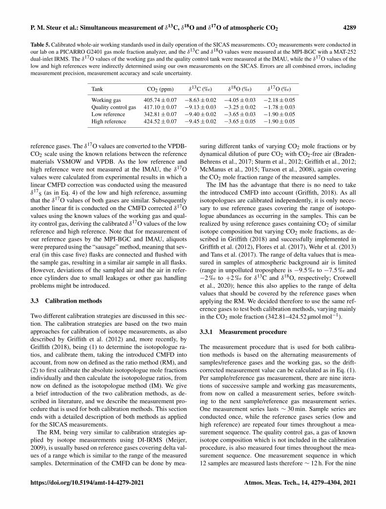
It is known that for laser spectroscopy the composition ofthe sample air affects the absorption line profiles by pressurebroadening effects (“matrix effects”), with non-negligibleconsequences (Nakamichi et al., 2006; Nara et al., 2012; Har-ris et al., 2020). Hence, it is likely that air composition affectsCO2 isotope measurements for the SICAS as well. The possi-ble effects of air composition on the CMFD have been testedby measurement of samples of the same CO2, mixed to dif-ferent CO2 mole fractions, prepared according to the methoddescribed in Sect. 3.1.1 and Appendix A, using three differ-ent dilutor gases. The gases that have been used in addition tothe CO2-free natural air (whole air) were synthetic air (20 %O2 and 80 % N2, purity is >=99.99 %) and the same syn-thetic air with addition of 1% of Argon, both prepared byLinde Gas. Linear fits on the measured r636 as a functionof the CO2 mole fraction show a small but significant dif-ference of the resulting slopes of 0.0014 ‰ ppm−1 (Table 4)between the synthetic air and whole-air samples. For the r628
and r627, the slope was much smaller, and the standard errorof the slope was too large to determine a significant differ-ence between the use of the synthetic dilutors and whole air.Nevertheless, to avoid inaccuracy due to a different CMFDof r636 of samples and references, we solely use gas consist-ing of natural, dried air as then the effects of the (very small)variability in air composition are negligible.
The gas tanks were produced in-house from dry, com-pressed natural air collected on the roof of our institute usinga RIX compressor (model SA-3). The high and low refer-ence were produced as follows: the high-reference cylinderwas filled up to ∼ 150 bar in winter at 15 January 2018, sothe resulting CO2 mole fraction is relatively high (423.77±0.07 ppm). The low-reference cylinder was subsequentlyproduced by transferring air from the high-reference cylin-der to an empty cylinder, using the pressure difference, whilecompletely removing CO2 from the air as it flew through atube filled with Ascarite®. After the low-reference cylinder
Table 4. CMFD for samples of the same CO2 diluted back withdifferent dilutors. Per dilutor the slopes, resulting from the linearfits of measured r636 and 626 isotopologue mole fraction (ppm),and the standard errors of the slopes are indicated.
Dilutor gas Slope (‰ ppm−1) SE slope (‰)
Whole air −0.0272 0.0006Synthetic air+Ar. −0.0265 0.0008Synthetic air −0.0258 0.0007
was filled up to ∼ 13 bar with CO2-free air, the Ascarite®
filled tube was removed, and the filling was continued un-til the pressure of both cylinders was ∼ 70 bar. In this waythe CO2 mole fraction of the low-reference cylinder was re-duced in comparison with the high-reference cylinder, with-out influencing the CO2 isotope ratios. The resulting CO2mole fraction of the low reference was 342.81± 0.01 ppm.A scheme of the whole setup and detailed description of theprocedure can be found in Appendix B.
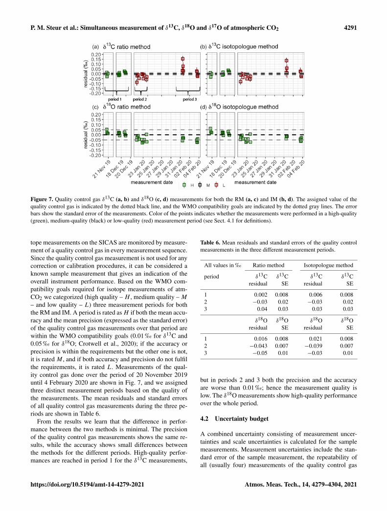
The CO2 mole fraction of the tanks was measured on aPICARRO G2401 gas mole fraction analyzer and calibratedusing in-house working standards, linked to the WMO 2007scale for CO2 with a suite of four primary standards providedby the Earth System Research Laboratory (ESRL) of theNational Oceanic and Atmosphere Administration (NOAA).The uncertainty of the WMO 2007 scale was estimated tobe 0.07 µmol mol−1. The typical measurement precision ofthe PICARRO G2401 measurements is 0.01 µmol mol−1, re-sulting in a combined uncertainty of 0.07 µmol mol−1 for theassigned CO2 mole fraction values of the calibration tanks,while difference between the two cylinders is known with amuch lower uncertainty. The PICARRO analysis is based onthe 626 isotopologue mole fraction, not on whole CO2. Thisis a potential source of error if the isotope composition ofdifferent reference gases varies significantly. As the isotopecompositions of the used reference gases are close (see Ta-ble 5), the variation is not significant for this error (Griffith,2018).
Aliquots of all four tanks have been analyzed at the MPI-BGC in Jena by IRMS to link the δ13C and δ18O directly tothe JRAS-06 scale (Jena Reference Air Set for isotope mea-surements of CO2 in air (VPDB/VPDB-CO2 scale)) (Wen-deberg et al., 2013). The JRAS-06 scale uses calcites mixedinto CO2-free whole air to link isotope measurements of atm-CO2 to the VPDB scale. An overview of our reference gasesmeasured at the MPI-BGC and their final propagated error ispresented in Table 5, and it can be seen that the low and highreference are very close in isotope composition but seem todiffer slightly in their δ13C composition (by 0.05 ‰).
Aliquots of the working gas and quality control gas wereanalyzed for their δ18O and δ17O values at the IMAU inUtrecht. These values were related to the VSMOW (ViennaStandard Mean Ocean Water) scale using two pure in-house
Atmos. Meas. Tech., 14, 4279–4304, 2021 https://doi.org/10.5194/amt-14-4279-2021
P. M. Steur et al.: Simultaneous measurement of δ13C, δ18O and δ17O of atmospheric CO2 4289
Table 5. Calibrated whole-air working standards used in daily operation of the SICAS measurements. CO2 measurements were conducted inour lab on a PICARRO G2401 gas mole fraction analyzer, and the δ13C and δ18O values were measured at the MPI-BGC with a MAT-252dual-inlet IRMS. The δ17O values of the working gas and the quality control tank were measured at the IMAU, while the δ17O values of thelow and high references were indirectly determined using our own measurements on the SICAS. Errors are all combined errors, includingmeasurement precision, measurement accuracy and scale uncertainty.
Tank CO2 (ppm) δ13C (‰) δ18O (‰) δ17O (‰)
Working gas 405.74± 0.07 −8.63± 0.02 −4.05± 0.03 −2.18± 0.05Quality control gas 417.10± 0.07 −9.13± 0.03 −3.25± 0.02 −1.78± 0.03Low reference 342.81± 0.07 −9.40± 0.02 −3.65± 0.03 −1.90± 0.05High reference 424.52± 0.07 −9.45± 0.02 −3.65± 0.05 −1.90± 0.05
reference gases. The δ17O values are converted to the VPDB-CO2 scale using the known relations between the referencematerials VSMOW and VPDB. As the low reference andhigh reference were not measured at the IMAU, the δ17Ovalues were calculated from experimental results in which alinear CMFD correction was conducted using the measuredδ17
S (as in Eq. 4) of the low and high reference, assumingthat the δ17O values of both gases are similar. Subsequentlyanother linear fit is conducted on the CMFD corrected δ17Ovalues using the known values of the working gas and qual-ity control gas, deriving the calibrated δ17O values of the lowreference and high reference. Note that for measurement ofour reference gases by the MPI-BGC and IMAU, aliquotswere prepared using the “sausage” method, meaning that sev-eral (in this case five) flasks are connected and flushed withthe sample gas, resulting in a similar air sample in all flasks.However, deviations of the sampled air and the air in refer-ence cylinders due to small leakages or other gas handlingproblems might be introduced.
3.3 Calibration methods
Two different calibration strategies are discussed in this sec-tion. The calibration strategies are based on the two mainapproaches for calibration of isotope measurements, as alsodescribed by Griffith et al. (2012) and, more recently, byGriffith (2018), being (1) to determine the isotopologue ra-tios, and calibrate them, taking the introduced CMFD intoaccount, from now on defined as the ratio method (RM), and(2) to first calibrate the absolute isotopologue mole fractionsindividually and then calculate the isotopologue ratios, fromnow on defined as the isotopologue method (IM). We givea brief introduction of the two calibration methods, as de-scribed in literature, and we describe the measurement pro-cedure that is used for both calibration methods. This sectionends with a detailed description of both methods as appliedfor the SICAS measurements.
The RM, being very similar to calibration strategies ap-plied by isotope measurements using DI-IRMS (Meijer,2009), is usually based on reference gases covering delta val-ues of a range which is similar to the range of the measuredsamples. Determination of the CMFD can be done by mea-
suring different tanks of varying CO2 mole fractions or bydynamical dilution of pure CO2 with CO2-free air (Braden-Behrens et al., 2017; Sturm et al., 2012; Griffith et al., 2012;McManus et al., 2015; Tuzson et al., 2008), again coveringthe CO2 mole fraction range of the measured samples.
The IM has the advantage that there is no need to takethe introduced CMFD into account (Griffith, 2018). As allisotopologues are calibrated independently, it is only neces-sary to use reference gases covering the range of isotopo-logue abundances as occurring in the samples. This can berealized by using reference gases containing CO2 of similarisotope composition but varying CO2 mole fractions, as de-scribed in Griffith (2018) and successfully implemented inGriffith et al. (2012), Flores et al. (2017), Wehr et al. (2013)and Tans et al. (2017). The range of delta values that is mea-sured in samples of atmospheric background air is limited(range in unpolluted troposphere is −9.5 ‰ to −7.5 ‰ and−2 ‰ to +2 ‰ for δ13C and δ18O, respectively; Crotwellet al., 2020); hence this also applies to the range of deltavalues that should be covered by the reference gases whenapplying the RM. We decided therefore to use the same ref-erence gases to test both calibration methods, varying mainlyin the CO2 mole fraction (342.81–424.52 µmol mol−1).
3.3.1 Measurement procedure
The measurement procedure that is used for both calibra-tion methods is based on the alternating measurements ofsamples/reference gases and the working gas, so the drift-corrected measurement value can be calculated as in Eq. (1).Per sample/reference gas measurement, there are nine itera-tions of successive sample and working gas measurements,from now on called a measurement series, before switch-ing to the next sample/reference gas measurement series.One measurement series lasts ∼ 30 min. Sample series areconducted once, while the reference gases series (low andhigh reference) are repeated four times throughout a mea-surement sequence. The quality control gas, a gas of knownisotope composition which is not included in the calibrationprocedure, is also measured four times throughout the mea-surement sequence. One measurement sequence in which12 samples are measured lasts therefore ∼ 12 h. For the nine
https://doi.org/10.5194/amt-14-4279-2021 Atmos. Meas. Tech., 14, 4279–4304, 2021

4290 P. M. Steur et al.: Simultaneous measurement of δ13C, δ18O and δ17O of atmospheric CO2
measurement values of each measurement series, outliers aredetermined using the outlier identification method for verysmall samples by Rousseeuw and Verboven (2002), and themean values of the measurement series are calculated.
3.3.2 Ratio method
In the RM, measured isotopologue mole fractions are usedfor the estimation of isotope ratios (Eq. 1), which are cali-brated to the international VPDB-CO2 scale by measurementof several in-house CO2-in-air references within the samemeasurement sequence. The working gas is used both fordrift correction and a first calibration step, and the uncali-brated delta value δS is calculated by
δ∗S =
(r∗Sr∗WG− 1
), (5)
where S and WG stand for sample and working gas respec-tively. The calibrated δ13C, δ18O and δ17O based on theworking gas that is used are then derived by
δSCal = (1+ δWG) · δS+ δWG, (6)
in which δWG is the known delta value of the working gas onthe VPDB-CO2 scale.
Up to this point, the procedures are more or less identicalto those for IRMS measurements (but without the ion cor-rection and N2O correction unnecessary here). CMFD cor-rection is specific for laser absorption spectroscopy and iscrucial (as can be concluded from Sect. 3.1.3) to derive ac-curate measurement results when calibration is done usingthe isotope ratios. We developed a calibration method basedon the idea that including the measurement of two referencegases covering the CO2 mole fraction range of the measuredsamples (in our case the low- and high-reference gas) en-ables the correction of the measured isotope ratios. Thesetwo reference gases are measured several times throughoutthe measurement sequence and a quadratic fit of the mean ofthe residuals (measured δSCal – assigned δVPDB), includingthe residual of zero for the (hypothetical) working gas mea-surement, as a function of the CO2 mole fraction is done, sothe following calibration formula can then be determined:
δVPDB = δSCal−(
[CO2]2· a+ [CO2] · b+ c
), (7)
in which a and b are the second- and first-order coefficientsrespectively, c is the intercept of the quadratic fit of the resid-uals and the CO2 mole fractions of the two reference gases,[CO2] is the measured CO2 mole fraction and δVPDB is thecalibrated δ value on the VPDB scale.
3.3.3 Isotopologue method
The IM as described by Flores et al. (2017) following meth-ods earlier described by Griffith et al. (2012) will be brieflyexplained here for clarity, before explaining the applicationof the IM on the SICAS. Basically, the method treats the CO2isotopologues as if they were independent species, calibratestheir mixing ratios individually and only then combines theresults to build isotope ratios and delta values. The mole frac-tions (X) of the four most abundant isotopologues of a mea-sured CO2 sample are determined using a suite (in our casethe working gas and the high- and low-reference gas) of ref-erences gases with known CO2 mole fractions and isotopecompositions. The CO2 mole fractions are ideally chosensuch that normally occurring CO2 mole fractions in atmo-spheric air are bracketed by the two reference gases. The low-and high-reference gases cover the range between 324.81 and424.52 ppm, meaning that this method is only valid for sam-ples within that range of CO2 concentrations. The actual (orassigned) mole fractions (Xa) of the four most abundant iso-topologues of the reference gases can be calculated using cal-culations 1–11 in Flores et al. (2017), which are listed in Ap-pendix B. Although the nonlinearity of isotopologues as afunction of the absolute CO2 mole fraction has not been in-vestigated in this study, it is very likely that nonlinearitiesoccur, according to the results discussed in Sect. 3.1.2. Thebroad range of CO2 mole fractions that are covered by thereference gases, together with a hypothetical measurementof the working gas (of which the normalized isotopologueabundance will always be 1), enable us to do a quadratic fitof the measured isotopologue abundance as a function of theassigned isotopologue mole fractions, by
Xa =X2m · c+Xm · d + e, (8)
in which c and d are the second- and first-order coefficients,respectively, and e is the intercept of the quadratic fit of Xmas a function of Xa of the reference gases. The resulting Xavalues are used to calculate the isotope composition usingcalculation 1–11 in Appendix B. The introduced CMFD dueto calibration on measured isotope ratios will not occur withthis method, and a CMFD correction is therefore not neces-sary to yield accurate results.
A complete overview of all calculation steps of both theRM and IM can be found in Appendix C.
4 Results and discussion
4.1 Monitoring measurement quality and comparisonof calibration methods of δ13C and δ18O
To capture the very small signals in time series of the isotopecomposition of atm-CO2, it is crucial to keep track of theinstrument’s performance over the course of longer measure-ment periods. Variations in precision and accuracy of the iso-
Atmos. Meas. Tech., 14, 4279–4304, 2021 https://doi.org/10.5194/amt-14-4279-2021
P. M. Steur et al.: Simultaneous measurement of δ13C, δ18O and δ17O of atmospheric CO2 4291
Figure 7. Quality control gas δ13C (a, b) and δ18O (c, d) measurements for both the RM (a, c) and IM (b, d). The assigned value of thequality control gas is indicated by the dotted black line, and the WMO compatibility goals are indicated by the dotted gray lines. The errorbars show the standard error of the measurements. Color of the points indicates whether the measurements were performed in a high-quality(green), medium-quality (black) or low-quality (red) measurement period (see Sect. 4.1 for definitions).
tope measurements on the SICAS are monitored by measure-ment of a quality control gas in every measurement sequence.Since the quality control gas measurement is not used for anycorrection or calibration procedures, it can be considered aknown sample measurement that gives an indication of theoverall instrument performance. Based on the WMO com-patibility goals required for isotope measurements of atm-CO2 we categorized (high quality – H , medium quality – M– and low quality – L) three measurement periods for boththe RM and IM. A period is rated asH if both the mean accu-racy and the mean precision (expressed as the standard error)of the quality control gas measurements over that period arewithin the WMO compatibility goals (0.01 ‰ for δ13C and0.05 ‰ for δ18O; Crotwell et al., 2020); if the accuracy orprecision is within the requirements but the other one is not,it is rated M , and if both accuracy and precision do not fulfilthe requirements, it is rated L. Measurements of the qual-ity control gas done over the period of 20 November 2019until 4 February 2020 are shown in Fig. 7, and we assignedthree distinct measurement periods based on the quality ofthe measurements. The mean residuals and standard errorsof all quality control gas measurements during the three pe-riods are shown in Table 6.
From the results we learn that the difference in perfor-mance between the two methods is minimal. The precisionof the quality control gas measurements shows the same re-sults, while the accuracy shows small differences betweenthe methods for the different periods. High-quality perfor-mances are reached in period 1 for the δ13C measurements,
Table 6. Mean residuals and standard errors of the quality controlmeasurements in the three different measurement periods.
All values in ‰ Ratio method Isotopologue method
period δ13C δ13C δ13C δ13Cresidual SE residual SE
1 0.002 0.008 0.006 0.0082 −0.03 0.02 −0.03 0.023 0.04 0.03 0.03 0.03
δ18O δ18O δ18O δ18Oresidual SE residual SE
1 0.016 0.008 0.021 0.0082 −0.043 0.007 −0.039 0.0073 −0.05 0.01 −0.03 0.01
but in periods 2 and 3 both the precision and the accuracyare worse than 0.01 ‰; hence the measurement quality islow. The δ18O measurements show high-quality performanceover the whole period.
4.2 Uncertainty budget
A combined uncertainty consisting of measurement uncer-tainties and scale uncertainties is calculated for the samplemeasurements. Measurement uncertainties include the stan-dard error of the sample measurement, the repeatability ofall (usually four) measurements of the quality control gas
https://doi.org/10.5194/amt-14-4279-2021 Atmos. Meas. Tech., 14, 4279–4304, 2021
4292 P. M. Steur et al.: Simultaneous measurement of δ13C, δ18O and δ17O of atmospheric CO2
throughout the measurement sequence and the residual of themean of the quality control gas measurements from the as-signed value. The measurement uncertainties will thereforevary with each measurement/measurement sequence. We ob-serve a high repeatability in all sequences included in theanalysis of Fig. 7 (eight in total), with standard errors rang-ing between 0.008 ‰ and 0.03 ‰ and a mean of 0.02 ‰ forδ13C and standard errors ranging between 0.007 ‰ and0.01 ‰ and a mean of 0.008 ‰ for δ18O, for both meth-ods. The residuals in these sequences show a higher contri-bution to the combined uncertainty and a small differencebetween the two calibration methods. The absolute residualsof the RM range between 0.002 ‰ and 0.04 ‰ with a meanof 0.024 ‰ for δ13C and between 0.016 ‰ and 0.05 ‰ with amean of 0.04 ‰ for δ18O. For the IM the residuals range be-tween 0.006 ‰ and 0.03 ‰ with a mean of 0.02 ‰ for δ13Cand between 0.012 ‰ and 0.04 ‰ with a mean of 0.03 ‰ forδ18O. Hence, the RM shows slightly higher contributions tothe combined uncertainty as a result of the accuracy of thequality control gas measurements.
The scale uncertainties, which are fixed for all measure-ment sequences in which the working gas, low reference andhigh reference are used for the sample calibration, were sim-ulated using the Monte Carlo method. Input values were gen-erated by choosing random numbers of normal distributionwith the assigned value and uncertainty as in Table 5, be-ing the mean and the standard deviation around the mean,respectively. As the RM and IM follow different calibrationschemes, the Monte Carlo simulations are discussed sepa-rately; for the RM the scale uncertainties of the assigned deltavalues result in an uncertainty in the calculated residualswhich are quadratically fitted against the measured CO2 molefraction. The average uncertainties in the calibrated delta val-ues of the five simulations are 0.03 ‰ and 0.05 ‰ for δ13Cand δ18O, respectively.
Besides the uncertainties introduced by the scale uncer-tainties of the delta values, the calibrated measurements ofthe IM are also affected by the scale uncertainties of the CO2mole fractions. Both the uncertainties in the delta values andin the CO2 mole fractions affect the calculated assigned iso-topologue abundances, which are quadratically fitted againstthe measured isotopologue abundances. The uncertainties inthe assigned delta values result in average uncertainties of0.03 ‰ and 0.06 ‰ for δ13C and δ18O, respectively. The un-certainties in the assigned CO2 mole fractions result in un-certainties of 0.005 ‰ and 0.018 ‰ for δ13C and δ18O, re-spectively, and are small compared to the uncertainties of theassigned delta values.
Reducing the combined uncertainty of the δ13C and δ18Omeasurements of the SICAS will be most effective by deter-mining the isotope composition of the reference gases with alower uncertainty on the VPDB-CO2 scale.
4.3 Intercomparison flask measurements
To test the accuracy of SICAS flask measurements over awide range of CO2 mixing ratios, as well as testing thelab compatibility of the SICAS measurements, we measuredflask samples that are part of an ongoing lab intercomparisonof atmospheric trace gas measurements including the δ13Cand δ18O of CO2 (Levin et al., 2004). Since 2002, the sausageflask intercomparison program (from now on defined as ICP)has provided aliquots of three high-pressure cylinders con-taining natural air covering a CO2 mixing ratio range of 340–450 µmol mol−1 every 2 to 3 months (occasionally longer pe-riods). Participating laboratories send six flasks to the ICOS-CAL lab in Jena where these are filled with air from the threecylinders (two flasks per cylinder) with the sausage method.The ICP provides therefore the opportunity to compare flaskmeasurements on the SICAS with IRMS flask measurementsof the MPI-BGC and other groups. We measured sausage se-ries 90–94, which were filled between April 2018 and Jan-uary 2020, and calibrated the isotope measurements bothwith the RM and the IM. SICAS measurements took place inthe period from December 2019 to April 2020, with the con-sequence that the storage time of the flasks varies between3 and 20 months. To place these results in the context of inter-comparison results of well-established isotope and measure-ment laboratories, the ICP results of the Earth System Re-search Laboratory of the National Oceanic and AtmosphericAdministration (NOAA) (Trolier et al., 1996) were also com-pared to the MPI-BGC results for the same sausage series.
The lab intercomparison is presented in the usual way: themean and standard deviation of the differences between ourSICAS δ13C and δ18O results (both RM and IM calibrated)and the MPI-BGC ones are shown in Table 7, along withthe NOAA-MPI-BGC differences. The mean values of thedifferences for the SICAS RM and NOAA results are bothbelow 0.01 ‰, while the standard deviations of the differ-ences are 0.05 ‰ and 0.07 ‰, respectively. The SICAS re-sults calibrated with the IM show an offset with MPI-BGCof −0.013 ‰ and a standard deviation of the differences of0.07 ‰. We can therefore conclude that the differences inperformance between the RM and the IM are minimal, andboth methods show comparable results for the measured dif-ferences between MPI-BGC as for the differences betweenthe NOAA and the MPI-BGC.
When we compare the δ18O measurements, we find thatthe SICAS results are consequently significantly more de-pleted with an average difference of −0.4 ‰ compared tothe MPI-BGC results and that the differences vary stronglywith a standard deviation of 0.16 ‰. δ18O results of the ICPprogram show in general a larger scatter among the labs thanδ13C results (Levin et al., 2004), as is also visible in Table 7for the NOAA-MPI-BGC differences. The differences be-tween the SICAS- and the MPI-BGC results, however, arefar larger than those (or than in fact all differences in theICP program). The reason for this signal being too depleted
Atmos. Meas. Tech., 14, 4279–4304, 2021 https://doi.org/10.5194/amt-14-4279-2021

P. M. Steur et al.: Simultaneous measurement of δ13C, δ18O and δ17O of atmospheric CO2 4293
Table 7. Lab intercomparison of ICP sausage 90–94 results, onlyincluding data points within the CO2 mole fraction range of theused calibration tanks (342.81–424.52 µmol mol−1). Differencesbetween the SICAS, of both calibration methods, as well as theNOAA IRMS results and the MPI-BGC IRMS results are shown.The mean difference as well as the standard deviation of the differ-ences of the δ13C and δ18O are shown.
δ13C δ18O
All values in ‰ Mean SD Mean SD
SICAS – MPI-BGC RM 0.009 0.05 −0.4 0.16IM −0.013 0.07 −0.4 0.16
NOAA – MPI-BGC −0.007 0.07 0.130 0.08
is presumably equilibration of CO2 with water molecules onthe glass surface inside the CIO-type sample flasks duringstorage. Earlier (unpublished) results from our CO2 extrac-tion system indicated that the water content of our dried at-mospheric air samples increased as a function of time in-side the flasks. Our atmospheric samples are stored at atmo-spheric pressure or lower (down to∼ 800 mbar) when part ofthe sample has been consumed by different measurement de-vices. The CIO flasks are sealed with two Louwers–Hapertvalves and Viton O-rings of which it is known that perme-ation of water vapor (as well as other gases) occurs over time(Sturm et al., 2004). Both the pressure gradient and the watervapor gradient between the lab atmosphere and the dry sam-ple air inside the flask lead to permeation of water moleculesthrough the valve seals. To check this hypothesis, an exper-iment was conducted in which CIO flasks were filled withquality control gas and were measured the same day of thefilling procedure and 1 week and 3 months later (see Table 8).The results show no significant change in the δ13C, while forthe δ18O there is a strong depletion of the flask measurementsafter 3 months, deviating more than−0.2 ‰ in comparison tothe cylinder measurements. After 1 week there is no changein the δ18O, indicating that depletion of the δ18O in the CIOflasks occurs over longer time periods. As the flasks fromthe ICP were measured at the SICAS after relatively longstorage times, sometimes almost 2 years, this is likely the ex-planation of the values being too depleted in comparison tothe MPI-BGC results. A depletion twice as small as for δ18Ois observed in the δ17O values, as one would expect for iso-topic exchange with water. Further investigations about thechanging oxygen isotope signal in CIO-sample flasks are be-ing conducted with the aim to be able to make reliable assess-ments of the quality of δ18O and δ17O flask measurements onthe SICAS.
To check the performance of the SICAS for both the IMand RM over the wide CO2 range that is covered by the ICPsausage samples, the differences between the MPI-BGC andthe SICAS results are plotted in Fig. 8 against the measuredCO2 mole fraction. Shown is that for both methods the high-
Figure 8. Results of the intercomparison of δ13C measurements onthe SICAS and on the IRMS facility at the MPI-BGC for both theRM (a) and IM (b). The MPI-BGC results were subtracted fromthe SICAS results, and the error bars show the combined uncer-tainty of the SICAS measurements. The dotted gray lines show the0.03 ‰ range of residuals. Red data points are outside of the CO2mole fraction range of the reference gases.
est differences are seen at the higher end of the CO2 molefraction above 425 ppm and therefore far out of the range thatis covered by the high and low references (∼ 343–425 ppm).Extrapolation of the calibration methods outside the CO2mole fraction range of the reference gases yields worse com-patibility with MPI-BGC, possibly due to the nonlinear char-acter of both the isotopologue CO2 dependency and the ratioCO2 dependency. It should therefore be concluded that, toachieve highly accurate results of isotope measurements overthe whole range of CO2 mole fractions found in atmosphericsamples, the range covered by the reference gases would ide-ally be changed to∼ 380–450 ppm. The results of the IM areslightly better in the CO2 range above 425 ppm; specifically,the point closest to 440 ppm shows a significantly smallerresidual (∼ 0.1 ‰ less) than the RM. The better result ofextrapolation of the determined calibration curves for theIM method could be due to the lesser degree of nonlinear-ity of the measured isotopologue abundances as a functionof the assigned isotopologue abundances, in comparison tothe nonlinearity of the measured isotope ratios as a functionof the CO2 mole fraction. More points in this higher rangeare needed, however, to draw any further conclusions on thismatter.
4.4 Potential of SICAS 117O measurements foratmospheric research
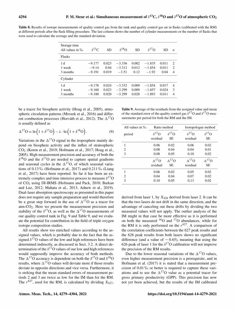
With the direct measurement of δ17O in addition to δ18O(triple oxygen isotope composition) of atm-CO2, the δ17Oexcess (117O) can be calculated. 117O measurements can
https://doi.org/10.5194/amt-14-4279-2021 Atmos. Meas. Tech., 14, 4279–4304, 2021
4294 P. M. Steur et al.: Simultaneous measurement of δ13C, δ18O and δ17O of atmospheric CO2
Table 8. Results of isotope measurements of quality control gas from the tank and quality control gas air in flasks (calibrated with the RM)at different periods after the flask filling procedure. The last column shows the number of cylinder measurements or the number of flasks thatwere used to calculate the average and the standard deviation.
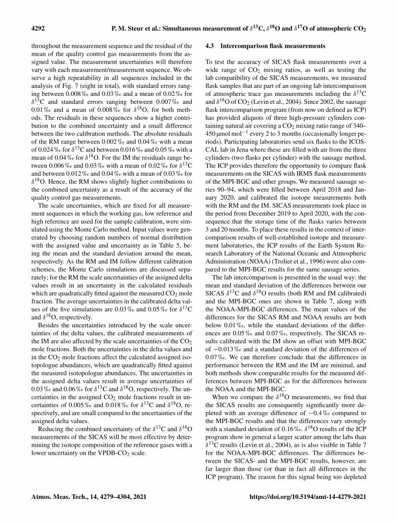
Storage timeAll values in ‰ δ13C SD δ18O SD δ17O SD n
Flasks
1 d −9.177 0.023 −3.336 0.002 −1.835 0.011 21 week −9.14 0.04 −3.312 0.012 −1.854 0.011 23 months −9.191 0.019 −3.51 0.12 −1.92 0.04 4
Cylinder
1 d −9.178 0.024 −3.332 0.009 −1.854 0.017 41 week −9.160 0.023 −3.299 0.009 −1.857 0.024 33 months −9.180 0.020 −3.299 0.028 −1.893 0.011 4
be a tracer for biosphere activity (Hoag et al., 2005), atmo-spheric circulation patterns (Mrozek et al., 2016) and differ-ent combustion processes (Horváth et al., 2012). The 117Ois usually defined as
117O= ln(
1+ δ17O)− λ · ln
(1+ δ18O
). (9)
Variations in the 117O signal in the troposphere mainly de-pend on biosphere activity and the influx of stratosphericCO2 (Koren et al., 2019; Hofmann et al., 2017; Hoag et al.,2005). High measurement precision and accuracy of both theδ18O and the δ17O are needed to capture spatial gradientsand seasonal cycles in the 117O, of which seasonal varia-tions of 0.13 ‰ (Hofmann et al., 2017) and 0.211 ‰ (Lianget al., 2017) have been reported. So far it has been an ex-tremely complex and time intensive process to measure δ17Oof CO2 using DI-IRMS (Hofmann and Pack, 2010; Barkanand Luz, 2012; Mahata et al., 2013; Adnew et al., 2019).Dual-laser absorption spectroscopy as presented in this paperdoes not require any sample preparation and would thereforebe a great step forward in the use of 117O as a tracer foratm-CO2. Here we present the measurement precision andstability of the δ17O, as well as the 117O measurements ofour quality control tank in Fig. 9 and Table 9, and we evalu-ate the potential for contribution in the field of triple oxygenisotope composition studies.
All results show too enriched values according to the as-signed values, which is probably due to the fact that the as-signed δ17O values of the low and high references have beendetermined indirectly, as discussed in Sect. 3.2. A direct de-termination of the δ17O values of our low and high referenceswould supposedly improve the accuracy of both methods.The 117O accuracy is dependent on both the δ17O and δ18Oresults, where 117O values will deviate more if those resultsdeviate in opposite directions and vice versa. Furthermore, itis striking that the mean standard errors of measurement pe-riods 2 and 3 are twice as low for the IM than for the RM.The r627, used for the RM, is calculated by dividing X627,
Table 9. Average of the residuals from the assigned value and meanof the standard error of the quality control gas δ17O and δ17O mea-surements per period for both the RM and the IM.
All values in ‰ Ratio method Isotopologue method
period δ17O δ17O δ17O δ17Oresidual SE residual SE
1 0.06 0.02 0.06 0.022 0.08 0.04 0.04 0.013 0.08 0.05 0.10 0.02
117O 117O 117O 117Oresidual SE residual SE
1 0.06 0.02 0.05 0.022 0.04 0.04 0.07 0.023 0.10 0.05 0.13 0.02
derived from laser 1, by X626 derived from laser 2. It can bethat the two lasers do not drift in the same direction, and theadvantage of canceling out these drifts by dividing the twomeasured values will not apply. The outlier analysis of theIM might in that case be more effective as it is performedon both the measured 16O and 17O abundances, while forthe RM it is only performed on the r627. A comparison ofthe correlation coefficients between the 627 peak results andthe 626 peak results from both lasers shows no significantdifference (and a value of ∼ 0.65), meaning that using the626 peak of laser 1 for the δ17O calibration will not improvethe precision of the RM results.
Due to the lower seasonal variations of the 117O values,even higher measurement precision is a prerequisite, and inHofmann et al. (2017) it is stated that a measurement pre-cision of 0.01 ‰ or better is required to capture these vari-ations and to use the 117O value as a potential tracer forgross primary productivity (GPP). This precision has nownot yet been achieved, but the results of the IM calibrated
Atmos. Meas. Tech., 14, 4279–4304, 2021 https://doi.org/10.5194/amt-14-4279-2021
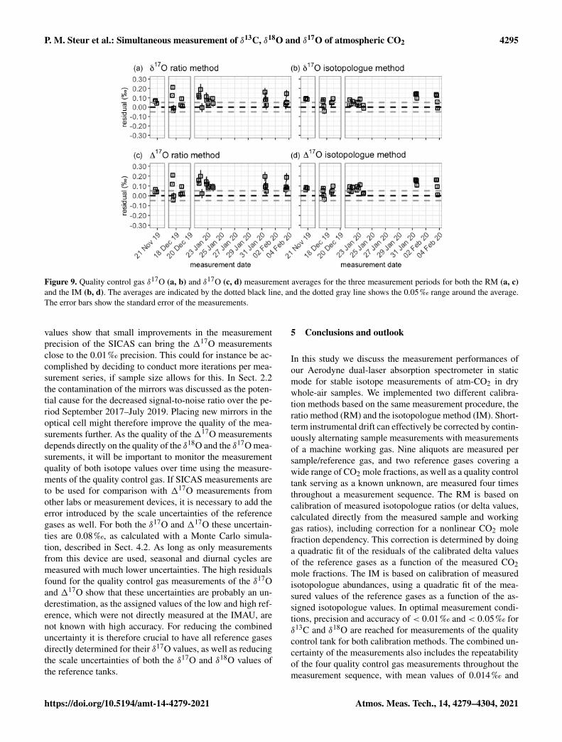
P. M. Steur et al.: Simultaneous measurement of δ13C, δ18O and δ17O of atmospheric CO2 4295
Figure 9. Quality control gas δ17O (a, b) and δ17O (c, d) measurement averages for the three measurement periods for both the RM (a, c)and the IM (b, d). The averages are indicated by the dotted black line, and the dotted gray line shows the 0.05 ‰ range around the average.The error bars show the standard error of the measurements.
values show that small improvements in the measurementprecision of the SICAS can bring the 117O measurementsclose to the 0.01 ‰ precision. This could for instance be ac-complished by deciding to conduct more iterations per mea-surement series, if sample size allows for this. In Sect. 2.2the contamination of the mirrors was discussed as the poten-tial cause for the decreased signal-to-noise ratio over the pe-riod September 2017–July 2019. Placing new mirrors in theoptical cell might therefore improve the quality of the mea-surements further. As the quality of the 117O measurementsdepends directly on the quality of the δ18O and the δ17O mea-surements, it will be important to monitor the measurementquality of both isotope values over time using the measure-ments of the quality control gas. If SICAS measurements areto be used for comparison with 117O measurements fromother labs or measurement devices, it is necessary to add theerror introduced by the scale uncertainties of the referencegases as well. For both the δ17O and 117O these uncertain-ties are 0.08 ‰, as calculated with a Monte Carlo simula-tion, described in Sect. 4.2. As long as only measurementsfrom this device are used, seasonal and diurnal cycles aremeasured with much lower uncertainties. The high residualsfound for the quality control gas measurements of the δ17Oand 117O show that these uncertainties are probably an un-derestimation, as the assigned values of the low and high ref-erence, which were not directly measured at the IMAU, arenot known with high accuracy. For reducing the combineduncertainty it is therefore crucial to have all reference gasesdirectly determined for their δ17O values, as well as reducingthe scale uncertainties of both the δ17O and δ18O values ofthe reference tanks.
5 Conclusions and outlook
In this study we discuss the measurement performances ofour Aerodyne dual-laser absorption spectrometer in staticmode for stable isotope measurements of atm-CO2 in drywhole-air samples. We implemented two different calibra-tion methods based on the same measurement procedure, theratio method (RM) and the isotopologue method (IM). Short-term instrumental drift can effectively be corrected by contin-uously alternating sample measurements with measurementsof a machine working gas. Nine aliquots are measured persample/reference gas, and two reference gases covering awide range of CO2 mole fractions, as well as a quality controltank serving as a known unknown, are measured four timesthroughout a measurement sequence. The RM is based oncalibration of measured isotopologue ratios (or delta values,calculated directly from the measured sample and workinggas ratios), including correction for a nonlinear CO2 molefraction dependency. This correction is determined by doinga quadratic fit of the residuals of the calibrated delta valuesof the reference gases as a function of the measured CO2mole fractions. The IM is based on calibration of measuredisotopologue abundances, using a quadratic fit of the mea-sured values of the reference gases as a function of the as-signed isotopologue values. In optimal measurement condi-tions, precision and accuracy of < 0.01 ‰ and < 0.05 ‰ forδ13C and δ18O are reached for measurements of the qualitycontrol tank for both calibration methods. The combined un-certainty of the measurements also includes the repeatabilityof the four quality control gas measurements throughout themeasurement sequence, with mean values of 0.014 ‰ and
https://doi.org/10.5194/amt-14-4279-2021 Atmos. Meas. Tech., 14, 4279–4304, 2021

4296 P. M. Steur et al.: Simultaneous measurement of δ13C, δ18O and δ17O of atmospheric CO2
0.012 ‰. The last components in the combined uncertaintycalculation are caused by scale uncertainties of the referencegases used for the sample calibration, which are 0.03 ‰ and0.05 ‰ for δ13C and δ18O of the RM, respectively, and0.03 ‰ and 0.06 ‰ for δ13C and δ18O of the IM, respec-tively.
A comparison of SICAS results, for both calibration meth-ods, with results from the MPI-BGC from the sausage ICPshows that sample results within the CO2 mole fraction rangeof both methods are of similar quality when compared to theMPI-BGC results. Better results were achieved for the IMfor samples outside the CO2 mole fraction range, but moremeasurements are needed to determine whether the IM is in-deed less vulnerable to extrapolation of the calibration. Asextrapolation should at any time be avoided, using referencegases that cover the range of atmospheric samples is advis-able for more reliable measurement results. We found thatδ18O measurements were consequently too depleted due tostorage times of the CIO flasks being too long before mea-surement. Future investigations will give more insight intothe stability of the oxygen isotopes within the CIO flasks,and we will evaluate the possibility of a correction based onstorage time.
δ17O and117O results of the quality control gas show val-ues that are consequently too enriched, which is probablycaused due to the indirect determination of the δ17O valuesof two of the reference gases. The measurement precision issignificantly better for the IM, with standard errors not higherthan 0.02 ‰, while the measurement precision of the RMshows standard errors ranging between 0.02 ‰ and 0.05 ‰.Results of the IM come close to the required 0.01 ‰ preci-sion to capture seasonal variations of the atmospheric 117Osignal. For a combined uncertainty of the δ17O and117O val-ues, an additional uncertainty of 0.08 ‰ must be added dueto effects of the scale uncertainties of the reference gases,indicating that improved determination of the oxygen sta-ble isotope values of the reference gases will be essential toreach high-precision 117O measurements that are compat-ible with measurements from other labs. We will show theactual achievements of 117O measurements with this instru-ment for a record of atmospheric CO2 samples of our atmo-spheric monitoring station Lutjewad in a forthcoming paper.
Atmos. Meas. Tech., 14, 4279–4304, 2021 https://doi.org/10.5194/amt-14-4279-2021
P. M. Steur et al.: Simultaneous measurement of δ13C, δ18O and δ17O of atmospheric CO2 4297
Appendix A: Preparation procedure for CO2-in-airsamples
The pure CO2 aliquots were prepared by connecting a 20 mLflask containing a pure CO2 local reference gas to a cali-brated adjustable volume. The required amount of CO2 inthe adjustable volume could be determined by measuring thepressure at a resolution of 1 mbar using a pressure sensor(Keller LEO 2). Both the sample flask and adjustable volumewere connected to a vacuum (3.3×10⁻⁵ mbar) glass line. TheCO2 in the adjustable volume was transferred cryogenically(using liquid nitrogen) into a small glass tube shape attach-ment on the side of the evacuated sample flask which wascustom-made for this purpose, and subsequently the zero-airdilutor gas was added. The dilutor gas consists of natural airscrubbed of CO2 and H2O using Ascarite® (sodium hydrox-ide coated silica, Sigma-Aldrich) and Sicapent® (phosphoricanhydride, phosphorus(V) oxide), which results in dry, CO2-free natural air. For experiment 2, additional samples wereprepared using synthetic air mixtures with and without 1 %Argon as dilutor gas for evaluation of the effect of air com-position on the CMFD (see also Sect. 3.1.6). After closingthe flask, the mixture was put to rest for at least one nightbefore measurement to ensure the CO2 and the dilutor werecompletely mixed.
Appendix B: Equations for calculation of isotopologuemole fractions
Individual isotopologues of standards of known CO2 molefractions and isotope composition are calculated for theIM calibration method by the equations below, accord-ing to Flores et al. (2017), starting with equations for theatomic abundances X in each of the calibration gas mixtures(Eqs. B1–B5):
X(
12C)=
11+R13 (B1)
X(
13C)=
R13
1+R13 (B2)
X(
16O)=
11+R18+R17 (B3)
X(
17O)=
R17
1+R18+R17 (B4)
X(
18O)=
R18
1+R18+R17 , (B5)
where
R13= R13
VPDB-CO2·
(1+ δ13C
)(B6)
R17= R17
VPDB-CO2·
(1+ δ18O
)λ(B7)
R18= R18
VPDB-CO2·
(1+ δ18O
)(B8)
and δ13C and δ18O are the delta values.R13
VPDB-CO2(0.011180), R17
VPDB-CO2(0.0003931) and
R18VPDB-CO2
(0.00208835) values were taken from Brandet al. (2010) for VPDB-CO2. Then each carbon dioxide iso-topologue mole fraction in the reference gas was calculatedaccording to its composition using Eqs. (B9) and (B10):
X626 =(X(
12C)·X(
16O)·X(
16O))·XCO2 (B9)
X636 =(X(
13C)·X(
16O)·X(
16O))·XCO2 (B10)
X628 =(X(
12C)·X(
16O)·X(
18O))· 2 ·XCO2 (B11)
X627 =(X(
12C)·X(
16O)·X(
17O))· 2 ·XCO2 . (B12)
For a more elaborated explanation of these equations, seeFlores et al. (2017).
Appendix C: Step-by-step calculation steps
C1 Ratio method
1. Calculate ratios from the measured isotopologue abun-dances:
r∗ =X∗
X626, (C1)
with r being the ratio, X the measured isotopologueabundance as the default output, scaled in this way forthe natural abundance, ∗ stands for one of the three rareisotopologues (636, 628 or 627) and 626 standard forthe abundant isotopologue. The CO2 mole fraction iscalculated by
[CO2]= A626+A636+A628+A627, (C2)
withA being the actual measured abundance, calculatedback in this way using the natural abundance values forthe isotopologues as defined in Rothman et al. (2013).
2. Use only the relevant interval (in our case 30–60 s) frommeasured ratio and [CO2] per measurement.
3. Do a drift correction and calculate the uncalibrated deltavalue by
δ∗S(t)dc=rS(t)
rWG(t)− 1, (C3)
with S for sample, t for time of the measurement,dc for drift-corrected and WG for working gas and withr∗WG(t) derived from applying a time-dependent linear fitof the r∗WG(t−1) and r∗WG(t+1), following
r∗WG(t) = α+β · t. (C4)
The [CO2] is also drift-corrected by
https://doi.org/10.5194/amt-14-4279-2021 Atmos. Meas. Tech., 14, 4279–4304, 2021
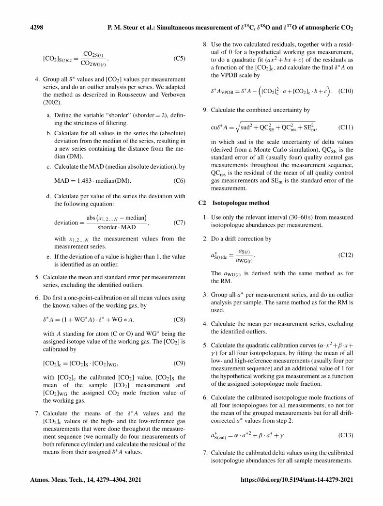
4298 P. M. Steur et al.: Simultaneous measurement of δ13C, δ18O and δ17O of atmospheric CO2
[CO2]S(t)dc =CO2S(t)
CO2WG(t). (C5)
4. Group all δ∗ values and [CO2] values per measurementseries, and do an outlier analysis per series. We adaptedthe method as described in Rousseeuw and Verboven(2002).
a. Define the variable “sborder” (sborder= 2), defin-ing the strictness of filtering.
b. Calculate for all values in the series the (absolute)deviation from the median of the series, resulting ina new series containing the distance from the me-dian (DM).
c. Calculate the MAD (median absolute deviation), by
MAD= 1.483 ·median(DM). (C6)
d. Calculate per value of the series the deviation withthe following equation:
deviation=abs
(x1,2 ... N −median
)sborder ·MAD
, (C7)
with x1,2 ... N the measurement values from themeasurement series.
e. If the deviation of a value is higher than 1, the valueis identified as an outlier.
5. Calculate the mean and standard error per measurementseries, excluding the identified outliers.
6. Do first a one-point-calibration on all mean values usingthe known values of the working gas, by
δ∗A= (1+WG∗A) · δ∗+WG ∗A, (C8)
with A standing for atom (C or O) and WG∗ being theassigned isotope value of the working gas. The [CO2] iscalibrated by
[CO2]c = [CO2]S · [CO2]WG, (C9)
with [CO2]c the calibrated [CO2] value, [CO2]S themean of the sample [CO2] measurement and[CO2]WG the assigned CO2 mole fraction value ofthe working gas.
7. Calculate the means of the δ∗A values and the[CO2]c values of the high- and the low-reference gasmeasurements that were done throughout the measure-ment sequence (we normally do four measurements ofboth reference cylinder) and calculate the residual of themeans from their assigned δ∗A values.
8. Use the two calculated residuals, together with a resid-ual of 0 for a hypothetical working gas measurement,to do a quadratic fit (ax2
+ bx+ c) of the residuals asa function of the [CO2]c, and calculate the final δ∗A onthe VPDB scale by
δ∗AVPDB = δ∗A−
([CO2]2
c · a+ [CO2]c · b+ c). (C10)
9. Calculate the combined uncertainty by
cuδ∗A=√
sud2+QC2
SE+QC2res+SE2
m, (C11)
in which sud is the scale uncertainty of delta values(derived from a Monte Carlo simulation), QCSE is thestandard error of all (usually four) quality control gasmeasurements throughout the measurement sequence,QCres is the residual of the mean of all quality controlgas measurements and SEm is the standard error of themeasurement.
C2 Isotopologue method
1. Use only the relevant interval (30–60 s) from measuredisotopologue abundances per measurement.
2. Do a drift correction by
a∗S(t)dc =aS(t)
aWG(t). (C12)
The aWG(t) is derived with the same method as forthe RM.
3. Group all a∗ per measurement series, and do an outlieranalysis per sample. The same method as for the RM isused.
4. Calculate the mean per measurement series, excludingthe identified outliers.
5. Calculate the quadratic calibration curves (α ·x2+β ·x+
γ ) for all four isotopologues, by fitting the mean of alllow- and high-reference measurements (usually four permeasurement sequence) and an additional value of 1 forthe hypothetical working gas measurement as a functionof the assigned isotopologue mole fraction.
6. Calculate the calibrated isotopologue mole fractions ofall four isotopologues for all measurements, so not forthe mean of the grouped measurements but for all drift-corrected a∗ values from step 2:
a∗S(cal) = α · a∗2+β · a∗+ γ. (C13)
7. Calculate the calibrated delta values using the calibratedisotopologue abundances for all sample measurements.
Atmos. Meas. Tech., 14, 4279–4304, 2021 https://doi.org/10.5194/amt-14-4279-2021
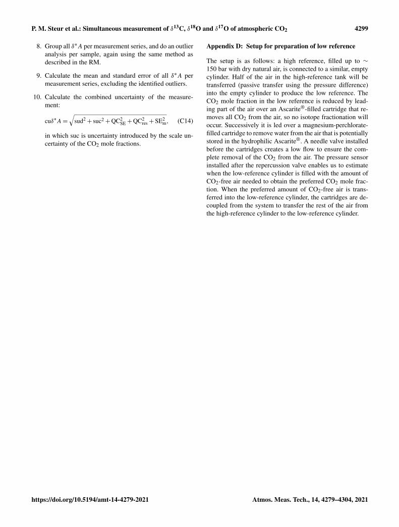
P. M. Steur et al.: Simultaneous measurement of δ13C, δ18O and δ17O of atmospheric CO2 4299
8. Group all δ∗A per measurement series, and do an outlieranalysis per sample, again using the same method asdescribed in the RM.
9. Calculate the mean and standard error of all δ∗A permeasurement series, excluding the identified outliers.
10. Calculate the combined uncertainty of the measure-ment:
cuδ∗A=√
sud2+ suc2+QC2
SE+QC2res+SE2
m, (C14)
in which suc is uncertainty introduced by the scale un-certainty of the CO2 mole fractions.
Appendix D: Setup for preparation of low reference
The setup is as follows: a high reference, filled up to ∼150 bar with dry natural air, is connected to a similar, emptycylinder. Half of the air in the high-reference tank will betransferred (passive transfer using the pressure difference)into the empty cylinder to produce the low reference. TheCO2 mole fraction in the low reference is reduced by lead-ing part of the air over an Ascarite®-filled cartridge that re-moves all CO2 from the air, so no isotope fractionation willoccur. Successively it is led over a magnesium-perchlorate-filled cartridge to remove water from the air that is potentiallystored in the hydrophilic Ascarite®. A needle valve installedbefore the cartridges creates a low flow to ensure the com-plete removal of the CO2 from the air. The pressure sensorinstalled after the repercussion valve enables us to estimatewhen the low-reference cylinder is filled with the amount ofCO2-free air needed to obtain the preferred CO2 mole frac-tion. When the preferred amount of CO2-free air is trans-ferred into the low-reference cylinder, the cartridges are de-coupled from the system to transfer the rest of the air fromthe high-reference cylinder to the low-reference cylinder.
https://doi.org/10.5194/amt-14-4279-2021 Atmos. Meas. Tech., 14, 4279–4304, 2021

4300 P. M. Steur et al.: Simultaneous measurement of δ13C, δ18O and δ17O of atmospheric CO2
Figure D1. Setup for the preparation of the low reference. The cylinder on the left is the high reference, filled until ∼ 150 bar at start time ofpreparation. The right cylinder is empty at start time of preparation.
Atmos. Meas. Tech., 14, 4279–4304, 2021 https://doi.org/10.5194/amt-14-4279-2021

P. M. Steur et al.: Simultaneous measurement of δ13C, δ18O and δ17O of atmospheric CO2 4301
Appendix E: Analysis cross-contamination
To determine whether cross-contamination has the potentialto affect isotope measurements on the SICAS, a simulationwas conducted in which we use the measurement proceduredescribed in this paper. Input in the simulation is an exper-imentally derived value, which expresses how much a mea-sured sample is affected by the sample that was measured inthe optical cell before. The experiment was conducted as fol-lows: the high reference was measured eight times in a row,each time letting in a new aliquot, followed by the low refer-ence which was also measured eight times in a row, and thisprocedure was repeated three times. The usual flushing pro-cedure was applied every time there was a switch between thecylinders. It can be expected that the first measurement of aseries of eight of the low reference is affected the most by thepreceding measurement of the high-reference gas. The lastmeasurements of a series of eight will be affected less andwill be closer to the “true” value. We quantified this effectby applying the following equation to all series of measuredisotopologues:
CC=M∗1 −mean
(M∗6,7,8
)mean
(M∗6,7,8
) · 100, (E1)
in which CC is the cross-contamination in percent, andM stands for measurement, with ∗ being the isotopologueand the number indicated at the underscore the number of themeasurement. The CC values we observed were low, rangingfrom undetectable up to 0.01 % at most. We used this highestvalue for our simulation.
A simulation for a measurement sequence was set up inExcel, following the measurement procedure as described inthis paper, only using three sample measurements per mea-surement series instead of nine. Included in the simulationare measurements of the low- and high-reference gas and twohypothetical samples with CO2 concentrations of 480 and340 ppm, a δ13C values of −7 ‰ and −11 ‰ and δ18O val-ues of −1 ‰ and −4 ‰, respectively. All measurements arealternated with measurements of the working gas, accordingto the measurement procedure described in this paper. We usethe actual values for CO2 concentration and isotope compo-sition of all reference gases in the simulation. The measure-ments were simulated by
M∗t =M∗
t−1 · 0.01× 10−2+
(1− 0.01× 10⁻²
)·Tr∗, (E2)
with M∗t being the simulated measurement at time t and∗ indicating which isotopologue measurement is simulated,Mt−1 being the preceding simulated measurement and Tr be-ing the true isotopologue abundance of the sample or ref-erence gas that is being measured at time t . The first valuethat is put in the simulation contains the true values for allmeasured isotopologue abundances. For all sample measure-ments, a normalized measurement is calculated by divid-ing M∗t by M∗t−1 (being the working gas measurement).
These simulated, normalized measurements of the low-and high-reference gases are used to do a linear fit as a func-tion of the true value and in doing so calculate the calibrationcurves. These curves are used to calculate the calibrated sam-ple measurements, and the measured δ13C and δ18O mea-surements can be calculated. We find deviations from themeasured simulation values of maximum 0.0002 ‰ for bothδ13C and δ18O, so 2 orders of magnitude lower than the mea-surement precision.
https://doi.org/10.5194/amt-14-4279-2021 Atmos. Meas. Tech., 14, 4279–4304, 2021
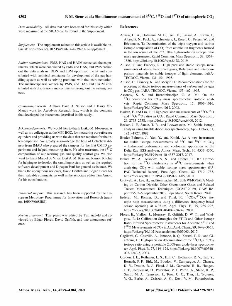
4302 P. M. Steur et al.: Simultaneous measurement of δ13C, δ18O and δ17O of atmospheric CO2
Data availability. All data that have been used for this study whichwere measured at the SICAS can be found in the Supplement.
Supplement. The supplement related to this article is available on-line at: https://doi.org/10.5194/amt-14-4279-2021-supplement.
Author contributions. PMS, HAS and HAJM conceived the exper-iments, which were conducted by PMS and HAS, and PMS carriedout the data analysis. DDN and JBM optimized the fit and con-tributed with technical assistance for development of the gas han-dling system as well as solving problems with the instrumentation.The manuscript was written by PMS, and HAS and HAJM con-tributed with discussions and comments throughout the writing pro-cess.
Competing interests. Authors Dave D. Nelson and J. Barry Mc-Manus work for Aerodyne Research Inc., which is the companythat developed the instrument described in this study.
Acknowledgements. We would like to thank Heiko M. Moossen, aswell as his colleagues at the MPI-BGC, for measuring our referencecylinders and providing us with the data that we required for the in-tercomparison. We greatly acknowledge the help of Getachew Ad-new from IMAU who prepared the samples for the first CMFD ex-periment and helped measuring them. He also measured the δ17Ocomposition of our working gas and quality control gas. We alsowant to thank Marcel de Vries, Bert A. M. Kers and Ramon Ritchiefor helping us to develop the sampling system as well as the requiredsoftware development and Dipayan Paul for general assistance. Wethank the anonymous reviewer, David Griffith and Edgar Flores fortheir valuable comments, as well as the associate editor Tim Arnoldfor his contributions.
Financial support. This research has been supported by the Eu-ropean Metrology Programme for Innovation and Research (grantno. 16ENV06SIRS).
Review statement. This paper was edited by Tim Arnold and re-viewed by Edgar Flores, David Griffith, and one anonymous ref-eree.
References
Adnew, G. A., Hofmann, M. E., Paul, D., Laskar, A., Surma, J.,Albrecht, N., Pack, A., Schwieters, J., Koren, G., Peters, W., andRöckmann, T.: Determination of the triple oxygen and carbonisotopic composition of CO2 from atomic ion fragments formedin the ion source of the 253 Ultra high-resolution isotope ratiomass spectrometer, Rapid Commun. Mass Spectrom., 33, 1363–1380, https://doi.org/10.1002/rcm.8478, 2019.
Allison, C. and Francey, R.: High precision stable isotope mea-surements of atmospheric trace gases, Reference and intercom-parison materials for stable isotopes of light elements, IAEA-TECDOC, Vienna, 131–154, 1995.
Allison, C., Francey, R., and Meijer, H.: Recommendations for thereporting of stable isotope measurements of carbon and oxygenin CO2 gas, IAEA-TECDOC, Vienna, 155–162, 1995.
Assonov, S. S. and Brenninkmeijer, C. A. M.: On the17O correction for CO2 mass spectrometric isotopic anal-ysis, Rapid Commun. Mass Spectrom., 17, 1007–1016,https://doi.org/10.1002/rcm.1012, 2003.
Barkan, E. and Luz, B.: High-precision measurements of 17O/16Oand 18O/16O ratios in CO2, Rapid Commun. Mass Spectrom.,26, 2733–2738, https://doi.org/10.1002/rcm.6400, 2012.
Becker, J. F., Sauke, T. B., and Loewenstein, M.: Stable isotopeanalysis using tunable diode laser spectroscopy, Appl. Optics, 31,1921–1927, 1992.
Braden-Behrens, J., Yan, Y., and Knohl, A.: A new instrumentfor stable isotope measurements of 13C and 18O in CO2– Instrument performance and ecological application of theDelta Ray IRIS analyzer, Atmos. Meas. Tech., 10, 4537–4560,https://doi.org/10.5194/amt-10-4537-2017, 2017.
Brand, W. A., Assonov, S. S., and Coplen, T. B.: Correc-tion for the 17O interference in δ13C measurements whenanalyzing CO2 with stable isotope mass spectrometry (IU-PAC Technical Report), Pure Appl. Chem., 82, 1719–1733,https://doi.org/10.1351/PAC-REP-09-01-05, 2010.
Crotwell, A., Lee, H., and Steinbacher, M.: 20th WMO/IAEA Meet-ing on Carbon Dioxide, Other Greenhouse Gases and RelatedTracers Measurement Techniques (GGMT-2019), GAW Re-port 255, 2–5 September 2019, Jeju Island, South Korea, 2020.
Erdélyi, M., Richter, D., and Tittel, F.: 13CO2/12CO2 iso-
topic ratio measurements using a difference frequency-basedsensor operating at 4.35 µm, Appl. Phys. B, 75, 289–295,https://doi.org/10.1007/s00340-002-0960-2, 2002.
Flores, E., Viallon, J., Moussay, P., Griffith, D. W. T., and Wiel-gosz, R. I.: Calibration Strategies for FT-IR and Other IsotopeRatio Infrared Spectrometer Instruments for Accurate δ13C andδ18O Measurements of CO2 in Air, Anal. Chem., 89, 3648–3655,https://doi.org/10.1021/acs.analchem.6b05063, 2017.
Gagliardi, G., Castrillo, A., Iannone, R. Q., Kerstel, E. R., and Gi-anfrani, L.: High-precision determination of the 13CO2/
12CO2isotope ratio using a portable 2.008-µm diode-laser spectrome-ter, Appl. Phys. B, 77, 119–124, https://doi.org/10.1007/s00340-003-1240-5, 2003.
Gordon, I. E., Rothman, L. S., Hill, C., Kochanov, R. V., Tan, Y.,Bernath, P. F., Birk, M., Boudon, V., Campargue, A., Chance,K. V., Drouin, B. J., Flaud, J. M., Gamache, R. R., Hodges,J. T., Jacquemart, D., Perevalov, V. I., Perrin, A., Shine, K. P.,Smith, M. A., Tennyson, J., Toon, G. C., Tran, H., Tyuterev,V. G., Barbe, A., Császár, A. G., Devi, V. M., Furtenbacher,
Atmos. Meas. Tech., 14, 4279–4304, 2021 https://doi.org/10.5194/amt-14-4279-2021

P. M. Steur et al.: Simultaneous measurement of δ13C, δ18O and δ17O of atmospheric CO2 4303
T., Harrison, J. J., Hartmann, J. M., Jolly, A., Johnson, T. J.,Karman, T., Kleiner, I., Kyuberis, A. A., Loos, J., Lyulin, O.M., Massie, S. T., Mikhailenko, S. N., Moazzen-Ahmadi, N.,Müller, H. S., Naumenko, O. V., Nikitin, A. V., Polyansky, O.L., Rey, M., Rotger, M., Sharpe, S. W., Sung, K., Starikova,E., Tashkun, S. A., Auwera, J. V., Wagner, G., Wilzewski, J.,Wcisło, P., Yu, S., and Zak, E. J.: The HITRAN2016 molecu-lar spectroscopic database, J. Quant. Spectrosc. Ra., 203, 3–69,https://doi.org/10.1016/j.jqsrt.2017.06.038, 2017.
Griffith, D. W.: Calibration of isotopologue-specific optical tracegas analysers: A practical guide, Atmos. Meas. Tech., 11, 6189–6201, https://doi.org/10.5194/amt-11-6189-2018, 2018.
Griffith, D. W., Deutscher, N. M., Caldow, C., Kettlewell, G.,Riggenbach, M., and Hammer, S.: A Fourier transform infraredtrace gas and isotope analyser for atmospheric applications, At-mos. Meas. Tech., 5, 2481–2498, https://doi.org/10.5194/amt-5-2481-2012, 2012.
Harris, S. J., Liisberg, J., Xia, L., Wei, J., Zeyer, K., Yu, L., Barthel,M., Wolf, B., Kelly, B. F., Cendón, D. I., Blunier, T., Six, J.,and Mohn, J.: N2O isotopocule measurements using laser spec-troscopy: Analyzer characterization and intercomparison, At-mos. Meas. Tech., 13, 2797–2831, https://doi.org/10.5194/amt-13-2797-2020, 2020.
Hoag, K. J., Still, C. J., Fung, I. Y., and Boering, K. A.: Tripleoxygen isotope composition of tropospheric carbon dioxide asa tracer of terrestrial gross carbon fluxes, Geophys. Res. Lett.,32, 1–5, https://doi.org/10.1029/2004GL021011, 2005.
Hofmann, M. and Pack, A.: Development of a technique for high-precision analysis of triple oxygen isotope ratios in carbon diox-ide, Anal. Chem., 82, 4357–4361, 2010.
Hofmann, M. E. G., Horváth, B., Schneider, L., Peters, W.,Schützenmeister, K., and Pack, A.: Atmospheric measurementsof 117O in CO2 in Göttingen, Germany reveal a seasonal cycledriven by biospheric uptake, Geochim. Cosmochim. Ac., 199,143–163, https://doi.org/10.1016/j.gca.2016.11.019, 2017.
Horváth, B., Hofmann, M. E., and Pack, A.: On the triple oxy-gen isotope composition of carbon dioxide from some com-bustion processes, Geochim. Cosmochim. Ac., 95, 160–168,https://doi.org/10.1016/j.gca.2012.07.021, 2012.
IAEA: Stable isotope measurement techniques for atmosphericgreenhouse gases, IAEA-TECDOC, Vienna, 2002.
IAEA: Reference Sheet: Certified Reference Material: IAEA-603(calcite) – Stable Isotope Reference Material, available at: https://nucleus.iaea.org/rpst/ReferenceProducts/ReferenceMaterials/Stable_Isotopes/13C18and7Li/IAEA-603.htm (last access:28 May 2021), 2016.
Kerstel, E. R., Van Trigt, R., Dam, N., Reuss, J., and Mei-jer, H. A. J.: Simultaneous determination of the 2H/1H,17O/16O, and 18O/16O isotope abundance ratios in water bymeans of laser spectrometry, Anal. Chem., 71, 5297–5303,https://doi.org/10.1021/ac990621e, 1999.
Koren, G., Schneider, L., van der Velde, I. R., van Schaik, E., Gro-mov, S. S., Adnew, G. A., Mrozek Martino, D. J., Hofmann, M.E. G., Liang, M.-C., Mahata, S., Bergamaschi, P., van der Laan-Luijkx, I. T., Krol, M. C., Röckmann, T., and Peters, W.: Global3-D Simulations of the Triple Oxygen Isotope Signature 117Oin Atmospheric CO2, J. Geophys. Res.-Atmos., 124, 8808–8836,https://doi.org/10.1029/2019jd030387, 2019.
Laskar, A. H., Mahata, S., and Liang, M. C.: Identifi-cation of Anthropogenic CO2 Using Triple Oxygen andClumped Isotopes, Environ. Sci. Technol., 50, 11806–11814,https://doi.org/10.1021/acs.est.6b02989, 2016.
Leuenberger, M. C., Schibig, M. F., and Nyfeler, P.: Gas adsorp-tion and desorption effects on cylinders and their importancefor long-term gas records, Atmos. Meas. Tech., 8, 5289–5299,https://doi.org/10.5194/amt-8-5289-2015, 2015.
Levin, I., Facklam, C., Schmidt, M., Ramonet, M., Ciais, P., Xueref,I., Langenfelds, R., Allison, C., Francey, R., Jordan, A., Rothe,M., Brand, W. A., Neubert, R. E., Meijer, H. A. J., Machida, T.,and Mukai, H.: Results of inter-comparison programme for anal-ysis of “sausage” flask air samples, Special report 2, Terrestrialand Atmospheric Carbon Observing System Infrastructure, Gif-Sur-Yvette, France, 2004.
Liang, M. C., Mahata, S., Laskar, A. H., and Bhattacharya, S.K.: Spatiotemporal variability of oxygen isotope anomaly innear surface air CO2 over urban, semi-urban and ocean areasin and around Taiwan, Aerosol Air Qual. Res., 17, 706–720,https://doi.org/10.4209/aaqr.2016.04.0171, 2017.
Luz, B., Barkan, E., and Bender, M. L.: Triple-isotope compositionof atmospheric oxygen as a tracer of biosphere productivity, Lett.Nat., 400, 547–550, 1999.
Mahata, S., Bhattacharya, S. K., Wang, C. H., and Liang,M. C.: Oxygen isotope exchange between O2 and CO2over hot platinum: An innovative technique for mea-suring 117O in CO2, Anal. Chem., 85, 6894–6901,https://doi.org/10.1021/ac4011777, 2013.
McManus, J. B., Nelson, D. D., Shorter, J. H., Jimenez, R.,Herndon, S., Saleska, S., and Zahniser, M.: A high preci-sion pulsed quantum cascade laser for measurements of sta-ble isotopes of carbon dioxide, J. Modern Opt., 52, 2309–2321,https://doi.org/10.1080/09500340500303710, 2005.
McManus, J. B., Nelson, D. D., and Zahniser, M. S.: Designand performance of a dual-laser instrument for multiple iso-topologues of carbon dioxide and water, Opt. Exp., 23, 6569,https://doi.org/10.1364/OE.23.006569, 2015.
Meijer, H. A. J.: Stable isotope quality assurance using the ‘Cali-brated IRMS’ strategy, Isotop. Environ. Health Stud., 45, 150–163, https://doi.org/10.1080/10256010902869113, 2009.
Meijer, H. A. J., Neubert, R. E. M., and Visser, G. H.: Cross con-tamination in dual inlet isotope ratio mass spectrometers, Int.J. Mass Spectrom., 198, 45–61, https://doi.org/10.1016/S1387-3806(99)00266-3, 2000.
Mrozek, D. J., Van Der Veen, C., Hofmann, M. E., Chen, H., Kivi,R., Heikkinen, P., and Röckmann, T.: Stratospheric Air Sub-sampler (SAS) and its application to analysis of 117O(CO2)from small air samples collected with an AirCore, Atmos. Meas.Tech., 9, 5607–5620, https://doi.org/10.5194/amt-9-5607-2016,2016.
Murnick, D. E. and Peer, B. J.: Laser-based analysis of carbon iso-tope ratios, Science, 263, 945–947, 1994.
Nakamichi, S., Kawaguchi, Y., Fukuda, H., Enami, S., Hashimoto,S., Kawasaki, M., Umekawa, T., Morino, I., Suto, H.,and Inoue, G.: Buffer-gas pressure broadening for the(3001)III (0 0 0) band of CO2 measured with continuous-wave cavity ring-down spectroscopy, Chem. Phys., 8, 364–368,https://doi.org/10.1039/B511772K, 2006.
https://doi.org/10.5194/amt-14-4279-2021 Atmos. Meas. Tech., 14, 4279–4304, 2021
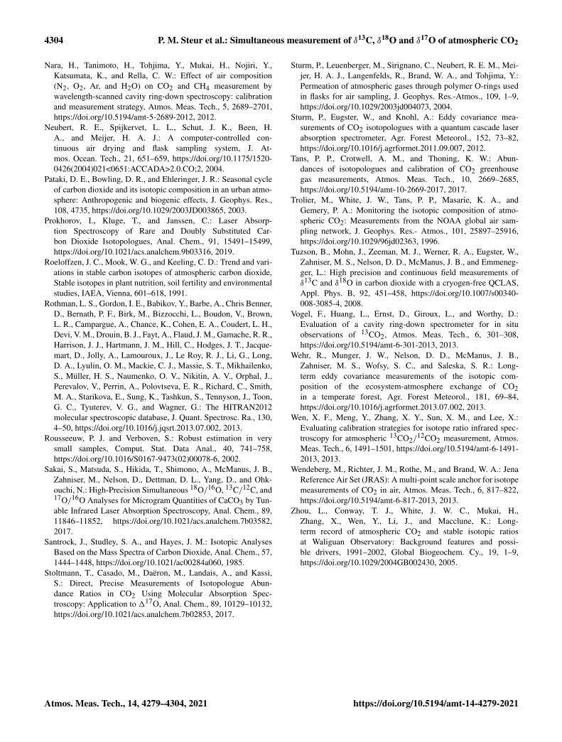
4304 P. M. Steur et al.: Simultaneous measurement of δ13C, δ18O and δ17O of atmospheric CO2
Nara, H., Tanimoto, H., Tohjima, Y., Mukai, H., Nojiri, Y.,Katsumata, K., and Rella, C. W.: Effect of air composition(N2, O2, Ar, and H2O) on CO2 and CH4 measurement bywavelength-scanned cavity ring-down spectroscopy: calibrationand measurement strategy, Atmos. Meas. Tech., 5, 2689–2701,https://doi.org/10.5194/amt-5-2689-2012, 2012.
Neubert, R. E., Spijkervet, L. L., Schut, J. K., Been, H.A., and Meijer, H. A. J.: A computer-controlled con-tinuous air drying and flask sampling system, J. At-mos. Ocean. Tech., 21, 651–659, https://doi.org/10.1175/1520-0426(2004)021<0651:ACCADA>2.0.CO;2, 2004.
Pataki, D. E., Bowling, D. R., and Ehleringer, J. R.: Seasonal cycleof carbon dioxide and its isotopic composition in an urban atmo-sphere: Anthropogenic and biogenic effects, J. Geophys. Res.,108, 4735, https://doi.org/10.1029/2003JD003865, 2003.
Prokhorov, I., Kluge, T., and Janssen, C.: Laser Absorp-tion Spectroscopy of Rare and Doubly Substituted Car-bon Dioxide Isotopologues, Anal. Chem., 91, 15491–15499,https://doi.org/10.1021/acs.analchem.9b03316, 2019.
Roeloffzen, J. C., Mook, W. G., and Keeling, C. D.: Trend and vari-ations in stable carbon isotopes of atmospheric carbon dioxide,Stable isotopes in plant nutrition, soil fertility and environmentalstudies, IAEA, Vienna, 601–618, 1991.
Rothman, L. S., Gordon, I. E., Babikov, Y., Barbe, A., Chris Benner,D., Bernath, P. F., Birk, M., Bizzocchi, L., Boudon, V., Brown,L. R., Campargue, A., Chance, K., Cohen, E. A., Coudert, L. H.,Devi, V. M., Drouin, B. J., Fayt, A., Flaud, J. M., Gamache, R. R.,Harrison, J. J., Hartmann, J. M., Hill, C., Hodges, J. T., Jacque-mart, D., Jolly, A., Lamouroux, J., Le Roy, R. J., Li, G., Long,D. A., Lyulin, O. M., Mackie, C. J., Massie, S. T., Mikhailenko,S., Müller, H. S., Naumenko, O. V., Nikitin, A. V., Orphal, J.,Perevalov, V., Perrin, A., Polovtseva, E. R., Richard, C., Smith,M. A., Starikova, E., Sung, K., Tashkun, S., Tennyson, J., Toon,G. C., Tyuterev, V. G., and Wagner, G.: The HITRAN2012molecular spectroscopic database, J. Quant. Spectrosc. Ra., 130,4–50, https://doi.org/10.1016/j.jqsrt.2013.07.002, 2013.
Rousseeuw, P. J. and Verboven, S.: Robust estimation in verysmall samples, Comput. Stat. Data Anal., 40, 741–758,https://doi.org/10.1016/S0167-9473(02)00078-6, 2002.
Sakai, S., Matsuda, S., Hikida, T., Shimono, A., McManus, J. B.,Zahniser, M., Nelson, D., Dettman, D. L., Yang, D., and Ohk-ouchi, N.: High-Precision Simultaneous 18O/16O, 13C/12C, and17O/16O Analyses for Microgram Quantities of CaCO3 by Tun-able Infrared Laser Absorption Spectroscopy, Anal. Chem., 89,11846–11852, https://doi.org/10.1021/acs.analchem.7b03582,2017.
Santrock, J., Studley, S. A., and Hayes, J. M.: Isotopic AnalysesBased on the Mass Spectra of Carbon Dioxide, Anal. Chem., 57,1444–1448, https://doi.org/10.1021/ac00284a060, 1985.
Stoltmann, T., Casado, M., Daëron, M., Landais, A., and Kassi,S.: Direct, Precise Measurements of Isotopologue Abun-dance Ratios in CO2 Using Molecular Absorption Spec-troscopy: Application to 117O, Anal. Chem., 89, 10129–10132,https://doi.org/10.1021/acs.analchem.7b02853, 2017.
Sturm, P., Leuenberger, M., Sirignano, C., Neubert, R. E. M., Mei-jer, H. A. J., Langenfelds, R., Brand, W. A., and Tohjima, Y.:Permeation of atmospheric gases through polymer O-rings usedin flasks for air sampling, J. Geophys. Res.-Atmos., 109, 1–9,https://doi.org/10.1029/2003jd004073, 2004.
Sturm, P., Eugster, W., and Knohl, A.: Eddy covariance mea-surements of CO2 isotopologues with a quantum cascade laserabsorption spectrometer, Agr. Forest Meteorol., 152, 73–82,https://doi.org/10.1016/j.agrformet.2011.09.007, 2012.
Tans, P. P., Crotwell, A. M., and Thoning, K. W.: Abun-dances of isotopologues and calibration of CO2 greenhousegas measurements, Atmos. Meas. Tech., 10, 2669–2685,https://doi.org/10.5194/amt-10-2669-2017, 2017.
Trolier, M., White, J. W., Tans, P. P., Masarie, K. A., andGemery, P. A.: Monitoring the isotopic composition of atmo-spheric CO2: Measurements from the NOAA global air sam-pling network, J. Geophys. Res.- Atmos., 101, 25897–25916,https://doi.org/10.1029/96jd02363, 1996.
Tuzson, B., Mohn, J., Zeeman, M. J., Werner, R. A., Eugster, W.,Zahniser, M. S., Nelson, D. D., McManus, J. B., and Emmeneg-ger, L.: High precision and continuous field measurements ofδ13C and δ18O in carbon dioxide with a cryogen-free QCLAS,Appl. Phys. B, 92, 451–458, https://doi.org/10.1007/s00340-008-3085-4, 2008.
Vogel, F., Huang, L., Ernst, D., Giroux, L., and Worthy, D.:Evaluation of a cavity ring-down spectrometer for in situobservations of 13CO2, Atmos. Meas. Tech., 6, 301–308,https://doi.org/10.5194/amt-6-301-2013, 2013.
Wehr, R., Munger, J. W., Nelson, D. D., McManus, J. B.,Zahniser, M. S., Wofsy, S. C., and Saleska, S. R.: Long-term eddy covariance measurements of the isotopic com-position of the ecosystem-atmosphere exchange of CO2in a temperate forest, Agr. Forest Meteorol., 181, 69–84,https://doi.org/10.1016/j.agrformet.2013.07.002, 2013.
Wen, X. F., Meng, Y., Zhang, X. Y., Sun, X. M., and Lee, X.:Evaluating calibration strategies for isotope ratio infrared spec-troscopy for atmospheric 13CO2/
12CO2 measurement, Atmos.Meas. Tech., 6, 1491–1501, https://doi.org/10.5194/amt-6-1491-2013, 2013.
Wendeberg, M., Richter, J. M., Rothe, M., and Brand, W. A.: JenaReference Air Set (JRAS): A multi-point scale anchor for isotopemeasurements of CO2 in air, Atmos. Meas. Tech., 6, 817–822,https://doi.org/10.5194/amt-6-817-2013, 2013.
Zhou, L., Conway, T. J., White, J. W. C., Mukai, H.,Zhang, X., Wen, Y., Li, J., and Macclune, K.: Long-term record of atmospheric CO2 and stable isotopic ratiosat Waliguan Observatory: Background features and possi-ble drivers, 1991–2002, Global Biogeochem. Cy., 19, 1–9,https://doi.org/10.1029/2004GB002430, 2005.
Atmos. Meas. Tech., 14, 4279–4304, 2021 https://doi.org/10.5194/amt-14-4279-2021