Calibration of the carbon isotope composition(δ13C) of benthic foraminiferaAndreas Schmittner1 , Helen C. Bostock2 , Olivier Cartapanis3,4 , William B. Curry5,6,Helena L. Filipsson7 , Eric D. Galbraith4,8,9 , Julia Gottschalk3 , Juan Carlos Herguera10 ,Babette Hoogakker11 , Samuel L. Jaccard3 , Lorraine E. Lisiecki12 , David C. Lund13 ,Gema Martínez-Méndez14 , Jean Lynch-Stieglitz15 , Andreas Mackensen16 ,Elisabeth Michel17 , Alan C. Mix1, Delia W. Oppo6 , Carlye D. Peterson18 , Janne Repschläger19,Elisabeth L. Sikes20 , Howard J. Spero18, and Claire Waelbroeck17

1College of Earth, Ocean, and Atmospheric Sciences, Oregon State University, Corvallis, Oregon, USA, 2National Institute ofWater and Atmospheric Research, Wellington, New Zealand, 3Institute of Geological Sciences and Oeschger Center forClimate Change Research, University of Bern, Bern, Switzerland, 4Department of Earth and Planetary Sciences, McGillUniversity, Montreal, Québec, Canada, 5Bermuda Institute of Ocean Sciences, Bermuda, 6Department of Geology andGeophysics, Woods Hole Oceanographic Institution, Woods Hole, Massachusetts, USA, 7Department of Geology, LundUniversity, Lund, Sweden, 8Institut de Ciència i Tecnologia Ambientals, Universitat Autònoma de Barcelona, Barcelona,Spain, 9ICREA, Barcelona, Spain, 10Oceanología, Centro de Investigación Científica y de Educación Superior de Ensenada,Ensenada, Baja California, Mexico, 11The Lyell Centre, Heriot Watt University, Edinburgh, UK, 12Department ofEarth Sciences, University of California, Santa Barbara, California, USA, 13Department of Marine Sciences, University ofConnecticut-Avery Point, Groton, Connecticut, USA, 14MARUM-Center for Marine Environmental Sciences, Universityof Bremen, Bremen, Germany, 15School of Earth and Atmospheric Sciences, Georgia Institute of Technology, Atlanta,Georgia, USA, 16Alfred-Wegener Institute for Polar and Marine Sciences, Bremerhaven, Germany, 17LSCE/IPSL, LaboratoireCNRS-CEA-UVSQ, Gif-sur-Yvette, France, 18Department of Earth and Planetary Sciences, University of California, Davis,California, USA, 19Max Planck Institute for Chemistry, Mainz, Germany, 20Institute of Marine and Coastal Sciences, RutgersUniversity, New Brunswick, New Jersey, USA

Abstract The carbon isotope composition (δ13C) of seawater provides valuable insight on oceancirculation, air-sea exchange, the biological pump, and the global carbon cycle and is reflected by the δ13Cof foraminifera tests. Here more than 1700 δ13C observations of the benthic foraminifera genus Cibicidesfrom late Holocene sediments (δ13CCibnat) are compiled and compared with newly updated estimates ofthe natural (preindustrial) water column δ13C of dissolved inorganic carbon (δ13CDICnat) as part of theinternational Ocean Circulation and Carbon Cycling (OC3) project. Using selection criteria based on thespatial distance between samples, we find high correlation between δ13CCibnat and δ13CDICnat, confirmingearlier work. Regression analyses indicate significant carbonate ion (�2.6 ± 0.4) × 10�3‰/(μmol kg�1)[CO3

2�] and pressure (�4.9 ± 1.7) × 10�5‰ m�1 (depth) effects, which we use to propose a new globalcalibration for predicting δ13CDICnat from δ13CCibnat. This calibration is shown to remove some systematicregional biases and decrease errors compared with the one-to-one relationship (δ13CDICnat = δ13CCibnat).However, these effects and the error reductions are relatively small, which suggests that most conclusionsfrom previous studies using a one-to-one relationship remain robust. The remaining standard error of theregression is generally σ ≅ 0.25‰, with larger values found in the southeast Atlantic and Antarctic (σ ≅ 0.4‰)and for species other than Cibicides wuellerstorfi. Discussion of species effects and possible sources of theremaining errors may aid future attempts to improve the use of the benthic δ13C record.

1. Introduction

The stable carbon isotope composition (δ13C) measured in calcium carbonate shells (tests) of benthic forami-nifera, particularly those of the genus Cibicides (δ13CCib), is one of the most widely used paleoceanographictracers. Here we consider all benthic foraminifer species generally assumed to live epifaunally, e.g., of thegenera Cibicides and Cibicidoides, a species of the genus Cibicides, for simplicity, because their classificationis debated and has not reached consensus yet [e.g., Schweizer et al., 2009]. δ13CCib has been interpreted asevidence for changes in terrestrial carbon storage over glacial-interglacial time scales [Peterson et al., 2014;Shackleton, 1977], changes in the efficiency of the biological pump [Broecker, 1982], and modulations of deepocean nutrients and circulation [Curry and Oppo, 2005; Duplessy et al., 1988; Gebbie, 2014; Marchal and Curry,

SCHMITTNER ET AL. BENTHIC δ13C CALIBRATION 1

PUBLICATIONSPaleoceanography

RESEARCH ARTICLE10.1002/2016PA003072

Key Points:• Global comparison of bottom-waterand benthic foraminifera (Cibicides)carbon isotope (δ

13C) data

• Cibicides δ13CCib reflect sea water

dissolved inorganic carbon δ13CDIC

• Carbonate ion and pressure effectsimpact δ

13CCib

Supporting Information:• Supporting Information S1• Figure S1• Figure S2

Correspondence to:A. Schmittner,aschmitt@coas.oregonstate.edu

Citation:Schmittner, A., et al. (2017), Calibrationof the carbon isotope composition(δ

13C) of benthic foraminifera,

Paleoceanography, 32, doi:10.1002/2016PA003072.

Received 9 DEC 2016Accepted 4 MAY 2017Accepted article online 12 MAY 2017Corrected 12 JUN 2017

This article was corrected on 12 JUN2017. See the end of the full text fordetails.

©2017. American Geophysical Union.All Rights Reserved.

2008]. All of those interpretations assume that δ13CCib reflects the δ13C of dissolved inorganic carbon (δ13CDIC)

of bottomwaters in a roughly one-to-one relationship as indicated by the pioneering, global-scale calibrationof Duplessy et al. [1984, D84 thereafter]. This one-to-one relationship may be fortuitous since many otherbenthic foraminifer species show significant offsets with respect to bottom water δ13CDIC [Corliss, 1985;Fontanier et al., 2006; Ishimura et al., 2012; McCorkle et al., 1990; Rathburn et al., 1996]. The epibenthic (i.e.,on or within the top ~1 cm of the sediment) habitat of Cibicides is advantageous compared to infaunal(abundance peak below the sediment surface) species because pore water conditions within the sedimentdiffer from those of the bottom water due to organic matter respiration and mineral reactions [Jorissenet al., 1995; McCorkle et al., 1985; Tachikawa and Elderfield, 2002].

Despite the generally epibenthic habitat of Cibicides, different species within the genus are not all equiva-lent. Unfortunately, in the sediment one species appears when another vanishes, and hence, pairedmeasurements and studies on the isotopic offsets between species are scarce. Cibicides wuellerstorfi(C. wuellerstorfi), also classified as Cibicidoides wuellerstorfi, Planulina wuellerstorfi, Anomalina wuellerstorfi,Trancatulina wuellerstorfi, and Fontbotia wuellerstorfi, is mostly reported as a one-to-one δ13CDIC recorder[Belanger et al., 1981; Zahn et al., 1986]. Cibicides kullenbergi (C. kullenbergi or mundulus) may yield lowerδ13C values than those of C. wuellerstorfi [Gottschalk et al., 2016; Hodell et al., 2001; Martínez-Méndez et al.,2013], perhaps due to an occasional infaunal habitat of C. kullenbergi. Also for Cibicides pachyderma(C. pachyderma), δ13C values lower than those of bottom water or of C. wuellerstorfi or Planulina ariminensis(P. ariminensis) have been reported suggesting that it may also live infaunally [Fontanier et al., 2006; Lynch-Stieglitz et al., 2014; Mackensen and Licari, 2004; Schmiedl et al., 2004]. The δ13C signature of P. ariminensis,which lives attached to elevated surfaces [Lutze and Thiel, 1989], has been reported as equivalent to thatof C. wuellerstorfi [Zahn et al., 1987]. Mackensen and Licari [2004] and Murray [2006] indicate lower δ13Cvalues for the genetically closely related species Cibicides lobatulus (C. lobatulus)[Schweizer et al., 2009] thanfor C. wuellerstorfi, while Weinelt et al. [2001] report equivalent values for these two species. As a result,C. wuellerstorfi is the preferred species for paleoceanographic studies, but since it is not always present inthe sediment, a vast number of data are often combined and reported as C. spp, perhaps given the difficultyof an unambiguous identification and/or low abundances of available (known) species. In any compilation ofδ13CCib, interspecies differences are likely to contribute variability to the results. Here we attempt to updatethe general use of δ13CCib as a paleoceanographic tracer, with an initial effort directed toward analysis ofinterspecies differences.

For their calibration D84 used δ13CDIC measurements from the Geochemical Ocean Sections Study(GEOSECS) cruise data sets collected during the 1970s [Kroopnick, 1985], which were much sparser andmay have been less precise than measurements from more recent expeditions [Schmittner et al., 2013].D84 assembled 64 δ13CCib data, but they did not report the criteria used to match the water columnto the sediment data nor did they account for the effects of anthropogenic carbon. Moreover, the num-ber of both sediment [Peterson et al., 2014] and water column [Schmittner et al., 2013] data has increaseddramatically during the last 30 years, prompting a recalibration of the proxy, which is the primary focusof this paper. We attempt to improve the calibration compared to D84 not only by including more databut also by explicitly stating the selection criteria used to match the water column to the sediment data,by examining the sensitivity of the results to those choices, and by considering the effects ofanthropogenic carbon.

Other important goals are the quantification of deviations in the δ13CDIC-δ13CCib relationship, and the evalua-

tion of any contribution to these deviations from secondary effects of carbonate ion concentration [CO32�],

temperature, and pressure. Laboratory culture studies of planktic foraminifera show that shell calcite δ13Cvalues decrease by 0.006 to 0.015‰/(μmol kg�1) increase of the sea water [CO3

2�] concentration at constantδ13CDIC [Spero et al., 1997]. Although such studies have not yet been conducted on benthic foraminiferabecause they are difficult to grow in the laboratory [Wollenburg et al., 2015], observations of modern indivi-dual foraminifera suggest that benthics are also affected [Ishimura et al., 2012], which could significantlyimpact reconstructions of past δ13CDIC. Recent theoretical work using diffusion-reaction modeling of carbonisotopes in single foraminifera not only confirms the postulated carbonate ion effect but also indicatessignificant temperature and pressure effects on isotopic fractionation between surrounding bottom watersand benthic foraminiferal shells [Hesse et al., 2014].

Paleoceanography 10.1002/2016PA003072

SCHMITTNER ET AL. BENTHIC δ13C CALIBRATION 2

In addition,Mackensen et al. [2001, 1993] suggest that δ13CCib may underestimate bottomwater δ13CDIC if theforaminifera live on sediments that receive pulses of phytodetritus, the decomposition of which would lowerthe calcifying microenvironment δ13CDIC with respect to that of the overlaying bottom water. This is of parti-cular concern in the Southern Ocean, where large spatial gradients in glacial δ13CCib have been observed[Hodell et al., 2003; Lund et al., 2015; Waelbroeck et al., 2011].

We present the initial core top calibration of OC3, an international working group of the Past Global Changes(PAGES) program, which has the broader goal of compiling benthic carbon isotope data and estimating theiruncertainties in order to reconstruct past changes in ocean circulation and carbon cycling (http://www.past-globalchanges.org/index.php/ini/wg/oc3/intro). We expect that the database and calibration will be updatedin the future. Sediment and water column data are available at the National Oceanographic and AtmosphericAdministration’s National Centers for Environmental Information (Paleoclimate; https://www.ncdc.noaa.gov/paleo-search/study/21750).

2. Methods

The locations of our updated compilations of water column and surface sediment data are shown in Figure 1.

2.1. Water Column Data

Our new compilation is based on 18,587 measurements including WOCE and CLIVAR (Climate andOcean: Variability, Predictability and Change) cruises from years 1990 to 2005 [Schmittner et al., 2013; S13thereafter]. One duplicate cruise (58AA20010527_ATL) was removed from the original S13 data set (seeAcknowledgements). To this data set, we added 1486 data from the PACIFICA database (http://cdiac3.ornl.gov/waves/discrete/ accessed 28 November 2013) of two North Pacific cruises (cruisenumbers/expocodes:318 M200406/318 M20040615, 49MR01K04_1/49NZ20010723) from 2001 and 2004. We also included 2248

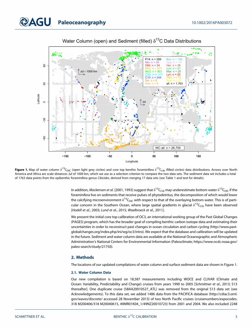
Figure 1. Map of water column δ13CDIC (open light grey circles) and core top benthic foraminifera δ13Ccib (filled circles) data distributions. Arrows over NorthAmerica and Africa are scale distances Δd of 1000 km, which we use as a selection criterion to compare the two data sets. The sediment data set includes a totalof 1763 data points from the epibenthic foraminifera genus Cibicides, derived from merging 17 data sets (see Table 1 and text for details).

Paleoceanography 10.1002/2016PA003072

SCHMITTNER ET AL. BENTHIC δ13C CALIBRATION 3

data from the earlier GEOSECS campaign (extracted from Ocean Data View on 21 September 2007)[Kroopnick, 1985], 639 observations from two recent GEOTRACES cruises, GI04 (205 data from the IndianOcean from year 2009) and GA03 (434 measurements from the North Atlantic from years 2010–2011)[Quay and Wu, 2015], 3339 data from the Atlantic and Indian Ocean sectors of the Southern Ocean from1989 to 2003 [Mackensen, 2012; M12 thereafter], 274 data from Arctic bottom waters from years 1990 to2008 [Mackensen, 2013; M13 thereafter], and 68 data from the southeastern margin of the Pacific[Martínez-Méndez et al., 2013]. The following 110 new (unpublished) measurements by Gema Martínez-Méndez were added as well: 60 data from the tropical West Pacific (Papua New Guinea: 14, Mindanao: 46),9 data from the southeast Pacific, 24 data from the subtropical northeast Atlantic, and 17 from thesubtropical South Atlantic. From the original M12 and M13 data sets 133 and 2 data were removed,respectively, because they included negative outliers, which were determined subjectively by inspectingindividual and multiple neighboring vertical profiles. Such outliers, which have been reported since theearly measurements of Kroopnick [1985], may be caused by contamination of the water samples. Fromthe original M13 data set we have also removed five data from the ODEN cruise and four data from theGEOSECS cruises because they are already included. In total the updated data set consists of 26,750individual observations, with broad spatial coverage, although large gaps remain in some regions such asthe eastern equatorial Atlantic, the South China Sea, and adjacent parts of the western tropical Pacific, andthe Indian and western Pacific sectors of the Southern Ocean (Figure 1). The S13 data set also includes dis-solved inorganic carbon (DIC) and alkalinity (ALK) observations, from which carbonate ion concentrations

Figure 2. Maps of (a) water depth, (b) observed carbonate ion concentration, (c) modeled anthropogenic δ13C correction (Δδ13Cant), and (d) observed temperature.Criteria of Δd = 1000 km, Δz = z/5 were used to map water column observations and model results.

Paleoceanography 10.1002/2016PA003072

SCHMITTNER ET AL. BENTHIC δ13C CALIBRATION 4

were approximated using the relationship [CO32�] ≅ ALK-DIC [Zeebe and Wolf-Gladrow, 2001], as well as

measurements of temperature (Figure 2d) and other variables. In case in situ [CO32�] or temperature was

not available we filled in climatological values from the Global Data Analysis Project [Key et al., 2004] andWorld Ocean Atlas 2005 [Locarnini et al., 2006].

Note that although not very well documented, δ13CDIC likely varies on seasonal to multicentennial and longertimescales. Therefore, the water column δ13CDIC data represent mostly snapshots in time of a temporally andspatially varying field. Generally, we can expect the temporal variations to be larger near the surface thanin the deep ocean. Temporal variability of δ13CDIC will therefore be a possible reason for offsets with thesediment data.

2.2. Surface Sediment Data

For our new compilation of foraminiferal measurements two types of data are included (Table 1 and Figure 1).

1. Sediment core top measurements of fossil foraminifera shells represent a long-term average covering theLate Holocene (LH; approximately the last 6000 years). The 1083 data from 15 data sets have beenassembled. Efforts to remove duplicates with already existing data were undertaken by manually sortingwith respect to depth and subsequent visual inspection of nearby entries with identical or similar latitude,longitude, and core name. Duplicates are excluded in the counts in Table 1. Many data sets do not providespecies information for individual data. For instance, P14 included records which the original authorsdescribed as “Cibs equivalent,” or “in equilibriumwith δ13CDIC,” but records listed as “mixed benthics”werenot included. Species information is currently available for a subset of 642 data, of which 550 areC. wuellerstorfi, 37 are C. kullenbergi, 12 are C. lobatulus, 34 are C. pachyderma, and 9 are C. floridanus.

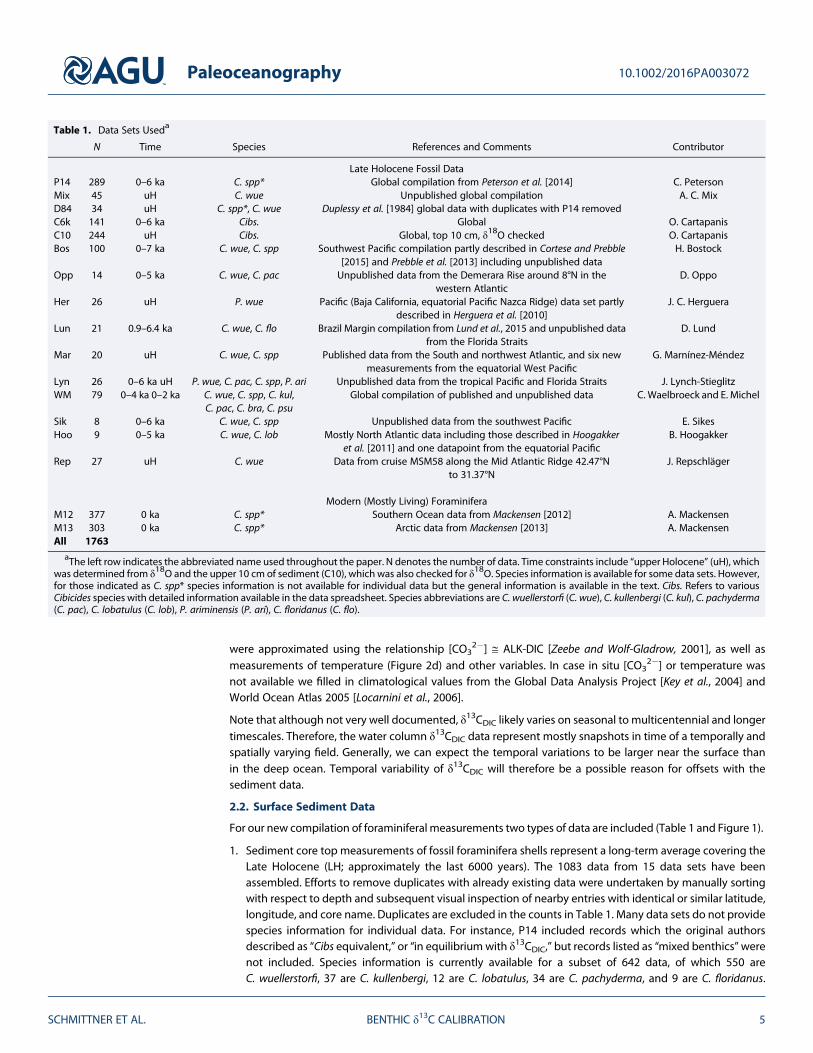
Table 1. Data Sets Useda

N Time Species References and Comments Contributor

Late Holocene Fossil DataP14 289 0–6 ka C. spp* Global compilation from Peterson et al. [2014] C. PetersonMix 45 uH C. wue Unpublished global compilation A. C. MixD84 34 uH C. spp*, C. wue Duplessy et al. [1984] global data with duplicates with P14 removedC6k 141 0–6 ka Cibs. Global O. CartapanisC10 244 uH Cibs. Global, top 10 cm, δ18O checked O. CartapanisBos 100 0–7 ka C. wue, C. spp Southwest Pacific compilation partly described in Cortese and Prebble

[2015] and Prebble et al. [2013] including unpublished dataH. Bostock

Opp 14 0–5 ka C. wue, C. pac Unpublished data from the Demerara Rise around 8°N in thewestern Atlantic

D. Oppo

Her 26 uH P. wue Pacific (Baja California, equatorial Pacific Nazca Ridge) data set partlydescribed in Herguera et al. [2010]

J. C. Herguera

Lun 21 0.9–6.4 ka C. wue, C. flo Brazil Margin compilation from Lund et al., 2015 and unpublished datafrom the Florida Straits

D. Lund

Mar 20 uH C. wue, C. spp Published data from the South and northwest Atlantic, and six newmeasurements from the equatorial West Pacific

G. Marnínez-Méndez

Lyn 26 0–6 ka uH P. wue, C. pac, C. spp, P. ari Unpublished data from the tropical Pacific and Florida Straits J. Lynch-StieglitzWM 79 0–4 ka 0–2 ka C. wue, C. spp, C. kul,

C. pac, C. bra, C. psuGlobal compilation of published and unpublished data C. Waelbroeck and E. Michel

Sik 8 0–6 ka C. wue, C. spp Unpublished data from the southwest Pacific E. SikesHoo 9 0–5 ka C. wue, C. lob Mostly North Atlantic data including those described in Hoogakker

et al. [2011] and one datapoint from the equatorial PacificB. Hoogakker

Rep 27 uH C. wue Data from cruise MSM58 along the Mid Atlantic Ridge 42.47°Nto 31.37°N

J. Repschläger

Modern (Mostly Living) ForaminiferaM12 377 0 ka C. spp* Southern Ocean data from Mackensen [2012] A. MackensenM13 303 0 ka C. spp* Arctic data from Mackensen [2013] A. MackensenAll 1763

aThe left row indicates the abbreviated name used throughout the paper. N denotes the number of data. Time constraints include “upper Holocene” (uH), whichwas determined from δ18O and the upper 10 cm of sediment (C10), which was also checked for δ18O. Species information is available for some data sets. However,for those indicated as C. spp* species information is not available for individual data but the general information is available in the text. Cibs. Refers to variousCibicides species with detailed information available in the data spreadsheet. Species abbreviations are C. wuellerstorfi (C. wue), C. kullenbergi (C. kul), C. pachyderma(C. pac), C. lobatulus (C. lob), P. ariminensis (P. ari), C. floridanus (C. flo).

Paleoceanography 10.1002/2016PA003072

SCHMITTNER ET AL. BENTHIC δ13C CALIBRATION 5

Despite this limited amount of information, we provide an initial analysis of species dependence. Sizeinformation is not always available either.

2. Measurements on modern, mostly living foraminifera, represent contemporary conditions but are limitedto high latitudes. Southern Ocean measurements cover years 1983 to 2001 (M12), and Arctic observa-tions are from 1987 to 2012 (M13). Each data point represents typically three shells, which is similar todowncore data, although the LH data may represent a larger number of shells since many of them wereaveraged over the last ~6 ka. M12 and M13 data sets are exclusively based on surface sediment samplestaken by large box or multiple corer. M12 and M13 used preferentially C. wuellerstorfi, and, where notavailable, Cibicides refulgens and C. lobatulus. In M12 also C. pachyderma, C. kullenbergi, and P. ariminensisare included.

The total number of data is 1763, approximately 28-fold more data than considered by D84. The sedimentdata span depths ranging from 64 m to 5691 m and all ocean basins (Figure 2a).

Note that the averaging period of the different data sets is different. The measurements on “living” foramini-fera represent a short, essentially instantaneous snapshot of the modern ocean. “Living” foraminifera aredefined as those stained by rose Bengal, but see, for instance, Bernhard et al. [2006] regarding vitality assess-ments of foraminifera using rose Bengal. In contrast, the LH core top data represent a heterogeneous assem-blage of long-term averages likely covering thousands of years (ka). P14, C6k, and Lyn use the last 6 ka, Bosuses the last 7 ka, and C10 uses the upper 10 cm of the sediment, whereas the averaging period for Mix, Rep,and D84 is simply defined as “upper Holocene” (uH) as determined from oxygen isotope values from thesame samples. Oxygen isotopes from the C10 data have been checked to make sure they represent lateHolocene conditions. Brazil Margin results (Lun), based on the uppermost sediment in each of the cores,which were radiocarbon dated between 900 to 6400 years BP, were preferred over longer time averages ofthe same cores included in any of the other data sets. Many of the core top samples analyzed are notprecisely dated. Some (in piston cores) may be contaminated by older material brought up by piston effects,or by overpenetration leading to the loss of the sediment water interface in the coring process. Data frommulticores that preserve pristine sediment-water interfaces are preferable and should be identified and com-pared to those from piston cores in future work. A limited, local comparison from the Florida Straits indicatesno systematic offsets, but differences of 0.1–0.2‰ between multicore and piston cores. For most sites,however, information on the coring equipment is not yet available in our database. Surface sediment datafrom box and multicores can also be contaminated by older sedimentary material at sites affected by erosionor winnowing. The only ways to exclude older material is via radiometric dating of the samples or comparisonof foraminifera oxygen isotope values with nearby cores.

2.3. Mapping Procedure

Water column and sediment data are generally not colocated. In order to map the water column data tothe sediment data, we use the horizontal great-circle distance (Δd) and the vertical distance (Δz) from thelocations (longitude, latitude, and depth) of the sediment data as a criterion. All water column data withinthose distances are averaged with equal weighting. Results are presented for two different choices: a moreliberal one (Δd = 1000 km, indicated in Figure 1, Δz = z/5), which will be the default, and a more conser-vative one (Δd = 500 km, Δz = z/10). The depth dependence for the vertical distance is motivated by thefact that like most other ocean tracer distributions, δ13CDIC shows larger vertical gradients in the upperocean than in the deep [Schmittner et al., 2013]. It leads to layer thicknesses of Δz = 100 m and 1 kmat depths of z = 500 m and 5 km, respectively, for the more liberal criterion and 50 m and 500 m, respec-tively, for the more conservative criterion. Mapped water column carbonate ion concentrations and tem-peratures are shown in Figure 2.

2.4. Anthropogenic Carbon

The invasion of 13C-depleted carbon into the upper ocean during the past century [Böhm et al., 2002] fromthe burning of fossil fuels has decreased δ13CDIC in the upper ocean during the past decades, a processknown as the Suess Effect [Gruber et al., 1999; Keeling, 1979; Suess, 1955]. Thus, some water column andmodern foraminiferal data have reduced δ13C values due to anthropogenic δ13CDIC (Δδ13Cant). The magni-tude of the offset varies depending on location and year the cores were collected. Hence, the Suess effectcould bias some comparisons to LH sediment data.

Paleoceanography 10.1002/2016PA003072

SCHMITTNER ET AL. BENTHIC δ13C CALIBRATION 6

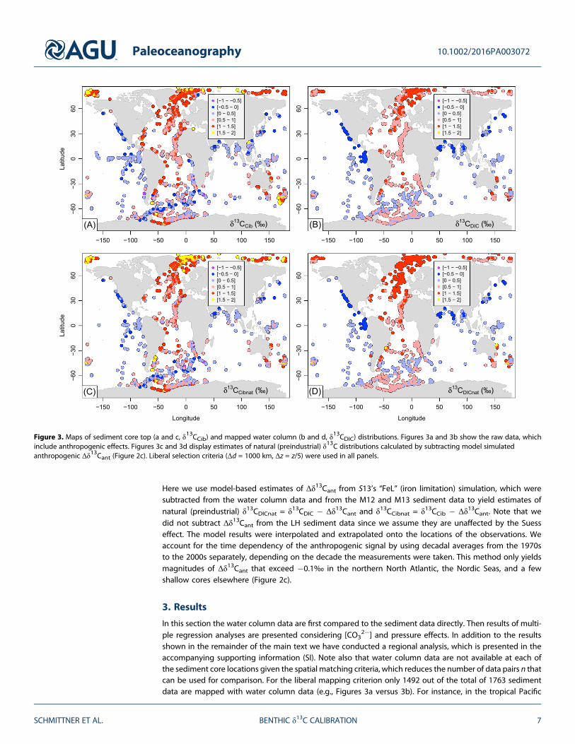
Here we use model-based estimates of Δδ13Cant from S13’s “FeL” (iron limitation) simulation, which weresubtracted from the water column data and from the M12 and M13 sediment data to yield estimates ofnatural (preindustrial) δ13CDICnat = δ13CDIC � Δδ13Cant and δ13CCibnat = δ13CCib � Δδ13Cant. Note that wedid not subtract Δδ13Cant from the LH sediment data since we assume they are unaffected by the Suesseffect. The model results were interpolated and extrapolated onto the locations of the observations. Weaccount for the time dependency of the anthropogenic signal by using decadal averages from the 1970sto the 2000s separately, depending on the decade the measurements were taken. This method only yieldsmagnitudes of Δδ13Cant that exceed �0.1‰ in the northern North Atlantic, the Nordic Seas, and a fewshallow cores elsewhere (Figure 2c).

3. Results

In this section the water column data are first compared to the sediment data directly. Then results of multi-ple regression analyses are presented considering [CO3

2�] and pressure effects. In addition to the resultsshown in the remainder of the main text we have conducted a regional analysis, which is presented in theaccompanying supporting information (SI). Note also that water column data are not available at each ofthe sediment core locations given the spatial matching criteria, which reduces the number of data pairs n thatcan be used for comparison. For the liberal mapping criterion only 1492 out of the total of 1763 sedimentdata are mapped with water column data (e.g., Figures 3a versus 3b). For instance, in the tropical Pacific

Figure 3. Maps of sediment core top (a and c, δ13CCib) and mapped water column (b and d, δ13CDIC) distributions. Figures 3a and 3b show the raw data, whichinclude anthropogenic effects. Figures 3c and 3d display estimates of natural (preindustrial) δ13C distributions calculated by subtracting model simulatedanthropogenic Δδ13Cant (Figure 2c). Liberal selection criteria (Δd = 1000 km, Δz = z/5) were used in all panels.

Paleoceanography 10.1002/2016PA003072

SCHMITTNER ET AL. BENTHIC δ13C CALIBRATION 7

around 140°W no water column data are available at the depth of the sediment data and within thehorizontal distance criterion. Similarly, in the eastern tropical Atlantic no water column data are availablefor comparison to the foraminifera data. Thus, our comparison is not only limited by the number ofsediment data but also by the sparse coverage of water column data. The amount of data available for themultiple linear regressions presented below is further reduced due to the limited availability of [CO3

2�]data such that for model LA1 in Table 2, only 1402 triplets of δ13CCibnat, δ

13CDICnat, and [CO32�] exist. For

the conservative mapping criteron these numbers are further reduced (see Tables 2 and 3).

3.1. Spatial Distributions of Sedimentary and Water Column Carbon Isotopes

The raw core top δ13CCib data vary from values of more than 1.9‰ in the Arctic and a few shallow cores fromelsewhere to less than �0.7‰ in the Atlantic sector of the Southern Ocean (Figure 3a). Atlantic values aremostly greater than 0.5‰, whereas in the Indian and Pacific Ocean they are mostly below 0.5‰, exceptfor some of the shallower sites. The water column δ13CDIC values mapped onto the sediment data displaysimilar interbasin differences, but the variations are much smoother (Figure 3b). Maximum values do not

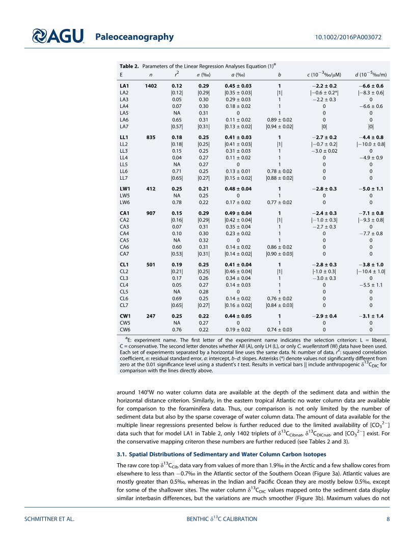
Table 2. Parameters of the Linear Regression Analyses Equation (1)a

E n r2 σ (‰) a (‰) b c (10�3‰/μM) d (10�5‰/m)

LA1 1402 0.12 0.29 0.45 ± 0.03 1 �2.2 ± 0.2 �6.6 ± 0.6LA2 |0.12| |0.29| |0.35 ± 0.03| |1| |�0.6 ± 0.2*| |�8.3 ± 0.6|LA3 0.05 0.30 0.29 ± 0.03 1 �2.2 ± 0.3 0LA4 0.07 0.30 0.18 ± 0.02 1 0 �6.6 ± 0.6LA5 NA 0.31 0 1 0 0LA6 0.65 0.31 0.11 ± 0.02 0.89 ± 0.02 0 0LA7 |0.57| |0.31| |0.13 ± 0.02| |0.94 ± 0.02| |0| |0|

LL1 835 0.18 0.25 0.41 ± 0.03 1 �2.7 ± 0.2 �4.4 ± 0.8LL2 |0.18| |0.25| |0.41 ± 0.03| |1| |�0.7 ± 0.2| |�10.0 ± 0.8|LL3 0.15 0.25 0.31 ± 0.03 1 �3.0 ± 0.02 0LL4 0.04 0.27 0.11 ± 0.02 1 0 �4.9 ± 0.9LL5 NA 0.27 0 1 0 0LL6 0.71 0.25 0.13 ± 0.01 0.78 ± 0.02 0 0LL7 |0.65| |0.27| |0.15 ± 0.02| |0.88 ± 0.02| 0 0

LW1 412 0.25 0.21 0.48 ± 0.04 1 �2.8 ± 0.3 �5.0 ± 1.1LW5 NA 0.25 0 1 0 0LW6 0.78 0.22 0.17 ± 0.02 0.77 ± 0.02 0 0

CA1 907 0.15 0.29 0.49 ± 0.04 1 �2.4 ± 0.3 �7.1 ± 0.8CA2 |0.16| |0.29| |0.42 ± 0.04| |1| |�1.0 ± 0.3| |�9.3 ± 0.8|CA3 0.07 0.31 0.35 ± 0.04 1 �2.7 ± 0.3 0CA4 0.10 0.30 0.23 ± 0.02 1 0 �7.7 ± 0.8CA5 NA 0.32 0 1 0 0CA6 0.60 0.31 0.14 ± 0.02 0.86 ± 0.02 0 0CA7 |0.53| |0.31| |0.14 ± 0.02| |0.90 ± 0.03| 0 0

CL1 501 0.19 0.25 0.41 ± 0.04 1 �2.8 ± 0.3 �3.8 ± 1.0CL2 |0.21| |0.25| |0.46 ± 0.04| |1| |-1.0 ± 0.3| |�10.4 ± 1.0|CL3 0.17 0.26 0.34 ± 0.04 1 �3.0 ± 0.3 0CL4 0.05 0.27 0.14 ± 0.03 1 0 �5.5 ± 1.1CL5 NA 0.28 0 1 0 0CL6 0.69 0.25 0.14 ± 0.02 0.76 ± 0.02 0 0CL7 |0.65| |0.27| |0.16 ± 0.02| |0.84 ± 0.03| 0 0

CW1 247 0.25 0.22 0.44 ± 0.05 1 �2.9 ± 0.4 �3.1 ± 1.4CW5 NA 0.27 0 1 0 0CW6 0.76 0.22 0.19 ± 0.02 0.74 ± 0.03 0 0

aE: experiment name. The first letter of the experiment name indicates the selection criterion: L = liberal,C = conservative. The second letter denotes whether All (A), only LH (L), or only C. wuellerstorfi (W) data have been used.Each set of experiments separated by a horizontal line uses the same data. N: number of data, r2: squared correlationcoefficient, σ: residual standard error, a: intercept, b–d: slopes. Asterisks (*) denote values not significantly different fromzero at the 0.01 significance level using a student’s t test. Results in vertical bars || include anthropogenic δ13CDIC forcomparison with the lines directly above.

Paleoceanography 10.1002/2016PA003072

SCHMITTNER ET AL. BENTHIC δ13C CALIBRATION 8

exceed 1.4‰, about 0.6‰ lower than those of the highest δ13CCib data. The lowest values of δ13CDIC (�0.5‰)

occur in the northern Indian and Pacific Oceans between about 1 and 2 km depth whereas the δ13CCibminima are found in the South Atlantic, where bottom water δ13CDIC is generally above 0‰. The standarddeviation of the sediment data of σ(δ13CCib) = 0.48‰ is higher than that of the water column dataσ(δ13CDIC) = 0.38‰.

Our estimates of δ13CCibnat (Figure 3c) are similar to the δ13CCib data except in the Arctic and subarctic NorthAtlantic and at a few shallow cores elsewhere, where the model predicts a substantial Suess effect (Figure 2c).Consequently, the water column δ13CDICnat estimates (Figure 3d) are higher than the δ13CDIC data in thoseregions. However, δ13CDIC data are affected by anthropogenic carbon in the deep midlatitude NorthAtlantic as far south as the subtropics, where most δ13CDICnat values are above 1‰. In contrast, not much dif-ference is seen between δ13CCibnat and δ13CCib there as a consequence of our assumption that the LH data donot need to be corrected for anthropogenic effects. These results are consistent with observational estimatesof intense uptake of anthropogenic carbon by deep water formation in the North Atlantic [Khatiwala et al.,2009; Olsen and Ninnemann, 2010]. Consistent with previous results [Schmittner et al., 2013], the standarddeviations of the preindustrial σ(δ13CCibnat) = 0.53‰ and σ(δ13CDICnat) = 0.47‰ are higher than those ofthe contemporary data, and, again, the sediment data have a larger standard deviation than the watercolumn data, which indicates that δ13CCib is influenced by additional processes than δ13CDIC.

The δ13CDICnat estimates in the deep ocean (~1500 to 3500 m) decrease along the flow path of deep waterfrom the North Atlantic south into the Southern Ocean and northward from the Southern Ocean into theIndian and Pacific oceans (Figures 4c and 4d). Along its path, water accumulates 13C-depleted carbon fromthe sinking and remineralization of organic matter which is the most important effect explaining the gradualdecrease in deep water δ13CDICnat from the Atlantic to the Pacific [Kroopnick, 1985; Schmittner et al., 2013]. In

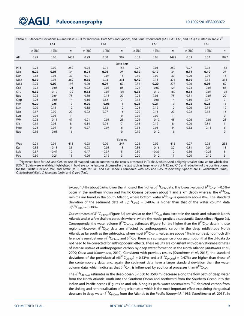
Table 3. Standard Deviations (σ) and Biases (�ε) for Individual Data Sets and Species, and Four Experiments (LA1, CA1, LA5, and CA5) as Listed in Table 2a

LA1 CA1 LA5 CA5

σ (‰) �ε (‰) n σ (‰) �ε (‰) n σ (‰) �ε (‰) n σ (‰) �ε (‰) n

All 0.29 0.00 1402 0.29 0.00 907 0.33 0.05 1492 0.33 0.07 1097

Data SetsP14 0.24 0.00 250 0.24 0.01 158 0.27 0.01 250 0.27 0.02 158Mix 0.22 0.05 34 0.24 0.05 25 0.32 0.17 34 0.34 0.19 25D84 0.18 0.01 30 0.21 �0.07 16 0.19 0.02 30 0.20 0.01 16M12 0.39 0.04 369 0.35 0.03 331 0.42 0.11 375 0.39 0.11 331M13 0.25 0.07 198 0.20 0.04 69 0.34 0.20 277 0.20 0.08 69C6k 0.22 �0.05 121 0.22 �0.05 85 0.24 �0.07 124 0.23 �0.08 85C10 0.32 �0.10 179 0.33 �0.08 108 0.33 �0.10 180 0.34 �0.07 108Bos 0.25 �0.04 75 0.30 �0.13 29 0.25 0.01 75 0.31 �0.08 29Opp 0.26 �0.05 14 0.16 0.12 7 0.18 �0.01 14 0.10 0.07 7Her 0.20 �0.01 19 0.20 �0.06 15 0.25 0.21 19 0.25 0.23 15Lun 0.20 0.11 12 0.18 0.13 12 0.21 0.12 12 0.20 0.14 12Mar 0.17 0.09 20 0.22 0.07 16 0.20 0.11 20 0.22 0.12 16Lyn 0.06 0.06 1 – – 0 0.09 0.09 1 – – 0WM 0.23 �0.11 47 0.21 �0.08 23 0.26 �0.10 48 0.26 �0.06 23Sik 0.12 0.05 8 0.14 0.04 7 0.16 0.12 8 0.20 0.51 1Hoo 0.28 0.04 9 0.27 �0.07 6 0.33 0.01 9 0.32 �0.13 6Rep 0.16 �0.03 16 – – 0 0.19 �0.12 16 – – 0

SpeciesWue 0.21 0.01 413 0.23 0.00 247 0.25 0.02 415 0.27 0.03 258Kul 0.35 �0.15 31 0.23 �0.08 13 0.36 �0.16 32 0.31 �0.04 15Lob 0.57 �0.47 12 0.47 �0.37 5 0.50 �0.39 12 0.36 �0.23 8Pac 0.30 �0.24 11 0.26 �0.16 3 0.20 �0.12 11 0.20 �0.12 3

aHowever, here for LA5 and CA5 we use all mapped data in contrast to the results presented in Table 2, which used a slightly smaller data set for which also[CO3

2�] data were available. Highlighted in bold are some features discussed in the text such as larger errors of M12 and C10 and reduction of the positive biasesfor the Pacific (Her and Mix) and Arctic (M13) data for LA1 and CA1 models compared with LA5 and CA5, respectively. Species are C. wuellerstorfi (Wue),C. kullenbergi (Kul), C. lobatulus (Lob), and C. pac (Pac).

Paleoceanography 10.1002/2016PA003072

SCHMITTNER ET AL. BENTHIC δ13C CALIBRATION 9

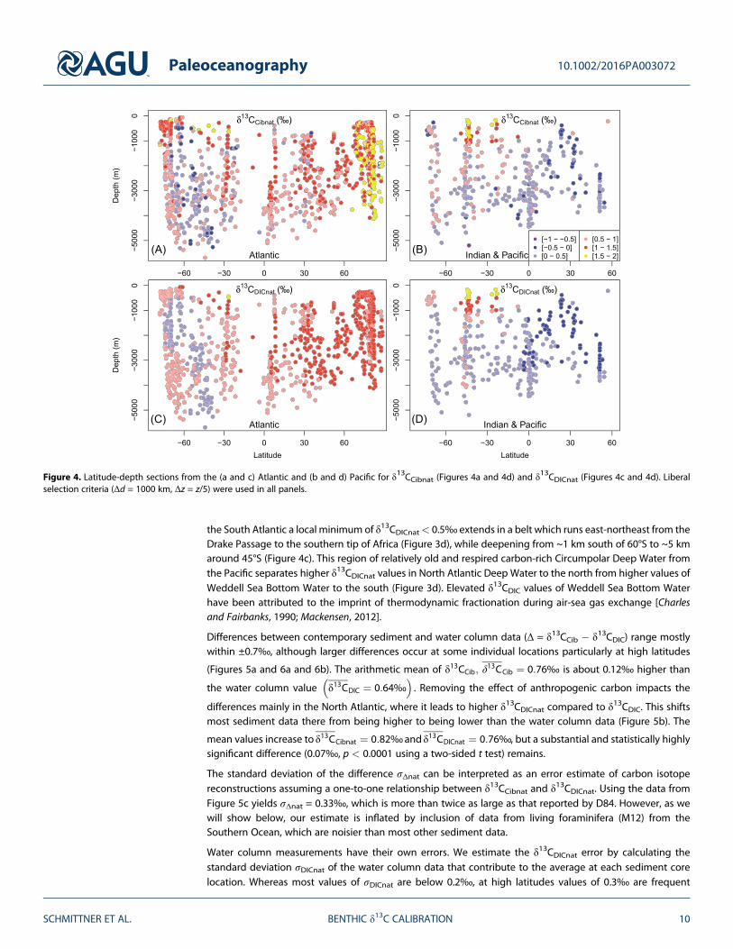
the South Atlantic a local minimum of δ13CDICnat< 0.5‰ extends in a belt which runs east-northeast from theDrake Passage to the southern tip of Africa (Figure 3d), while deepening from ~1 km south of 60°S to ~5 kmaround 45°S (Figure 4c). This region of relatively old and respired carbon-rich Circumpolar Deep Water fromthe Pacific separates higher δ13CDICnat values in North Atlantic Deep Water to the north from higher values ofWeddell Sea Bottom Water to the south (Figure 3d). Elevated δ13CDIC values of Weddell Sea Bottom Waterhave been attributed to the imprint of thermodynamic fractionation during air-sea gas exchange [Charlesand Fairbanks, 1990; Mackensen, 2012].

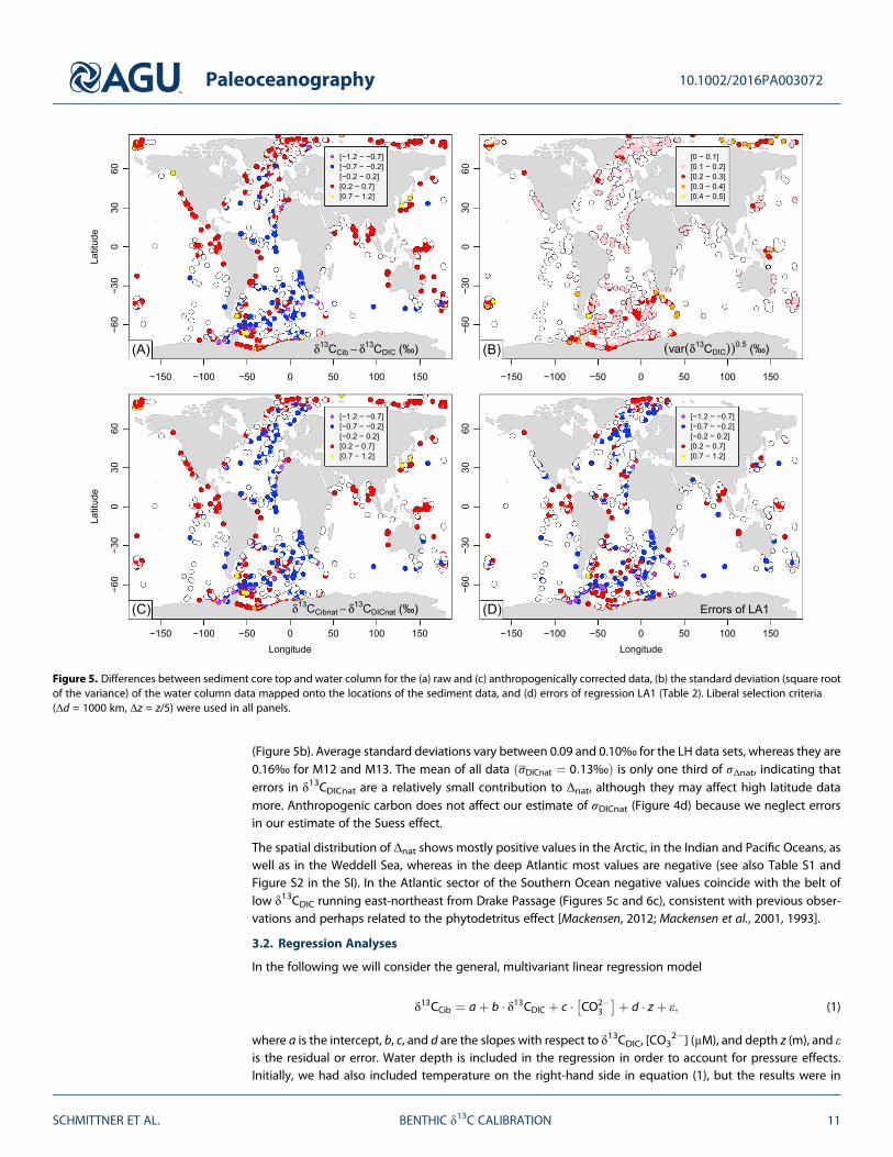
Differences between contemporary sediment and water column data (Δ = δ13CCib � δ13CDIC) range mostlywithin ±0.7‰, although larger differences occur at some individual locations particularly at high latitudes

(Figures 5a and 6a and 6b). The arithmetic mean of δ13CCib; δ13CCib ¼ 0:76‰ is about 0.12‰ higher than

the water column value δ13CDIC ¼ 0:64‰� �

. Removing the effect of anthropogenic carbon impacts the

differences mainly in the North Atlantic, where it leads to higher δ13CDICnat compared to δ13CDIC. This shiftsmost sediment data there from being higher to being lower than the water column data (Figure 5b). The

mean values increase to δ13CCibnat ¼ 0:82‰ and δ13CDICnat ¼ 0:76‰, but a substantial and statistically highlysignificant difference (0.07‰, p < 0.0001 using a two-sided t test) remains.

The standard deviation of the difference σΔnat can be interpreted as an error estimate of carbon isotopereconstructions assuming a one-to-one relationship between δ13CCibnat and δ13CDICnat. Using the data fromFigure 5c yields σΔnat = 0.33‰, which is more than twice as large as that reported by D84. However, as wewill show below, our estimate is inflated by inclusion of data from living foraminifera (M12) from theSouthern Ocean, which are noisier than most other sediment data.

Water column measurements have their own errors. We estimate the δ13CDICnat error by calculating thestandard deviation σDICnat of the water column data that contribute to the average at each sediment corelocation. Whereas most values of σDICnat are below 0.2‰, at high latitudes values of 0.3‰ are frequent

Figure 4. Latitude-depth sections from the (a and c) Atlantic and (b and d) Pacific for δ13CCibnat (Figures 4a and 4d) and δ13CDICnat (Figures 4c and 4d). Liberalselection criteria (Δd = 1000 km, Δz = z/5) were used in all panels.

Paleoceanography 10.1002/2016PA003072

SCHMITTNER ET AL. BENTHIC δ13C CALIBRATION 10

(Figure 5b). Average standard deviations vary between 0.09 and 0.10‰ for the LH data sets, whereas they are0.16‰ for M12 and M13. The mean of all data σDICnat ¼ 0:13‰ð Þ is only one third of σΔnat, indicating thaterrors in δ13CDICnat are a relatively small contribution to Δnat, although they may affect high latitude datamore. Anthropogenic carbon does not affect our estimate of σDICnat (Figure 4d) because we neglect errorsin our estimate of the Suess effect.

The spatial distribution of Δnat shows mostly positive values in the Arctic, in the Indian and Pacific Oceans, aswell as in the Weddell Sea, whereas in the deep Atlantic most values are negative (see also Table S1 andFigure S2 in the SI). In the Atlantic sector of the Southern Ocean negative values coincide with the belt oflow δ13CDIC running east-northeast from Drake Passage (Figures 5c and 6c), consistent with previous obser-vations and perhaps related to the phytodetritus effect [Mackensen, 2012; Mackensen et al., 2001, 1993].

3.2. Regression Analyses

In the following we will consider the general, multivariant linear regression model

δ13CCib ¼ aþ b � δ13CDIC þ c � CO2�3

� �þ d � z þ ε; (1)

where a is the intercept, b, c, and d are the slopes with respect to δ13CDIC, [CO32�] (μM), and depth z (m), and ε

is the residual or error. Water depth is included in the regression in order to account for pressure effects.Initially, we had also included temperature on the right-hand side in equation (1), but the results were in

Figure 5. Differences between sediment core top and water column for the (a) raw and (c) anthropogenically corrected data, (b) the standard deviation (square rootof the variance) of the water column data mapped onto the locations of the sediment data, and (d) errors of regression LA1 (Table 2). Liberal selection criteria(Δd = 1000 km, Δz = z/5) were used in all panels.

Paleoceanography 10.1002/2016PA003072

SCHMITTNER ET AL. BENTHIC δ13C CALIBRATION 11

many cases not statistically significant and resulted in inconsistent signs for the slopes depending on the datasets used (e.g., LH versus All). For these reasons we conclude that we do not find a consistent and statisticallysignificant temperature effect on δ13CCib and in the following we do not present results includingtemperature. Our default case used in most of our regression analyses will set b = 1 consistent with theory[Hesse et al., 2014] and because we are unaware of a δ13CDIC-dependent process that would affectfractionation during calcification or vital effects. On the other hand, we are aware and consider [CO3

2�]and pressure (depth)-dependent processes that produce offsets between δ13CCib and δ13CDIC by includingcoefficients c and d. In order to accommodate situations in which carbonate ion reconstructions are notavailable we will also consider cases with b ≠ 1. Since σΔ > σDIC, it is a reasonable first step to treat δ13CDICas the independent, error-free variable. We also assume that the errors associated with [CO3

2�] and z aresmall and treat them as independent variables.

The resulting statistical parameters including uncertainties are listed in Table 2 for six sets of sensitivityexperiments. The six sets differ according to data they include. The first three sets (LA1-LW6) use the liberalselection criterion (L), whereas the remaining three sets (CA1-CW6) use the conservative criterion (C). The firstand fourth sets (LA1-LA7 and CA1-CA7) use All data (A), whereas the second and fifth (LL1-LL7 and CL1-CL7)use LH data only (L), and the third and sixth set (LW1, LW5, and LW6 and CW1, CW5, and CW6) use C. wueller-storfi data only (W). Within a given set, up to seven experiments differ only in model assumptions. The firstexperiment in each set is the default marked in bold in Table 2. It includes carbonate ion and depth in theregression and assumes b = 1. Sensitivity experiments 2 and 7 evaluate the effects of not correcting foranthropogenic carbon. Sensitivity experiments 3 and 4 isolate the individual effects of [CO3

2�] and z, respec-tively, by only including one variable in the regression (c = 0 or d = 0). Experiment 5 represents the one-to-onerelationship (a = c = d = 0, b = 1). Experiments 6 and 7 allow for b ≠ 1. Statistical significance for all estimatedparameters is evaluated at the 0.01 significance level of the t statistic using the summary(lm) function in R.

All default experiments result in significant slopes c for carbonate ion concentrations ranging from �2.2 to�2.9 [10�3‰/(μmol kg�1)], with a mean of �2.6 ± 0.4 × 10�3‰/(μmol kg�1). Experiment 3 in each set,

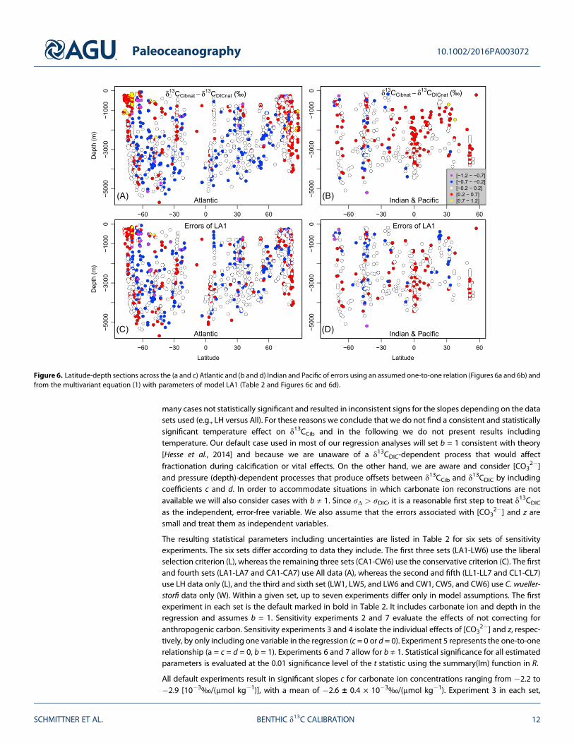
Figure 6. Latitude-depth sections across the (a and c) Atlantic and (b and d) Indian and Pacific of errors using an assumed one-to-one relation (Figures 6a and 6b) andfrom the multivariant equation (1) with parameters of model LA1 (Table 2 and Figures 6c and 6d).

Paleoceanography 10.1002/2016PA003072

SCHMITTNER ET AL. BENTHIC δ13C CALIBRATION 12

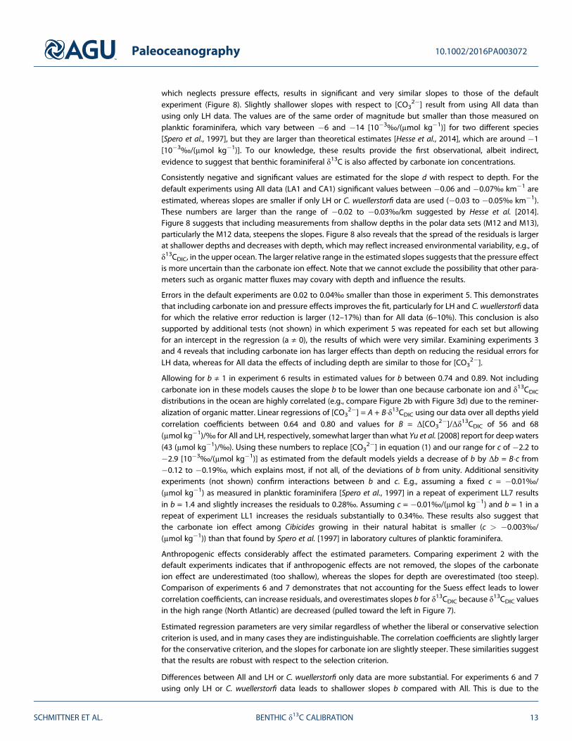
which neglects pressure effects, results in significant and very similar slopes to those of the defaultexperiment (Figure 8). Slightly shallower slopes with respect to [CO3

2�] result from using All data thanusing only LH data. The values are of the same order of magnitude but smaller than those measured onplanktic foraminifera, which vary between �6 and �14 [10�3‰/(μmol kg�1)] for two different species[Spero et al., 1997], but they are larger than theoretical estimates [Hesse et al., 2014], which are around �1[10�3‰/(μmol kg�1)]. To our knowledge, these results provide the first observational, albeit indirect,evidence to suggest that benthic foraminiferal δ13C is also affected by carbonate ion concentrations.

Consistently negative and significant values are estimated for the slope d with respect to depth. For thedefault experiments using All data (LA1 and CA1) significant values between �0.06 and �0.07‰ km�1 areestimated, whereas slopes are smaller if only LH or C. wuellerstorfi data are used (�0.03 to �0.05‰ km�1).These numbers are larger than the range of �0.02 to �0.03‰/km suggested by Hesse et al. [2014].Figure 8 suggests that including measurements from shallow depths in the polar data sets (M12 and M13),particularly the M12 data, steepens the slopes. Figure 8 also reveals that the spread of the residuals is largerat shallower depths and decreases with depth, which may reflect increased environmental variability, e.g., ofδ13CDIC, in the upper ocean. The larger relative range in the estimated slopes suggests that the pressure effectis more uncertain than the carbonate ion effect. Note that we cannot exclude the possibility that other para-meters such as organic matter fluxes may covary with depth and influence the results.

Errors in the default experiments are 0.02 to 0.04‰ smaller than those in experiment 5. This demonstratesthat including carbonate ion and pressure effects improves the fit, particularly for LH and C. wuellerstorfi datafor which the relative error reduction is larger (12–17%) than for All data (6–10%). This conclusion is alsosupported by additional tests (not shown) in which experiment 5 was repeated for each set but allowingfor an intercept in the regression (a ≠ 0), the results of which were very similar. Examining experiments 3and 4 reveals that including carbonate ion has larger effects than depth on reducing the residual errors forLH data, whereas for All data the effects of including depth are similar to those for [CO3

2�].

Allowing for b ≠ 1 in experiment 6 results in estimated values for b between 0.74 and 0.89. Not includingcarbonate ion in these models causes the slope b to be lower than one because carbonate ion and δ13CDICdistributions in the ocean are highly correlated (e.g., compare Figure 2b with Figure 3d) due to the reminer-alization of organic matter. Linear regressions of [CO3

2�] = A + B�δ13CDIC using our data over all depths yieldcorrelation coefficients between 0.64 and 0.80 and values for B = Δ[CO3

2�]/Δδ13CDIC of 56 and 68(μmol kg�1)/‰ for All and LH, respectively, somewhat larger than what Yu et al. [2008] report for deep waters(43 (μmol kg�1)/‰). Using these numbers to replace [CO3

2�] in equation (1) and our range for c of �2.2 to�2.9 [10�3‰/(μmol kg�1)] as estimated from the default models yields a decrease of b by Δb = B�c from�0.12 to �0.19‰, which explains most, if not all, of the deviations of b from unity. Additional sensitivityexperiments (not shown) confirm interactions between b and c. E.g., assuming a fixed c = �0.01‰/(μmol kg�1) as measured in planktic foraminifera [Spero et al., 1997] in a repeat of experiment LL7 resultsin b = 1.4 and slightly increases the residuals to 0.28‰. Assuming c = �0.01‰/(μmol kg�1) and b = 1 in arepeat of experiment LL1 increases the residuals substantially to 0.34‰. These results also suggest thatthe carbonate ion effect among Cibicides growing in their natural habitat is smaller (c > �0.003‰/(μmol kg�1)) than that found by Spero et al. [1997] in laboratory cultures of planktic foraminifera.

Anthropogenic effects considerably affect the estimated parameters. Comparing experiment 2 with thedefault experiments indicates that if anthropogenic effects are not removed, the slopes of the carbonateion effect are underestimated (too shallow), whereas the slopes for depth are overestimated (too steep).Comparison of experiments 6 and 7 demonstrates that not accounting for the Suess effect leads to lowercorrelation coefficients, can increase residuals, and overestimates slopes b for δ13CDIC because δ

13CDIC valuesin the high range (North Atlantic) are decreased (pulled toward the left in Figure 7).

Estimated regression parameters are very similar regardless of whether the liberal or conservative selectioncriterion is used, and in many cases they are indistinguishable. The correlation coefficients are slightly largerfor the conservative criterion, and the slopes for carbonate ion are slightly steeper. These similarities suggestthat the results are robust with respect to the selection criterion.

Differences between All and LH or C. wuellerstorfi only data are more substantial. For experiments 6 and 7using only LH or C. wuellerstorfi data leads to shallower slopes b compared with All. This is due to the

Paleoceanography 10.1002/2016PA003072

SCHMITTNER ET AL. BENTHIC δ13C CALIBRATION 13

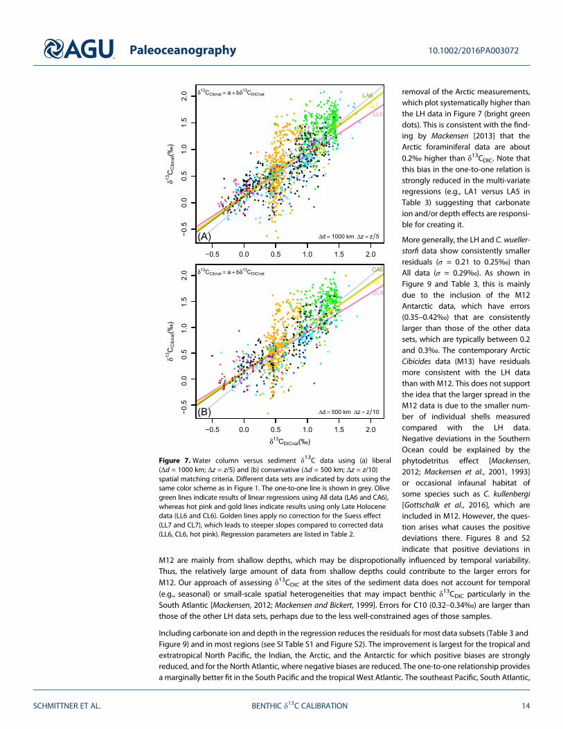
removal of the Arctic measurements,which plot systematically higher thanthe LH data in Figure 7 (bright greendots). This is consistent with the find-ing by Mackensen [2013] that theArctic foraminiferal data are about0.2‰ higher than δ13CDIC. Note thatthis bias in the one-to-one relation isstrongly reduced in the multi-variateregressions (e.g., LA1 versus LA5 inTable 3) suggesting that carbonateion and/or depth effects are responsi-ble for creating it.

More generally, the LH and C. wueller-storfi data show consistently smallerresiduals (σ = 0.21 to 0.25‰) thanAll data (σ = 0.29‰). As shown inFigure 9 and Table 3, this is mainlydue to the inclusion of the M12Antarctic data, which have errors(0.35–0.42‰) that are consistentlylarger than those of the other datasets, which are typically between 0.2and 0.3‰. The contemporary ArcticCibicides data (M13) have residualsmore consistent with the LH datathan with M12. This does not supportthe idea that the larger spread in theM12 data is due to the smaller num-ber of individual shells measuredcompared with the LH data.Negative deviations in the SouthernOcean could be explained by thephytodetritus effect [Mackensen,2012; Mackensen et al., 2001, 1993]or occasional infaunal habitat ofsome species such as C. kullenbergi[Gottschalk et al., 2016], which areincluded in M12. However, the ques-tion arises what causes the positivedeviations there. Figures 8 and S2indicate that positive deviations in

M12 are mainly from shallow depths, which may be dispropotionally influenced by temporal variability.Thus, the relatively large amount of data from shallow depths could contribute to the larger errors forM12. Our approach of assessing δ13CDIC at the sites of the sediment data does not account for temporal(e.g., seasonal) or small-scale spatial heterogeneities that may impact benthic δ13CDIC particularly in theSouth Atlantic [Mackensen, 2012; Mackensen and Bickert, 1999]. Errors for C10 (0.32–0.34‰) are larger thanthose of the other LH data sets, perhaps due to the less well-constrained ages of those samples.

Including carbonate ion and depth in the regression reduces the residuals for most data subsets (Table 3 andFigure 9) and in most regions (see SI Table S1 and Figure S2). The improvement is largest for the tropical andextratropical North Pacific, the Indian, the Arctic, and the Antarctic for which positive biases are stronglyreduced, and for the North Atlantic, where negative biases are reduced. The one-to-one relationship providesa marginally better fit in the South Pacific and the tropical West Atlantic. The southeast Pacific, South Atlantic,

Figure 7. Water column versus sediment δ13C data using (a) liberal(Δd = 1000 km; Δz = z/5) and (b) conservative (Δd = 500 km; Δz = z/10)spatial matching criteria. Different data sets are indicated by dots using thesame color scheme as in Figure 1. The one-to-one line is shown in grey. Olivegreen lines indicate results of linear regressions using All data (LA6 and CA6),whereas hot pink and gold lines indicate results using only Late Holocenedata (LL6 and CL6). Golden lines apply no correction for the Suess effect(LL7 and CL7), which leads to steeper slopes compared to corrected data(LL6, CL6, hot pink). Regression parameters are listed in Table 2.

Paleoceanography 10.1002/2016PA003072

SCHMITTNER ET AL. BENTHIC δ13C CALIBRATION 14

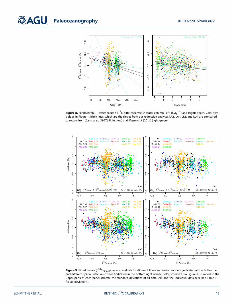
Figure 8. Foraminifera � water column δ13C difference versus water column (left) [CO32�] and (right) depth. Color sym-

bols as in Figure 1. Black lines, which are the slopes from our regression analyses LA3, LA4, LL3, and LL4, are comparedto results from Spero et al. [1997] (light blue) and Hesse et al. [2014] (light green).

Figure 9. Fitted values (δ13CCibnat) versus residuals for different linear regression models (indicated at the bottom left)and different spatial selection criteria (indicated in the bottom right corner. Color scheme as in Figure 1. Numbers in theupper parts of each panel indicate the standard deviations of all data (All) and the individual data sets (see Table 1for abbreviations).

Paleoceanography 10.1002/2016PA003072

SCHMITTNER ET AL. BENTHIC δ13C CALIBRATION 15

and Antarctic are the regions withthe largest errors for model LA1(Table S1). Not many data are avail-able from the southeast Pacific,hampering the assessment there.

The South Atlantic shows interest-ing zonal differences. Errors arelarger in the southeast Atlanticwhere foraminifera-based esti-mates suffer from a substantialnegative bias of �0.18‰, whereasin the southwest Atlantic their biasis smaller and positive (+0.07‰).Note that these biases exacerbatethe zonal difference from lessthan 0.2‰ in the water columnto more than 0.4‰ in theforminifera-based estimates.

Using the more conservative spa-tial matching criteria reduces theresiduals in some cases (M13 andOpp), which indicates that errorsin δ13CDIC do affect the results,but the overall effect appears tobe relatively small.

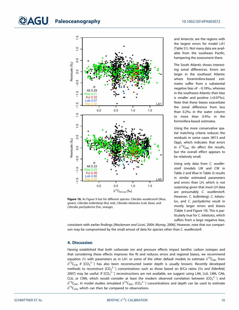
Using only data from C. wueller-storfi (models LW and CW inTable 2 and Wue in Table 3) resultsin similar estimated parametersand errors than LH, which is notsurprising given that most LH dataare presumably C. wuellerstorfi.However, C. kullenbergi, C. lobatu-lus, and C. pachyderma result inmostly larger errors and biases(Table 3 and Figure 10). This is par-ticularly true for C. lobatulus, whichsuffers from a large negative bias,

consistent with earlier findings [Mackensen and Licari, 2004; Murray, 2006]. However, note that our compari-son may be compromised by the small amout of data for species other than C. wuellerstorfi.

4. Discussion

Having established that both carbonate ion and pressure effects impact benthic carbon isotopes andthat considering these effects improves the fit and reduces errors and regional biases, we recommendequation (1) with parameters as in LA1 or some of the other default models to estimate δ13CDIC fromδ13CCib if [CO3

2�] has also been reconstructed (water depth is usually known). Recently developedmethods to reconstruct [CO3

2�] concentrations such as those based on B/Ca ratios [Yu and Elderfield,2007] may be useful. If [CO3

2�] reconstructions are not available, we suggest using LA6, LL6, LW6, CA6,CL6, or CW6, which would consider at least the modern observed correlation between [CO3

2�] andδ13CDIC. In model studies simulated δ13CDIC, [CO3

2�] concentrations and depth can be used to estimateδ13CCib, which can then be compared to observations.

Figure 10. As Figure 9 but for different species: Cibicides wuellerstorfi (Wue,green), Cibicides kullenbergi (Kul, red), Cibicides lobatulus (Lob, blue), andCibicides pachyderma (Pac, orange).

Paleoceanography 10.1002/2016PA003072

SCHMITTNER ET AL. BENTHIC δ13C CALIBRATION 16

Implications of pH and temperature effects on glacial-interglacial δ13CDIC reconstructions have been dis-cussed previously in Hesse et al. [2014] who found a strong temperature effect that suggests that 0.11‰ ofthe observed total whole ocean ~0.35‰ δ13CCib drop from the interglacial to the glacial ocean could beexplained by a cooling of bottom waters by 2.5°C. Our analysis did not result in a consistent significanttemperature effect, thus questioning their conclusion.

Our results have implications for glacial-interglacial δ13C reconstructions. Carbonate ion concentrationswere similar in the Pacific and Indian oceans but about 20 μmol kg�1 lower in the deep Atlantic and 20 to30 μmol kg�1 higher in the upper Atlantic during the LGM compared to the preindustrial ocean [Allen et al.,2015; Gottschalk et al., 2015; Yu et al., 2008, 2013, 2014]. Using equation (1) with c = �2.6 × 10�3‰/(μmol kg�1), this would produce a 0.05‰ reduction in δ13CDIC in the deep Atlantic and an increase of0.05–0.08‰ in the upper Atlantic, thereby slightly enhancing the observed interglacial-to-glacial increasein the vertical gradient of ~1.0‰ in δ13CCib [Yu et al., 2008, Figure 4].

Our finding that biases in the South Atlantic exacerbate the zonal gradient in δ13CDIC there may also explainthe large zonal gradients found in glacial reconstructions there [Hodell et al., 2003; Hoffman and Lund, 2012;Waelbroeck et al., 2011] and questions their reliability, particularly those from the southeast Atlantic whereδ13CCib exhibits large negative biases compared with δ13CDIC regardless of whether carbonate ion and pres-sure effects are considered or not (Table S1). The ultimate reasons for these biases as well as the large errors inthe Antarctic remain open questions.

Remaining errors may be influenced by accumulation rates. In low accumulation rate cores, bioturbationmay cause contamination of surface sediments with older glacial or deglacial material. Currently, accu-mulation rate information is not available in our data set, but it would be desirable to include it inthe future in order to evaluate this issue. Future updates of the database with more consistent species,core top dating, and coring equipment information and analyzing if and how residuals are affected willbe another useful effort.

5. Summary and Conclusions

Our synthesis of late Holocene core top δ13CCib data includes more than an order of magnitude more mea-surements than that used in the previous global calibration of D84. This, together with the vastly enhanceddatabase of water column δ13CDIC measurements, has prompted a new global calibration of δ13CCib. Theresults confirm the strong correlation between δ13CCib and δ13CDIC found by D84. However, we show thatresults of regression analyses are impacted by the invasion of 13C-depleted, anthropogenic carbon and indi-cate statistically significant secondary effects from carbonate ion and pressure. Including these secondaryeffects improves the estimation of δ13CDIC by reducing systematic regional biases, errors and by increasingcorrelation. We therefore recommend using equation (1) with parameters LA1 (Table 2) rather than a simpleone-to-one relationship between δ13CDIC ≈ δ13CCib. The regression coefficients with respect to carbonate ionand pressure are qualitatively consistent with previous theoretical [Hesse et al., 2014] and experimental [Speroet al., 1997] studies, but quantitatively, the carbonate ion effects are smaller than those of Spero et al. [1997]and larger than those of Hesse et al. [2014], respectively. Hence, these secondary effects are relatively smalland would in practical applications modify reconstructed δ13CDIC changes by typically less than about 15%compared to the often used one-to-one relationship. For most individual downcore records, z is practicallyinvariant and carbonate ion varies relatively little, so that they will have limited impact on reconstructionsof temporal variability. Thus, most conclusions of previous studies assuming a one-to-one relationship remainlikely robust.

We find errors are typically 0.2–0.3‰, although they are larger in the southeast Atlantic and Antarctic(~0.4‰) and larger in the upper ocean than at depths. We find lower errors for C. wuellerstorfi and highererrors and negative biases for C. lobatulus compared with C. kullenbergi and C. pachyderma, consistent withMackensen and Licari [2004] and Murray [2006] who also indicate lower δ13C values for C. lobatulus. Theseerrors are larger than the 0.15‰ reported by D84. Future efforts could be directed toward understandingthe sources for the remaining errors, such as a more comprehensive analysis of species offsets, informationon size and number of shells measured, coring equipment used, sediment type and accumulation rates,age constraints, and temporal variability of δ13CDIC and δ13CCib, so as to be able to improve the use of δ13C

Paleoceanography 10.1002/2016PA003072

SCHMITTNER ET AL. BENTHIC δ13C CALIBRATION 17

as a paleoceanographic proxy. This will require updating and extending the database to include relevant butcurrently missing information.

ReferencesAllen, K. A., E. L. Sikes, B. Honisch, A. C. Elmore, T. P. Guilderson, Y. Rosenthal, and R. F. Anderson (2015), Southwest Pacific deep water

carbonate chemistry linked to high southern latitude climate and atmospheric CO2 during the Last Glacial Termination, Quat. Sci. Rev.,122, 180–191.

Belanger, P. E., W. B. Curry, and R. K. Matthews (1981), Core-top evaluation of benthic foraminiferal isotopic-ratios for paleo-oceanographicinterpretations, Palaeogeogr. Palaeoclimatol. Palaeoecol., 33, 205–220.

Bernhard, J. M., D. R. Ostermann, D. S. Williams, and J. K. Blanks (2006), Comparison of two methods to identify live benthic foraminifera: Atest between Rose Bengal and CellTracker Green with implications for stable isotope paleoreconstructions, Paleoceanography, 21,PA4210, doi:10.1029/2006PA001290.

Böhm, F., A. Haase-Schramm, A. Eisenhauer, W. C. Dullo, M. M. Joachimski, H. Lehnert, and J. Reitner (2002), Evidence for preindustrialvariations in the marine surface water carbonate system from coralline sponges, Geochem. Geophys. Geosyst., 3(3), doi:10.1029/2001GC000264.

Broecker, W. S. (1982), Glacial to interglacial changes in ocean chemistry, Prog. Oceanogr., 11, 151–197.Charles, C. D., and R. G. Fairbanks (1990), Glacial to interglacial changes in the isotopic gradients of Southern Ocean surface water, in

Geological History of the Polar Oceans: Arctic Versus Antarctic, edited by U. Bleil and J. Thiede, pp. 519–538, Springer, Netherlands.Corliss, B. H. (1985), Microhabitats of benthic foraminifera within deep-sea sediments, Nature, 314, 435–438.Cortese, G., and J. Prebble (2015), A radiolarian-based modern analogue dataset for palaeoenvironmental reconstructions in the southwest

Pacific, Mar. Micropaleontol., 118, 34–49.Curry, W. B., and D. W. Oppo (2005), Glacial water mass geometry and the distribution of delta C-13 of Sigma CO2 in the western Atlantic

Ocean, Paleoceanography, 20, PA1017, doi:10.1029/2004PA001021.Duplessy, J. C., N. J. Shackleton, R. K. Matthews, W. Prell, W. F. Ruddiman, M. Caralp, and C. H. Hendy (1984), C-13 record of benthic forami-

nifera in the last interglacial ocean—Implications for the carbon-cycle and the global deep-water circulation, Quat. Res., 21, 225–243.Duplessy, J. C., N. J. Shackleton, R. G. Fairbanks, L. Labeyrie, D. Oppo, and N. Kallel (1988), Deepwater source variations during the last climatic

cycle and their impact on the global deepwater circulation, Paleoceanography, 3, 343–360.Fontanier, C., A. Mackensen, F. J. Jorissen, P. Anschutz, L. Licari, and C. Griveaud (2006), Stable oxygen and carbon isotopes of live benthic

foraminifera from the Bay of Biscay: Microhabitat impact and seasonal variability, Mar. Micropaleontol., 58, 159–183.Gebbie, G. (2014), How much did glacial North Atlantic water shoal?, Paleoceanography, 29, 190–209, doi:10.1002/2013PA002557.Gottschalk, J., L. C. Skinner, S. Misra, C. Waelbroeck, L. Menviel, and A. Timmermann (2015), Abrupt changes in the southern extent of North

Atlantic Deep Water during Dansgaard-Oeschger events, Nat. Geosci., 8, 950–U986.Gottschalk, J., N. Vázquez Riveiros, C. Waelbroeck, L. C. Skinner, E. Michel, J. C. Duplessy, D. A. Hodell, and A. Mackensen (2016), Carbon

isotope offsets between benthic foraminifer species of the genus Cibicides (Cibicidoides) in the glacial sub-Antarctic Atlantic,Paleoceanography, 31, 1583–1602, doi:10.1002/2016PA003029.

Gruber, N., C. D. Keeling, R. B. Bacastow, P. R. Guenther, T. J. Lueker, M. Wahlen, H. A. J. Meijer, W. G. Mook, and T. F. Stocker (1999),Spatiotemporal patterns of carbon-13 in the global surface oceans and the oceanic Suess effect, Global Biogeochem. Cycles, 13,307–335.

Herguera, J. C., T. Herbert, M. Kashgarian, and C. Charles (2010), Intermediate and deep water mass distribution in the Pacific during the LastGlacial Maximum inferred from oxygen and carbon stable isotopes, Quat. Sci. Rev., 29, 1228–1245.

Hesse, T., D. Wolf-Gladrow, G. Lohmann, J. Bijma, A. Mackensen, and R. E. Zeebe (2014), Modelling delta C-13 in benthic foraminifera: Insightsfrom model sensitivity experiments, Mar. Micropaleontol., 112, 50–61.

Hodell, D. A., C. D. Charles, and F. J. Sierro (2001), Late Pleistocene evolution of the ocean’s carbonate system, Earth Planet. Sci. Lett., 192,109–124.

Hodell, D. A., K. A. Venz, C. D. Charles, and U. S. Ninnemann (2003), Pleistocene vertical carbon isotope and carbonate gradients in the SouthAtlantic sector of the Southern Ocean, Geochem. Geophys. Geosyst., 4(1), 1004, doi:10.1029/2002GC000367.

Hoffman, J. L., and D. C. Lund (2012), Refining the stable isotope budget for Antarctic BottomWater: New foraminiferal data from the abyssalSouthwest Atlantic, Paleoceanography, 27, PA1213, doi:10.1029/2011PA002216.

Hoogakker, B. A. A., M. R. Chapman, I. N. McCave, C. Hillaire-Marcel, C. R. W. Ellison, I. R. Hall, and R. J. Telford (2011), Dynamics of North Atlanticdeep water masses during the holocene, Paleoceanography, 26, PA4214, doi:10.1029/2011PA002155.

Ishimura, T., U. Tsunogai, S. Hasegawa, S. Hasegawa, T. Oi, H. Kitazato, H. Suga, and T. Toyofuku (2012), Variation in stable carbon andoxygen isotopes of individual benthic foraminifera: Tracers for quantifying the magnitude of isotopic disequilibrium, Biogeosciences, 9,4353–4367.

Jorissen, F. J., H. C. de Stigter, and J. G. V. Widmark (1995), A conceptual model explaining benthic foraminiferal microhabitats,Mar. Micropaleontol., 26, 3–15.

Keeling, C. D. (1979), The Suess effect:13Carbon-

14Carbon interrelations, Environ. Int., 2, 229–300.

Key, R. M., A. Kozyr, C. L. Sabine, K. Lee, R. Wanninkhof, J. L. Bullister, R. A. Feely, F. J. Millero, C. Mordy, and T.-H. Peng (2004), A global oceancarbon climatology: Results from global data analysis project (GLODAP), Global Biogeochem. Cycles, 18, GB4031, doi:10.1029/2004GB002247.

Khatiwala, S., F. Primeau, and T. Hall (2009), Reconstruction of the history of anthropogenic CO2 concentrations in the ocean, Nature, 462,346–U110.

Kroopnick, P. M. (1985), The distribution of C-13 of Sigma-CO2 in the World oceans, Deep Sea Res., Part A, 32, 57–84.Locarnini, R. A., A. V. Mishonov, J. I. Antonov, T. P. Boyer, and H. E. Garcia (2006),World Ocean Atlas 2005, Volume 1: Temperature, NOAA Atlas

NESDIS 61, edited by S. Levitus, pp. 1–182, U.S. Gov. Print. Off., Washington, D. C.Lund, D. C., A. C. Tessin, J. L. Hoffman, and A. Schmittner (2015), Southwest Atlantic watermass evolution during the last deglaciation,

Paleoceanography, 30, 477–494, doi:10.1002/2014PA002657.Lutze, G. F., and H. Thiel (1989), Epibenthic foraminifera from elevated microhabitats; Cibicidoides wuellerstorfi and Planulina ariminensis,

J. Foramin. Res., 19, 153.Lynch-Stieglitz, J., M. W. Schmidt, L. Gene Henry, W. B. Curry, L. C. Skinner, S. Mulitza, R. Zhang, and P. Chang (2014), Muted change in Atlantic

overturning circulation over some glacial-aged Heinrich events, Nat. Geosci., 7, 144–150.

Paleoceanography 10.1002/2016PA003072

SCHMITTNER ET AL. BENTHIC δ13C CALIBRATION 18

AcknowledgmentsWe thank Matthew P. Humphreys fornoting a duplicate cruise in the S13 dataset, which we subsequently removed.OC3 is supported by PAGES, a coreproject of Future Earth. PAGES issupported by the U.S. and SwissNational Science Foundations. Supportfor this project was also provided by theU.S. National Science Foundation(award 1634719 to A.S. and A.C.M.,awards 0926735 and 1125181 to L.E.L.and C.D.P., and award OCE-1003500 toD.C.L.), the Swiss National ScienceFoundation (awards PP00P2_144811and 200021_163003 to S.L.J.), theCanadian Institute for AdvancedResearch (CIFAR), the CanadianFoundation for Innovation (CFI), and theNatural Sciences and EngineeringResearch Council (NSERC). Authors ofnewly presented data in this paperexpress their gratitude to the variousship expedition parties and chiefscientists for making material available(SO228, SO245, MSM48, and M124).Data used are listed in the references,tables, and supplements and availableat NOAA’s Paleoclimate repository athttps://www.ncdc.noaa.gov/paleo-search/study/21750 (water columndata) and https://www.ncdc.noaa.gov/paleo-search/study/22110 (sedimentcore top data).

Mackensen, A. (2012), Strong thermodynamic imprint on recent bottom-water and epibenthic delta C-13 in the Weddell Sea revealed:Implications for glacial Southern Ocean ventilation, Earth Planet. Sci. Lett., 317, 20–26.

Mackensen, A. (2013), High epibenthic foraminiferal delta C-13 in the recent deep Arctic Ocean: Implications for ventilation and brine releaseduring stadials, Paleoceanography, 28, 574–584, doi:10.1002/palo.20058.

Mackensen, A., and T. Bickert (1999), Stable carbon isotopes in benthic foraminifera: Proxies for deep and bottom water circulation and newproduction, in Use of Proxies in Paleoceanography: Examples From the South Atlantic, edited by G. Fischer and G. Wefer, pp. 229–254,Springer, Berlin, Heidelberg.

Mackensen, A., and L. Licari (2004), Carbon isotopes of live benthic foraminifera from the South Atlantic: Sensitivity to bottom watercarbonate saturation state and organic matter rain rates, in The South Atlantic in the Late Quaternary, edited by G. Wefer, S. Mulitza, andV. Ratmeyer, pp. 623–644, Springer, Berlin, Heidelberg.

Mackensen, A., H. W. Hubberten, T. Bickert, G. Fischer, and D. K. Fuetterer (1993), The δ13C in benthic foraminiferal tests of Fontbotiawuellerstorfi (Schwager) relative to the δ13C of dissolved inorganic carbon in Southern Ocean Deep Water: Implications for glacial oceancirculation models, Paleoceanography, 8, 587–610.

Mackensen, A., M. Rudolph, and G. Kuhn (2001), Late Pleistocene deep-water circulation in the subantarctic eastern Atlantic, Global Planet.Change, 30, 197–229.

Marchal, O., and W. B. Curry (2008), On the abyssal circulation in the glacial Atlantic, J. Phys. Oceanogr., 38, 2014–2037.Martínez-Méndez, G., D. Hebbeln, M. Mohtadi, F. Lamy, R. D. Pol-Holz, D. Reyes-Macaya, and T. Freudenthal (2013), Changes in the advection

of Antarctic Intermediate Water to the northern Chilean coast during the last 970 kyr, Paleoceanography, 28, 607–618, doi:10.1002/palo.20047.

McCorkle, D. C., S. R. Emerson, and P. D. Quay (1985), Stable carbon isotopes in marine porewaters, Earth Planet. Sci. Lett., 74, 13–26.McCorkle, D. C., L. D. Keigwin, B. H. Corliss, and S. R. Emerson (1990), The influence of microhabitats on the carbon isotopic composition of

deep-sea benthic foraminifera, Paleoceanography, 5, 161–185.Murray, J. W. (2006), Ecology and Applications of Benthic Foraminifera, pp. 1–426, Cambridge Univ. Press, Cambridge, U. K.Olsen, A., and U. Ninnemann (2010), Large delta C-13 gradients in the preindustrial North Atlantic revealed, Science, 330, 658–659.Peterson, C. D., L. E. Lisiecki, and J. V. Stern (2014), Deglacial whole-ocean delta C-13 change estimated from 480 benthic foraminiferal

records, Paleoceanography, 29, 549–563, doi:10.1002/2013PA002552.Prebble, J. G., E. M. Crouch, L. Carter, G. Cortese, H. Bostock, and H. Neil (2013), An expanded modern dinoflagellate cyst dataset for the

Southwest Pacific and Southern Hemisphere with environmental associations, Mar. Micropaleontol., 101, 33–48.Quay, P., and J. Wu (2015), Impact of end-member mixing on depth distributions of δ

13C, cadmium and nutrients in the N. Atlantic Ocean,

Deep Sea Res., Part II, 116, 107–116.Rathburn, A. E., B. H. Corliss, K. D. Tappa, and K. C. Lohmann (1996), Comparisons of the ecology and stable isotopic compositions of living

(stained) benthic foraminifera from the Sulu and South China Seas, Deep Sea Res., Part I, 43, 1617–1646.Schmiedl, G., M. Pfeilsticker, C. Hemleben, and A. Mackensen (2004), Environmental and biological effects on the stable isotope composition

of recent deep-sea benthic foraminifera from the western Mediterranean Sea, Mar. Micropaleontol., 51, 129–152.Schmittner, A., N. Gruber, A. C. Mix, R. M. Key, A. Tagliabue, and T. K. Westberry (2013), Biology and air-sea gas exchange controls on the

distribution of carbon isotope ratios (δ13C) in the ocean, Biogeosciences, 10, 5793–5816.

Schweizer, M., J. Pawlowski, T. Kouwenhoven, and B. van der Zwaan (2009), Molecular phylogeny of common cibicidids and related rotaliida(foraminifera) based on small subunit rDNA sequences, J. Foraminifer. Res., 39, 300.

Shackleton, N. J. (1977), Carbon-13 in Uvigerina: Tropical rainforest history and the Equatorial Pacific carbonate dissolution cycles, in The Fateof Fossil Fuel CO2 in the Oceans, edited by N. R. Andersen, and A. Malahoff, pp. 401–427, Plenum, New York.

Spero, H. J., J. Bijma, D. W. Lea, and B. E. Bemis (1997), Effect of seawater carbonate concentration on foraminiferal carbon and oxygenisotopes, Nature, 390, 497–500.

Suess, H. E. (1955), Radiocarbon concentration in modern wood, Science, 122, 415.Tachikawa, K., and H. Elderfield (2002), Microhabitat effects on Cd/Ca and delta C-13 of benthic foraminifera, Earth Planet. Sci. Lett., 202,

607–624.Waelbroeck, C., C. Skinner, L. Labeyrie, J.-C. Duplessy, E. Michel, N. Vazquez Riveiros, J.-M. Gherardi, and F. Dewilde (2011), The timing of

deglacial circulation changes in the Atlantic, Paleoceanography, 26, PA3213, doi:10.1029/2010PA002007.Weinelt, M., et al. (2001), Paleoceanographic proxies in the northern North Atlantic, in The Northern North Atlantic: A Changing Environment,

edited by P. Schäfer et al., pp. 319–352, Springer, Berlin, Heidelberg.Wollenburg, J. E., M. Raitzsch, and R. Tiedemann (2015), Novel high-pressure culture experiments on deep-sea benthic foraminifera—

Evidence for methane seepage-related δ13C of Cibicides wuellerstorfi, Mar. Micropaleontol., 117, 47–64.

Yu, J. M., and H. Elderfield (2007), Benthic foraminiferal B/Ca ratios reflect deep water carbonate saturation state, Earth Planet. Sci. Lett., 258,73–86.

Yu, J. M., H. Elderfield, and A. M. Piotrowski (2008), Seawater carbonate ion-delta C-13 systematics and application to glacial-interglacialNorth Atlantic ocean circulation, Earth Planet. Sci. Lett., 271, 209–220.

Yu, J. M., R. F. Anderson, Z. D. Jin, J. W. B. Rae, B. N. Opdyke, and S. M. Eggins (2013), Responses of the deep ocean carbonate system to carbonreorganization during the Last Glacial–interglacial cycle, Quat. Sci. Rev., 76, 39–52.

Yu, J. M., R. F. Anderson, Z. D. Jin, L. Menviel, F. Zhang, F. J. Ryerson, and E. J. Rohling (2014), Deep South Atlantic carbonate chemistry andincreased interocean deep water exchange during last deglaciation, Quat. Sci. Rev., 90, 80–89.

Zahn, R., K. Winn, and M. Sarnthein (1986), Benthic foraminiferal δ13C and accumulation rates of organic carbon: Uvigerina peregrina Group

and Cibicidoides Wuellerstorfi, Paleoceanography, 1, 27–42.Zahn, R., M. Sarnthein, and H. Erlenkeuser (1987), Benthic isotope evidence for changes of the Mediterranean outflow during the Late

Quaternary, Paleoceanography, 2(6), 543–559, doi:10.1029/PA002i006p00543.Zeebe, R. E., and D. A. Wolf-Gladrow (2001), CO2 in Seawater: Equilibrium, Kinetics, Isotopes, vol. 65, pp. 1–360, Elsevier, Amsterdam.

Erratum

In the originally published version of this manuscript, line 9 of the abstract contained an error. The number10�3 should be replaced by 10�5. Additionally, links provided in the acknowledgment section are inoperable.

Paleoceanography 10.1002/2016PA003072

SCHMITTNER ET AL. BENTHIC δ13C CALIBRATION 19

The following should be used:

https://www.ncdc.noaa.gov/paleo-search/study/22110https://www.ncdc.noaa.gov/paleo-search/study/21750

These errors have since been corrected, and this version may be considered the authoritative versionof record.

Paleoceanography 10.1002/2016PA003072

SCHMITTNER ET AL. BENTHIC δ13C CALIBRATION 20