Semitoric integrable systems on symplectic 4-manifolds · Semitoric integrable systems on...

Invent math (2009) 177: 571–597DOI 10.1007/s00222-009-0190-x

Semitoric integrable systems on symplectic 4-manifolds

Alvaro Pelayo · San Vu Ngo.c

Received: 13 June 2008 / Accepted: 22 March 2009 / Published online: 3 June 2009© The Author(s) 2009. This article is published with open access at Springerlink.com

Abstract Let (M,ω) be a symplectic 4-manifold. A semitoric integrable system on (M,ω)

is a pair of smooth functions J,H ∈ C∞(M,R) for which J generates a HamiltonianS1-action and the Poisson brackets {J,H } vanish. We shall introduce new global symplec-tic invariants for these systems; some of these invariants encode topological or geometricaspects, while others encode analytical information about the singularities and how theystand with respect to the system. Our goal is to prove that a semitoric system is completelydetermined by the invariants we introduce.

1 Introduction

Atiyah [1, Theorem 1] and Guillemin-Sternberg [11] proved that the image μ(M) under themomentum map μ := (μ1, . . . ,μn) : M → R

n of a Hamiltonian action of an n-dimensionaltorus on a compact connected symplectic manifold (M,ω) is a convex polytope, calledthe momentum polytope. Delzant [3] showed that if the dimension of the torus is half thedimension of M , the momentum polytope, which in this case is called Delzant polytope,determines the isomorphism type of M . Moreover, he showed that M is a toric variety.

A. Pelayo was partially supported by an NSF Postdoctoral Fellowship.

A. Pelayo (�)University of California–Berkeley, Mathematics Department, 970 Evans Hall # 3840, Berkeley,CA 94720-3840, USAe-mail: [email protected]

A. PelayoMassachusetts Institute of Technology, MIT room 2-282, 77 Massachusetts Avenue,Cambridge, MA 02139-4307, USAe-mail: [email protected]

S. Vu Ngo. cInstitut de Recherches Mathématiques de Rennes, Université de Rennes 1, Campus de Beaulieu,35042 Rennes cedex, Francee-mail: [email protected]

mailto:[email protected]



572 A. Pelayo, S. Vu Ngo. c

These theorems establish remarkable and deep connections between Hamiltonian dynamics,symplectic geometry, Kähler manifolds and toric varieties in algebraic geometry. Throughthe analysis of the quantization of such systems, one may also mention important linkswith the representation theory of Lie groups and Lie algebras, semiclassics, and microlocalanalysis.

Nevertheless, at least from the viewpoint of symplectic geometry, the situation describedby the momentum polytope is very rigid. There are at least three natural directions for furthermathematical exploration: (i) replacing the manifold M by an orbifold; (ii) allowing moregeneral actions than Hamiltonian ones, (iii) replacing the torus T by a non-abelian and/ornon-compact Lie group G.

Following (i) Lerman-Tolman generalized Delzant’s classification to orbifolds in[16, Theorems 7.4, 8.1]. Regarding (ii) Pelayo generalized Delzant’s result to the case whenM is 4-dimensional and T acts symplectically, but not necessarily Hamiltonianly [22, Theo-rem 8.2.1]. This result relies on the generalization of Delzant’s theorem for symplectic torusactions with coisotropic principal orbits by Duistermaat-Pelayo earlier [6, Theorems 9.4,9.6], and for symplectic torus actions with symplectic principal orbits by Pelayo [22, The-orem 7.4.1]. Regarding (iii), results for non-abelian compact Lie groups G are relativelycomplete, see Kirwan [15], Lerman-Meinrenken-Tolman-Woodward [17], Sjamaar [24] andGuillemin-Sjamaar [10]. When T is replaced by a non-compact group G the theory is hard;even in the proper and Hamiltonian case, the symplectic local normal form for a properaction requires extensive work, see Marle [18, 19] and Guillemin-Sternberg [12, Sect. 41];in the non-Hamiltonian symplectic case this normal form is recent work of Benoist [2,Proposition 1.9] and Ortega-Ratiu [21].

The seemingly most simple non-compact case to study is that of a Hamiltonian actionof the abelian group R

n on a 2n-dimensional symplectic manifold. But of course, this isnothing less than the goal of the theory of integrable systems. The role of the momen-tum map is in this case played by a map of the form F := (f1, . . . , fn) : M → R

n, wherefi : M → R is smooth, the Poisson brackets {fi, fj } identically vanish on M , and the dif-ferentials df1, . . . ,dfn are almost-everywhere linearly independent. In this article we studythe case of an integrable system f1 := J,f2 := H , where M is 4-dimensional and the com-ponent J generates a Hamiltonian S1-action: these are called semitoric. Semitoric systemsform an important class of integrable systems, commonly found in simple physical models.Indeed, a semitoric system can be viewed as a Hamiltonian system in the presence of an S1-symmetry [23]. One of the incentives for this work is that it is much simpler to understandthe integrable system on its whole rather than writing a theory of Hamiltonian systems onHamiltonian S1-manifolds.

It is well established in the integrable systems community that the most simple and nat-ural object, which tells much about the structure of the integrable system under study, is theso-called bifurcation diagram. This is nothing but the image in R

2 of F = (J,H) or, moreprecisely, the set of critical values of F . In this article, we are going to show that the arrange-ment of such critical values is indeed important, but other crucial ingredients are needed tounderstand F , which are more subtle and cannot be detected from the bifurcation diagramitself. Our goal is to construct a collection of new global symplectic invariants for semitoricintegrable systems which completely determine a semitoric system up to isomorphisms. Wewill build on a number of remarkable results by other authors in integrable systems, includ-ing Arnold, Atiyah, Dufour-Molino, Eliasson, Duistermaat, Guillemin-Sternberg, Miranda-Zung and Vu Ngo.c, to which we shall make references throughout the text, and to whomthis paper owes much credit.

The paper is structured as follows; in Sect. 2 we define semitoric systems, explain theconditions which appear in the definition and announce our main result; in Sects. 3, 4 and 5

Semitoric integrable systems on symplectic 4-manifolds 573

we construct the new symplectic invariants. Specifically, in Sect. 3 we study the analyticalinvariants, in Sect. 4 we study the combinatorial invariants, and in Sect. 5 we study thegeometric invariants. In Sect. 6 we state the aforementioned theorem, which we prove inSect. 7. The paper concludes with a short appendix, Sect. 8, in which we prove a very slightmodification of a result of Miranda-Zung which we need earlier.

2 Semitoric systems

First we introduce the precise definition of semitoric integrable system.

Definition 2.1 Let (M,ω) be a connected symplectic 4-dimensional manifold. A semitoricintegrable system on M is an integrable system J,H ∈ C∞(M,R) for which

(1) the component J is a proper momentum map for a Hamiltonian circle action on M ;(2) the map F := (J,H) : M → R

2 has only non-degenerate singularities in the sense ofWilliamson, without real-hyperbolic blocks.

We also use the terminology 4-dimensional semitoric integrable system to refer to the triple(M,ω, (J,H)).

We recall that the first point in Definition 2.1 means that the preimage by J of a compactset is compact in M (which is of course automatic if M is compact), and the second pointmeans that, whenever m is a critical point of F , there exists a 2 by 2 matrix B such that,if we denote F = B ◦ (F − F(m)), one of the following happens, in some local symplecticcoordinates centered at m:

(1) F (x, y, ξ, η) = (η + O(η2), 12 (x2 + ξ 2) + O((x, ξ)3),

(2) F (x, y, ξ, η) = 12 (x2 + ξ 2, y2 + η2) + O((x, ξ, y, η)3),

(3) F (x, y, ξ, η) = (xξ + yη, xη − yξ) + O((x, ξ, y, η)3).

The first case is called a transversally—or codimension 1—elliptic singularity; the secondcase is an elliptic-elliptic singularity. The terminology elliptic singularity may be used forany of these two cases. Finally, the last case is called a focus-focus singularity.

In [26], Vu Ngo.c proved a version of the Atiyah-Guillemin-Sternberg theorem: to a 4-dimensional semitoric integrable system one may meaningfully associate a family of con-vex polygons which generalizes the momentum polygon that one has in the presence of aHamiltonian 2-torus action. If two such systems are isomorphic, then these two families ofpolygons are equal.

In view of this, a natural goal is to try to understand whether a semitoric integrable sys-tem on a symplectic 4-manifold could possibly be determined by this family of polygons;as it turns out this is one of five invariants we associate to such a system. Precisely, theinvariants are the following: (i) the number of singularities invariant: an integer countingthe number of isolated singularities; (ii) the singularity type invariant: which classifies lo-cally the type of singularity; (iii) the polygon invariant: a family of weighted rational convexpolygons (generalizing the Delzant polygon and which may be viewed as a bifurcation di-agram); (iv) the volume invariant: numbers measuring volumes of certain submanifolds atthe singularities; (v) the twisting index invariant: integers measuring how twisted the systemis around singularities. Our goal in this paper is to prove an integrable system is completely


determined, up to isomorphisms, by these invariants. In other words, we shall prove that:

(M,ω1, (J1,H1)) and (M,ω2, (J2,H2)) are isomorphic

⇐⇒ they have the same invariants (i)–(v).

Here the word isomorphism is used in the sense that there exists a symplectomorphism

ϕ : M1 → M2, such that ϕ∗(J2,H2) = (J1, f (J1,H1))

for some smooth function f such that ∂f

∂H1never vanishes (see Theorem 6.2).

One could say that (i) and (ii) are analytical invariants, (iii) is a combinatorial/group-theoretic invariant, and (iv), (v) are geometric invariants.

3 Analytic invariants of a semitoric system

We describe invariants of a semitoric system encoding analytic information about the sin-gularities. Throughout this section (M,ω, (J,H)) is a 4-dimensional semitoric integrablesystem.

3.1 Cardinality of singular set invariant

It is clear from the definition that a semitoric integrable system has only two types of singu-larities: elliptic (of codimension 0 or 1) and focus-focus. This can easily be inferred from thebifurcation diagram. In fact, Vu Ngo.c proves in [26, Proposition 2.9, Theorem 3.4, Corol-lary 5.10] the following statement:

Proposition 3.1 The semitoric system (M,ω, (J,H)) admits a finite number mf of focus-focus critical values c1, . . . , cmf

, and, denoting by B = F(M) ⊂ R2 the image of F , where

F = (J,H):

(a) the set of regular values of F is Br = IntB \ {c1, . . . , cmf};

(b) the topological boundary of B consists of all images of elliptic singularities;(c) the fibers of F are connected.

Critical points, together with their singularity types, are obviously invariant by diffeo-morphism. Thus mf is invariant under isomorphism of semitoric systems. Let us state thisfact explicitely for further reference.

Lemma 3.2 Let (M1,ω1, (J1,H1)), (M2,ω2, (J2,H2)) be isomorphic 4-dimensional semi-toric integrable systems and let mi

f be the number of focus-focus points of (Mi,ωi, (Ji,Hi)),where i ∈ {1,2}. Then m1

f = m2f .

One may argue that mf is a combinatorial invariant, since it is an integer; we have putit in this section because we need it for the construction of the true analytic invariant of thesystem, defined in Sect. 3.2: the singularity type invariant.

Remark 3.1 We will later use the fact that B can be viewed as an affine manifold with cor-ners. The manifold boundary then corresponds to transversally elliptic singularities, whilecorners correspond to elliptic-elliptic singularities.


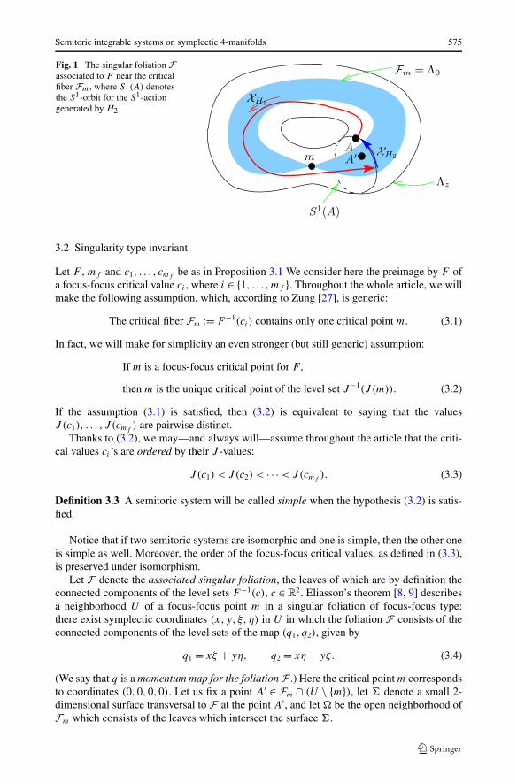
Fig. 1 The singular foliation Fassociated to F near the criticalfiber Fm, where S1(A) denotesthe S1-orbit for the S1-actiongenerated by H2

3.2 Singularity type invariant

Let F , mf and c1, . . . , cmfbe as in Proposition 3.1 We consider here the preimage by F of

a focus-focus critical value ci , where i ∈ {1, . . . ,mf }. Throughout the whole article, we willmake the following assumption, which, according to Zung [27], is generic:

The critical fiber Fm := F−1(ci) contains only one critical point m. (3.1)

In fact, we will make for simplicity an even stronger (but still generic) assumption:

If m is a focus-focus critical point for F,

then m is the unique critical point of the level set J−1(J (m)). (3.2)

If the assumption (3.1) is satisfied, then (3.2) is equivalent to saying that the valuesJ (c1), . . . , J (cmf

) are pairwise distinct.Thanks to (3.2), we may—and always will—assume throughout the article that the criti-

cal values ci ’s are ordered by their J -values:

J (c1) < J (c2) < · · · < J(cmf). (3.3)

Definition 3.3 A semitoric system will be called simple when the hypothesis (3.2) is satis-fied.

Notice that if two semitoric systems are isomorphic and one is simple, then the other oneis simple as well. Moreover, the order of the focus-focus critical values, as defined in (3.3),is preserved under isomorphism.

Let F denote the associated singular foliation, the leaves of which are by definition theconnected components of the level sets F−1(c), c ∈ R

2. Eliasson’s theorem [8, 9] describesa neighborhood U of a focus-focus point m in a singular foliation of focus-focus type:there exist symplectic coordinates (x, y, ξ, η) in U in which the foliation F consists of theconnected components of the level sets of the map (q1, q2), given by

q1 = xξ + yη, q2 = xη − yξ. (3.4)

(We say that q is a momentum map for the foliation F .) Here the critical point m correspondsto coordinates (0,0,0,0). Let us fix a point A′ ∈ Fm ∩ (U \ {m}), let � denote a small 2-dimensional surface transversal to F at the point A′, and let � be the open neighborhood ofFm which consists of the leaves which intersect the surface �.


Since the Liouville foliation in a small neighborhood of � is regular for both momentummaps F and q = (q1, q2), there must be a local diffeomorphism ϕ of R

2 such that q =ϕ ◦ F , and hence we can define a global momentum map = ϕ ◦ F for the foliation, whichagrees with q on U . Write := (H1,H2) and z := −1(z). Note that 0 = Fm. It followsfrom (3.4) that near m the H2-orbits must be periodic of primitive period 2π for any pointin a (non-trivial) trajectory of XH1 .

Suppose that A ∈ z for some regular value z. We define τ1(z), which is a strictly positivenumber, as the time it takes the Hamiltonian flow associated to H1 leaving from A to meetthe Hamiltonian flow associated to H2 which passes through A, and let τ2(z) ∈ R/2πZ bethe time that it takes to go from this intersection point back to A along the Hamiltonian flowline of H2, hence closing the trajectory. Write z = (z1, z2) = z1 + i z2, and let ln z for a fixeddetermination of the logarithmic function on the complex plane. We moreover define thefollowing two functions: {

σ1(z) = τ1(z) + �(ln z),

σ2(z) = τ2(z) − (ln z),(3.5)

where � and respectively stand for the real an imaginary parts of a complex number.In his article [25, Proposition 3.1], Vu Ngo.c proved that σ1 and σ2 extend to smooth andsingle-valued functions in a neighbourhood of 0 and that the differential 1-form

σ := σ1dz1 + σ2dz2 (3.6)

is closed. Notice that if follows from the smoothness of σ2 that one may choose the lift of τ2

to R such that σ2(0) ∈ [0,2π). This is the convention used throughout.

Definition 3.4 [25, Definition 3.1] Let Si be the unique smooth function defined around0 ∈ R

2 such that {dSi = σ,

Si(0) = 0,(3.7)

where σ is the one-form given by (3.6). The Taylor expansion of Si at (0,0) is denotedby (Si)

∞. We say that (Si)∞ is the Taylor series invariant of (M,ω, (J,H)) at the focus-

focus point ci , where i ∈ {1, . . . ,mf }.

The Taylor expansion (S)∞ is a formal power series in two variables with vanishingconstant term.

Lemma 3.5 Let (M1,ω1, (J1,H1)), (M2,ω2, (J2,H2)) be isomorphic 4-dimensional simple

semitoric integrable systems and let ((Sj

i )∞)mi

f

i=1 be the tuple of Taylor series invariants atthe ordered focus-focus critical points of (Mj ,ωj , (Jj ,Hj )), where j ∈ {1,2}. Then the tuple

((S1i )

∞)m1

f

i=1 is equal to the tuple ((S2i )

∞)m2

f

i=1.

This result was proven in [26].

4 Combinatorial invariants of a semitoric system

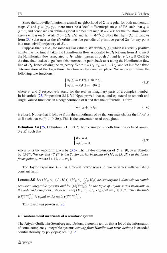
The Atiyah-Guillemin-Sternberg and Delzant theorems tell us that a lot of the informationof some completely integrable systems coming from Hamiltonian torus actions is encodedcombinatorially by polytopes; see Fig. 2.


Fig. 2 Momentum polytope ofCP

2 (left), a Hirzebruch surface(center) and (CP

1)2 (right), allof which determine theisomorphism type of themanifold

Although 4-dimensional semitoric systems are not induced by torus actions, some of theinformation of the system may be combinatorially encoded by a certain equivalence classof rational convex polygons endowed with a collection of vertical weighted lines. This is infact a way of encoding the affine structure induced by the integrable system. Throughoutthis section (M,ω, (J,H)) is a simple 4-dimensional simple semitoric integrable systemwith mf isolated focus-focus singular values, ordered according to (3.3).

4.1 Affine structures

Recall that a map X ⊂ Rm → Y ⊂ R

m is integral-affine on X if it is of the form Aij (·)+ bij ,

where Aij ∈ GL(m,Z) and bij ∈ Rm.

An integral-affine smooth m-dimensional manifold is a smooth m-dimensional manifoldX for which the coordinate changes are integral-affine, i.e. if ϕi : Ui ⊂ R

m → X are thecharts associated to X, for all i, j we have that ϕi ◦ ϕ−1

j , whereever defined, is an integralaffine map. We allow manifolds with boundary and corners, in which case the charts taketheir values in [0,+∞)k × R

m−k for some integer k ∈ {0, . . . ,m}.A map f : X → Y between integral affine manifolds is integral-affine if for each point

x ∈ X there are charts ϕx : Ux → X around x and ψy : Vy → Y around y := f (x) such thatψ−1

y ◦ f ◦ ϕx is integral-affine.As a consequence of the action-angle theorem, any proper Lagrangian fibration

F : M → B naturally defines an integral-affine structure on the base B . This affine structurecan be characterized by the following fact: a local diffeomorphism g : (B,b) → (Rn,0) isintegral-affine if and only if the Hamiltonian flows of the n coordinate functions of g ◦F areperiodic of primitive period equal to 2π . Thus, an integrable system with proper momentummap F = (J,H) defines an integral-affine structure on the set Br of regular values of F . Inour case, this structure will in fact extend to the boundary of Br . Although Br is a subsetof R

2, the integral-affine structure of Br is in general different from the induced canonicalintegral-affine structure of R

2.The integral-affine structure of Br encodes much of the topology of the integrable system

(see [27]) but, as we will see, is far from encoding all its symplectic geometry.

4.2 Generalized toric map

We start with two definitions that we shall need. Let I be the subgroup of the affine groupAff(2,Z) in dimension 2 of those transformations which leave a vertical line invariant, orequivalently, an element of I is a vertical translation composed with a matrix T k , wherek ∈ Z and

T k :=(

1 0k 1

)∈ GL(2,Z). (4.1)

Let � ⊂ R2 be a vertical line in the plane, not necessarily through the origin, which splits it

into two half-spaces, and let n ∈ Z. Fix an origin in �. Let tn� : R2 → R

2 be the identity on


the left half-space, and T n on the right half-space. By definition tn� is piecewise affine. Let�i be a vertical line through the focus-focus value ci = (xi, yi), where 1 ≤ i ≤ mf , and forany tuple �n := (n1, . . . , nmf

) ∈ Zmf we set

t�n := tn1�1

◦ · · · ◦ tnmf

�mf. (4.2)

The map t�n is piecewise affine.In [26, Theorem 3.8] Vu Ngo. c describes how to associate to (M,ω,F = (J,H)) a ra-

tional convex polygon: the image of a certain almost everywhere integral-affine homeomor-phism f : F(M) ⊂ R

2 → � ⊂ R2. Here, B := F(M) is equipped with the natural integral-

affine structure induced by the system, while R2 on the right hand-side is endowed with its

canonical integral-affine structure.Given a sign εi ∈ {−1,+1}, let �

εi

i ⊂ �i be the vertical half line starting at ci at extendingin the direction of εi : upwards if εi = 1, downwards if εi = −1. Let

��ε :=mf⋃i=1

�εi

i .

In this text we shall use the following terminology.

Definition 4.1 A convex polygonal set � is the intersection in R2 of (finitely or infinitely

many) closed half-planes such that on each compact subset of the intersection there is at mosta finite number of corner points. We say that � is rational if each edge is directed along avector with rational coefficients. For brevity, in this paper we usually write “polygon” insteadof “convex polygonal set”.

Notice that such a “convex polygon” is not necessarily compact.

Theorem 4.2 ([26, Theorem 3.8]) For �ε ∈ {−1,+1}mf there is a homeomorphismf = fε : B → R

2 such that

(1) f |(B\��ε ) is a diffeomorphism into its image � := f (B).(2) f |(Br \��ε ) is affine: it sends the integral affine structure of Br to the standard structure

of R2.

(3) f preserves J : i.e. f (x, y) = (x, f (2)(x, y)).(4) For any i ∈ {1, . . . ,mf } and any c ∈ �

εi

i \ {ci} there is an open ball D around c suchthat f |(Br \l�ε ) has a smooth extension on each domain {(x, y) ∈ D |≤ xi} and {(x, y) ∈D | x ≥ xi}. One has the formula:

lim(x,y)→c

x<xi

df (x, y) = T k(c) lim(x,y)→c

x>xi

df (x, y),

where k(c) is the multiplicity of c.(5) The image of f is a rational convex polygon.

Such an f is unique modulo a left composition by a transformation in I.

In order to arrive at the rational convex polygon � in the proof of Theorem 4.2 one cutsthe image (J,H)(M) ⊂ R

2, which is in general not convex, along each of the vertical lines�i , i ∈ {1, . . . ,mf }. One must make a choice of “cut direction” for each vertical line �i , thatis to say that one has to choose whether to cut the set (J,H)(M) along the half-vertical-line �+1

i which starts at ci going upwards, or along the half-vertical-line �−1i which starts at


ci going downwards. Precisely, the definitions of f and � in Theorem 4.2 depend on twochoices in the proof:

(a) an initial set of action variables f0 of the form (J,K) near a regular Liouville torusin [26, Step 2, proof of Theorem 3.8]. If we choose f1 instead of f0 then f has to becomposed on the left by a transformation in I. Naturally, the new polygon is obtainedfrom the initial one by the same transformation;

(b) a tuple �ε of 1 and −1. If we choose �ε ′ instead of �ε we get f ′ = t�u ◦ f (and thus �′ =t�u(�)) with ui = (εi − ε ′

i )/2, by [26, Proposition 4.1, expression (11)].

Definition 4.3 Let (M,ω, (J,H)) be a simple semitoric integrable system and let f achoice of homeomorphism as in Theorem 4.2. We say that:

(i) the map f ◦ (J,H) is a generalized toric momentum map for (M,ω, (J,H));(ii) the rational convex polygon � := f

((J,H)(M)

)is a generalized toric momentum poly-

gon for (M,ω, (J,H)).

For simplicity sometimes we omit the word “generalized” in Definition 4.3.

4.3 Semitoric polygon invariant

Let Polyg(R2) be the space of rational convex polygons in R2. Let Vert(R2) be the set of

vertical lines in R2, i.e.

Vert(R2) = {�λ := {(x, y) ∈ R

2|x = λ}|λ ∈ R}.

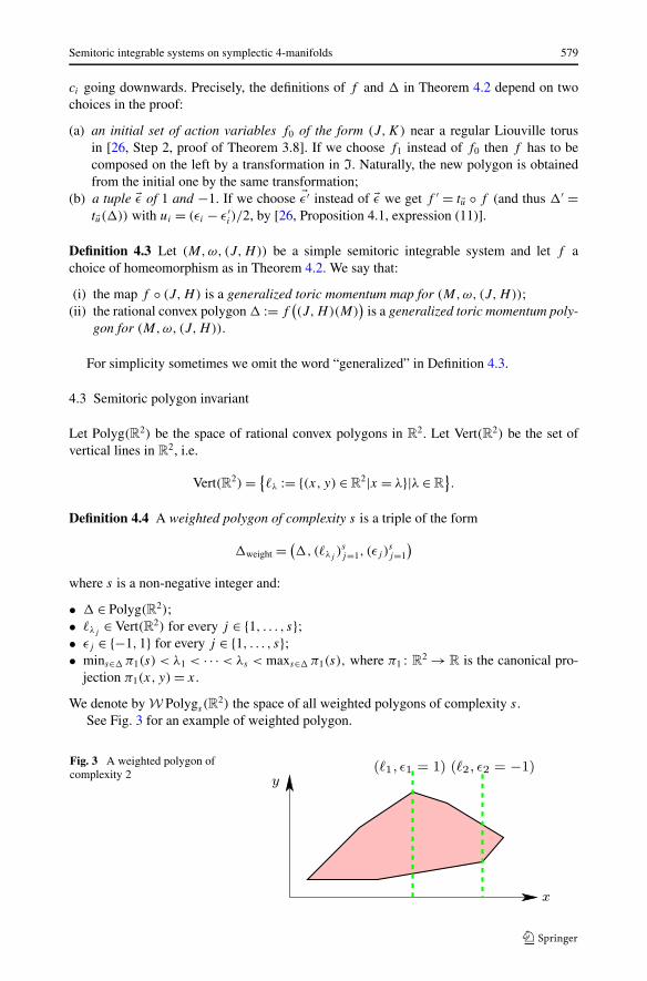
Definition 4.4 A weighted polygon of complexity s is a triple of the form

�weight =(�,(�λj

)sj=1, (εj )

sj=1

)

where s is a non-negative integer and:

• � ∈ Polyg(R2);• �λj

∈ Vert(R2) for every j ∈ {1, . . . , s};• εj ∈ {−1,1} for every j ∈ {1, . . . , s};• mins∈� π1(s) < λ1 < · · · < λs < maxs∈� π1(s), where π1 : R

2 → R is the canonical pro-jection π1(x, y) = x.

We denote by W Polygs(R2) the space of all weighted polygons of complexity s.

See Fig. 3 for an example of weighted polygon.

Fig. 3 A weighted polygon ofcomplexity 2


For any s ∈ N, let

Gs := {−1,+1}s (4.3)

and let

G := {T k|k ∈ Z}, (4.4)

where T is the 2 by 2 matrix (4.1). Consider the action of the product group Gs × G on thespace W Polygs(R

2): the product

((ε ′j )

sj=1, T

k) · (�,(�λj)sj=1, (εj )

sj=1

)

is defined to be

(t�u(T k(�)), (�λj

)sj=1, (ε

′j εj )

sj=1

), (4.5)

where �u = ((εi − ε ′i )/2)s

i=1, and t�u is a map of the form (4.2).

Definition 4.5 Let � be a rational convex polygon obtained from the momentum image(J,H)(M) according to the proof of Theorem 4.2 by cutting along the vertical half-lines�

ε11 , . . . , �

εmfmf

. The semitoric polygon invariant of (M,ω, (J,H)) is the (Gmf× G)-orbit

(Gmf× G) · (�,(�j )

mf

j=1, (εj )mf

j=1

) ∈ W Polygmf(R2)/(Gmf

× G), (4.6)

where W Polygmf(R2) is as in Definition 4.4 and the action of Gmf

× G on W Polygmf(R2)

is given by (4.5).

It follows now from Theorem 4.2 that the semitoric polygon invariant does not dependon the isomorphism class of the system.

Lemma 4.6 Let (M1,ω1, (J1,H1)), (M2,ω2, (J2,H2)) be isomorphic 4-dimensional semi-toric integrable systems. Then the semitoric polygon invariant of (M1,ω1, (J1,H1)) is equalto the semitoric polygon invariant of (M2,ω2, (J2,H2)).

5 Geometric invariants of a semitoric system

The invariants we have described so far are not enough to determine whether two4-dimensional semitoric systems are isomorphic. In this section we introduce two globalgeometric invariants, which encode a mixture of information about local and global behav-ior. Throughout, (M,ω, (J,H)) is a 4-dimensional semitoric integrable system with mf

isolated focus-focus singular values.

5.1 The volume invariant

The invariant we introduce next is easy to define using the combinatorial ingredients wehave by now introduced. Consider a focus-focus critical point mi whose image by (J,H) isci for i ∈ {1, . . . ,mf }, and let � be a rational convex polygon corresponding to the system(M,ω, (J,H)), cf. Definition 4.5.


Lemma 5.1 If μ is a toric momentum map for the simple semitoric system (M,ω, (J,H))

corresponding to �, cf. Definition 4.3, then the image μ(mi), where i ∈ {1, . . . ,mf }, is apoint lying in the interior of the polygon �, along the line �i . The vertical distance

hi := μ(mi) − mins∈�i∩�

π2(s) > 0 (5.1)

between μ(mi) and the point of intersection of �i with the image polytope with lowesty-coordinate, is independent of the choice of momentum map μ. Here π2 : R

2 → R is thecanonical projection π2(x, y) = y.

Lemma 5.1 follows from the fact that two different toric momentum maps only differ bypiecewise affine transformations, which all act on any fixed vertical line as translations.

Definition 5.2 We say that the vertical distance (5.1) between μ(mi) and the point of inter-section of �i with the image polytope that has the lowest y-coordinate is the height of thefocus-focus critical value ci , where i ∈ {1, . . . ,mf }.

Remark 5.1 One can give a geometrical meaning to the height of the focus-focus criticalvalues. Let Yi = J−1(ci). This singular manifold splits into two parts, Y +

i and Y −i defined

as Yi ∩ {H > H(mi)} and Yi ∩ {H < H(mi)}, respectively. The height of the focus-focuscritical value ci is simply the Liouville volume of Y −

i .

Since isomorphic systems share the same set of momentum polygons, we have the fol-lowing result.

Lemma 5.3 Let (M1,ω1, (J1,H1)), (M2,ω2, (J2,H2)) be isomorphic simple 4-dimensional

semitoric integrable systems and let (hj

i )mi

f

i=1 be the tuple of heights of focus-focus critical

values of (Mj ,ωj , (Jj ,Hj )), j ∈ {1,2}. Then the tuple (h1i )

m1f

i=1 is equal to the tuple (h2i )

m2f

i=1.

The volume invariant is very easy to compute from a weighted polygon, and hence it is aquick way to rule out that two semitoric integrable systems are not isomorphic.

5.2 The twisting-index invariant

For clarity, we divide the construction of the twisting index invariant into five steps. Let

�weight :=(�,(�j )

mf

j=1, (εj )mf

j=1

) ∈ W Polygmf(R2), (5.2)

be a weighted polygon as in expression (4.6), representing the orbit given by the semitoricpolygon invariant of the system (M,ω, (J,H)), cf. Definition 4.5, where recall that thepolygon � is obtained from the momentum image (J,H)(M) according to the proof ofTheorem 4.2 by cutting along the vertical lines �1, . . . , �mf

in the direction of ε1, . . . , εmf,

i.e. upwards if εi is +1 and downwards otherwise. Write F = (J,H), c1, . . . , cmffor the

focus-focus critical values.In the first three steps we define for each i ∈ {1, . . . ,mf }, an integer ki that we shall

call the twisting index of the focus-focus value ci , on which we built to construct the actualinvariant associated to (M,ω, (J,H)) in Step 5.


Step 1: an application of Eliasson’s theorem. Let (e1, e2) be the canonical basis of R2. Let

� = �+1i ⊂ R

2 be the vertical half-line starting at ci and pointing in the direction of εie2.Let us apply Eliasson’s theorem in a small neighbourhood W = Wi of the focus-focus

critical point mi = F−1(ci): there exists a local symplectomorphism φ : (R4,0) → W , anda local diffeomorphism g of (R2,0) such that

F ◦ φ = g ◦ q, (5.3)

where q is the quadratic momentum map given by (3.4). Since the second component,q2 ◦ φ−1, has a 2π -periodic Hamiltonian flow, it must be equal to J in W , up to a sign.Composing if necessary φ by the canonical transformation (x, ξ) �→ (−x,−ξ), one canalways assume that q2 = J ◦ φ in W . This means that g is of the form

g(q1, q2) = (q2, g2(q1, q2)). (5.4)

Moreover, upon composing φ by the canonical transformation (x, y, ξ, η) �→(−ξ,−η,x, y), which changes (q1, q2) into (−q1, q2), one can always assume that

∂g2

∂q1(0) > 0. (5.5)

In particular, near the origin � is transformed by g−1 into the positive real axis if εi = 1, orthe negative real axis if εi = −1.

Step 2: the smooth vector field Xp . Let us now fix the origin of angular polar coordinates inR

2 on the positive real axis. Let V = F(W) and define F = (H1,H2) = g−1 ◦ F on F−1(V )

(notice that H2 = J ). Now recall from Sect. 3.2 that near any regular torus there exists aHamiltonian vector field Xp , whose flow is 2π -periodic, defined by

2π Xp = (τ1 ◦ F )XH1 + (τ2 ◦ F )XJ , (5.6)

where τ1 and τ2 are functions on R2 \ {0} satisfying (3.5), with σ1(0) > 0. In fact τ2 is

multivalued, but we determine it completely in polar coordinates with angle in [0,2π) byrequiring continuity in the angle variable and σ2(0) ∈ [0,2π). In case εi = 1, this defines Xp

as a smooth vector field on F−1(V \ �). In case εi = −1 we keep the same τ2-value on thenegative real axis, but extend it by continuity in the angular interval [π,3π). In this way Xp

is again a smooth vector field on F−1(V \ �).

Step 3: twisting index of a weighted polygon at a focus-focus singularity. Let μ be thegeneralized toric momentum map, cf. Definition 4.3, associated to the polygon �. OnF −1(V \ �), μ is smooth, and its components (μ1,μ2) = (J,μ2) are smooth Hamiltoni-ans, whose vector fields (XJ , Xμ2) are tangent to the foliation, have a 2π -periodic flow, andare a.e. independent. Since the couple (XJ , Xp) shares the same properties, there must bea matrix A ∈ GL(2,Z) such that (XJ , Xμ2) = A(XJ , Xp). This is equivalent to saying thatthere exists an integer ki ∈ Z such that

Xμ2 = ki XJ + Xp. (5.7)

Proposition 5.4 For a fixed weighted polygon �weight as in (5.2), the integer ki in (5.7) iswell defined for each i ∈ {1, . . . ,mf }, i.e. it does not depend on


(a) the choice of the periodic Hamiltonian Xp ;(b) the transformations involved in Eliasson’s normal form (5.3), with the sign con-

straints (5.4) and (5.5).

Proof It follows from [25, Lemma 4.1] that changing the transformations involved in Elias-son’s normal form [8, 9] can only modify g2—and hence H1—by a flat term. Suppose X ′

p isanother admissible choice for a Hamiltonian of the form

2π X ′p = (τ ′

1 ◦ F ′)XH ′1+ (τ ′

2 ◦ F ′)XJ .

Since X ′p has a 2π -periodic flow, there must be coprime integers a, b in Z such that

X ′p = aXp + bXJ . (5.8)

Inserting (5.6), we see that there exist functions Z1 and Z2 that vanish at all orders at theorigin such that

2π X ′p = (aτ1 ◦ F + Z1)XH ′

1+ (aτ2 ◦ F + 2πb + Z2)XJ .

From this we see that, up to a flat function, τ ′1 = aτ1 and τ ′

2 = aτ2 + 2πb. Because ofthe logarithmic asymptotics required in (3.5), the first equation requires a = 1. But then, thesecond equation with the restriction that both σ2(0) and σ ′

2(0) must be in [0,2π) implies thatb = 0. Recalling (5.8) we obtain X ′

p = Xp , which shows that ki is indeed well-defined. �

Definition 5.5 Let �weight be a fixed weighted polygon as in (5.2). For each i ∈ {1, . . . ,mf },the integer ki defined in (5.7) is called the twisting index of �weight at the focus-focus criticalvalue ci .

The integer ki in Definition 5.5 is still not the relevant object that we intend to associateto the semitoric system, but we shall build on its definition to construct the actual invariant.

Step 4: the privileged momentum map. We explain how there is a reasonable way to“choose” a momentum map for (M,ω, (J,H)).

Lemma 5.6 There exists a unique smooth function Hp on F−1(V \ �) the Hamiltonianvector field of which is Xp and such that limm→mi

Hp = 0.

Proof Near a regular torus Xp is a Hamiltonian vector field of a function of the formf (H1, J ), and by construction ∂if = τi/2π, i ∈ {1,2}. Therefore, using (3.5) we can checkthat 2πf (z) = S(c) − �(z ln z − z) + Const, where S is smooth at the origin, which showsthat f has a limit as z ∈ R

2 \ ([0,∞) × {0}) tends to the origin. In fact, f has a continuousextension to R

2, entailing that Hp extends to a continuous function on F−1(V ). �

Definition 5.7 Let (M,ω, (J,H)) be a 4-dimensional simple semitoric integrable system,and let Hp be the unique smooth function defined in Lemma 5.6. We say that the toricmomentum map ν := (J,Hp) is the privileged momentum map for (J,H) around the focus-focus value ci , for each i ∈ {1, . . . ,mf }.

The map ν in Definition 5.7 depends on the cut �, that is to say, on the sign εi . Moreover,we have the following.


(a) If ki is the twisting index of ci , one has

μ = T ki ν on F−1(V ). (5.9)

(b) If we transform the polygon � by a global affine transformation in T r ∈ I this has noeffect on the privileged momentum map ν, whereas it changes μ into T rμ.

From the characterization (5.9), it follows that all the twisting indices ki are replaced byki + r .

With this preparation we are now ready to define the twisting index invariant.

Step 5: the twisting index invariant. We give the definition of the twisting index invariantas an equivalence class of weighted polygons labelled by a collection of integers.

Proposition 5.8 If two weighted polygons �weight and �′weight lie in the same Gmf

-orbit,for the Gmf

-action induced by (4.5), then the twisting indexes ki, k′i associated to �weight

and �′weight at their respective focus-focus critical values ci, c

′i are equal, for each i ∈

{1, . . . ,mf }.

Proof For εi = ±1, we denote by μ± and ν±, as in (5.9) above, the generalized toric mo-mentum map and the privileged momentum map, cf. Definition 5.7 at ci .

With the notations of Sect. 4, we have

μ− = t�iμ+.

On the other hand, from the definition of τ2 in each case, we see that Xp,− = Xp,+ on theleft-hand side of � (that is to say, J < 0), while

Xp,− = Xp,+ + 2π XJ

on the right hand side (J > 0). This means that ν− = t�iν+. From the characterization of the

twisting index by (5.9), using that t�icommutes with T , we see that ki,+ = ki,−. �

Recall the groups Gs and G given by (4.3) and (4.4) respectively, and the action of Gs × Gon W Polygs(R

2), cf. Definition 4.5. Consider the action of the product group Gs × G on thespace W Polygs(R

2) × Zms : the product

((ε ′j )

sj=1, T

k) �(�,(�λj

)sj=1, (εj )

sj=1, (ki)

si=1

)is defined to be

(t�u(T k(�)), (�λj

)sj=1, (ε

′j εj )

sj=1, (ki + k)s

i=1

). (5.10)

where �u = (εi − ε ′i )/2)s

i=1. Here T is the 2 by 2 matrix (4.1) and t�u is of the form (4.2).

Definition 5.9 The twisting-index invariant of (M,ω, (J,H)) is the (Gmf× G)-orbit of

weighted polygon labelled by twisting indexes at the focus-focus singularities of the systemgiven by

(Gmf× G) �

(�,(�j )

mf

j=1, (εj )mf

j=1, (ki)mf

i=1

) ∈ (W Polygmf(R2) × Z

mf )/(Gmf× G), (5.11)

where W Polygmf(R2) is defined in Definition 4.4 and the action of Gmf

× G on

W Polygmf(R2) × Z

mf is given by (5.10).


Here again, our definition is invariant under isomorphism.

Lemma 5.10 Let (M1,ω1, (J1,H1)), (M2,ω2, (J2,H2)) be isomorphic 4-dimensional sim-ple semitoric integrable systems. Then their corresponding twisting-index invariants areequal.

Remark 5.2 We would like to emphasize again that the twisting index is not a semiglobalinvariant of the singular fibration in a neighbourhood of the focus-focus fibre. Such semi-global fibrations are completely classified in [25], and the twisting index does not play anyrole there. It is instead a global invariant characterizing the way the fibers near a particularfocus-focus point stand with respect to the rest of the fibration.

6 Main theorem: statement

We consider a simple semitoric system and assign to it a list of invariants as above. Thegeneral idea is simple: the complete invariant is just a rational convex polygon having afinite number of distinguished interior points (the focus-focus critical values), each of thembeing decorated by a Taylor series and an integer (the twisting index).

The technical difficulty is that the polygon is in fact not unique. One could remove part ofthe trouble by fixing all the signs εi in Theorem 4.2 to be positive, but this would hide a keyfeature (and motivation); indeed, switching from one polygon to another is what is expectedto happen during a generic bifurcation of semitoric systems (see [26]). Thus we do no wantto fix the signs, and instead deal with equivalence classes. Then the vertical positions of thefocus-focus critical values may change, and only their heights (with respect to the bottomline of the polygon) are well defined. What’s more, the twisting indices themselves arerelevant only modulo the addition of a common integer.

After these considerations, the list of invariants we propose is the following. Recall thatthe focus-focus points are ordered according to (3.3).

Definition 6.1 Let (M,ω, (J,H)) be a 4-dimensional simple semitoric integrable system.The list of invariants of (M,ω, (J,H)) consists of the following items.

(i) The integer number 0 ≤ mf < ∞ of focus-focus singular points, see Sect. 3.1.(ii) The mf -tuple ((Si)

∞)mf

i=1, where (Si)∞ is the Taylor series of the ith focus-focus point,

see Sect. 3.2.(iii) The semitoric polygon invariant: the (Gmf

× G)-orbit

(Gmf× G) · �weight ∈ W Polyg(R2)/(Gmf

× G)

of the weighted polygon �weight := (�, (�j )mf

j=1, (εj )mf

j=1), cf. Definition 4.5.

(iv) The mf -tuple of positive real numbers (hi)mf

i=1, where hi is the height of the ith focus-focus point, see Sect. 5.1.

(v) The twisting-index invariant: the (Gmf× G)-orbit

(Gmf× G) �

(�weight, (ki)

mf

i=1

) ∈ (W Polyg(R2) × Zmf )/(Gmf

× G)

of the weighted polygon labelled by the twisting-indexes (�weight, (ki)mf

i=1), cf. Defini-tion 5.9.


In the above list invariant (v) determines invariant (iii), so we could have ignored thelatter. We have kept this list as it appears naturally in the construction of the invariants.Indeed the definition of invariant (iii) is needed to construct invariant (v). One may alsoargue that it is worthwhile for practical purposes to list (iii), as it is easier to compute than(v) and hence if two systems do not have the same invariant (iii) we know they are notisomorphic without having to compute (v). Notice that all these invariants are based uponthe standard affine plane R

2, which makes them relatively easy to visualize, even when theireffect on the system (M,ω, (J,H)) may be delicate to understand.

Recall that if (M1,ω1, (J1,H1)) and (M2,ω2, (J2,H2)) are 4-dimensional semitoric in-tegrable systems, we say that they are isomorphic if there exists a symplectomorphism

ϕ : M1 → M2, such that ϕ∗(J2,H2) = (J1, f (J1,H1))

for some smooth function f such that ∂f

∂H1never vanishes. Our main theorem is the follow-

ing.

Theorem 6.2 Two 4-dimensional simple semitoric integrable systems (M1,ω1, (J1,H1))

and (M2,ω2, (J2,H2)) are isomorphic if and only if the list of invariants (i)–(v), as in Defin-ition 6.1, of (M1,ω1, (J1,H1)) is equal to the list of invariants (i)–(v) of (M2,ω2, (J2,H2)).

The proof of Theorem 6.2 is sufficiently involved that is better organized in an indepen-dent section. In the proof we use notable results of several authors, in particular Eliasson,Duistermaat, Dufour-Molino, Liouville-Mineur-Arnold and Vu Ngo. c. We combine theseresults with new ideas to construct explicitly an isomorphism between two semitoric in-tegrable systems that have the same invariants, in the spirit of Delzant’s proof [3] for thecase when the system defines a Hamiltonian 2-torus action. Because in our context we havefocus-focus singularities a number of delicate problems arise that one has to deal with toconstruct such an isomorphism. As a matter of fact, it is remarkable how the behavior of thesystem near a particular singularity has a subtle global effect on the system.

Remark 6.1 When the system is in fact toric, then there is no focus-focus point, and thewhole list of invariants breaks down to a mere rational convex polygon defined modulo I.This is of course the usual Delzant polygon; the action of I reflects the fact that the definitionof isomorphism is less strict that in Delzant’s situation.

Example 6.3 The simplest non-toric, non-compact example is probably the “coupled spin-oscillator” model described in [26, Sect. 6.2]. In this case M = S2 ×R

2, where S2 is viewedas the unit sphere in R

3 with coordinates (x, y, z), and the second factor R2 is equipped with

coordinates (u, v). We define

J := (u2 + v2)/2 + z and H := 1

2(ux + vy).

For the standard product symplectic structure on M , the system (J,H) is a simple semitoricsystem, with one single focus-focus point at ((0,0,1), (0,0)) ∈ S2 ×R

2, and hence mf = 1.The image of the momentum map (J,H) is depicted in Fig. 4.

Because there is only one focus-focus point, the twisting-index invariant contains noinformation. One can take for instance k1 = 0.

The remaining list of invariants is depicted in Fig. 4, except for the Taylor series invariant(S1) which, even in this simple example, is difficult to compute explicitly; in rather special


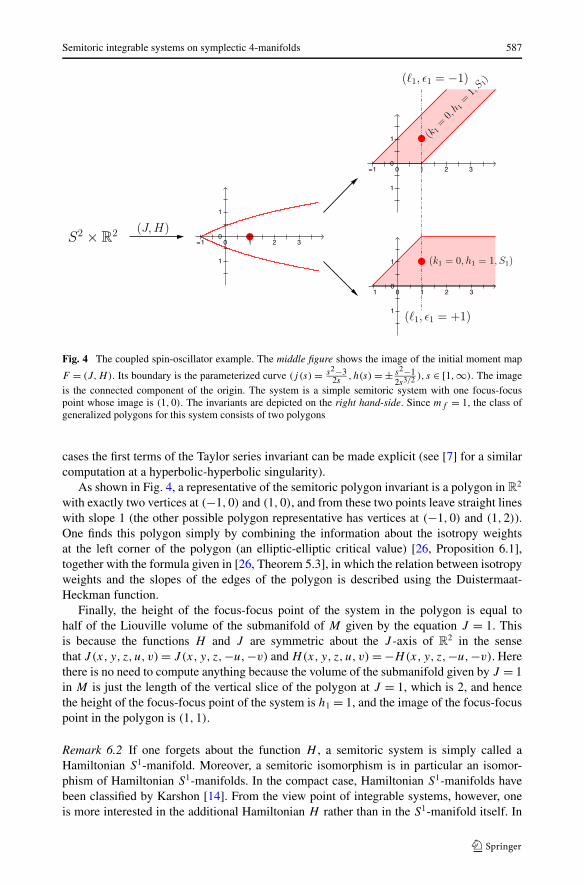
Fig. 4 The coupled spin-oscillator example. The middle figure shows the image of the initial moment map

F = (J,H). Its boundary is the parameterized curve (j (s) = s2−32s

, h(s) = ± s2−12s3/2 ), s ∈ [1,∞). The image

is the connected component of the origin. The system is a simple semitoric system with one focus-focuspoint whose image is (1,0). The invariants are depicted on the right hand-side. Since mf = 1, the class ofgeneralized polygons for this system consists of two polygons

cases the first terms of the Taylor series invariant can be made explicit (see [7] for a similarcomputation at a hyperbolic-hyperbolic singularity).

As shown in Fig. 4, a representative of the semitoric polygon invariant is a polygon in R2

with exactly two vertices at (−1,0) and (1,0), and from these two points leave straight lineswith slope 1 (the other possible polygon representative has vertices at (−1,0) and (1,2)).One finds this polygon simply by combining the information about the isotropy weightsat the left corner of the polygon (an elliptic-elliptic critical value) [26, Proposition 6.1],together with the formula given in [26, Theorem 5.3], in which the relation between isotropyweights and the slopes of the edges of the polygon is described using the Duistermaat-Heckman function.

Finally, the height of the focus-focus point of the system in the polygon is equal tohalf of the Liouville volume of the submanifold of M given by the equation J = 1. Thisis because the functions H and J are symmetric about the J -axis of R

2 in the sensethat J (x, y, z,u, v) = J (x, y, z,−u,−v) and H(x,y, z,u, v) = −H(x,y, z,−u,−v). Herethere is no need to compute anything because the volume of the submanifold given by J = 1in M is just the length of the vertical slice of the polygon at J = 1, which is 2, and hencethe height of the focus-focus point of the system is h1 = 1, and the image of the focus-focuspoint in the polygon is (1,1).

Remark 6.2 If one forgets about the function H , a semitoric system is simply called aHamiltonian S1-manifold. Moreover, a semitoric isomorphism is in particular an isomor-phism of Hamiltonian S1-manifolds. In the compact case, Hamiltonian S1-manifolds havebeen classified by Karshon [14]. From the view point of integrable systems, however, oneis more interested in the additional Hamiltonian H rather than in the S1-manifold itself. In


fact, using Karshon’s classification would imply losing track of one of integrable systems’arguably most important structure, the integral affine structure of the image of F . This iswhy Karshon’s results are not used in this article. It would be nevertheless interesting tounderstand how the labelled graphs she uses can be obtained from our labelled polygons. Inthis process, obviously, we expect to lose much of the information about focus-focus singu-larities. For instance, the same simple Hamiltonian S1 action on S2 × S2 can be either toricor truly semitoric, as in the example above.

7 Proof of main theorem

The left-to-right implication follows from putting together Lemmas 3.2, 3.5, 4.6, 5.3and 5.10. The proof of the right-to-left implication breaks into three steps. Let F1 = (J1,H1)

and let F2 = (J2,H2).

• First, we reduce to a case where the images F1(M1) and F2(M2) are equal.• Second, we prove that this common image can be covered by open sets �α , above each

of which F1 and F2 are symplectically interwined.• The last step is to glue together these local symplectomorphisms, in this way constructing

a global symplectomorphism φ : M1 → M2 such that F1 = F2 ◦ φ.

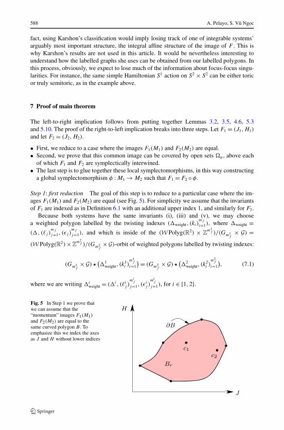
Step 1: first reduction The goal of this step is to reduce to a particular case where the im-ages F1(M1) and F2(M2) are equal (see Fig. 5). For simplicity we assume that the invariantsof F1 are indexed as in Definition 6.1 with an additional upper index 1, and similarly for F2.

Because both systems have the same invariants (i), (iii) and (v), we may choosea weighted polygon labelled by the twisting indexes (�weight, (ki)

mf

i=1), where �weight =(�, (�j )

mf

j=1, (εj )mf

j=1), and which is inside of the (W Polyg(R2) × Zm1

f )/(Gm1f

× G) =(W Polyg(R2) × Z

m2f )/(Gm2

f× G)-orbit of weighted polygons labelled by twisting indexes:

(Gm1f

× G) �(�1

weight, (k1i )

m1f

i=1

) = (Gm2f

× G) �(�2

weight, (k2i )

m2f

i=1

), (7.1)

where we are writing �iweight = (�i, (�i

j )mi

f

j=1, (εij )

mif

j=1), for i ∈ {1,2}.

Fig. 5 In Step 1 we prove thatwe can assume that the“momentum” images F1(M1)

and F2(M2) are equal to thesame curved polygon B . Toemphasize this we index the axesas J and H without lower indices


Let μ1,μ2 respectively be associated toric momentum maps to F1 and F2 for the polygon� in Theorem 4.2 and Definition 4.3. There are homeomorphisms g1, g2 : � → � such that

F1 = g1 ◦ μ1, F2 = g2 ◦ μ2.

Consider the map h := g1 ◦ g−12 . We wish to replace F2 by F2 = h ◦ F2. Then, obviously,

Image(F2) = g1(�) = Image(F1).

In order for F2 to define a semi-toric completely integrable system isomorphic to F2, weneed to prove that h(x, y) = (x, f (x, y)) for some smooth function f . In fact, it followsfrom Theorem 4.2 that h has this form, but for some f which is a priori not smooth. Thecrucial point here is to show that, because F1 and F2 have the same invariants, h is in factsmooth.

Claim 7.1 The map h extends to an S1-equivariant diffeomorphism of a neighborhood ofF2(M2) into a neighborhood of F1(M1).

The map h is a already a homeomorphism. We need to show that it is a local diffeomorphismeverywhere. Let us denote by c

j

i for j ∈ {1,2} and i ∈ {1, . . . ,mf } the focus-focus criticalvalues of Fj . Again we let (e1, e2) be the canonical basis of R

2 and let �j

i ⊂ R2 be the

vertical half-line starting at cj

i and pointing in the direction of εj e2.Since the tuple of heights of the focus-focus points given by invariant (iv) are the same

for both systems, g−11 (c1

j ) = g−12 (c2

j ) and g−11 (�1

i ) = g−12 (�2

i ). Hence h is smooth away fromthe union of all �2

i , i ∈ {1, . . . ,mf }.Let us now fix some i ∈ {1, . . . ,mf } and let Uz be a small ball around a point z ∈ �2

i \{c2i }.

For simplifying notations, we shall drop the various subscripts i. Recall that Uz inherits fromF2(M2) an integral-affine structure. Let ϕz : Uz → Uz be an oriented affine chart, with Uz aneighborhood of the origin in R

2, sending the vertical axis to �2. In order to show that h issmooth on Uz, we consider the two halves of the ball Uz:

U+z = Uz ∩ {x ≥ xc} and U−

z = Uz ∩ {x ≤ xc},where xc is the abscissa of c2. Of course, the restrictions of ϕz to each half Uz ∩ {x ≥ 0}and Uz ∩ {x ≤ 0} are admissible affine charts for U+

z and U−z , respectively. Let us call these

restrictions ϕ±z . Let y = h(z), Vy = h(Uz) and V ±

y = h(U±z ). Using the natural integral-

affine structure on F1(M1), we can similarly introduce an affine chart ψy for Vy and thecorresponding restrictions ψ±

y . We are now going to use the following facts:

1. On each half U+z and U−

z , h is an integral-affine isomorphism: U±z → V ±

y .2. The differential dh is continuous on U .

The first fact implies, by definition, that the map

ν± := (ψ±y )−1 ◦ h ◦ ϕ±

z ,

wherever defined, is of the form A±(·) + b±, for some matrix A± ∈ GL(2,Z) and someconstant b± ∈ R

2. Evaluating the differentials at the origin, we immediately deduce from thesecond fact that A+ = A−. So, ν± should be just a translation. But h itself being continuouson the line segment �2, we must have b+ = b−. It follows that, on Uz, h is equal to ψy ◦ L ◦


ϕ−1z , where L is the affine transformation A+(·) + b+ = A−(·) + b−. So h is indeed smooth

on Uz.We have left to show that h is smooth at a focus-focus critical value c2. The fact

that we are assuming that invariant (ii) is the same for both systems means that the cor-responding symplectic invariants power series (S)∞ are the same for both systems im-plies, by the semi-global result of Vu Ngo.c [25, Theorem 2.1], that there exist a neigh-borhood V (c1) of c1, a neighborhood V (c2) of c2, a semi-global symplectomorphismϕ : F−1

1 (V (c1))) → F−12 (V (c2)) and a local diffeomorphism g : V (c2) → V (c1) such that

F1 = g ◦ F2 ◦ ϕ. Now, from Lemma 5.6 we know that there exists a privileged toric mo-mentum map, cf. Definition 5.7, for each system above the domain V (cj ) \ �j , j ∈ {1,2},cf. Definition 5.7. We denote by ν1 this momentum map for the system induced by F1, andν2 for the system induced by F2. Since ν1 and ν2 are semi-global symplectic invariants, onehas ν1 = ν2 ◦ ϕ.

By (7.1) the focus-focus critical values c1 of the semitoric systems F1 and c2 of F2 havethe same twisting-index invariant k with respect to the common polygon �. In view of thecharacterization of expression (5.9), we get

μ1 = T kν1 and μ2 = T kν2, (7.2)

and therefore

μ1 = μ2 ◦ ϕ.

Thus we can write g−11 F1 = g−1

2 F2 ◦ ϕ, or

F1 = h ◦ g−1 ◦ F1.

Using that F1 is a submersion on a neighborhood of any regular torus, and the fact thath ◦ g−1 is smooth at the corresponding regular values of F1, we get that

h ◦ g−1 = Id on V (c1). (7.3)

By continuity, this also holds at c1. Hence h = g is smooth at c2, which proves the claim.

Step 2: Local symplectomorphisms From step 1 we can assume that

F1 = g1 ◦ μ1, F2 = g1 ◦ μ2 (7.4)

and hence F1(M1) = F2(M2). In this second step we prove that this common image can becovered by open sets �α , above each of which F1 and F2 are symplectically interwined.

Claim 7.2 There exists a locally finite open cover (�α)α∈A of F1(M1) = F2(M2) such that

1. all �α , α ∈ A are simply connected, and all intersections are simply connected;2. for each α ∈ A, �α contains at most one critical value of rank 0 of Fi , for any i ∈ {1,2};3. for each α ∈ A, there exists a symplectomorphism ϕα : F−1

1 (�α) → F−12 (�α) such that

F1 = F2 ◦ ϕα on F−11 (�α).

We prove this claim next. Recall that the toric momentum maps μ1 and μ2 have byhypothesis the same image, which is the polygon �. We can define an open cover �α of �

with open balls, satisfying points (1) and (2). When the ball �α contains critical value of


rank 0, we may assume that this critical value is located at its center. Similarly, when a ballcontains critical values of rank 1, we may assume that the set of rank 1 critical values in thisball is a diameter. Then we just define

�α = g1(�α).

Notice that in doing so we ensure that the number and type of critical values of Fi in �α arethe same for i = 1 and i = 2. For proving point (3) we distinguish four cases:

(a) �i,α contains no critical point of Fi ;(b) �i,α contains critical points of rank 1, but not of rank 0;(c) �i,α contains a rank 0 critical point, of elliptic-elliptic type;(d) �i,α contains a rank 0 critical point, of focus-focus type.

The reasoning for all cases follows the same lines, but we keep these cases separated for thesake of clarity.

Case (a) Let us fix a point cα ∈ �α . By Liouville-Mineur-Arnold theorem [5], applied foreach momentum map Fi over the simply connected open set �α , there exists a symplecto-morphism ϕi,α : F−1

i (�α) → T∗T

2 and a local diffeomorphism hi : (R2,0) → (R2, cα) suchthat

Fi = hi(ξ1, ξ2) ◦ ϕi,α.

Here we use the notation (x1, x2, ξ1, ξ2) for canonical coordinates in T∗T

2, where the zerosection is given by {ξ1 = ξ2 = 0}.

In fact because of (7.4), μi = g−11 hi(ξ1, ξ2) ◦ ϕi,α . Since both μi and (ξ1, ξ2) are toric

momentum map, this implies that g−11 hi is an affine map with a linear part Bi ∈ GL(2,Z).

Now we can define a linear symplectomorphism in a block-diagonal way

Si =(

tBi 00 B−1

i .

)

Obviously (ξ1, ξ2) ◦ Si = B−1i ◦ (ξ1, ξ2). From now on we replace ϕi,α by Si ◦ ϕi,α , which

reduces us to the case Bi = Id.Now, let ϕα := ϕ−1

2,α ◦ ϕ1,α . We have the relation

F1 = (h1h−12 ) ◦ F2 ◦ ϕ−1

2,α ◦ ϕ1,α = g1(g−11 h1)(g

−11 h2)

−1g−11 ◦ ϕα.

The affine diffeomorphism (g−11 h1)(g

−11 h2)

−1 is tangent to the identity and fixes the point cα ;hence it is the identity, and we obtain, as required:

F1 = F2 ◦ ϕα, on F−11 (�α).

Case (b) Above �α , the momentum map has singularities, so we cannot apply the action-angle theorem. However, there is still a T

2-action, and it is well known that an “action-anglewith elliptic singularities” theorem holds (see [4] or [20]). Precisely, we fix a point cα ∈ �α

that is a critical value of F1 and F2, and then for each i ∈ {1,2}, there exists a symplectomor-phism ϕi,α : F−1

i (�α) → T∗R × T∗

T1 and a local, orientation preserving diffeomorphism

hi : (R2,0) → (R2, cα) such that

Fi = hi(q1, ξ2) ◦ ϕi,α.


Here T∗R has canonical coordinates (x1, ξ1), q1 = (x2

1 + ξ 21 )/2, and T∗

T1 has canonical

coordinates (x2, ξ2). As before, one has

μi = g−11 hi(q1, ξ2) ◦ ϕi,α,

and g−11 hi is an affine map with a linear part in SL(2,Z).

Since hi must preserve the set of critical values, it must send the vertical axis“q1 = 0” ⊂ R

2 to the set of critical values in �α . Hence g−11 hi sends the vertical axis to

the corresponding diameter in �α . Moreover, since by hypothesis the images of μ1 and μ2

are the same, the set “q1 > 0” corresponds via g−11 h1 and g−1

1 h2 to the same half of theball �α . In other words, the vector e2 = (0,1) is an eigenvector for the linear part B of(g−1

1 h1)−1g−1

1 h2, with eigenvalue 1.Therefore, B is of the form

( 1 0k 1

), for some integer k ∈ Z. Now, consider the map

S(x1, x2, ξ1, ξ2) = (x ′1, x

′2, ξ

′1, ξ

′2) given by

⎧⎪⎪⎨⎪⎪⎩

(x ′1 + iξ ′

1) = eikx2(x1 + iξ1),

x ′2 = x2,

ξ ′2 = ξ2 + kq1.

(7.5)

In complex coordinates,

dξ1 ∧ dx1 = 1

2idz1 ∧ dz1,

so it is easy to check that S is symplectic. Moreover,

(q1, ξ2) ◦ S =(

1 0k 1

)(q1, ξ2) = B(q1, ξ2).

We can write

F1 = h1B−1(q1, ξ2) ◦ S ◦ ϕ1,α,

and hence, letting ϕα := ϕ−12,α ◦ S ◦ ϕα ,

F1 = (h1B−1h−1

2 ) ◦ F2 ◦ ϕα.

Consider the affine map (g−11 h1)

−1g−11 h2B

−1. Its linear part is the identity, and it fixedthe origin; thus it is the identity. This implies that h1B

−1h−12 = Id.

Case (c) Using Eliasson’s local normal form for elliptic-elliptic singularities [8, 9], wehave the existence of a symplectomorphism ϕα and a local diffeomorphism h such that

F1 = h ◦ F2 ◦ ϕα.

Again, because of (7.4), μ2 = g−11 hg1 ◦μ1 ◦ ϕα , and g−1

1 hg1 ∈ GL(2,Z). But since the imageof μ1 and the image of μ2 are the same, then g−1

1 hg1 must send the corner of the polygon toitself. Since it is a Delzant corner, g−1

1 hg1 must be the identity.


Case (d) From (7.4), the momentum maps F1 and F2 have the same focus-focus criticalvalues c1, . . . , cmf

. We wish here to interwine both systems above a small neighborhood ofeach ci . In order to ease notations, let us drop the subscript i, as the construction can berepeated for each focus-focus point.

The behaviour of the system in a neighborhood of c is given by Vu Ngo.c’s theorem,which we already used for the proof of Claim 7.1. Precisely [26, Theorem 2.1] gives theexistence of a neighborhood V (c) of c together with an equivariant symplectomorphism

ψ : F −11 (V (c)) → F−1

2 (V (c)) (7.6)

and a diffeomorphism g such that

F1 = g ◦ F2 ◦ ψ. (7.7)

Now, we may argue exactly as in (7.2)–(7.3), keeping in mind that we are now in the casewhere h = Id. Hence g also must be the identity map.

This concludes the proof of Claim 7.2 and hence Step 2.

Step 3: local to global In this last step is to glue together the local symplectomorphisms ofStep 2, thus constructing a global symplectomorphism φ : M1 → M2 such that F1 = F2 ◦ φ.For technical reasons, we introduce a slightly smaller open cover that (�α)α∈A.

Claim 7.3 There exists an open cover (�′α)α∈A of F1(M1) = F2(M2) such that

(i) �′α � �α ;

(ii) (�′α)α∈A satisfies the properties of Claim 7.2, i.e. if we replace �α by �′

α therein,Claim 7.2 holds;

(iii) If α,β ∈ A are such that �′α ∩ �′

β �= ∅, there exists a smooth symplectomorphism:

ϕ(α,β) : F−11 (�′

α ∪ �′β) → F−1

2 (�′α ∪ �′

β)

such that1. (ϕ(α,β))|F−1(�′

α) = ϕα ;

2. F1 = ϕ∗(α,β)F2 on F−1

1 (�′α ∪ �′

β).

The proof of this claim uses the Hamiltonian structure of the group of symplectomor-phisms preserving homogeneous momentum maps, which we state below. It is due toMiranda-Zung [20].

First we introduce some notation. Let h1, . . . , hn be n Poisson-commuting functions:R

2n → R. Suppose that ψ : (R2n,0) → (R2n,0) is a local symplectomorphism of R2n which

preserves the smooth map h = (h1, . . . , hn).Let Sympl(R2n) be the group of symplectomorphisms of R

2n. Consider the set

� := {φ ∈ Sympl(R2n)|φ(0) = 0, h ◦ φ = h},and let �0 stand for the path-connected component of the identity of �. Let g be the Liealgebra of germs of Hamiltonian vector fields tangent to the fibration F given by h.

Let exp : g → �0 be the exponential mapping determined by the time-1 flow of a vectorfield X ∈ g. More precisely, the time-s flow φs

X of X preserves h because X is tangent to F ,and it preserves the symplectic form because X is a Hamiltonian vector field. The mappingφs

X fixes the origin because X vanishes there. Hence φsXG

is contained in �0 ⊂ � since φ0X is

the identity map.


Claim 7.4 Suppose that each hi is a homogeneous function, meaning that for each i ∈{1, . . . , n} there exists an integer ki ≥ 0 such that hi(tx) = tki hi(x) for all x ∈ R

n. Then:

1. The linear part ψ(1) of ψ is a symplectomorphism which preserves h.2. There is a vector field contained in g such that its time-1 map is ψ(1) ◦ ψ−1. Moreover,

for each vector field X fulfilling this condition there is a unique local smooth function� : (R2n,0) → R vanishing at 0 such that X = X� .

Although not explicitely written in [20], the proof of this claim is a minor extension ofthe case treated therein, where all hi are quadratic functions. For completeness, we haveincluded a proof as an appendix.

We turn now to the proof of Claim 7.3. Because of Claim 7.2, there cannot be a criticalvalue of F1 of rank zero in the intersection �α ∩�β . Hence we have two cases to consider:

(1) the intersection contains no critical value;(2) the intersection contains critical values of rank one.

Case (1) Let ϕαβ = ϕαϕ−1β . It is well defined as a symplectomorphism of Mαβ :=

F−12 (�α ∩�β) into itself. Moreover, F ∗

2 ϕαβ = F2. Since F2 is regular on Mαβ (and �α ∩�β

is simply connected), one can invoke the Liouville-Mineur-Arnold theorem [5] and assumethat Mαβ = T

n × D, with corresponding angle-action coordinates (x, ξ), where D is somesimply connected open subset of R

n, in such a way that F2 depends only the ξ variables.The symplectomorphism ϕαβ preserves the linear momentum map ξ = (ξ1, ξ2), so we

may apply Claim 7.4 and obtain a smooth function hαβ on �α ∩ �β such that ϕαβ is thetime-1 Hamiltonian flow of hαβ ◦ F2. Let χ be a smooth function on �α ∪ �β vanishingoutside �α ∩ �β and identically equal to 1 in �′

α ∩ �′β . Thus we may construct a smooth

function hαβ = χhαβ on �α ∪ �β whose restriction to a slightly smaller open set �′α ∩ �′

β

is precisely hαβ , where �′α � �α and �′

β � �β are chosen precisely so that this condition is

satisfied. Let ϕαβ be the time-1 Hamiltonian flow of hαβ ◦F2. It is defined on F−12 (�α ∪�β),

and equal to ϕαβ on F−12 (�′

α ∩ �′β).

Now consider the map ψ defined on F−11 (�′

α ∪ �′β) by

ψ(m) ={

ϕα(m) if m ∈ F−11 (�′

α),

ϕαβ ◦ ϕβ(m) if m ∈ F−11 (�′

β).

It is well-defined because on F−11 (�′

α ∩ �′β) one has

ϕαβ ◦ ϕβ(m) = ϕαβ ◦ ϕβ(m) = ϕα(m).

Then ψ is a smooth symplectomorphism: F−11 (�′

α ∪�′β) → F−1

2 (�′α ∪�′

β). Moreover, sinceF2 = ϕ∗

αβF2, one has F1 = ψ∗F2. Thus, in this case, we may let ϕ(α,β) = ψ .

Case (2) Again we let ϕαβ = ϕαϕ−1β , a symplectomorphism of Mαβ := F−1

2 (�α ∩�β) intoitself, such that F2 ◦ ϕαβ = F2.

By Miranda-Zung’s result [20, Theorem 2.1] (or Dufour-Molino [4] or Eliasson [8, 9]),the foliation above �α ∩ �β is symplectomorphic to the linear model (q1, ξ2) on T∗

R ×T∗

T1, with

q1(x1, ξ1, x2, ξ2) = x21 + ξ 2

1 .


This means that there exists a symplectomorphism χ : Mαβ → T∗R × T∗

T1 and a diffeo-

morphism h of χ(�α ∩ �β) such that

F2 ◦ χ−1 = h(q1, ξ2).

Hence we find that

h(q1, ξ2) ◦ χ = h(q1, ξ2) ◦ χ ◦ ϕαβ.

By Claim 7.4, there exists a smooth function hαβ = hαβ(q1, ξ2) whose Hamiltonian flowconnects ˆϕαβ := χ ◦ ϕαβ ◦ χ−1 to its linear part of at the origin. Now, it is easy to see thatany linear symplectomorphism preserving the moment map (q1, ξ2) is the time-1 flow ofsome linear function qαβ(q1, ξ2). Since any two functions of (q1, ξ2) commute, the time-1Hamiltonian flow of the half sum (hαβ + qαβ)/2 ◦ (q1, ξ2) is precisely ˆϕαβ . By naturality, thetime-1 Hamiltonian flow of

hαβ ◦ F2 = (hαβ + qαβ)/2 ◦ (q1, ξ2) ◦ χ,

defined on �α ∩ �β , is precisely ϕαβ . We now conclude as in case a).

Conclusion It follows from Claim 7.2 and the second point of Claim 7.3 that for any finitesubset A′ ⊂ A, there exists a symplectomorphism φA′ : F−1

1 (�A′) → F−12 (�A′), where

�A′ :=⋃α∈A′

�′α,

such that

F1 = F2 ◦ φA′ .

Moreover, from the first point of Claim 7.3 we see that of A′′ ⊂ A is another finite subsetcontaining A′, then one can choose φA′′ such that (φA′′)|�A′ = φA′ .

Let (An)n∈N be an increasing sequence of finite subsets of A whose union is A. Theprojective limit of the corresponding sequence (φAn) is a symplectomorphism φ : M1 → M2

such that F1 = F2 ◦ φ, which finally proves the theorem.

8 Proof of Miranda-Zung’s lemma for homogeneous maps (Claim 7.4)

Let φ ∈ �. Let gt ∈ C∞(R2n) the expansion mapping gt (x1, . . . , x2n) = t (x1, . . . , x2n) foreach t ∈ R. Consider the deformation given by the family {Sψ

t (x)}t∈[0,2) defined by

Sψt (x) =

{1/t (ψ ◦ gt )(x) t ∈ (0,2],ψ(1)(x) t = 0.

(8.1)

This deformation is usually called “Alexander’s trick” and it is well-known to besmooth [13]. We have to check that the deformation takes place inside of �, which amountsto checking that h ◦ S

ψt = h for all t ∈ [0,2], and that it is symplectic, i.e. (S

ψt )∗ω = ω for

all t ∈ [0,2].


In order to check this, let us assume that t �= 0 in what follows. Indeed, we have that1

hi ◦ 1

t(ψ ◦ gt )(x) =

(1

t

)ki

hi(ψ ◦ gt )(x) = 1

tkihi(gt (x)) = 1

tkihi(tx) = 1

tkit ki hi(x), (8.2)

where in the first equality we have used that hi is homogeneous of degree ki , in the secondthat ψ ∈ � and hence hi ◦ψ = h, and in the fourth again that hi is homogeneous of degree ki .

On the other hand, g∗t ω = t2ω since ω is a 2-form, and therefore

(Sψt )∗ω = 1/t (ψ ◦ gt )

∗ω = ω. (8.3)

It follows from (8.2) and (8.3) that Sψt ∈ � for all t ∈ (0,2]. Because the definition given by

{Sψt }t∈(0,2] is smooth, S

ψ

0 ∈ �, and in particular ψ(1) ∈ �, which proves (1).Let �0 be the path-connected component of the identity of �. To conclude the proof it

suffices to show that ψ(1) ◦ψ−1 ∈ �0, because once we know this (2) will follow from Theo-rem 3.2 in Miranda-Zung2 [20]: The exponential exp : g −→ �0 is a surjective group homo-morphism, and moreover there is an explicit right inverse given by φ ∈ �0 �−→ ∫ 1

0 Xtdt ∈ g

where Xt ∈ g is defined by Xt(Rt ) = dRt

dtfor any C1 path Rt contained in �0 connecting the

identity to φ.As in Miranda-Zung’s proof for the case that h is quadratic homogeneous, we take Rt =

ψ(1) ◦S(ψ−1)t , t ∈ [0,1]. The path {Rt }t∈[0,1] ⊂ �0 connects the identity to ψ(1) ◦S

ψ−1

t . Henceby the result above there exists a vector field X whose time-1 map is ψ(1) ◦ψ−1 and a uniqueHamiltonian mapping � which vanishes at the origin such that X = X� , and (2) follows.

Acknowledgements We are very grateful to an anonymous referee for many insightful comments andsuggestions which have improved the paper. A. Pelayo thanks the Department of Mathematics at MIT andChair Sipser for the excellent resources he was provided with while he was a postdoc there.

Open Access This article is distributed under the terms of the Creative Commons Attribution Noncommer-cial License which permits any noncommercial use, distribution, and reproduction in any medium, providedthe original author(s) and source are credited.

References

1. Atiyah, M.: Convexity and commuting Hamiltonians. Bull. Lond. Math. Soc. 14, 1–15 (1982)2. Benoist, Y.: Actions symplectiques de groupes compacts. Geom. Dedic. 89, 181–245 (2002). Correction

to “Actions symplectiques de groupes compacts”, http://www.dma.ens.fr/~benoist3. Delzant, T.: Hamiltoniens périodiques et image convex de l’application moment. Bull. Soc. Math. France

116, 315–339 (1988)4. Dufour, J.P., Molino, P.: Compactification d’actions de R

n et variables actions-angles avec singularités.In: Dazord, P., Weinstein, A., (eds.) Séminaire Sud-Rhodanien de Géométrie à Berkeley, vol. 20, pp.151–167. MSRI, Berkeley (1989)

5. Duistermaat, J.J.: On global action-angle variables. Commun. Pure Appl. Math. 33, 687–706 (1980)6. Duistermaat, J.J., Pelayo, A.: Symplectic torus actions with coisotropic principal orbits. Ann. Inst.

Fourier 57 7, 2239–2327 (2007)

1This elementary computation is the only difference with the proof of Corollary 3.4 in the article [20] ofMiranda-Zung, where the index ki equals 2 therein because hi is a homogeneous quadratic polynomial ofdegree 2. We thank E. Miranda for confirming this point.2Miranda-Zung’s theorem is stated for h with quadratic components; however their proof works for anysmooth h so long as g is abelian; they prove that g is abelian in Sublemma 3.1 for the case of h quadratic in[20]; their proof immediately applies to homogenous h, and it is actually true in much greater generality.

http://www.dma.ens.fr/~benoist


7. Dullin, H., Vu Ngo. c, S.: Symplectic invariants near hyperbolic-hyperbolic points. Regul. Chaotic Dyn.12(6), 689–716 (2007)

8. Eliasson, L.H.: Hamiltonian systems with Poisson commuting integrals. Ph.D. thesis, University ofStockholm (1984)

9. Eliasson, L.H.: Normal forms for Hamiltonian systems with Poisson commuting integrals—elliptic case.Comment. Math. Helv. 65(1), 4–35 (1990)

10. Guillemin, V., Sjamaar, R.: In: Convexity Properties of Hamiltonian Group Actions. CRM MonographSeries, vol. 26. American Mathematical Society, Providence (2005). iv+82 pp

11. Guillemin, V., Sternberg, S.: Convexity properties of the moment mapping. Invent. Math. 67, 491–513(1982)

12. Guillemin, V., Sternberg, S.: Symplectic Techniques in Physics. Cambridge University Press, Cambridge(1984)

13. Hirsch, M.: Differential Topology, vol. 33. Springer, Berlin (1980)14. Karshon, Y.: Periodic Hamiltonian flows on four-dimensional manifolds. Mem. Am. Math. Soc.

141(672), viii+71 (1999)15. Kirwan, F.C.: Convexity properties of the moment mapping, III. Invent. Math. 77, 547–552 (1984)16. Lerman, E., Tolman, S.: Hamiltonian torus actions on symplectic orbifolds. Trans. Am. Math. Soc. 349,

4201–4230 (1997)17. Lerman, E., Meinrenken, E., Tolman, S., Woodward, C.: Non-abelian convexity by symplectic cuts.

Topology 37, 245–259 (1998)18. Marle, C.-M.: Classification des actions hamiltoniennes au voisinage d’une orbite. C. R. Acad. Sci. Paris

Sér. I Math. 299, 249–252 (1984)19. Marle, C.-M.: Modèle d’action hamiltonienne d’un groupe de Lie sur une variété symplectique. Rend.

Semin. Mat. Univ. Politec. Torino 43, 227–251 (1985)20. Miranda, E., Zung, N.T.: Equivariant normal form for non-degenerate singular orbits of integrable Hamil-

tonian systems. Ann. Sci. Éc. Norm. Sup. (4) 37(6), 819–839 (2004)21. Ortega, J.-P., Ratiu, T.S.: A symplectic slice theorem. Lett. Math. Phys. 59, 81–93 (2002)22. Pelayo, A.: Symplectic actions of 2-tori on 4-manifolds. Mem. Am. Math. Soc. (to appear) 91 pp.

ArXiv:Math.SG/060984823. Sadovskií, D.A., Zhilinskií, B.I.: Monodromy, diabolic points, and angular momentum coupling. Phys.

Lett. A 256(4), 235–244 (1999)24. Sjamaar, R.: Convexity properties of the moment mapping re-examined. Adv. Math. 138(1), 46–91

(1998)25. Vu Ngo. c, S.: On semi-global invariants for focus-focus singularities. Topology 42(2), 365–380 (2003)26. Vu Ngo. c, S.: Moment polytopes for symplectic manifolds with monodromy. Adv. Math. 208(2), 909–

934 (2007)27. Zung, N.T.: Symplectic topology of integrable Hamiltonian systems. I. Arnold-Liouville with singulari-

ties. Compos. Math. 101(2), 179–215 (1996)

http://arxiv.org/abs/ArXiv:Math.SG/0609848

Semitoric integrable systems on symplectic 4-manifolds · Semitoric integrable systems on...

Documents

Transcript of Semitoric integrable systems on symplectic 4-manifolds · Semitoric integrable systems on...