Scattering of kinks of the sinh-deformed model · PDF fileScattering of kinks of the...
23
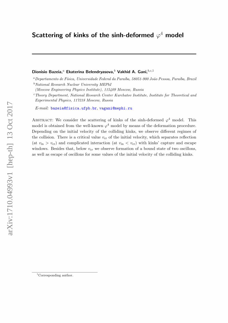
Scattering of kinks of the sinh-deformed ϕ 4 model Dionisio Bazeia, a Ekaterina Belendryasova, b Vakhid A. Gani, b,c,1 a Departamento de F´ ısica, Universidade Federal da Para´ ıba, 58051-900Jo˜aoPessoa, Para´ ıba, Brazil b National Research Nuclear University MEPhI (Moscow Engineering Physics Institute), 115409 Moscow, Russia c Theory Department, National Research Center Kurchatov Institute, Institute for Theoretical and Experimental Physics, 117218 Moscow, Russia E-mail: [email protected], [email protected] Abstract: We consider the scattering of kinks of the sinh-deformed ϕ 4 model. This model is obtained from the well-known ϕ 4 model by means of the deformation procedure. Depending on the initial velocity of the colliding kinks, we observe different regimes of the collision. There is a critical value v cr of the initial velocity, which separates reflection (at v in >v cr ) and complicated interaction (at v in <v cr ) with kinks’ capture and escape windows. Besides that, below v cr we observe formation of a bound state of two oscillons, as well as escape of oscillons for some values of the initial velocity of the colliding kinks. 1 Corresponding author. arXiv:1710.04993v1 [hep-th] 13 Oct 2017
Transcript of Scattering of kinks of the sinh-deformed model · PDF fileScattering of kinks of the...
Scattering of kinks of the sinh-deformed ϕ4 model
Dionisio Bazeia,a Ekaterina Belendryasova,b Vakhid A. Gani,b,c,1
aDepartamento de Fısica, Universidade Federal da Paraıba, 58051-900 Joao Pessoa, Paraıba, BrazilbNational Research Nuclear University MEPhI
(Moscow Engineering Physics Institute), 115409 Moscow, RussiacTheory Department, National Research Center Kurchatov Institute, Institute for Theoretical and
Experimental Physics, 117218 Moscow, Russia
E-mail: [email protected], [email protected]
Abstract: We consider the scattering of kinks of the sinh-deformed ϕ4 model. This
model is obtained from the well-known ϕ4 model by means of the deformation procedure.
Depending on the initial velocity of the colliding kinks, we observe different regimes of
the collision. There is a critical value vcr of the initial velocity, which separates reflection
(at vin > vcr) and complicated interaction (at vin < vcr) with kinks’ capture and escape
windows. Besides that, below vcr we observe formation of a bound state of two oscillons,
as well as escape of oscillons for some values of the initial velocity of the colliding kinks.
1Corresponding author.
arX
iv:1
710.
0499
3v1
[he
p-th
] 1
3 O
ct 2
017
Contents
1 Introduction 1
2 Topological solitons in (1,1)-dimensional models 3
3 The ϕ4 model 6
4 Deformation procedure and the sinh-deformed ϕ4 model 8
5 Kink-antikink collisions in the sinh-deformed ϕ4 model 10
6 Comments and Conclusion 13
1 Introduction
Topological defects arise in a diversity of contexts in high energy physics, cosmology, quan-
tum and classical field theory, condensed matter, and so on. In high energy physics, they are
topologically non-trivial solutions of the equations of motion and possess very interesting
properties, which lead to new physical phenomena [1–4].
Nowadays, the study of the topological defects is a very fast developing area with
significant progress being achieved in the investigation of domain walls, vortices, strings,
as well as embedded topological defects such as Q-lump on a domain wall and skyrmion on a
domain wall, and so on [5–14]. Besides, it is also of interest to mention the so-called Q-balls
and similar configurations [15–20], which are charged and then protected against decaying
into the elementary excitations supported by the model under consideration. Also, it is
worth mentioning other possibilities, such as the study of solitons in fibers [21], bubble
collisions in cosmology [22], and localized excitations in nonlinear systems [23].
The (1, 1)-dimensional models are of special interest [2, 3, 24], since the dynamics of
some two- or three-dimensional systems can be reduced to the one-dimensional models.
For example, a planar domain wall, which separates regions with different minima of the
potential, in the direction perpendicular to it can be interpreted as a one-dimensional topo-
logical configuration (a kink). On the other hand, the (1, 1)-dimensional field-theoretical
models can be a first step toward more complicated higher dimensional models. Moreover,
even in the (1, 1)-dimensional case, topological defects may arise in the more complex mod-
els with two or more fields; see, e.g., refs. [25–51]. In this more general context, several
works have been developed to find analytical solutions, to study their stability and to use
them in application of interest in physics [25–36]. Other investigations have dealt with
the presence of junctions and/or intersections of defects [37–40], and with issues related to
composite-kink internal structures, twinlike models with several fields and triplet scalar on
domain walls [41–51], among other issues.
– 1 –
In the case of models described by real scalar fields with standard kinematics, in the
(1, 1) space-time the presence of interactions that develop spontaneous symmetry breaking
in general leads to localized topological structures having the kinklike profile. The inter-
actions of these one-dimensional topological structures with each other and with spatial
inhomogeneities (impurities) have attracted the attention of physicists and mathematicians
during a long time; see, e.g., ref. [24]. The first studies on this subject date back to the
1970s and 1980s [52, 53]. Nevertheless, forty years later we see that it is still an actively
developing area with many new applications. Many important results have been obtained
by means of the numerical simulation, which is one of the most powerful tools for studying
the subject. In particular, resonance phenomena – escape windows and quasi-resonances –
were found in the kink-antikink scattering process. A broad class of the (1, 1)-dimensional
models with polynomial potentials such as the ϕ4, ϕ6, ϕ8, and others with polynomial
self-interaction with higher degree has been considered [53–66]. Also, one should mention
the new results on the long-range interaction between kinks [65–69]. Other models with
non-polynomial potentials are also being discussed in the literature. For example, the mod-
ified sine-Gordon [70], the double sine-Gordon [71–73], and a variety of models which can
be obtained using the deformation procedure, which we explain below.
Apart from the numerical solving of the equation of motion, other methods are widely
used for investigating the kink-antikink interactions. One of them is the collective co-
ordinate method [55, 74–80]. Within this approximation a real field-theoretical system
(which formally has an infinite number of degrees of freedom) is approximately described
as a system with one or several degrees of freedom. For example, in the case of the kink-
antikink configuration one can use the distance between the kink and the antikink as the
only degree of freedom (collective coordinate). In more complicated modifications of this
approximation some other degrees of freedom (for instance, vibrational) can be involved,
see, e.g., [74–76]. Another approximation, which allows to estimate the force between kink
and antikink, is Manton’s method [3, Ch. 5], [81–84]. This method is based on using the
kinks’ asymptotics in situations where the distance between kinks is large. However, one
should mention that the applicability of this method for kinks and solitons with power-law
asymptotics is not obvious.
An impressive progress has been achieved in the analytical treatment of the (1, 1)-
dimensional field-theoretical models. Among several possibilities to deal with the problem
analytically, the trial orbit method was suggested in [25] as a way to solve the equations of
motion which appear in systems described by two real scalar fields that interact nonlinearly.
This method has been used by others, and in [43] it was shown to be very effective when
the equations of motion can be reduced to first-order differential equations. Also, in [44]
the authors have used the integrating factor to solve the equations of motion in the case
of a very specific potential.
Another possibility of searching for models that support analytical solutions appeared
before in [85] and also in refs. [86–88]. It refers to the deformation procedure, a method
of current interest which helps us to introduce new models, and solve them analytically.
This will be further reviewed below, and used to define the model we want to investigate
in the current work. In particular, the new model is somehow similar to the ϕ4 model with
– 2 –
spontaneous symmetry breaking, so we will compare the current investigation with the ϕ4
case, to highlight the differences between the two cases, and to see how the non-polynomial
interaction that appears in the new model contributes to modify the behavior which is
present in the standard ϕ4 model.
In this work we focus our attention on the kink-antikink scattering process and orga-
nize the investigation as follows. In section 2 we give general introduction to the (1, 1)-
dimensional field-theoretical models, which possess topological solutions with the kink pro-
file. In section 3 we review the ϕ4 model, briefly accounting for the kink-antikink scattering
within this model. Furthermore, in section 4 we apply the deformation procedure to the
ϕ4 model in order to introduce a model with non-polynomial potential, which we call the
sinh-deformed ϕ4 model. In section 5 we focus on the collisions of the kink and the antikink
of the sinh-deformed ϕ4 model. In this section we present our main results and compare
them with the results of the ϕ4 model. Finally, in section 6 we conclude with a discussion
of the results and the prospects for future works.
2 Topological solitons in (1,1)-dimensional models
Consider a field-theoretical model in the (1, 1)-dimensional space-time with its dynamics
defined by the Lagrangian
L =1
2
(∂ϕ
∂t
)2
− 1
2
(∂ϕ
∂x
)2
− U(ϕ), (2.1)
where ϕ(x, t) is a real scalar field. The potential U(ϕ) is supposed to be non-negative func-
tion with two or more degenerate minima, ϕ(0)1 , ϕ
(0)2 , . . . , such that U(ϕ
(0)1 ) = U(ϕ
(0)2 ) =
... = 0. The Lagrangian (2.1) leads to the following equation of motion for the field ϕ
∂2ϕ
∂t2− ∂2ϕ
∂x2+dU
dϕ= 0. (2.2)
The energy functional corresponding to the Lagrangian (2.1) is
E[ϕ] =
∫ ∞−∞
[1
2
(∂ϕ
∂t
)2
+1
2
(∂ϕ
∂x
)2
+ U(ϕ)
]dx. (2.3)
In the static case∂ϕ
∂t= 0, and from eq. (2.2) we have
d2ϕ
dx2=dU
dϕ. (2.4)
This equation can be easily transformed into the first order differential equations
dϕ
dx= ±√
2U. (2.5)
For the energy of the static configuration to be finite, the two following conditions must
hold
limx→−∞
ϕ(x) = ϕ(0)i and lim
x→+∞ϕ(x) = ϕ
(0)j , (2.6)
– 3 –
where ϕ(0)i and ϕ
(0)j are two adjacent minima of the potential. These expressions (2.6) are
necessary conditions for the energy of a static configuration to be finite. If (2.6) hold, then
the second and the third terms in the integrand in (2.3) fall off at x → ±∞, hence the
integral (2.3) can be convergent. Configurations with ϕ(0)i 6= ϕ
(0)j are called topological and
have a kinklike shape. In this sense, a conserved topological current can be introduced,
and for the models to be investigated below one can use
jµtop =1
2εµν∂νϕ. (2.7)
The corresponding topological charge is
Qtop =
∫ ∞−∞
j0topdx =
1
2[ϕ(+∞)− ϕ(−∞)] . (2.8)
This charge is determined only by the asymptotics (2.6), so it does not depend on the
behavior of the field ϕ(x) at finite x.
For every non-negative potential U(ϕ) we can introduce a smooth function W (ϕ),
called the superpotential, as
U(ϕ) =1
2
(dW
dϕ
)2
. (2.9)
Using the superpotential we can rewrite the energy of a static configuration ϕ(x) in the
following manner
E = EBPS +1
2
∫ ∞−∞
(dϕ
dx± dW
dϕ
)2
dx, (2.10)
where
EBPS = |W [ϕ(+∞)]−W [ϕ(−∞)]|. (2.11)
From eq. (2.10) one can see that the energy of any static configuration belonging to a given
topological sector is bounded from below by EBPS. The configurations with the minimal
energy (2.11) are called BPS configurations, or BPS saturated configurations [89, 90]. From
eq. (2.10) it is easy to see that any BPS configuration satisfies the first order differential
equationsdϕ
dx= ±dW
dϕ, (2.12)
which coincide with (2.5).
Below we deal with kinks and antikinks — the BPS saturated topological solutions
of eq. (2.5), which interpolate between neighboring minima of the potential. The solution
with the asymptitics ϕ(+∞) > ϕ(−∞) is called kink, while the term antikink stands for
the solution with ϕ(+∞) < ϕ(−∞). Sometimes we use the term kink for both kink and
antikink, for brevity.
Many phenomena observed in the kink-antikink scattering can be explained by the
presence of the vibrational mode(s) in the kink’s excitation spectrum. In order to find the
spectrum of localized excitations of a kink, we have to add a small perturbation δϕ(x, t)
to the static kink solution ϕk(x),
ϕ(x, t) = ϕk(x) + δϕ(x, t), |δϕ| � |ϕk|. (2.13)
– 4 –
The substitution of ϕ(x, t) into the equation of motion (2.2) leads to the partial differential
equation for the perturbation δϕ(x, t); after linearization one gets
∂2δϕ
∂t2− ∂2δϕ
∂x2+d2U
dϕ2
∣∣∣∣ϕk(x)
δϕ = 0. (2.14)
Since the second derivative of the potential calculated at the static solution ϕk(x) depends
only on x, we can assume that δϕ has the form
δϕ(x, t) = η(x) cos ωt, (2.15)
and this allows us to obtain the eigenvalue problem of the type of the stationary Schrodinger
equation,
Hη(x) = ω2η(x), (2.16)
where the operator H (the Hamiltonian) is
H = − d2
dx2+ u(x), (2.17)
with the potential
u(x) =d2U
dϕ2
∣∣∣∣ϕk(x)
. (2.18)
For each state of the discrete spectrum, the corresponding eigenfunction η(x) is a twice
continuously differentiable and square-integrable on the x-axis. Kink and antikink have
the same excitation spectrum.
The discrete spectrum in the potential (2.18) always possesses a zero (or translational)
mode ω0 = 0. It can easily be shown by differentiating eq. (2.4) with respect to x, and
taking into account that ϕk(x) is a solution of eq. (2.4), i.e.
− d2
dx2
dϕk
dx+d2U
dϕ2
∣∣∣∣ϕk(x)
dϕk
dx= 0, or H ·
dϕk
dx= 0. (2.19)
So we see thatdϕk
dxis an eigenfunction of the Hamiltonian (2.17) associated with the
eigenvalue ω0 = 0. The presence of a zero mode in the kink’s excitation spectrum is a
consequence of the translational invariance of the Lagrangian.
Furthermore, the presence of W in eq. (2.9) allows to write the operator H in the form
H = A†A, (2.20)
where A† and A are the first order differential operators
A† = − d
dx+d2W
dϕ2
∣∣∣∣ϕk(x)
, A =d
dx+d2W
dϕ2
∣∣∣∣ϕk(x)
. (2.21)
This factorization shows that the operator H is non-negative, so the static solution ϕk(x)
is linearly stable.
– 5 –
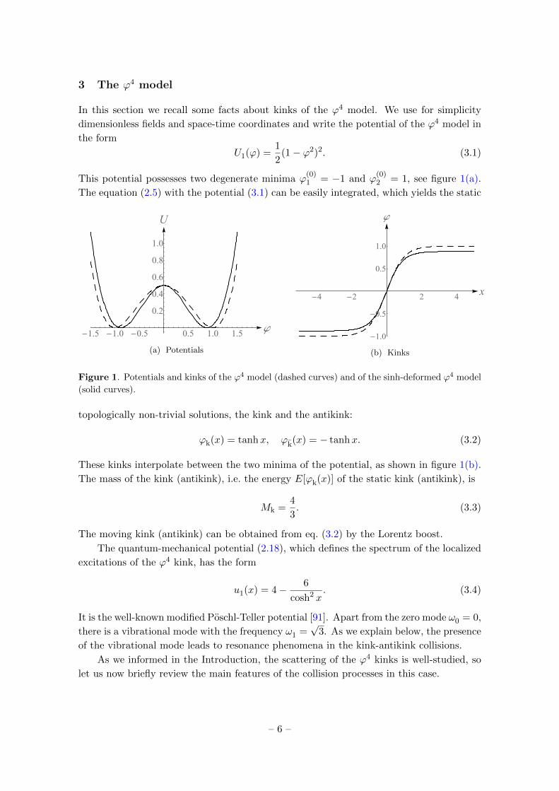
3 The ϕ4 model
In this section we recall some facts about kinks of the ϕ4 model. We use for simplicity
dimensionless fields and space-time coordinates and write the potential of the ϕ4 model in
the form
U1(ϕ) =1
2(1− ϕ2)2. (3.1)
This potential possesses two degenerate minima ϕ(0)1 = −1 and ϕ
(0)2 = 1, see figure 1(a).
The equation (2.5) with the potential (3.1) can be easily integrated, which yields the static
-1.5 -1.0 -0.5 0.5 1.0 1.5 φ
0.2
0.4
0.6
0.8
1.0
U
(a) Potentials
-4 -2 2 4 x
-1.0
-0.5
0.5
1.0
φ
(b) Kinks
Figure 1. Potentials and kinks of the ϕ4 model (dashed curves) and of the sinh-deformed ϕ4 model
(solid curves).
topologically non-trivial solutions, the kink and the antikink:
ϕk(x) = tanhx, ϕk(x) = − tanhx. (3.2)
These kinks interpolate between the two minima of the potential, as shown in figure 1(b).
The mass of the kink (antikink), i.e. the energy E[ϕk(x)] of the static kink (antikink), is
Mk =4
3. (3.3)
The moving kink (antikink) can be obtained from eq. (3.2) by the Lorentz boost.
The quantum-mechanical potential (2.18), which defines the spectrum of the localized
excitations of the ϕ4 kink, has the form
u1(x) = 4− 6
cosh2 x. (3.4)
It is the well-known modified Poschl-Teller potential [91]. Apart from the zero mode ω0 = 0,
there is a vibrational mode with the frequency ω1 =√
3. As we explain below, the presence
of the vibrational mode leads to resonance phenomena in the kink-antikink collisions.
As we informed in the Introduction, the scattering of the ϕ4 kinks is well-studied, so
let us now briefly review the main features of the collision processes in this case.
– 6 –
Consider the initial configuration in the form of kink and antikink centered at the
points x = −x0 and x = x0, respectively, and moving towards each other with the initial
velocities vin in the laboratory frame, i.e.
ϕ(x, t) = tanh
x+ x0 − vint√1− v2
in
− tanh
x− x0 + vint√1− v2
in
− 1. (3.5)
To find evolution of this initial configuration, we solved the equation of motion (2.2) with
the potential (3.1) numerically using the standard explicit finite difference scheme,
∂2ϕ
∂t2=ϕj+1i − 2ϕji + ϕj−1
i
δt2,
∂2ϕ
∂x2=ϕji+1 − 2φji + ϕji−1
δx2, (3.6)
where (i, j) number the x and t coordinates of the grid points, (xi, tj), on a grid with the
steps δt = 0.008 and δx = 0.01. We repeated selected computations with smaller steps,
δt = 0.004 and δx = 0.005, in order to check our numerical results. We also checked the
total energy conservation. In all simulations of the ϕ4 kinks collisions we used the initial
half-distance x0 = 5.
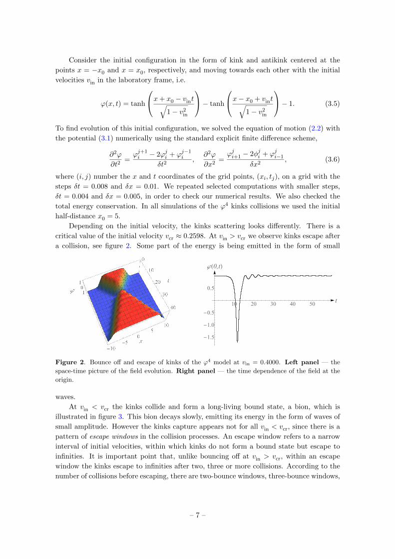
Depending on the initial velocity, the kinks scattering looks differently. There is a
critical value of the initial velocity vcr ≈ 0.2598. At vin > vcr we observe kinks escape after
a collision, see figure 2. Some part of the energy is being emitted in the form of small
10 20 30 40 50t
-1.5
-1.0
-0.5
0.5
φ(0,t)
Figure 2. Bounce off and escape of kinks of the ϕ4 model at vin = 0.4000. Left panel — the
space-time picture of the field evolution. Right panel — the time dependence of the field at the
origin.
waves.
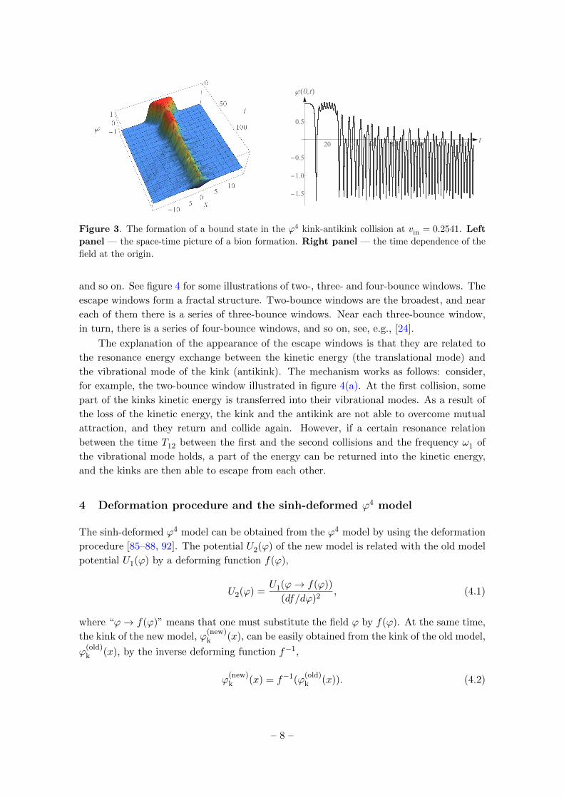
At vin < vcr the kinks collide and form a long-living bound state, a bion, which is
illustrated in figure 3. This bion decays slowly, emitting its energy in the form of waves of
small amplitude. However the kinks capture appears not for all vin < vcr, since there is a
pattern of escape windows in the collision processes. An escape window refers to a narrow
interval of initial velocities, within which kinks do not form a bound state but escape to
infinities. It is important point that, unlike bouncing off at vin > vcr, within an escape
window the kinks escape to infinities after two, three or more collisions. According to the
number of collisions before escaping, there are two-bounce windows, three-bounce windows,
– 7 –
20 40 60 80 100 120 140t
-1.5
-1.0
-0.5
0.5
φ(0,t)
Figure 3. The formation of a bound state in the ϕ4 kink-antikink collision at vin = 0.2541. Left
panel — the space-time picture of a bion formation. Right panel — the time dependence of the
field at the origin.
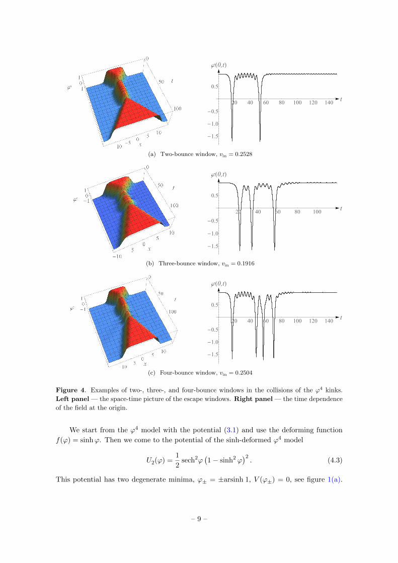
and so on. See figure 4 for some illustrations of two-, three- and four-bounce windows. The
escape windows form a fractal structure. Two-bounce windows are the broadest, and near
each of them there is a series of three-bounce windows. Near each three-bounce window,
in turn, there is a series of four-bounce windows, and so on, see, e.g., [24].
The explanation of the appearance of the escape windows is that they are related to
the resonance energy exchange between the kinetic energy (the translational mode) and
the vibrational mode of the kink (antikink). The mechanism works as follows: consider,
for example, the two-bounce window illustrated in figure 4(a). At the first collision, some
part of the kinks kinetic energy is transferred into their vibrational modes. As a result of
the loss of the kinetic energy, the kink and the antikink are not able to overcome mutual
attraction, and they return and collide again. However, if a certain resonance relation
between the time T12 between the first and the second collisions and the frequency ω1 of
the vibrational mode holds, a part of the energy can be returned into the kinetic energy,
and the kinks are then able to escape from each other.
4 Deformation procedure and the sinh-deformed ϕ4 model
The sinh-deformed ϕ4 model can be obtained from the ϕ4 model by using the deformation
procedure [85–88, 92]. The potential U2(ϕ) of the new model is related with the old model
potential U1(ϕ) by a deforming function f(ϕ),
U2(ϕ) =U1(ϕ→ f(ϕ))
(df/dϕ)2, (4.1)
where “ϕ→ f(ϕ)” means that one must substitute the field ϕ by f(ϕ). At the same time,
the kink of the new model, ϕ(new)k (x), can be easily obtained from the kink of the old model,
ϕ(old)k (x), by the inverse deforming function f−1,
ϕ(new)k (x) = f−1(ϕ
(old)k (x)). (4.2)
– 8 –
20 40 60 80 100 120 140t
-1.5
-1.0
-0.5
0.5
φ(0,t)
(a) Two-bounce window, vin = 0.2528
20 40 60 80 100t
-1.5
-1.0
-0.5
0.5
φ(0,t)
(b) Three-bounce window, vin = 0.1916
20 40 60 80 100 120 140t
-1.5
-1.0
-0.5
0.5
φ(0,t)
(c) Four-bounce window, vin = 0.2504
Figure 4. Examples of two-, three-, and four-bounce windows in the collisions of the ϕ4 kinks.
Left panel — the space-time picture of the escape windows. Right panel — the time dependence
of the field at the origin.
We start from the ϕ4 model with the potential (3.1) and use the deforming function
f(ϕ) = sinhϕ. Then we come to the potential of the sinh-deformed ϕ4 model
U2(ϕ) =1
2sech2ϕ
(1− sinh2 ϕ
)2. (4.3)
This potential has two degenerate minima, ϕ± = ±arsinh 1, V (ϕ±) = 0, see figure 1(a).
– 9 –
The kinks of the sinh-deformed ϕ4 model are
ϕk(x) = arsinh(tanhx), ϕk(x) = −arsinh(tanhx), (4.4)
see figure 1(b). The mass of the sinh-deformed ϕ4 kink (antikink), i.e. the energy E[ϕk(x)]
of the static kink (antikink), is
Mk = π − 2. (4.5)
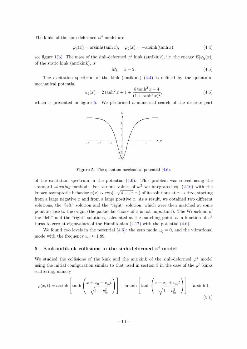
The excitation spectrum of the kink (antikink) (4.4) is defined by the quantum-
mechanical potential
u2(x) = 2 tanh2 x+ 1 +8 tanh2 x− 4
(1 + tanh2 x)2, (4.6)
which is presented in figure 5. We performed a numerical search of the discrete part
-3 -2 -1 1 2 x
-3
-2
-1
1
2
3
u
Figure 5. The quantum-mechanical potential (4.6).
of the excitation spectrum in the potential (4.6). This problem was solved using the
standard shooting method. For various values of ω2 we integrated eq. (2.16) with the
known asymptotic behavior η(x) ∼ exp(−√
4− ω2|x|) of its solutions at x→ ±∞, starting
from a large negative x and from a large positive x. As a result, we obtained two different
solutions, the “left” solution and the “right” solution, which were then matched at some
point x close to the origin (the particular choice of x is not important). The Wronskian of
the “left” and the “right” solutions, calculated at the matching point, as a function of ω2
turns to zero at eigenvalues of the Hamiltonian (2.17) with the potential (4.6).
We found two levels in the potential (4.6): the zero mode ω0 = 0, and the vibrational
mode with the frequency ω1 ≈ 1.89.
5 Kink-antikink collisions in the sinh-deformed ϕ4 model
We studied the collisions of the kink and the antikink of the sinh-deformed ϕ4 model
using the initial configuration similar to that used in section 3 in the case of the ϕ4 kinks
scattering, namely
ϕ(x, t) = arsinh
tanh
x+ x0 − vint√1− v2
in
− arsinh
tanh
x− x0 + vint√1− v2
in
− arsinh 1,
(5.1)
– 10 –
which corresponds to the kink and the antikink centered at x = ±x0 and moving towards
each other with the initial velocities vin. We used 2x0 = 10 and the same parameters of the
numerical scheme as for the ϕ4 kinks in section 3, see eq. (3.6) and the paragraph below
this equation.
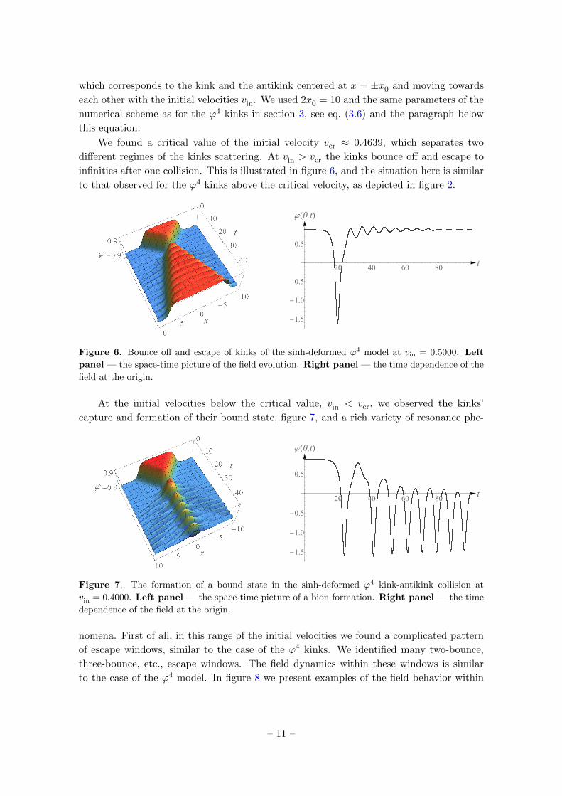
We found a critical value of the initial velocity vcr ≈ 0.4639, which separates two
different regimes of the kinks scattering. At vin > vcr the kinks bounce off and escape to
infinities after one collision. This is illustrated in figure 6, and the situation here is similar
to that observed for the ϕ4 kinks above the critical velocity, as depicted in figure 2.
20 40 60 80t
-1.5
-1.0
-0.5
0.5
φ(0,t)
Figure 6. Bounce off and escape of kinks of the sinh-deformed ϕ4 model at vin = 0.5000. Left
panel — the space-time picture of the field evolution. Right panel — the time dependence of the
field at the origin.
At the initial velocities below the critical value, vin < vcr, we observed the kinks’
capture and formation of their bound state, figure 7, and a rich variety of resonance phe-
20 40 60 80t
-1.5
-1.0
-0.5
0.5
φ(0,t)
Figure 7. The formation of a bound state in the sinh-deformed ϕ4 kink-antikink collision at
vin = 0.4000. Left panel — the space-time picture of a bion formation. Right panel — the time
dependence of the field at the origin.
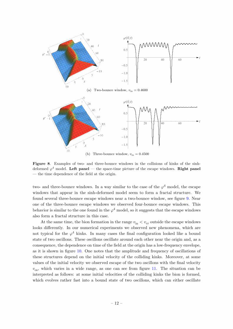
nomena. First of all, in this range of the initial velocities we found a complicated pattern
of escape windows, similar to the case of the ϕ4 kinks. We identified many two-bounce,
three-bounce, etc., escape windows. The field dynamics within these windows is similar
to the case of the ϕ4 model. In figure 8 we present examples of the field behavior within
– 11 –
20 40 60t
-1.5
-1.0
-0.5
0.5
φ(0,t)
(a) Two-bounce window, vin = 0.4600
20 40 60t
-1.5
-1.0
-0.5
0.5
φ(0,t)
(b) Three-bounce window, vin = 0.4500
Figure 8. Examples of two- and three-bounce windows in the collisions of kinks of the sinh-
deformed ϕ4 model. Left panel — the space-time picture of the escape windows. Right panel
— the time dependence of the field at the origin.
two- and three-bounce windows. In a way similar to the case of the ϕ4 model, the escape
windows that appear in the sinh-deformed model seem to form a fractal structure. We
found several three-bounce escape windows near a two-bounce window, see figure 9. Near
one of the three-bounce escape windows we observed four-bounce escape windows. This
behavior is similar to the one found in the ϕ4 model, so it suggests that the escape windows
also form a fractal structure in this case.
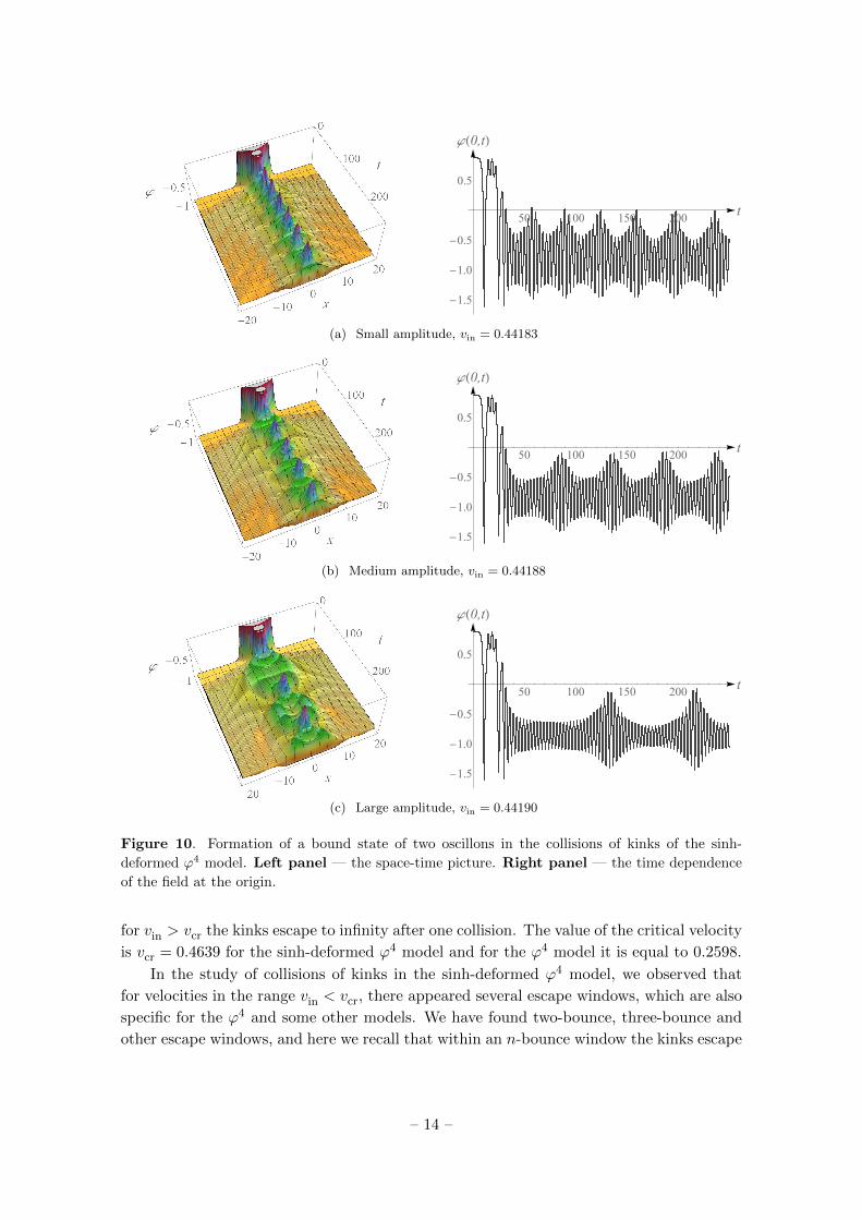
At the same time, the bion formation in the range vin < vcr outside the escape windows
looks differently. In our numerical experiments we observed new phenomena, which are
not typical for the ϕ4 kinks. In many cases the final configuration looked like a bound
state of two oscillons. These oscillons oscillate around each other near the origin and, as a
consequence, the dependence on time of the field at the origin has a low-frequency envelope,
as it is shown in figure 10. One notes that the amplitude and frequency of oscillations of
these structures depend on the initial velocity of the colliding kinks. Moreover, at some
values of the initial velocity we observed escape of the two oscillons with the final velocity
vos, which varies in a wide range, as one can see from figure 11. The situation can be
interpreted as follows: at some initial velocities of the colliding kinks the bion is formed,
which evolves rather fast into a bound state of two oscillons, which can either oscillate
– 12 –
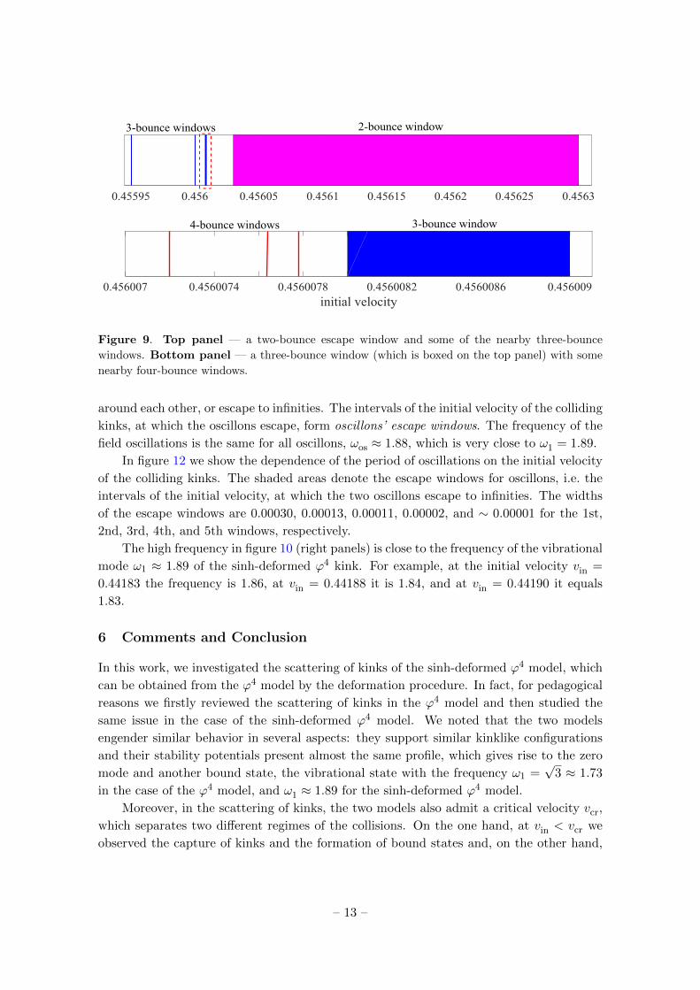
Figure 9. Top panel — a two-bounce escape window and some of the nearby three-bounce
windows. Bottom panel — a three-bounce window (which is boxed on the top panel) with some
nearby four-bounce windows.
around each other, or escape to infinities. The intervals of the initial velocity of the colliding
kinks, at which the oscillons escape, form oscillons’ escape windows. The frequency of the
field oscillations is the same for all oscillons, ωos ≈ 1.88, which is very close to ω1 = 1.89.
In figure 12 we show the dependence of the period of oscillations on the initial velocity
of the colliding kinks. The shaded areas denote the escape windows for oscillons, i.e. the
intervals of the initial velocity, at which the two oscillons escape to infinities. The widths
of the escape windows are 0.00030, 0.00013, 0.00011, 0.00002, and ∼ 0.00001 for the 1st,
2nd, 3rd, 4th, and 5th windows, respectively.
The high frequency in figure 10 (right panels) is close to the frequency of the vibrational
mode ω1 ≈ 1.89 of the sinh-deformed ϕ4 kink. For example, at the initial velocity vin =
0.44183 the frequency is 1.86, at vin = 0.44188 it is 1.84, and at vin = 0.44190 it equals
1.83.
6 Comments and Conclusion
In this work, we investigated the scattering of kinks of the sinh-deformed ϕ4 model, which
can be obtained from the ϕ4 model by the deformation procedure. In fact, for pedagogical
reasons we firstly reviewed the scattering of kinks in the ϕ4 model and then studied the
same issue in the case of the sinh-deformed ϕ4 model. We noted that the two models
engender similar behavior in several aspects: they support similar kinklike configurations
and their stability potentials present almost the same profile, which gives rise to the zero
mode and another bound state, the vibrational state with the frequency ω1 =√
3 ≈ 1.73
in the case of the ϕ4 model, and ω1 ≈ 1.89 for the sinh-deformed ϕ4 model.
Moreover, in the scattering of kinks, the two models also admit a critical velocity vcr,
which separates two different regimes of the collisions. On the one hand, at vin < vcr we
observed the capture of kinks and the formation of bound states and, on the other hand,
– 13 –
50 100 150 200t
-1.5
-1.0
-0.5
0.5
φ(0,t)
(a) Small amplitude, vin = 0.44183
50 100 150 200t
-1.5
-1.0
-0.5
0.5
φ(0,t)
(b) Medium amplitude, vin = 0.44188
50 100 150 200t
-1.5
-1.0
-0.5
0.5
φ(0,t)
(c) Large amplitude, vin = 0.44190
Figure 10. Formation of a bound state of two oscillons in the collisions of kinks of the sinh-
deformed ϕ4 model. Left panel — the space-time picture. Right panel — the time dependence
of the field at the origin.
for vin > vcr the kinks escape to infinity after one collision. The value of the critical velocity
is vcr = 0.4639 for the sinh-deformed ϕ4 model and for the ϕ4 model it is equal to 0.2598.
In the study of collisions of kinks in the sinh-deformed ϕ4 model, we observed that
for velocities in the range vin < vcr, there appeared several escape windows, which are also
specific for the ϕ4 and some other models. We have found two-bounce, three-bounce and
other escape windows, and here we recall that within an n-bounce window the kinks escape
– 14 –
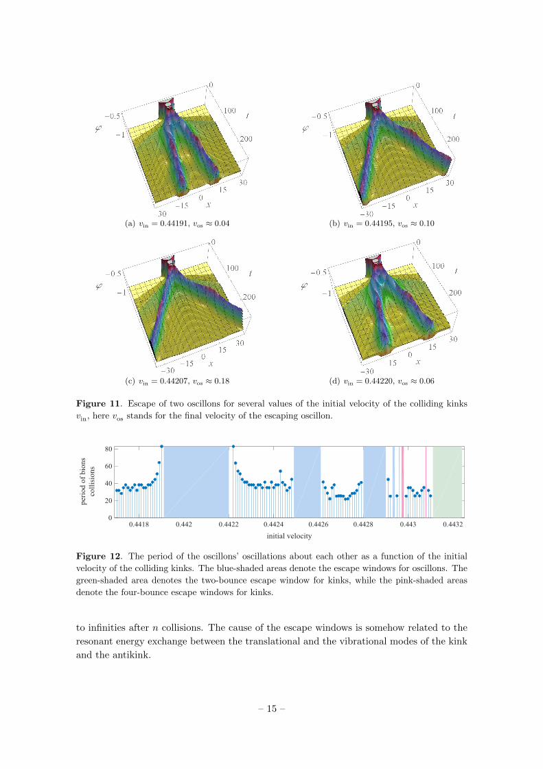
(a) vin = 0.44191, vos ≈ 0.04
(b) vin = 0.44195, vos ≈ 0.10
(c) vin = 0.44207, vos ≈ 0.18
(d) vin = 0.44220, vos ≈ 0.06
Figure 11. Escape of two oscillons for several values of the initial velocity of the colliding kinks
vin, here vos stands for the final velocity of the escaping oscillon.
Figure 12. The period of the oscillons’ oscillations about each other as a function of the initial
velocity of the colliding kinks. The blue-shaded areas denote the escape windows for oscillons. The
green-shaded area denotes the two-bounce escape window for kinks, while the pink-shaded areas
denote the four-bounce escape windows for kinks.
to infinities after n collisions. The cause of the escape windows is somehow related to the
resonant energy exchange between the translational and the vibrational modes of the kink
and the antikink.
– 15 –
The general results of the kink collisions which appear in the sinh-deformed model
suggest that the model is not integrable, and that its kinklike configuration is not a soliton.
This is of current interest, and we may make it stronger if one recalls the sine-Gordon model,
which is integrable model [93]. It is interesting to see that this model can also be obtained
from the ϕ4 model with the deformation procedure. We use the deformation function
f(ϕ) = sinϕ, the potential U1(ϕ) in eq. (3.1) and the procedure illustrated in eq. (4.1) to
get
U3(ϕ) =1
2cos2 ϕ. (6.1)
This is the potential of the sine-Gordon model, and its kinklike or better soliton solution
can be written in the form
ϕs(x) = arcsin(tanhx). (6.2)
As it is well-known, the corresponding stability potential supports the zero mode and no
other bound state, and this helps us to understand its integrability. The sine-Gordon
potential is periodic and so well-different from the ϕ4 model, which is described by a
polynomial potential. In this sense, the sinh-deformed model which we have studied in this
work seems to be farther away from the sine-Gordon and integrability, and hence it should
present information that is absent in the ϕ4 model.
With this motivation in mind, we then looked deeper into the escape windows in the
sinh-deformed model and observed a new phenomenon, the conversion of the kink-antikink
pair into a complex oscillating structure at the collision point at the origin. This structure
can be interpreted as a bound state of two individual oscillons. It is interesting that at
some initial velocities of the colliding kinks we observed escape of these two oscillons.
The interval of initial velocities of the kinks, in which the kinks collide and form a
bound state of two oscillons, which then escape, can be called an oscillons’ escape window.
In our simulations the final velocity of the escaping oscillons varies in a wide range from
zero to ∼ 0.2. Near the oscillons’ escape window the period of the oscillons’ oscillations in
their bound state increases, see figure 12.
As shown in the recent work [92], we can introduce other models using the deformation
function of the hyperbolic type. In particular, we can start with the ϕ6 model studied before
in [54], which supports no vibrational state. For instance, we can use the potential
U4(ϕ) =1
2ϕ2(1− ϕ2)2, (6.3)
and the deformation function f(ϕ) = sinhϕ to get to a new model
U5(ϕ) =1
2tanh2 ϕ (1− sinhϕ)2. (6.4)
We note that for ϕ very small, the above model (6.4) leads us back to the model in (6.3). We
call this model (6.4) the sinh-deformed ϕ6 model. An interesting issue would be to study
the scattering of kinks in this model, to see how it can be connected to the investigation
[54–57], which revealed a resonant scattering structure that provided a counterexample to
the belief that the existence of the vibrational bound state is a necessary condition for the
– 16 –
appearance of multibounce resonances. Another issue is the study of the force between
kinks, to see if it can be connected with the scattering of kinks.
We can also consider models with modified kinematics, as the ones recently investigated
in [94], where one considers the Dirac-Born-Infeld case. This modification changes the
standard scenario and may contribute to add new possibilities to the escape windows that
appear in the standard situation. Another route concerns models described by two real
scalar fields, as the one investigated in refs. [29, 41]. In this case, the presence of the two
fields leads to analytical kinklike solutions which have internal structure that can be used
to model Bloch walls. The scenario here is richer and an interesting issue would be the
study of the scattering of kinks in this model, to see how the internal structure contributes
to the presence of the escape windows, etc. These and other similar issues are currently
under consideration, and we hope to report on them in the near future.
Acknowledgments
This work was performed using resources of NRNU MEPhI high-performance comput-
ing center. The research was supported by the Brazilian agency CNPq under contracts
455931/2014-3 and 306614/2014-6, and by the MEPhI Academic Excellence Project under
contract No. 02.a03.21.0005, 27.08.2013.
References
[1] R. Rajaraman, Solitons and Instantons: An Introduction to Solitons and Instantons in
Quantum Field Theory, North-Holland, Amsterdam (1982).
[2] A. Vilenkin and E.P.S. Shellard, Cosmic Strings and Other Topological Defects, Cambridge
University Press, Cambridge U.K. (2000).
[3] N. Manton and P. Sutcliffe, Topological Solitons, Cambridge University Press, Cambridge
U.K. (2004).
[4] T. Vachaspati, Kinks and Domain Walls: An Introduction to Classical and Quantum
Solitons, Cambridge University Press, Cambrifge U.K. (2006).
[5] M. Nitta, Matryoshka Skyrmions, Nucl. Phys. B 872 (2013) 62 [arXiv:1211.4916].
[6] M. Kobayashi and M. Nitta, Sine-Gordon kinks on a domain wall ring, Phys. Rev. D 87
(2013) 085003 [arXiv:1302.0989].
[7] P. Jennings and P. Sutcliffe, The dynamics of domain wall Skyrmions, J. Phys. A 46
(2013) 465401 [arXiv:1305.2869].
[8] S.B. Gudnason and M. Nitta, Domain wall Skyrmions, Phys. Rev. D 89 (2014) 085022
[arXiv:1403.1245].
[9] N. Blyankinshtein, Q-lumps on a domain wall with a spin-orbit interaction, Phys. Rev. D
93 (2016) 065030 [arXiv:1510.07935].
[10] A.Yu. Loginov, Q kink of the nonlinear O(3) σ model involving an explicitly broken
symmetry, Phys. Atom. Nucl. 74 (2011) 740 [Yad. Fiz. 74 (2011) 766].
– 17 –
[11] V.A. Gani, V.G. Ksenzov and A.E. Kudryavtsev, Example of a self-consistent solution for a
fermion on domain wall, Phys. Atom. Nucl. 73 (2010) 1889 [Yad. Fiz. 73 (2010) 1940]
[arXiv:1001.3305].
[12] V.A. Gani, V.G. Ksenzov and A.E. Kudryavtsev, Stable branches of a solution for a
fermion on domain wall, Phys. Atom. Nucl. 74 (2011) 771 [Yad. Fiz. 74 (2011) 797]
[arXiv:1009.4370].
[13] D. Bazeia, A. Mohammadi, Fermionic bound states in distinct kinklike backgrounds,
Eur. Phys. J. C 77 (2017) 203 [arXiv:1702.00891].
[14] D. Bazeia, A. Mohammadi and D.C. Moreira, Fermion bound states in geometrically
deformed backgrounds, arXiv:1706.04406.
[15] M. Cantara, M. Mai and P. Schweitzer, The energy-momentum tensor and D-term of
Q-clouds, Nucl. Phys. A 953 (2016) 1 [arXiv:1510.08015].
[16] I.E. Gulamov, E.Ya. Nugaev and M.N. Smolyakov, Analytic Q-ball solutions and their
stability in a piecewise parabolic potential, Phys. Rev. D 87 (2013) 085043
[arXiv:1303.1173].
[17] D. Bazeia, M.A. Marques and R. Menezes, Exact solutions, energy and charge of stable
Q-balls, Eur. Phys. J. C 76 (2016) 241 [arXiv:1512.04279].
[18] D. Bazeia, L. Losano, M.A. Marques, R. Menezes and R. da Rocha, Compact Q-balls,
Phys. Lett. B 758 (2016) 146 [arXiv:1604.08871].
[19] D. Bazeia, L. Losano, M.A. Marques and R. Menezes, Split Q-balls, Phys. Lett. B 765
(2017) 359 [arXiv:1612.04442].
[20] V. Dzhunushaliev, A. Makhmudov and K.G. Zloshchastiev, Singularity-free model of
electrically charged fermionic particles and gauged Q-balls, Phys. Rev. D 94 (2016) 096012
[arXiv:1611.02105].
[21] Y.S. Kivshar and G. Agrawal, Optical Solitons: From Fibers to Photonic Crystals,
Academic Press, New York (2003).
[22] A. Aguirre and M. C. Johnson, A status report on the observability of cosmic bubble
collisions, Rep. Prog. Phys. 74 (2011) 074901 [arXiv:0908.4105].
[23] B. Malomed (ed.) Spontaneous Symmetry Breaking, Self-Trapping, and Josephson
Oscillations, Springer (2016).
[24] T.I. Belova and A.E. Kudryavtsev, Solitons and their interactions in classical field theory,
Phys. Usp. 40 (1997) 359 [Usp. Fiz. Nauk 167 (1997) 377].
[25] R. Rajaraman, Solitons of Coupled Scalar Field Theories in Two-dimensions,
Phys. Rev. Lett. 42 (1979) 200.
[26] H.M. Ruck, Solitons in Cyclic Symmetric Field Theories, Nucl. Phys. B 167 (1980) 320.
[27] R. MacKenzie, Topological Structures On Domain Walls, Nucl. Phys. B 303 (1988) 149.
[28] E.R.C. Abraham and P.K. Townsend, Intersecting extended objects in supersymmetric field
theories, Nucl. Phys. B 351 (1991) 313.
[29] D. Bazeia, M.J. dos Santos and R.F. Ribeiro, Solitons in systems of coupled scalar fields,
Phys. Lett. A 208 (1995) 84 [hep-th/0311265].
– 18 –
[30] J.R. Morris, Superconducting domain walls from a supersymmetric action, Phys. Rev. D 52
(1995) 1096.
[31] D. Bazeia and M.M. Santos, Classical stability of solitons in systems of coupled scalar fields,
Phys. Lett. A 217 (1996) 28.
[32] D. Bazeia, R.F. Ribeiro and M.M. Santos, Solitons in a class of systems of two coupled real
scalar fields, Phys. Rev. E 54 (1996) 2943.
[33] B. Chibisov and M. Shifman, BPS saturated walls in supersymmetric theories, Phys. Rev. D
56 (1997) 7990 [Erratum: Phys. Rev. D 58 (1998) 109901] [hep-th/9706141]
[34] J.R. Morris, Nested domain defects, Int. J. Mod. Phys. A 13 (1998) 1115 [hep-ph/9707519].
[35] J.D. Edelstein, M.L. Trobo, F.A. Brito and D. Bazeia, Kinks inside supersymmetric domain
ribbons, Phys. Rev. D 57 (1998) 7561 [hep-th/9707016].
[36] D. Bazeia, H. Boschi-Filho and F.A. Brito, Domain defects in systems of two real scalar
fields, JHEP 04 (1999) 028 [hep-th/9811084].
[37] G.W. Gibbons and P.K. Townsend, A Bogomolny equation for intersecting domain walls,
Phys. Rev. Lett. 83 (1999) 1727 [hep-th/9905196].
[38] H. Oda, K. Ito, M. Naganuma and N. Sakai, An Exact solution of BPS domain wall
junction, Phys. Lett. B 471 (1999) 140 [hep-th/9910095].
[39] S.M. Carroll, S. Hellerman and M. Trodden, Domain wall junctions are 1/4 - BPS states,
Phys. Rev. D 61 (2000) 065001 [hep-th/9905217].
[40] D. Bazeia and F.A. Brito, Tiling the plane without supersymmetry, Phys. Rev. Lett. 84
(2000) 1094 [hep-th/9908090].
[41] D. Bazeia and F.A. Brito, Entrapment of a network of domain walls, Phys. Rev. D 62
(2000) 101701 [hep-th/0005045].
[42] V.A. Lensky, V.A. Gani and A.E. Kudryavtsev, Domain walls carrying a U(1) charge,
Sov. Phys. JETP 93 (2001) 677 [Zh. Eksp. Teor. Fiz. 120 (2001) 778] [hep-th/0104266].
[43] D. Bazeia, W. Freire, L. Losano and R.F. Ribeiro, Topological defects and the trial orbit
method, Mod. Phys. Lett. A 17 (2002) 1945 [hep-th/0205305].
[44] A. Alonso Izquierdo, M.A. Gonzalez Leon and J. Mateos Guilarte, The Kink variety in
systems of two coupled scalar fields in two space-time dimensions, Phys. Rev. D 65 (2002)
085012 [hep-th/0201200].
[45] V.A. Gani, N.B. Konyukhova, S.V. Kurochkin and V.A. Lensky, Study of stability of a
charged topological soliton in the system of two interacting scalar fields,
Comput. Math. Math. Phys. 44 (2004) 1968 [Zh. Vychisl. Mat. Mat. Fiz. 44 (2004) 2069]
[arXiv: 0710.2975].
[46] A. Alonso-Izquierdo, D. Bazeia, L. Losano and J. Mateos Guilarte, New Models for Two
Real Scalar Fields and Their Kink-Like Solutions, Adv. High Energy Phys. 2013 (2013)
183295 [arXiv:1308.2724].
[47] D. Bazeia, A.S. Lobao Jr., L. Losano and R. Menezes, First-order formalism for twinlike
models with several real scalar fields, Eur. Phys. J. C 74 (2014) 2755 [arXiv:1312.1198].
[48] H. Katsura, Composite-kink solutions of coupled nonlinear wave equations, Phys. Rev. D 89
(2014) 085019 [arXiv:1312.4263].
– 19 –
[49] V.A. Gani, M.A. Lizunova and R.V. Radomskiy Scalar triplet on a domain wall: an exact
solution, JHEP 04 (2016) 043 [arXiv:1601.07954].
[50] V.A. Gani, M.A. Lizunova and R.V. Radomskiy, Scalar triplet on a domain wall, J. Phys.:
Conf. Ser. 675 (2016) 012020 [arXiv:1602.04446].
[51] S. Akula, C. Balazs and G.A. White, Semi-analytic techniques for calculating bubble wall
profiles, Eur. Phys. J. C 76 (2016) 681 [arXiv:1608.00008].
[52] A.E. Kudryavtsev, Solitonlike solutions for a Higgs scalar field, JETP Lett. 22 (1975) 82
[Pis’ma v ZhETF 22 (1975) 178].
[53] D.K. Campbell, J.F. Schonfeld and C.A. Wingate, Resonance structure in kink-antikink
interactions in ϕ4 theory, Physica D 9 (1983) 1.
[54] M.A. Lohe, Soliton structures in P (ϕ)2, Phys. Rev. D 20 (1979) 3120.
[55] V.A. Gani, A.E. Kudryavtsev and M.A. Lizunova, Kink interactions in the
(1+1)-dimensional ϕ6 model, Phys. Rev. D 89 (2014) 125009 [arXiv:1402.5903].
[56] A. Moradi Marjaneh, V.A. Gani, D. Saadatmand, S.V. Dmitriev and K. Javidan, Multi-kink
collisions in the φ6 model, JHEP 07 (2017) 028 [arXiv:1704.08353].
[57] P. Dorey, K. Mersh, T. Romanczukiewicz and Y. Shnir, Kink-Antikink Collisions in the φ6
Model, Phys. Rev. Lett. 107 (2011) 091602 [arXiv:1101.5951].
[58] A. Khare, I.C. Christov and A. Saxena, Successive phase transitions and kink solutions in
φ8, φ10, and φ12 field theories, Phys. Rev. E 90 (2014) 023208 [arXiv:1402.6766].
[59] V.A. Gani, V. Lensky and M.A. Lizunova, Kink excitation spectra in the (1+1)-dimensional
ϕ8 model, JHEP 08 (2015) 147 [arXiv:1506.02313].
[60] V.A. Gani, V. Lensky, M.A. Lizunova and E.V. Mrozovskaya, Excitation spectra of solitary
waves in scalar field models with polynomial self-interaction, J. Phys.: Conf. Ser. 675
(2016) 012019 [arXiv:1602.02636].
[61] H. Weigel, Emerging Translational Variance: Vacuum Polarization Energy of the ϕ6 kink,
Adv. High Energy Phys. 2017 (2017) 1486912 [arXiv:1706.02657].
[62] H. Weigel, Vacuum polarization energy for general backgrounds in one space dimension,
Phys. Lett. B 766 (2017) 65 [arXiv:1612.08641].
[63] P. Dorey et al., Boundary scattering in the φ4 model, JHEP 05 (2017) 107
[arXiv:1508.02329].
[64] D. Bazeia, M.A. Gonzalez Leon, L. Losano and J. Mateos Guilarte, Deformed defects for
scalar fields with polynomial interactions, Phys. Rev. D 73 (2006) 105008
[hep-th/0605127].
[65] R.V. Radomskiy, E.V. Mrozovskaya, V.A. Gani and I.C. Christov, Topological defects with
power-law tails, J. Phys.: Conf. Ser. 798 (2017) 012087 [arXiv:1611.05634].
[66] E. Belendryasova and V.A. Gani, Scattering of the ϕ8 kinks with power-law asymptotics,
arXiv:1708.00403.
[67] L.E. Guerrero, E.Lopez-Atencio and J.A. Gonzalez, Long-range self-affine correlations in a
random soliton gas, Phys. Rev. E 55 (1997) 7691.
[68] B.A. Mello, J.A. Gonzalez, L.E. Guerrero and E. Lopez-Atencio, Topological defects with
long-range interactions, Phys. Lett. A 244 (1998) 277.
– 20 –
[69] L.E. Guerrero and J.A. Gonzalez, Long-range interacting solitons: pattern formation and
nonextensive thermostatistics, Physica A 257 (1998) 390 [arXiv:patt-sol/9905010].
[70] M. Peyrard and D.K. Campbell, Kink-antikink interactions in a modified sine-Gordon
model, Physica D 9 (1983) 33.
[71] D.K. Campbell, Solitary wave collisions revisited, Physica D 18 (1986) 47.
[72] D.K. Campbell, Kink-antikink interactions in the double sine-Gordon equation, Physica D
19 (1986) 165.
[73] V.A. Gani and A.E. Kudryavtsev, Kink-antikink interactions in the double sine-Gordon
equation and the problem of resonance frequencies, Phys. Rev. E 60 (1999) 3305
[cond-mat/9809015].
[74] H. Weigel, Kink-Antikink Scattering in ϕ4 and φ6 Models, J. Phys.: Conf. Ser. 482 (2014)
012045 [arXiv:1309.6607].
[75] I. Takyi and H. Weigel, Collective coordinates in one-dimensional soliton models revisited,
Phys. Rev. D 94 (2016) 085008 [arXiv:1609.06833].
[76] A. Demirkaya et al., Kink Dynamics in a Parametric φ6 System: A Model With
Controllably Many Internal Modes, arXiv:1706.01193.
[77] H.E. Baron, G. Luchini and W.J. Zakrzewski, Collective coordinate approximation to the
scattering of solitons in the (1+1) dimensional NLS model, J. Phys. A: Math. and Theor.
47 (2014) 265201 [arXiv:1308.4072].
[78] K. Javidan, Collective coordinate variable for soliton-potential system in sine-Gordon
model, J. Math. Phys. 51 (2010) 112902 [arXiv:0910.3058].
[79] I. Christov and C.I. Christov, Physical dynamics of quasi-particles in nonlinear wave
equations, Phys. Lett. A 372 (2008) 841 [nlin/0612005].
[80] V.A. Gani and A.E. Kudryavtsev, Collisions of domain walls in a supersymmetric model,
Phys. Atom. Nucl. 64 (2001) 2043 [Yad. Fiz. 64 (2001) 2130] [hep-th/9904209,
hep-th/9912211].
[81] J.K. Perring and T.H.R. Skyrme, A model unified field equation, Nucl. Phys 31 (1962) 550.
[82] R. Rajaraman, Intersoliton forces in weak-coupling quantum field theories, Phys. Rev. D 15
(1977) 2866.
[83] N.S. Manton, An effective Lagrangian for solitons, Nucl. Phys. B 150 (1979) 397.
[84] P.G. Kevrekidis, A. Khare and A. Saxena, Solitary wave interactions in dispersive equations
using Manton’s approach, Phys. Rev. E 70 (2004) 057603 [nlin/0410045].
[85] D. Bazeia, L. Losano and J.M.C. Malbouisson, Deformed defects, Phys. Rev. D 66 (2002)
101701 [hep-th/0209027].
[86] C.A. Almeida, D. Bazeia, L. Losano and J.M.C. Malbouisson, New results for deformed
defects, Phys. Rev. D 69 (2004) 067702 [hep-th/0405238].
[87] D. Bazeia and L. Losano, Deformed defects with applications to braneworlds, Phys. Rev. D
73 (2006) 025016 [hep-th/0511193].
[88] D. Bazeia, M.A. Gonzalez Leon, L. Losano, and J. Mateos Guilarte, Deformed defects for
scalar fields with polynomial interactions, Phys. Rev. D 73 (2006) 105008
[hep-th/0605127].
– 21 –
[89] E.B. Bogomolny, Stability of Classical Solutions, Sov. J. Nucl. Phys. 24 (1976) 449
[Yad. Fiz. 24 (1976) 861].
[90] M.K. Prasad and C.M. Sommerfield, Exact Classical Solution for the ’t Hooft Monopole and
the Julia-Zee Dyon, Phys. Rev. Lett. 35 (1975) 760.
[91] P.M. Morse and H. Feshbach, Methods of Theoretical Physics, McGraw-Hill Book Co., New
York (1953).
[92] D. Bazeia, E.E.M. Lima and L. Losano, Kinks and branes in models with hyperbolic
interactions, Int. J. Mod. Phys. A 32 (2017) 1750163 [arXiv:1705.02839].
[93] J. Cuevas-Maraver, P. Kevrekidis and F. Williams (eds.) The sine-Gordon model and its
applications, Springer International Publishing, Switzerland (2014).
[94] D. Bazeia, E.E.M. Lima and L. Losano, Kinklike structures in models of the
Dirac-Born-Infeld type, [arXiv:1708.08512].
– 22 –