Scalar Field Theory - University of Oklahoma Physics ...milton/p6433/chap3.pdf · SCALAR FIELD...

Chapter 3

Scalar Field Theory

3.1 Canonical Formulation

The dispersion relation for a particle of mass m is

E2 = p2 + m2, p2 = p · p, (3.1)

or, in relativistic notation, with p0 = E,

0 = pµpµ + m2 ≡ p2 + m2. (3.2)

A wave equation corresponding to this relation is

(−∂2 + m2)φ(x) = 0, (3.3)

which is solved by a plane wave,

φ(x) = eipµxµ = eip·x, p2 + m2 = 0, (3.4)

where we have introduced the scalar product

p · x = pµxµ = p · x − p0t. (3.5)

A Lagrange density which leads to this wave equation is

L(x) = −1

2

(

∂µφ∂µφ + m2φ2)

=1

2

(

φ̇2 − ∇φ · ∇φ − m2φ2)

. (3.6)

The canonical momentum density is

π(x) =∂L

∂φ̇(x)= φ̇(x), (3.7)

31 Version of October 26, 2009

32 Version of October 26, 2009 CHAPTER 3. SCALAR FIELD THEORY

which means that the Hamiltonian density is

H = πφ̇ − L =1

2π2 +

1

2(∇φ)

2+

1

2m2φ2. (3.8)

As in the previous chapter, it is worthwhile to make a decomposition of φinto creation and annihilation operators,

φ(x, t) =

∫

(dk)

(2π)31

2ωk

[

ak(t)eik·x + a†

k(t)e−ik·x

]

=

∫

(dk)

(2π)31

2ωk

[

ake−iωkteik·x + a†keiωkte−ik·x

]

, (3.9)

whereak = ak(0), ωk = +

√

k2 + m2. (3.10)

Appearing here is a relativistically invariant momentum-space measure,

dk̃ ≡ (dk)

(2π)32ωk=

(dk)

(2π)42πδ(k2 + m2)η(k0), (3.11)

since∫ ∞

−∞

dk0δ((k0)2 − ω2k)η(k0) =

1

2ωk. (3.12)

Thus we may write the plane wave expansion (3.9) of the scalar field as

φ(x) =

∫

dk̃(

ak eik·x + a†k e−ik·x

)

, k0 = ωk. (3.13)

The canonical momentum density is

π(x) = φ̇(x) = −i

∫

dk̃ ωk

(

akeik·x − a†ke−ik·x

)

. (3.14)

Since we must have the following equal-time commutation relations,

[φ(x, t), π(x′, t)] = iδ(x − x′), (3.15a)

[φ(x, t), φ(x′, t)] = 0, (3.15b)

[π(x, t), π(x′, t)] = 0, (3.15c)

the creation and annihilation operators satisfy the following commutation rela-tions

[ak, a†k′ ] = 2ωk(2π)3δ(k − k′), (3.16a)

[ak, ak′ ] = [a†k, a†

k′ ] = 0. (3.16b)

We verify this claim by the following straightforward computations for x0 =x′0 = t:

[φ(x, t), π(x′, t)] = −i

∫

dk̃ dk̃′ ωk′

{

−[ak, a†k′ ]e

ik·x−ik′·x′

+ [a†k, ak′ ]e

−ik·x+ik′·x′

}

= i

∫

(dk)

(2π)31

2

{

eik·(x−x′) + e−ik·(x−x′)}

= iδ(x− x′), (3.17)

3.1. CANONICAL FORMULATION 33 Version of October 26, 2009

while

[φ(x, t), φ(x′, t)] =

∫

dk̃ dk̃′{

[ak, a†k′ ]e

ik·x−ik′·x′

+ [a†k, ak′ ]e

−ik·x+ik′·x′

}

=

∫

dk̃{

eik·(x−x′) − e−ik·(x−x′)}

= 0, (3.18)

because∫

dk̃ →∫

dk̃ when k → −k, and likewise for the π-π commutator.Now the Hamiltonian, from Eq. (3.8), is

H =

∫

(dx)H =

∫

(dx) dk̃ dk̃′

{

− 1

2ωkωk′

(


)

×(

ak′eik′·x − a†

k′e−ik′·x

)

− 1

2k · k′

(


)(

ak′eik′·x − a†

k′e−ik′·x

)

+1

2m2(

akeik·x + a†ke−ik·x

)(

ak′eik′·x + a†

k′e−ik′·x

)

}

. (3.19)

We first note that the quantity∫

(dx) eik·x+ik′ ·x = (2π)3δ(k + k′)e−2iωkt (3.20)

has a vanishing coefficient:(

−1

2ω2

k +1

2k2 +

1

2m2

)

aka−k = 0. (3.21)

The same thing happens with the coefficient of∫

(dx) e−ik·x−ik′ ·x = (2π)3δ(k + k′)e2iωkt. (3.22)

But for the cross terms∫

(dx) eik·x−ik′ ·x = (2π)3δ3(k − k′) (3.23)

has the numerical factor

1

2ω2

k +1

2k2 +

1

2m2 = ω2

k, (3.24)

so the Hamiltonian is simply

H =1

2

∫

dk̃ ωk

(

aka†k + a†

kak

)

. (3.25)

This expresses the Hamiltonian of the system as a sum of harmonic oscillatorenergy operators.


The vacuum state |0〉 is the state of lowest energy; it is the no-particle state,annihilated by all ak:

ak|0〉 = 0, ∀k. (3.26)

It will be a zero-energy state if we normal-order H :

:H : =

∫

dk̃1

2ωk:(aka†

k + a†kak): ≡

∫

dk̃ ωk a†kak, (3.27)

where : . . . : means that we put all annihilation operators to the right of allcreation operators (i.e., forget the commutators). The zero-point energy is thussuppressed. (Yet the zero-point energy has been experimentally observed in theCasimir effect, which is the basis of the van der Waals forces which hold theworld together!)

3.2 Path Integral Formulation

Let us now write down, in analogy to the formula (2.123), the path-integralformulation of the vacuum persistence amplitude for a free scalar field, describedby the Lagrangian (3.6), in the presence of a source K:

〈0, +∞|0,−∞〉K =

∫

[dφ] exp

{

i

∫

(dx)

[

−1

2(∂φ)2 − 1

2m2φ2 + Kφ

]}

= Z0[K], (3.28)

where the notation suggests an analogy (it is deeper than that) with the par-tition function of statistical mechanics. As before, we can actually do the φintegral here. As in Sec. 2.3.1, this is most easily done by introducing a Fouriertransform:

φ(x) =

∫

(dp)

(2π)4eip·xφ(p), (3.29)

so that the action is∫

(dx)

[

−1

2∂µφ∂µφ − 1

2m2φ2 + Kφ

]

=

∫

(dp)

(2π)4φ(−p)

[

−1

2(p2 + m2)

]

φ(p) + K(p)φ(−p)

= −1

2

∫

(dp)

(2π)4

{

[

φ(−p)(p2 + m2) − K(−p)] 1

p2 + m2

[

φ(p)(p2 + m2) − K(p)]

− K(−p)1

p2 + m2K(p)

}

. (3.30)

Again we can shift the integration variable so we can write

Z0[K] =

∫

[dφ]e− i

2

∫

(dp)

(2π)4φ(−p)(p2+m2)φ(p)

ei2

∫

(dp)

(2π)4K(−p)(p2+m2)−1K(p)

= Z0[0] exp

[

i

2

∫

(dp)

(2π)4K(−p)

1

p2 + m2K(p)

]

, (3.31)

3.3. EUCLIDEAN SPACE 35 Version of October 26, 2009

where

Z0[0] = 〈0, +∞|0,−∞〉K=0 = 1. (3.32)

To give meaning to the remaining momentum-space integral, quadratic in K,we note that we should have, once again, inserted a convergence factor:

e−ǫ∫

(dx) 12 φ2

= ei∫

(dx) iǫ2 φ2

, (3.33)

which is equivalent to adding an imaginary part to m2:

m2 → m2 − iǫ. (3.34)

Thus we have, analogously to Eq. (2.112),

Z0[K] = exp

[

i

2

∫

(dp)

(2π)4K(−p)

1

p2 + m2 − iǫK(p)

]

= exp

[

i

2

∫

(dx)(dx′)K(x)∆+(x − x′)K(x′)

]

, (3.35)

where the propagation function (or propagator or Green’s function) is

∆+(x − x′) =

∫

(dp)

(2π)4eip·(x−x′)

p2 + m2 − iǫ. (3.36)

This is often called the Feynman propagator. Note that ∆+ satisfies an inho-mogeneous Klein-Gordon equation,

(−∂2 + m2)∆+(x − x′) = δ(x − x′). (3.37)

3.3 Euclidean Space

Another way to define this propagator is to go into four-dimensional Euclideanspace,

i|x0 − x′0| → |x4 − x′4|. (3.38)

Then, in momentum space, we perform a complex frequency rotation,

−ip0 → p4, (dp) = dp0(dp) → i(dp)E . (3.39)

Then the Minkowski space propagator is related to the corresponding Euclideanone by

∆+(x − x′) → i

∫

(dp)E

(2π)4eipµ(x−x′)µ

pµpµ + m2≡ i∆E(x − x′), (3.40)

where the Euclidean scalar product is, for example,

pµpµ = p21 + p2

2 + p23 + p2

4 ≡ p2E . (3.41)


The corresponding transformation on the configuration-space quantities,

(dx) = dx0 (dx) → −i(dx)E , (∂φ)2 → (∂φ)2E , (3.42)

so the corresponding path integral for the generating function becomes

Z0[K] →∫

[dφ] exp

{

−∫

(dx)E

[

1

2(∂φ)2E +

1

2m2φ2 − Kφ

]}

, (3.43)

or

Z0,E [K] = exp

[

1

2

∫

(dx)E(dx′)EK(x)∆E(x − x′)K(x′)

]

. (3.44)

Let us be more precise. Starting from Eq. (3.36) we carry out the p0 inte-gration:

∫ ∞

−∞

dp0

2π

eip0(x−x′)0

−(p0 − ωp + iǫ)(p0 + ωp − iǫ)=

i

2ωpe−iωp|x

0−x′0|, (3.45)

where ωp = +√

p2 + m2. Here, for (x − x′)0 > 0, we have closed the p0

contour with an infinite semicircle in the upper half plane, encircling the pole atp0 = −ωp + iǫ in a positive sense, while for (x−x′)0 < 0 we close the contour inthe lower half plane, and encircle the pole at p0 = +ωp − iǫ in a negative sense.Thus we find

∆+(x − x′) = ∆+(x′ − x) =

{

i∫

dp̃ eip·(x−x′), (x − x′)0 > 0,

i∫

dp̃ e−ip·(x−x′), (x − x′)0 < 0,(3.46)

where now p0 = −p0 = ωp, and we have noted that∫

(dp) f(p2)eip·(x−x′) =

∫

(dp) f(p2)e−ip·(x−x′). (3.47)

The form of the propagation function exhibited in Eq. (3.46) shows that positivefrequency excitations move forward in time.

We can now perform the Euclidean transformation (3.38), which gives

∆+(x − x′) → i∆E(x − x′) = i

∫

(dp)

(2π)31

2ωpeip·(x−x′)−ωp|x4−x′

4|. (3.48)

But now we use the identity

1

2ωpe−ωp|x4−x′

4| =

∫ ∞

−∞

dp4

2π

eip4(x4−x′

4)

p24 + ω2

p

, (3.49)

which again is easily verified by the residue theorem. Thus we have

∆E(x − x′) =

∫

(dp) dp4

(2π)4eip·(x−x′)+ip4(x4−x′

4)

p24 + p2 + m2

=

∫

(dp)E

(2π)4eip·(x−x′)E

p2E + m2

, (3.50)

3.3. EUCLIDEAN SPACE 37 Version of October 26, 2009

as stated in Eq. (3.40).Of course, we can rotate back,

|x4 − x′4| → i|x0 − x′0|, (3.51)

to recover ∆+, but we can also keep rotating in the same sense:

|x4 − x′4| → −i|x0 − x′0|, (3.52)

so the Euclidean propagator becomes

∆E(x − x′) →∫

(dp)

(2π)31

2ωpeip·(x−x′)+iωp|x

0−x′0|

=

∫

(dp)

(2π)31

2ωpe−ip·(x−x′)+iωp|x

0−x′0|

= i∆−(x − x′), (3.53)

that is,

∆−(x − x′) =

{

−i∫

dp̃ e−ip·(x−x′), (x − x′)0 > 0,

−i∫

dp̃ eip·(x−x′), (x − x′)0 < 0.(3.54)

Since, once again an elementary contour integration yields

∫ ∞

−∞

dp0

2π

eip0(x−x′)0

−p20 + ω2

p + iǫ= − i

2ωpeiωp|x

0−x′0|, (3.55)

we have

∆−(x − x′) = ∆−(x′ − x) =

∫

(dp)

(2π)4eip·(x−x′)

p2 + m2 + iǫ(3.56)

in Minkowski space.It is particularly easy to get explicit limiting forms for the Euclidean prop-

agation function. Let R = |x − x′|, and choose the four-dimensional coordinatesystem so that x − x′ = 0, x4 − x′

4 = R. Then from Eq. (3.48)

∆E(R) =

∫

dp̃ e−ωpR (3.57)

has an integrand which is rotationally invariant in three-dimensions, so

(dp) = 4πp2 dp = 4πp ωp dωp = 4π√

ω2p − m2 ωp dωp, (3.58)

and hence

∆E(R) =1

4π2

∫ ∞

m

dωp

√

ω2p − m2 e−ωpR =

m

4π2RK1(mR), (3.59)

where K1 is the modified Bessel function of order 1. At very small distances,much smaller than the Compton wavelength of the particle, mR ≪ 1, we candrop the mass altogether and get

mR ≪ 1 : ∆E(R) ∼ 1

4π2R2

∫ ∞

0

dxx e−x =1

4π2R2. (3.60)


In the opposite limit of large distances, the Euclidean propagator is exponen-tially small, and most of the contribution to the integral comes from values ofωp near m:

∆E(R) =1

4π2R2

∫ ∞

mR

dx√

x2 − (mR)2 e−x

∼ 1

4π2R2

√2mR

∫ ∞

0

du u1/2e−u−mR

=

√2m

4π2R3/2e−mR Γ

(

3

2

)

, (3.61)

where u = x − mR, or, because Γ(

32

)

= 12

√π,

mR ≫ 1 : ∆E(R) ∼√

2m

(4πR)3/2e−mR. (3.62)

In homework you will derive the limiting behaviors of ∆+.

3.3.1 Unitarity

The vacuum-to-vacuum probability amplitude must have modulus less than orequal to one,

|〈0+|0−〉K |2 ≤ 1. (3.63)

But from Eq. (3.35)

|〈0+|0−〉K |2 = exp

[

−∫

(dx)(dx′)K(x)Im ∆+(x − x′)K(x′)

]

= exp

[

−∫

dp̃ |K(p)|2]

, (3.64)

which follows from Eq. (3.46), so this is less than unity unless K = 0. Note thatthis requirement would not be satisfied if we used ∆− in place of ∆+, becausethe sign of the imaginary part is reversed.

3.4 Interactions

A self-interacting scalar field is described by a Lagrangian

L = −1

2(∂µφ∂µφ + m2φ2) − V (φ). (3.65)

An important, although apparently trivial, example is V (φ) = λφ4, where thecoupling constant is dimensionless. (The dimension of φ is that of mass or oflength−1.) Now we can no longer integrate the vacuum persistence amplitude,

〈0, +∞|0,−∞〉K = Z[K] =

∫

[dφ] exp

[

i

∫

(dx)(L + Kφ)

]

. (3.66)

3.5. GREEN’S FUNCTIONS 39 Version of October 26, 2009

Only approximate techniques exist for finding Z[K], such as perturbation theory,which is based on expanding in powers of the coupling constant λ, which is thentreated as small.

3.5 Green’s Functions

These are the coefficients of K(x1) . . . K(xn) when Z[K] is expanded in a Taylorseries in powers of the source. It is in this sense that Z[K] is a generatingfunction:

Z[K] =∞∑

n=0

in

n!

∫

(dx1) . . . (dxn)K(x1) . . .K(xn)G(n)(x1, . . . , xn), (3.67)

or in terms of functional derivatives,

G(n)(x1, . . . , xn) = (−i)n δn

δK(x1) . . . δK(xn)Z(K]

∣

∣

∣

∣

K=0

. (3.68)

For the free theory, with V = 0, we have from Eq. (3.35)

Z0[K] = exp

[

i

2

∫

(dx)(dx′)K(x)∆+(x − x′)K(x′)

]

=

∞∑

m=0

im

2m

1

m!

∫

(dx1) . . . (dx2m)K(x1) . . . K(x2m)∆+(x1 − x2)

×∆+(x3 − x4) . . . ∆+(x2m−1 − x2m). (3.69)

Thus the odd Green’s functions all vanish,

G(2k+1)0 = 0, (3.70a)

while the first few even Green’s functions are

G(2)(x1, x2) = −i∆+(x1 − x2), (3.70b)

G(4)(x1, x2, x3, x4) = −∆+(x1 − x2)∆+(x3 − x4) − ∆+(x1 − x3)∆+(x2 − x4)

− ∆+(x1 − x4)∆+(x2 − x3), (3.70c)

etc. The factorization of terms suggests that we introduce connected Green’sfunctions by writing

Z[K] = eiW [K], (3.71)

where

iW [K] =

∞∑

n=0

in

n!

∫

(dx1) . . . (dxn)K(x1) . . .K(xn)G(n)c (x1, . . . , xn). (3.72)

For the free theory the only nonvanishing Gc is

G(2)c,0(x1, x2) = −i∆+(x1 − x2). (3.73)

In the following we will use the connected Green’s function exclusively andcorrespondingly will drop the c subscript.


3.6 Feynman Rules for Euclidean λφ4 Theory

We will start from the generating function in Euclidean space, see Eq. (3.43),

ZE [K] =

∫

[dφ] exp

{

−∫

(dx)E

[

1

2(∂φ)2E +

1

2m2φ2 + λφ4 − Kφ

]}

, (3.74)

in terms of the dimensionless coupling constant λ. To get the connected Eu-clidean Green’s function we first write

ZE [K] = eWE [K], (3.75)

in terms of which the connected Green’s functions are obtained by differentia-tion:

G(n)E (x1, . . . , xn) =

δn

δK(x1) . . . δK(xn)WE [K]

∣

∣

∣

∣

K=0

. (3.76)

We can, of course, not calculate G(n)E exactly; we can, however, obtain a series

expansion of G(n)E in powers of λ. The (diagrammatic) technique for calculating

G(n)E is called perturbation theory.

When λ = 0 we have a free theory, for which from Eq. (3.44)

WE,0[K] =1

2

∫

(dx)E(dx′)EK(x)∆E(x − x′)K(x′), (3.77)

where [Eq. (3.50)]

∆E(x − x′) =

∫

(dp)E

(2π)4eip·(x−x′)E

p2E + m2

. (3.78)

so

G(2)E,0(x − x′) =

δ2

δK(x)δK(x′)WE,0[K] = ∆E(x − x′), (3.79)

which is just what is obtained from the result (3.73) by the replacement ∆+ →i∆E , as stated in Eq. (3.40).

The perturbative expansion in λ may be generated by the functional deriva-tive form (henceforward, in this section, we will understand and therefore dropthe E subscript)

Z[K] = exp

[

−∫

(dx)λ

(

δ

δK(x)

)4]

eW0[K], (3.80)

which follows because

δ

δK(x)eW0[K] =

∫

[dφ] φ(x) exp

[

−∫

(dx)

(

1

2(∂φ)2 +

1

2m2φ2 − Kφ

)]

.

(3.81)

3.6. FEYNMAN RULES FOR EUCLIDEAN λφ4 THEORY41 Version of October 26, 2009

Now write

Z[K] = eW0e−W0 exp

[

−∫

(dx)λ

(

δ

δK(x)

)4]

eW0

= eW0

{

1 + e−W0

(

exp

[

−∫

(dx)λ

(

δ

δK(x)

)4]

− 1

)

eW0

}

,(3.82)

or, taking the logarithm,

W [K] = W0[K] + ln

{

1 + e−W0

(

exp

[

−∫

(dx)λ

(

δ

δK(x)

)4]

− 1

)

eW0

}

.

(3.83)Because λ is now regarded as small, so is

δ = e−W0

(

exp

[

−∫

(dx)λ

(

δ

δK(x)

)4]

− 1

)

eW0

= λδ1 + λ2δ2 + . . . , (3.84)

if we expand in powers of λ.We will consider the lowest order in perturbation theory, namely the first

term in this series:

δ1 = −e−W0

∫

(dx)

(

δ

δK(x)

)4

eW0 . (3.85)

We work out the derivatives successively:

δ1 = −e−W0

∫

(dx)

(

δ

δK(x)

)3 [

eW0

∫

(dy)∆(x − y)K(y)

]

= −e−W0

∫

(dx)

(

δ

δK(x)

)2

eW0

[∫

(dy) (dz)∆(x − y)K(y)∆(x − z)K(z)

+ ∆(0)

]

= −e−W0

∫

(dx)δ

δK(x)eW0

[∫

(dy) (dz) (dw)∆(x − y)K(y)∆(x − z)K(z)

×∆(x − w)K(w) + ∆(0)(2 + 1)

∫

(dy)∆(x − y)K(y)

]

= −∫

(dx)

[∫

(dy)(dz)(dw)(dv)∆(x − y)∆(x − z)∆(x − w)∆(x − v)

×K(y)K(z)K(w)K(v)

+ (3 + 3)∆(0)

∫

(dy)(dz)∆(x − y)∆(x − z)K(y)K(z) + 3∆(0)2]

.

(3.86)


��

��

��

��

��@

@@

@@

@@

@@

@

•

d

d

d

d

•d d&%'$

•&%'$

&%'$

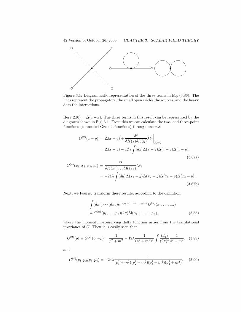
Figure 3.1: Diagrammatic representation of the three terms in Eq. (3.86). Thelines represent the propagators, the small open circles the sources, and the heavydots the interactions.

Here ∆(0) = ∆(x−x). The three terms in this result can be represented by thediagrams shown in Fig. 3.1. From this we can calculate the two- and three-pointfunctions (connected Green’s functions) through order λ:

G(2)(x − y) = ∆(x − y) +δ2

δK(x)δK(y)λδ1

∣

∣

∣

∣

K=0

= ∆(x − y) − 12λ

∫

(dz)∆(x − z)∆(z − z)∆(z − y),

(3.87a)

G(4)(x1, x2, x3, x4) =δ4

δK(x1) . . . δK(x4)λδ1

= −24λ

∫

(dy)∆(x1 − y)∆(x2 − y)∆(x3 − y)∆(x4 − y).

(3.87b)

Next, we Fourier transform these results, according to the definition:

∫

(dx1) · · · (dxn)e−ip1·x1−...−ipn·xnG(n)(x1, . . . , xn)

= G(n)(p1, . . . , pn)(2π)4δ(p1 + . . . + pn), (3.88)

where the momentum-conserving delta function arises from the translationalinvariance of G. Then it is easily seen that

G(2)(p) ≡ G(2)(p,−p) =1

p2 + m2− 12λ

1

(p2 + m2)2

∫

(dq)

(2π)41

q2 + m2, (3.89)

and

G(4)(p1, p2, p3, p4) = −24λ1

(p21 + m2)(p2

2 + m2)(p23 + m2)(p2

4 + m2). (3.90)

3.7. SECOND-ORDER PERTURBATION THEORY43 Version of October 26, 2009

3.7 Second-Order Perturbation Theory

Now let us proceed to second order in λ. The next term in δ, Eq. (3.84), is

λ2δ2[K] = e−W01

2

∫

(dx)λ

(

δ

δK(x)

)4 ∫

(dy)λ

(

δ

δK(y)

)4

eW0

= e−W01

2

∫

(dx)λ

(

δ

δK(x)

)4

eW0 (−λδ1[K]) , (3.91)

which uses Eq. (3.85). Next we use Leibnitz’ rule,

(

δ

δK(x)

)4

eW0δ1[K] =

[

(

δ

δK(x)

)4

eW0

]

δ1[K]

+ 4

[

(

δ

δK(x)

)3

eW0

]

δ

δK(x)δ1[K] + 6

[

(

δ

δK(x)

)2

eW0

]

(

δ

δK(x)

)2

δ1[K]

+ 4

[

δ

δK(x)eW0

](

δ

δK(x)

)3

δ1[K] + eW0

(

δ

δK(x)

)4

δ1[K]. (3.92)

We recognize in the first term here the square of the lowest order term:

δ2[K] =1

2(δ1[K])2 + δc

2[K], (3.93)

and so this first term cancels the δ21 term in the expansion of the logarithm in

W , Eq. (3.83):

W [K] = W0[K] + λδ1[K] − λ2

2(δ1[K])2 + λ2δ2[K] + . . . . (3.94)

We call δc2[K] the “connected part.” Referring to Eq. (3.86) we now easily work

it out:

δc2[K] =

1

2

∫

(dx)

{

4

[∫

(dy)(dz)(dw)∆(x − y)K(y)∆(x − z)K(z)

×∆(x − w)K(w) + 3∆(0)

∫

(dy)∆(x − y)K(y)

]

×[

4

∫

(dy)(dz)(dw)(du)∆(u − x)∆(u − y)∆(u − z)∆(u − w)

×K(y)K(z)K(w) + 12∆(0)

∫

(du)(dy)∆(u − x)∆(u − y)K(y)

]

+ 6

[∫

(dy)(dz)∆(x − y)∆(x − z)K(y)K(z) + ∆(0)

]

×[

12

∫

(du)(dy)(dz)∆(u − x)∆(u − x)∆(u − y)∆(u − z)K(y)K(z)


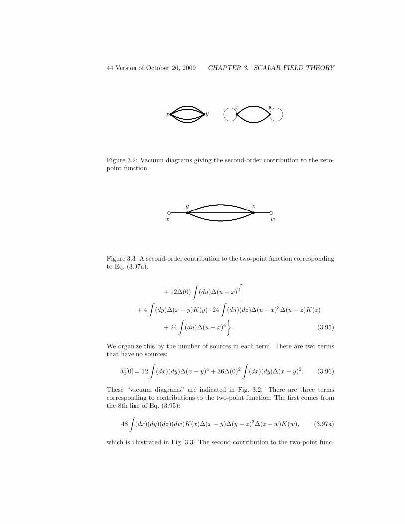
• •x y • •�� x y

Figure 3.2: Vacuum diagrams giving the second-order contribution to the zero-point function.

• •d dx w

y z

Figure 3.3: A second-order contribution to the two-point function correspondingto Eq. (3.97a).

+ 12∆(0)

∫

(du)∆(u − x)2]

+ 4

∫

(dy)∆(x − y)K(y) · 24

∫

(du)(dz)∆(u − x)3∆(u − z)K(z)

+ 24

∫

(du)∆(u − x)4}

. (3.95)

We organize this by the number of sources in each term. There are two termsthat have no sources:

δc2[0] = 12

∫

(dx)(dy)∆(x − y)4 + 36∆(0)2∫

(dx)(dy)∆(x − y)2. (3.96)

These “vacuum diagrams” are indicated in Fig. 3.2. There are three termscorresponding to contributions to the two-point function: The first comes fromthe 8th line of Eq. (3.95):

48

∫

(dx)(dy)(dz)(dw)K(x)∆(x − y)∆(y − z)3∆(z − w)K(w), (3.97a)

which is illustrated in Fig. 3.3. The second contribution to the two-point func-


•

•

d d��

x wy

z

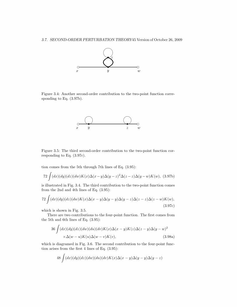
Figure 3.4: Another second-order contribution to the two-point function corre-sponding to Eq. (3.97b).

• •d d�� x wy z

Figure 3.5: The third second-order contribution to the two-point function cor-responding to Eq. (3.97c).

tion comes from the 5th through 7th lines of Eq. (3.95):

72

∫

(dx)(dy)(dz)(dw)K(x)∆(x− y)∆(y − z)2∆(z − z)∆(y−w)K(w), (3.97b)

is illustrated in Fig. 3.4. The third contribution to the two-point function comesfrom the 2nd and 4th lines of Eq. (3.95):

72

∫

(dx)(dy)(dz)(dw)K(x)∆(x − y)∆(y − y)∆(y − z)∆(z − z)∆(z − w)K(w),

(3.97c)which is shown in Fig. 3.5.

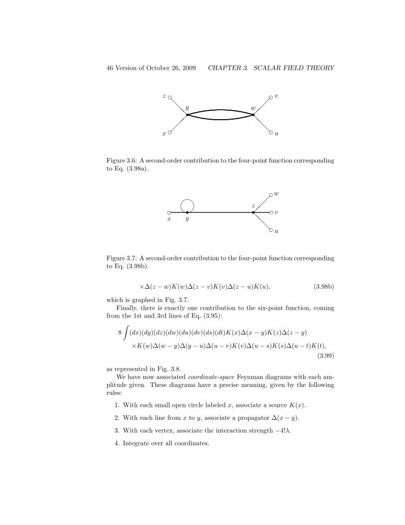
There are two contributions to the four-point function. The first comes fromthe 5th and 6th lines of Eq. (3.95):

36

∫

(dx)(dy)(dz)(dw)(du)(dv)K(x)∆(x − y)K(z)∆(z − y)∆(y − w)2

×∆(w − u)K(u)∆(w − v)K(v), (3.98a)

which is diagramed in Fig. 3.6. The second contribution to the four-point func-tion arises from the first 4 lines of Eq. (3.95):

48

∫

(dx)(dy)(dz)(dw)(du)(dv)K(x)∆(x − y)∆(y − y)∆(y − z)


• •

��

@@@

@@@

��

d

d

d

d

x

z

u

v

wy

Figure 3.6: A second-order contribution to the four-point function correspondingto Eq. (3.98a).

• •

@@@

��d d

d

dx

z

u

v

w

y

Figure 3.7: A second-order contribution to the four-point function correspondingto Eq. (3.98b).

×∆(z − w)K(w)∆(z − v)K(v)∆(z − u)K(u), (3.98b)

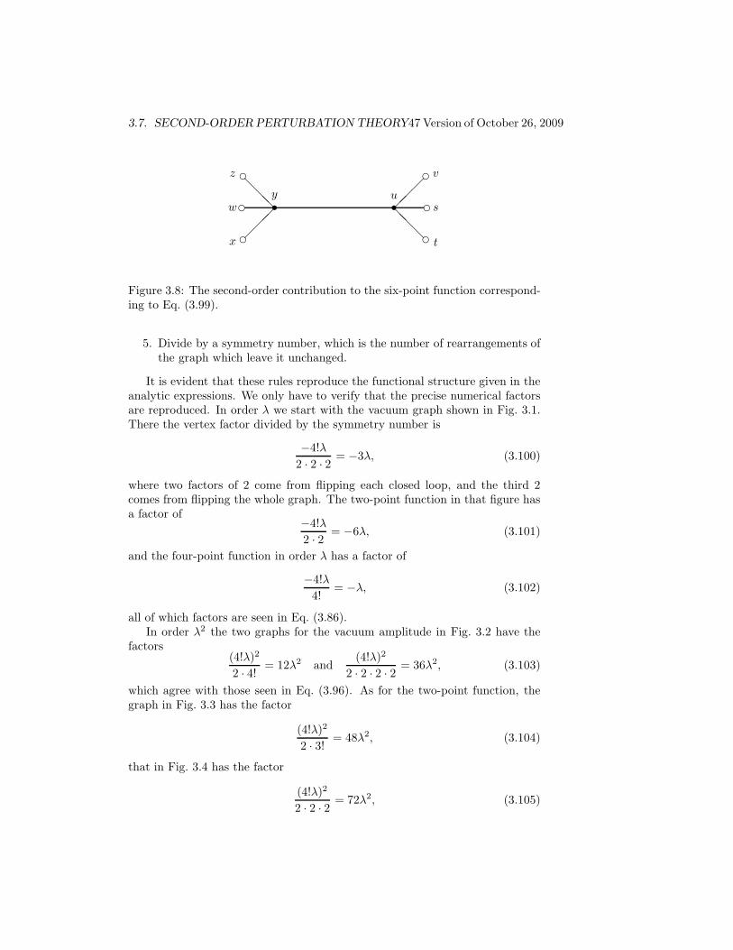
which is graphed in Fig. 3.7.Finally, there is exactly one contribution to the six-point function, coming

from the 1st and 3rd lines of Eq. (3.95):

8

∫

(dx)(dy)(dz)(dw)(du)(dv)(ds)(dt)K(x)∆(x − y)K(z)∆(z − y)

×K(w)∆(w − y)∆(y − u)∆(u − v)K(v)∆(u − s)K(s)∆(u − t)K(t),

(3.99)

as represented in Fig. 3.8.We have now associated coordinate-space Feynman diagrams with each am-

plitude given. These diagrams have a precise meaning, given by the followingrules:

1. With each small open circle labeled x, associate a source K(x).

2. With each line from x to y, associate a propagator ∆(x − y).

3. With each vertex, associate the interaction strength −4!λ.

4. Integrate over all coordinates.


• •

��

@@@

@@@

��

d

dd

d

dd

x

z

w

t

v

suy

Figure 3.8: The second-order contribution to the six-point function correspond-ing to Eq. (3.99).

5. Divide by a symmetry number, which is the number of rearrangements ofthe graph which leave it unchanged.

It is evident that these rules reproduce the functional structure given in theanalytic expressions. We only have to verify that the precise numerical factorsare reproduced. In order λ we start with the vacuum graph shown in Fig. 3.1.There the vertex factor divided by the symmetry number is

−4!λ

2 · 2 · 2 = −3λ, (3.100)

where two factors of 2 come from flipping each closed loop, and the third 2comes from flipping the whole graph. The two-point function in that figure hasa factor of

−4!λ

2 · 2 = −6λ, (3.101)

and the four-point function in order λ has a factor of

−4!λ

4!= −λ, (3.102)

all of which factors are seen in Eq. (3.86).In order λ2 the two graphs for the vacuum amplitude in Fig. 3.2 have the

factors(4!λ)2

2 · 4!= 12λ2 and

(4!λ)2

2 · 2 · 2 · 2 = 36λ2, (3.103)

which agree with those seen in Eq. (3.96). As for the two-point function, thegraph in Fig. 3.3 has the factor

(4!λ)2

2 · 3!= 48λ2, (3.104)

that in Fig. 3.4 has the factor

(4!λ)2

2 · 2 · 2 = 72λ2, (3.105)


and that in Fig. 3.5 has(4!λ)2

2 · 2 · 2 = 72λ2, (3.106)

coinciding with the amplitudes given in Eqs. (3.97a), (3.97b), and (3.97c), re-spectively. The four-point functions in Figs. 3.6 and 3.7 have the factors

(4!λ)2

2 · 2 · 2 · 2 = 36λ2 and(4!λ)2

2 · 3!= 48λ2, (3.107)

respectively, coinciding to what we had in Eqs. (3.98a) and (3.98b). Finally, thesix-point function in Fig. 3.8 has the factor

(4!λ)2

(3!)22= 8λ2, (3.108)

which agrees with Eq. (3.99).From these results we can easily obtain the Green’s functions through order

λ2. For example, from Eqs. (3.87a), (3.97a), (3.97b), and (3.97c), the two-pointfunction is

G(2)(x, y) = ∆(x − y) − 12λ

∫

(dz)∆(x − z)∆(z − z)∆(z − y)

+ 96λ2

∫

(dz)(dw)∆(x − z)∆(z − w)3∆(w − y)

+ 144λ2

∫

(dz)(dw)∆(x − z)∆(z − w)2∆(w − w)∆(z − y)

+ 144λ2

∫

(dz)(dw)∆(x − z)∆(z − z)∆(z − w)∆(w − w)

×∆(w − y) + O(λ3). (3.109)

By Fourier-transforming, as in Eq. (3.88), we find immediately

G(2)(p) =1

p2 + m2− 12λ

(p2 + m2)2

∫

(dl)

(2π)21

l2 + m2

+96λ2

(p2 + m2)2

∫

(dq1)

(2π)4(dq2)

(2π)4(dq3)

(2π)4(2π)4δ(q1 + q2 + q3 − p)

(q21 + m2)(q2

2 + m2)(q23 + m2)

+144λ2

(p2 + m2)2

∫

(dq1)

(2π)4(dq2)

(2π)4(2π)4δ(q1 + q2)

(q21 + m2)(q2

2 + m2)

∫

(dl)

(2π)41

l2 + m2

+144λ2

(p2 + m2)3

∫

(dl)

(2π)41

l2 + m2

∫

(dl′)

(2π)41

l′2 + m2+ O(λ3).

(3.110)

We represent these momentum-space Green’s functions by Feynman diagramsor graphs, where a line carrying momentum p is represented by 1/(p2 + m2),and a vertex corresponds to the factor −4!λ. To obtain G(n) to order λk, drawall topologically distinct graphs with n external lines having up to k four-point

3.8. MASS OPERATOR 49 Version of October 26, 2009

G(2)(p) = + •��+ • •

+ •

•��+ • •��

+ O(λ3)

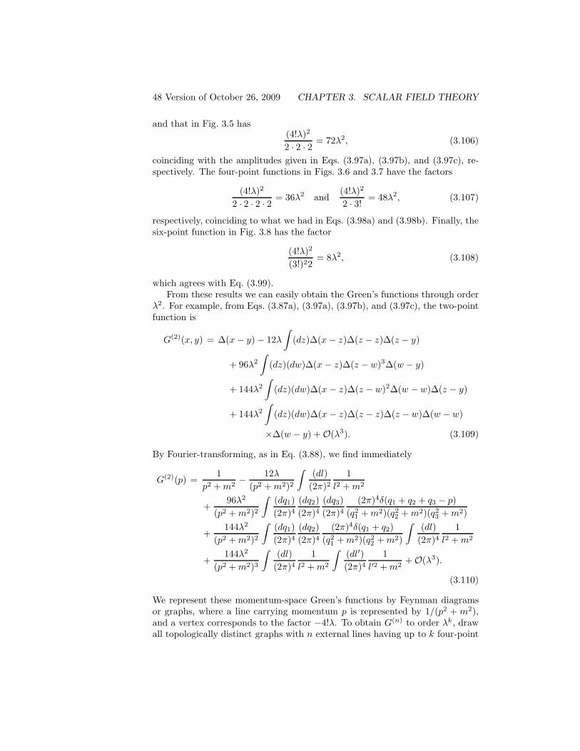
Figure 3.9: Feynman diagrams corresponding to the two-point Green’s function.

vertices. Conserve momentum at a vertex joining lines carrying momenta p1,p2, p3, p4 by supplying the factor (2π)4δ(p1 + p2 + p3 + p4), where we adoptthe convention that all momenta are flowing into the vertex. Integrate over allloop momentum, with the four-dimensional element (dl)/(2π)4. Divide by thesymmetry number.

We illustrate these rules for the two-point function, or modified propagationfunction, G(2), in Fig. 3.9. It is evident that the above rules reproduce theresults given in Eq. (3.110),where the symmetry numbers of the five graphsshown are 1, 2, 3!, 4, and 4, respectively, since the external lines carry a definitesense of momentum and therefore cannot be reversed.

It is convenient to introduce some further definitions.

• An amputated or truncated Green’s function has the propagators on theexternal legs removed. Thus, in order λ the amputated two-point functionis

−12λ

∫

(dl)

(2π)41

l2 + m2. (3.111)

• A one-particle irreducible or proper Green’s function is an amputatedGreen’s function which remains connected when any one internal line iscut. Thus, the first two O(λ2) contributions to G(2) in Fig. 3.9 are one-particle irreducible, while the third is not.

3.8 Mass Operator

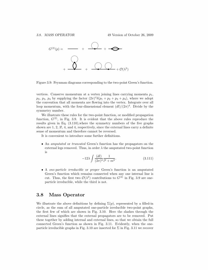
We illustrate the above definitions by defining Σ(p), represented by a filled-incircle, as the sum of all amputated one-particle irreducible two-point graphs,the first few of which are shown in Fig. 3.10. Here the slashes through theexternal lines signifies that the external propagators are to be removed. Putthese together by adding internal and external lines, so that we obtain the fullconnected Green’s function as shown in Fig. 3.11. Evidently, when the one-particle irreducible graphs in Fig. 3.10 are inserted for Σ in Fig. 3.11 we recover


/ ~ / = // •��+ / /• • + / /•

•��+ O(λ3)

Figure 3.10: Mass operator Σ(p) contributions through order λ2.

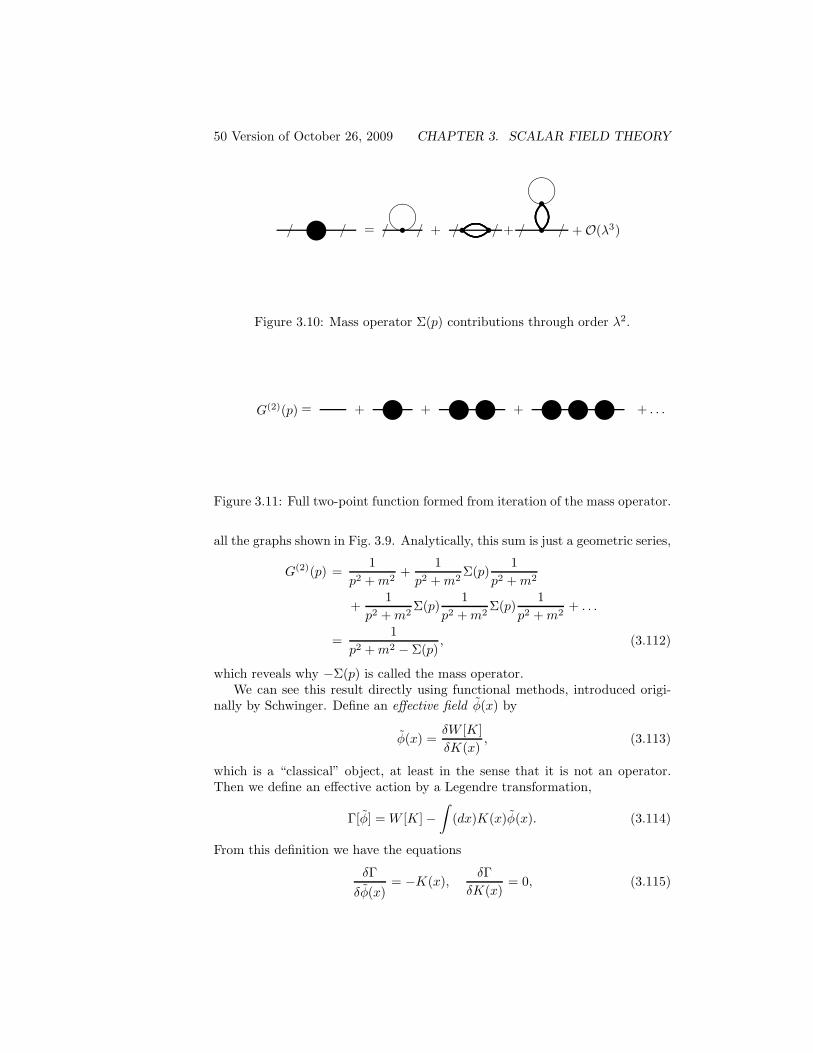
G(2)(p) = + ~ + ~ ~ + ~ ~ ~ + . . .

Figure 3.11: Full two-point function formed from iteration of the mass operator.

all the graphs shown in Fig. 3.9. Analytically, this sum is just a geometric series,

G(2)(p) =1

p2 + m2+

1

p2 + m2Σ(p)

1

p2 + m2

+1

p2 + m2Σ(p)

1

p2 + m2Σ(p)

1

p2 + m2+ . . .

=1

p2 + m2 − Σ(p), (3.112)

which reveals why −Σ(p) is called the mass operator.We can see this result directly using functional methods, introduced origi-

nally by Schwinger. Define an effective field φ̃(x) by

φ̃(x) =δW [K]

δK(x), (3.113)

which is a “classical” object, at least in the sense that it is not an operator.Then we define an effective action by a Legendre transformation,

Γ[φ̃] = W [K] −∫

(dx)K(x)φ̃(x). (3.114)

From this definition we have the equations

δΓ

δφ̃(x)= −K(x),

δΓ

δK(x)= 0, (3.115)

3.8. MASS OPERATOR 51 Version of October 26, 2009

so the implicit φ̃ dependence drops out. The one-particle irreducible graphs(Green’s functions) are defined by variations of the effective action with respectto the effective field:

Γ(n)(x1, . . . , xn) =δn

δφ̃(x1) . . . δφ̃(xn)Γ[φ̃]

∣

∣

∣

∣

φ̃=0

. (3.116)

For example, the irreducible two-point function is

Γ(2)(x, y) =δ2Γ

δφ̃(x)δφ̃(y)

∣

∣

∣

∣

φ̃=0

= −δK(x)

δφ̃(y)

∣

∣

∣

∣

φ̃=0

, (3.117)

while the corresponding connected Green’s function is

G(2)(x, y) =δ2W

δK(x)δK(y)

∣

∣

∣

∣

K=0

=δφ̃(y)

δK(x)

∣

∣

∣

∣

K=0

, (3.118)

which says that the two functions are inverses of each other,

G(2)−1 = −Γ(2), (3.119)

which is to be interpreted in the matrix sense, or∫

(dy)Γ(2)(x, y)G(2)(y, z) = −δ(x − z). (3.120)

In momentum space, this says

Γ(2)(p)G(2)(p) = −1, (3.121)

so according to Eq. (3.112),

Γ(2)(p) = −p2 − m2 + Σ(p), (3.122)

in which we see the expected appearance of the mass operator.It is worth recalling that for a free theory

W0[K] =1

2

∫

(dp)

(2π)4K(−p)

1

p2 + m2K(p), (3.123)

so then the effective field is

φ̃(p) =1

p2 + m2K(p), (3.124)

and so, substituting this into Eq. (3.114), we see that the effective action is

Γ0[φ̃] = −1

2

∫

(dp)

(2π)4φ̃(−p)(p2 + m2)φ̃(p), (3.125)

and thus the free one-particle irreducible two-point function is

Γ(2)0 (p) = −(p2 + m2), (3.126)

as seen in Eq. (3.122).

Scalar Field Theory - University of Oklahoma Physics ...milton/p6433/chap3.pdf · SCALAR FIELD...

Documents

Transcript of Scalar Field Theory - University of Oklahoma Physics ...milton/p6433/chap3.pdf · SCALAR FIELD...