Scalable Gaussian Processeszhenwendai.github.io/slides/gpss2018_slides.pdf · 2020-03-19 · Model...
57
Scalable Gaussian Processes Zhenwen Dai Amazon September 4, 2018 @GPSS2018 Zhenwen Dai (Amazon) Scalable Gaussian Processes September 4, 2018 @GPSS2018 1 / 55
Transcript of Scalable Gaussian Processeszhenwendai.github.io/slides/gpss2018_slides.pdf · 2020-03-19 · Model...
Scalable Gaussian Processes
Zhenwen Dai
Amazon
September 4, 2018 @GPSS2018
Zhenwen Dai (Amazon) Scalable Gaussian Processes September 4, 2018 @GPSS2018 1 / 55
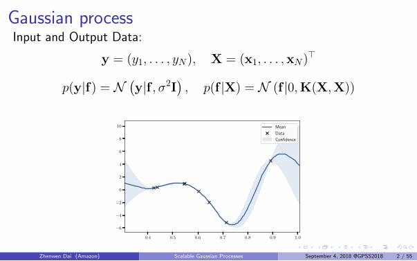
Gaussian processInput and Output Data:
y = (y1, . . . , yN), X = (x1, . . . ,xN)>
p(y|f) = N(y|f , σ2I
), p(f |X) = N (f |0,K(X,X))
0.4 0.5 0.6 0.7 0.8 0.9 1.0
−6
−4
−2
0
2
4
6
8
10 Mean
Data
Confidence
Zhenwen Dai (Amazon) Scalable Gaussian Processes September 4, 2018 @GPSS2018 2 / 55
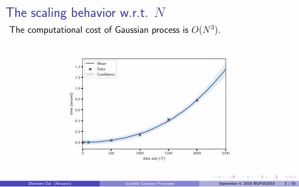
The scaling behavior w.r.t. NThe computational cost of Gaussian process is O(N 3).
0 500 1000 1500 2000 2500
data size (N)
0.0
0.2
0.4
0.6
0.8
1.0
1.2
1.4ti
me
(sec
ond
)
Mean
Data
Confidence
Zhenwen Dai (Amazon) Scalable Gaussian Processes September 4, 2018 @GPSS2018 3 / 55
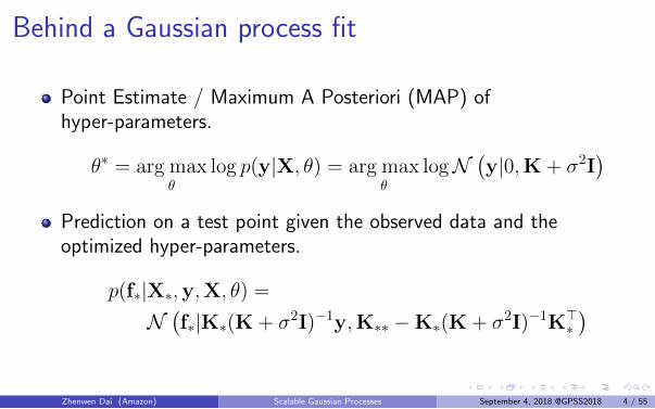
Behind a Gaussian process fit
Point Estimate / Maximum A Posteriori (MAP) ofhyper-parameters.
θ∗ = arg maxθ
log p(y|X, θ) = arg maxθ
logN(y|0,K + σ2I
)Prediction on a test point given the observed data and theoptimized hyper-parameters.
p(f∗|X∗,y,X, θ) =
N(f∗|K∗(K + σ2I)−1y,K∗∗ −K∗(K + σ2I)−1K>∗
)Zhenwen Dai (Amazon) Scalable Gaussian Processes September 4, 2018 @GPSS2018 4 / 55
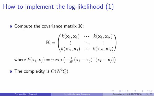
How to implement the log-likelihood (1)
Compute the covariance matrix K:
K =
k(x1,x1) · · · k(x1,xN)... . . . ...
k(xN ,x1) · · · k(xN ,xN)
where k(xi,xj) = γ exp
(− 1
2l2 (xi − xj)>(xi − xj)
)The complexity is O(N 2Q).
Zhenwen Dai (Amazon) Scalable Gaussian Processes September 4, 2018 @GPSS2018 5 / 55
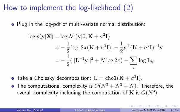
How to implement the log-likelihood (2)
Plug in the log-pdf of multi-variate normal distribution:
log p(y|X) = logN(y|0,K + σ2I
)=− 1
2log |2π(K + σ2I)| − 1
2y>(K + σ2I)−1y
=− 1
2(||L−1y||2 +N log 2π)−
∑i
log Lii
Take a Cholesky decomposition: L = chol(K + σ2I).
The computational complexity is O(N 3 +N 2 +N). Therefore, theoverall complexity including the computation of K is O(N 3).
Zhenwen Dai (Amazon) Scalable Gaussian Processes September 4, 2018 @GPSS2018 6 / 55
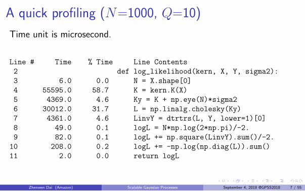
A quick profiling (N=1000, Q=10)
Time unit is microsecond.
Line # Time % Time Line Contents
2 def log_likelihood(kern, X, Y, sigma2):
3 6.0 0.0 N = X.shape[0]
4 55595.0 58.7 K = kern.K(X)
5 4369.0 4.6 Ky = K + np.eye(N)*sigma2
6 30012.0 31.7 L = np.linalg.cholesky(Ky)
7 4361.0 4.6 LinvY = dtrtrs(L, Y, lower=1)[0]
8 49.0 0.1 logL = N*np.log(2*np.pi)/-2.
9 82.0 0.1 logL += np.square(LinvY).sum()/-2.
10 208.0 0.2 logL += -np.log(np.diag(L)).sum()
11 2.0 0.0 return logL
Zhenwen Dai (Amazon) Scalable Gaussian Processes September 4, 2018 @GPSS2018 7 / 55
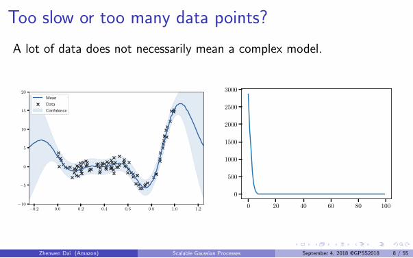
Too slow or too many data points?
A lot of data does not necessarily mean a complex model.
−0.2 0.0 0.2 0.4 0.6 0.8 1.0 1.2−10
−5
0
5
10
15
20
Mean
Data
Confidence
0 20 40 60 80 100
0
500
1000
1500
2000
2500
3000
Zhenwen Dai (Amazon) Scalable Gaussian Processes September 4, 2018 @GPSS2018 8 / 55
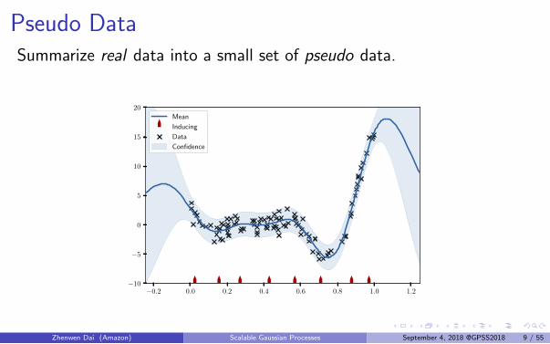
Pseudo DataSummarize real data into a small set of pseudo data.
−0.2 0.0 0.2 0.4 0.6 0.8 1.0 1.2−10
−5
0
5
10
15
20
Mean
Inducing
Data
Confidence
Zhenwen Dai (Amazon) Scalable Gaussian Processes September 4, 2018 @GPSS2018 9 / 55
Sparse Gaussian Process
Sparse GPs refers to a family of approximations:
Nystrom approximation [Williams and Seeger, 2001]
Fully independent training conditional (FITC) [Snelson andGhahramani, 2006]
Variational sparse Gaussian process [Titsias, 2009]
Zhenwen Dai (Amazon) Scalable Gaussian Processes September 4, 2018 @GPSS2018 10 / 55
Approximation by subset
Let’s randomly pick a subset from the training data: Z ∈ RM×Q.
Approximate the covariance matrix K by K.
K = KzK−1zz K>z , where Kz = K(X,Z) and Kzz = K(Z,Z).
Note that K ∈ RN×N , Kz ∈ RN×M and Kzz ∈ RM×M .
The log-likelihood is approximated by
log p(y|X, θ) ≈ logN(y|0,KzK
−1zz K>z + σ2I
).
Zhenwen Dai (Amazon) Scalable Gaussian Processes September 4, 2018 @GPSS2018 11 / 55
Efficient computation using Woodbury formula
The naive formulation does not bring any computational benefits.
L = −1
2log |2π(K + σ2I)| − 1
2y>(K + σ2I)−1y
Apply the Woodbury formula:
(KzK−1zz K>z + σ2I)−1 = σ−2I− σ−4Kz(Kzz + σ−2K>z Kz)
−1K>z
Note that (Kzz + σ−2K>z Kz) ∈ RM×M .
The computational complexity reduces to O(NM 2).
Zhenwen Dai (Amazon) Scalable Gaussian Processes September 4, 2018 @GPSS2018 12 / 55
Nystrom approximation
The above approach is called Nystrom approximation by Williamsand Seeger [2001].
The approximation is directly done on the covariance matrixwithout the concept of pseudo data.
The approximation becomes exact if the whole data set is taken,i.e., KK−1K> = K.
The subset selection is done randomly.
Zhenwen Dai (Amazon) Scalable Gaussian Processes September 4, 2018 @GPSS2018 13 / 55
Gaussian process with Pseudo Data (1)
Snelson and Ghahramani [2006] proposes the idea of having pseudodata. This approach is later referred to as Fully independenttraining conditional (FITC).
Augment the training data (X, y) with pseudo data u at locationZ.
p
([yu
]|[XZ
])=N
([yu
]|0,[Kff + σ2I Kfu
K>fu Kuu
])where Kff = K(X,X), Kfu = K(X,Z) and Kuu = K(Z,Z).
Zhenwen Dai (Amazon) Scalable Gaussian Processes September 4, 2018 @GPSS2018 14 / 55
Gaussian process with Pseudo Data (2)
Thanks to the marginalization property of Gaussian distribution,
p(y|X) =
∫u
p(y,u|X,Z).
Further re-arrange the notation:
p(y,u|X,Z) = p(y|u,X,Z)p(u|Z)
where p(u|Z) = N (u|0,Kuu),p(y|u,X,Z) = N
(y|KfuK
−1uuu,Kff −KfuK
−1uuK>fu + σ2I
).
Zhenwen Dai (Amazon) Scalable Gaussian Processes September 4, 2018 @GPSS2018 15 / 55
FITC approximation (1)
So far, p(y|X) has not been changed, but there is no speed-up,Kff ∈ RN×N in Kff −KfuK
−1uuK>fu + σ2I.
The FITC approximation assumes
p(y|u,X,Z) = N(y|KfuK
−1uuu,Λ + σ2I
),
where Λ = (Kff −KfuK−1uuK>fu) ◦ I.
Zhenwen Dai (Amazon) Scalable Gaussian Processes September 4, 2018 @GPSS2018 16 / 55
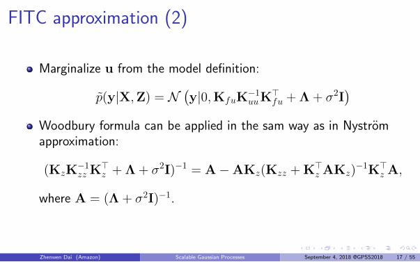
FITC approximation (2)
Marginalize u from the model definition:
p(y|X,Z) = N(y|0,KfuK
−1uuK>fu + Λ + σ2I
)Woodbury formula can be applied in the sam way as in Nystromapproximation:
(KzK−1zz K>z + Λ + σ2I)−1 = A−AKz(Kzz + K>z AKz)
−1K>z A,
where A = (Λ + σ2I)−1.
Zhenwen Dai (Amazon) Scalable Gaussian Processes September 4, 2018 @GPSS2018 17 / 55
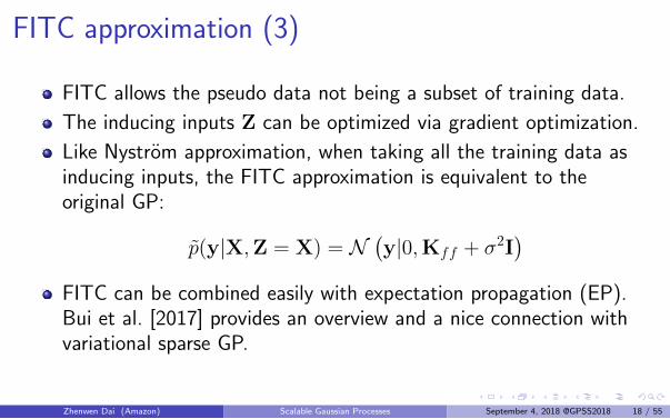
FITC approximation (3)
FITC allows the pseudo data not being a subset of training data.
The inducing inputs Z can be optimized via gradient optimization.
Like Nystrom approximation, when taking all the training data asinducing inputs, the FITC approximation is equivalent to theoriginal GP:
p(y|X,Z = X) = N(y|0,Kff + σ2I
)FITC can be combined easily with expectation propagation (EP).Bui et al. [2017] provides an overview and a nice connection withvariational sparse GP.
Zhenwen Dai (Amazon) Scalable Gaussian Processes September 4, 2018 @GPSS2018 18 / 55
Model Approximation vs. Approximate Inference
When the exact model/inference is intractable, typically there are twotypes of approaches:
Approximate the original model with a simpler one such thatinference becomes tractable, like Nystrom approximation, FITC.
Keep the original model but derive an approximate inferencemethod which is often not able to return the true answer, likevariational inference.
Zhenwen Dai (Amazon) Scalable Gaussian Processes September 4, 2018 @GPSS2018 19 / 55
Model Approximation vs. Approximate Inference
A problem with model approximation is that
when an approximated model requires some tuning, e.g., forhyper-parameters, it is unclear how to improve it based on trainingdata.
In the case of FITC, we know the model is correct if Z = X,however, optimizing Z will not necessarily lead to a better location.
In fact, optimizing Z can lead to overfitting. [Quinonero-Candelaand Rasmussen, 2005]
Zhenwen Dai (Amazon) Scalable Gaussian Processes September 4, 2018 @GPSS2018 20 / 55
Variational Sparse Gaussian Process (1)
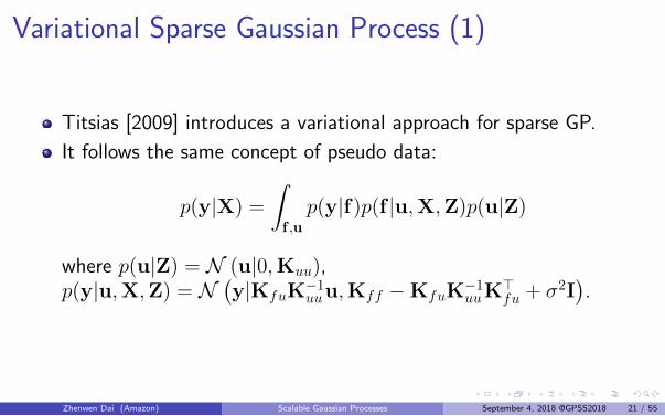
Titsias [2009] introduces a variational approach for sparse GP.
It follows the same concept of pseudo data:
p(y|X) =
∫f ,u
p(y|f)p(f |u,X,Z)p(u|Z)
where p(u|Z) = N (u|0,Kuu),p(y|u,X,Z) = N
(y|KfuK
−1uuu,Kff −KfuK
−1uuK>fu + σ2I
).
Zhenwen Dai (Amazon) Scalable Gaussian Processes September 4, 2018 @GPSS2018 21 / 55
Variational Sparse Gaussian Process (2)
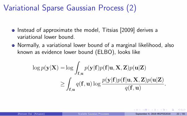
Instead of approximate the model, Titsias [2009] derives avariational lower bound.
Normally, a variational lower bound of a marginal likelihood, alsoknown as evidence lower bound (ELBO), looks like
log p(y|X) = log
∫f ,u
p(y|f)p(f |u,X,Z)p(u|Z)
≥∫f ,u
q(f ,u) logp(y|f)p(f |u,X,Z)p(u|Z)
q(f ,u).
Zhenwen Dai (Amazon) Scalable Gaussian Processes September 4, 2018 @GPSS2018 22 / 55
Special Variational Posterior
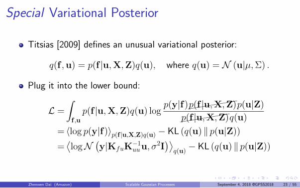
Titsias [2009] defines an unusual variational posterior:
q(f ,u) = p(f |u,X,Z)q(u), where q(u) = N (u|µ,Σ) .
Plug it into the lower bound:
L =
∫f ,u
p(f |u,X,Z)q(u) logp(y|f)(((((
(((p(f |u,X,Z)p(u|Z)
(((((((
(p(f |u,X,Z)q(u)
= 〈log p(y|f)〉p(f |u,X,Z)q(u) − KL (q(u) ‖ p(u|Z))
=⟨logN
(y|KfuK
−1uuu, σ2I
)⟩q(u)− KL (q(u) ‖ p(u|Z))
Zhenwen Dai (Amazon) Scalable Gaussian Processes September 4, 2018 @GPSS2018 23 / 55
Special Variational Posterior
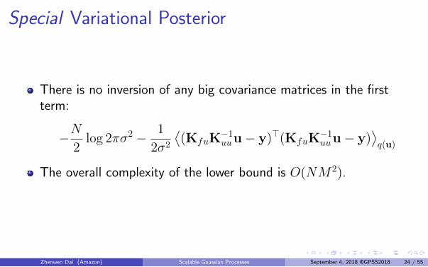
There is no inversion of any big covariance matrices in the firstterm:
−N2
log 2πσ2 − 1
2σ2
⟨(KfuK
−1uuu− y)>(KfuK
−1uuu− y)
⟩q(u)
The overall complexity of the lower bound is O(NM 2).
Zhenwen Dai (Amazon) Scalable Gaussian Processes September 4, 2018 @GPSS2018 24 / 55
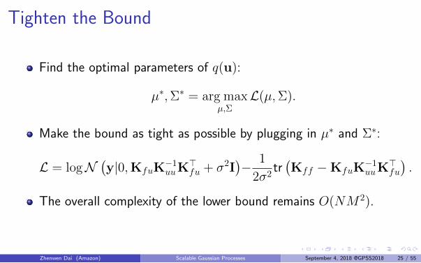
Tighten the Bound
Find the optimal parameters of q(u):
µ∗,Σ∗ = arg maxµ,Σ
L(µ,Σ).
Make the bound as tight as possible by plugging in µ∗ and Σ∗:
L = logN(y|0,KfuK
−1uuK>fu + σ2I
)− 1
2σ2tr(Kff −KfuK
−1uuK>fu
).
The overall complexity of the lower bound remains O(NM 2).
Zhenwen Dai (Amazon) Scalable Gaussian Processes September 4, 2018 @GPSS2018 25 / 55
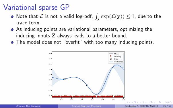
Variational sparse GPNote that L is not a valid log-pdf,
∫y exp(L(y)) ≤ 1, due to the
trace term.As inducing points are variational parameters, optimizing theinducing inputs Z always leads to a better bound.The model does not “overfit” with too many inducing points.
0.4 0.5 0.6 0.7 0.8 0.9 1.0
−6
−4
−2
0
2
4
6
8
10 Mean
Inducing
Data
Confidence
Zhenwen Dai (Amazon) Scalable Gaussian Processes September 4, 2018 @GPSS2018 26 / 55
An alternative view of sparse GP
Is variational sparse GP a hack only working for GP?
Zhenwen Dai (Amazon) Scalable Gaussian Processes September 4, 2018 @GPSS2018 27 / 55
The two key ingredients
The two key ingredients of variational sparse GP:
Variational compression [Hensman and Lawrence, 2014]
Variational posterior with “pseudo data” (“variational Gaussianprocess” by Tran et al. [2016])
Zhenwen Dai (Amazon) Scalable Gaussian Processes September 4, 2018 @GPSS2018 28 / 55
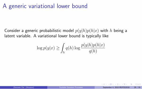
A generic variational lower bound
Consider a generic probabilistic model p(y|h)p(h|x) with h being alatent variable. A variational lower bound is typically like
log p(y|x) ≥∫h
q(h) logp(y|h)p(h|x)
q(h)
Zhenwen Dai (Amazon) Scalable Gaussian Processes September 4, 2018 @GPSS2018 29 / 55
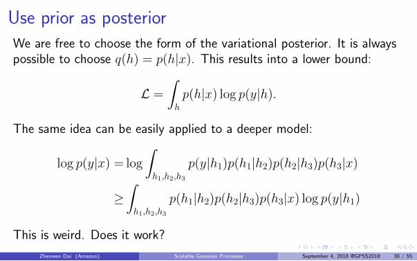
Use prior as posteriorWe are free to choose the form of the variational posterior. It is alwayspossible to choose q(h) = p(h|x). This results into a lower bound:
L =
∫h
p(h|x) log p(y|h).
The same idea can be easily applied to a deeper model:
log p(y|x) = log
∫h1,h2,h3
p(y|h1)p(h1|h2)p(h2|h3)p(h3|x)
≥∫h1,h2,h3
p(h1|h2)p(h2|h3)p(h3|x) log p(y|h1)
This is weird. Does it work?
Zhenwen Dai (Amazon) Scalable Gaussian Processes September 4, 2018 @GPSS2018 30 / 55
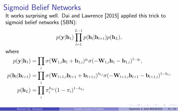
Sigmoid Belief NetworksIt works surprising well. Dai and Lawrence [2015] applied this trick tosigmoid belief networks (SBN):
p(y|h1)L−1∏l=1
p(hl|hl+1)p(hL),
where
p(y|h1) =∏i
σ(W1,ih1 + b1,i)yiσ(−W1,ih1 − b1,i)
1−yi,
p(hl|hl+1) =∏i
σ(Wl+1,ihl+1 + bl+1,i)hl,iσ(−Wl+1,ihl+1 − bl+1,i)
1−hl,i
p(hL) =∏i
πhLi
i (1− πi)1−hLi
L =
∫h1,...,hL
q(hL)L−1∏l=1
p(hl|hl+1) log p(y|h1)
Zhenwen Dai (Amazon) Scalable Gaussian Processes September 4, 2018 @GPSS2018 31 / 55
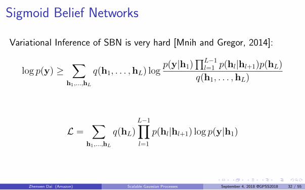
Sigmoid Belief Networks
Variational Inference of SBN is very hard [Mnih and Gregor, 2014]:
log p(y) ≥∑
h1,...,hL
q(h1, . . . ,hL) logp(y|h1)
∏L−1l=1 p(hl|hl+1)p(hL)
q(h1, . . . ,hL)
L =∑
h1,...,hL
q(hL)L−1∏l=1
p(hl|hl+1) log p(y|h1)
Zhenwen Dai (Amazon) Scalable Gaussian Processes September 4, 2018 @GPSS2018 32 / 55
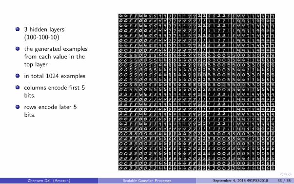
3 hidden layers(100-100-10)
the generated examplesfrom each value in thetop layer
in total 1024 examples
columns encode first 5bits.
rows encode later 5bits.
Zhenwen Dai (Amazon) Scalable Gaussian Processes September 4, 2018 @GPSS2018 33 / 55
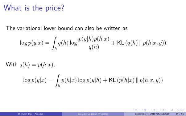
What is the price?
The variational lower bound can also be written as
log p(y|x) =
∫h
q(h) logp(y|h)p(h|x)
q(h)+ KL (q(h) ‖ p(h|x, y))
With q(h) = p(h|x),
log p(y|x) =
∫h
p(h|x) log p(y|h) + KL (p(h|x) ‖ p(h|x, y))
Zhenwen Dai (Amazon) Scalable Gaussian Processes September 4, 2018 @GPSS2018 34 / 55
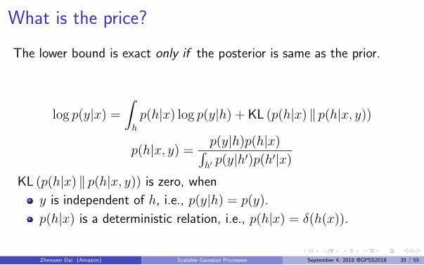
What is the price?
The lower bound is exact only if the posterior is same as the prior.
log p(y|x) =
∫h
p(h|x) log p(y|h) + KL (p(h|x) ‖ p(h|x, y))
p(h|x, y) =p(y|h)p(h|x)∫h′ p(y|h′)p(h′|x)
KL (p(h|x) ‖ p(h|x, y)) is zero, when
y is independent of h, i.e., p(y|h) = p(y).
p(h|x) is a deterministic relation, i.e., p(h|x) = δ(h(x)).
Zhenwen Dai (Amazon) Scalable Gaussian Processes September 4, 2018 @GPSS2018 35 / 55
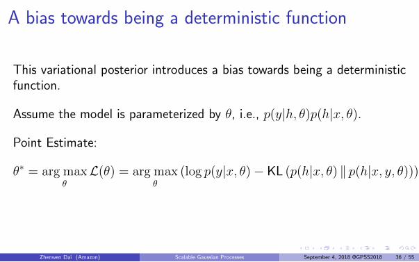
A bias towards being a deterministic function
This variational posterior introduces a bias towards being a deterministicfunction.
Assume the model is parameterized by θ, i.e., p(y|h, θ)p(h|x, θ).
Point Estimate:
θ∗ = arg maxθ
L(θ) = arg maxθ
(log p(y|x, θ)− KL (p(h|x, θ) ‖ p(h|x, y, θ)))
Zhenwen Dai (Amazon) Scalable Gaussian Processes September 4, 2018 @GPSS2018 36 / 55
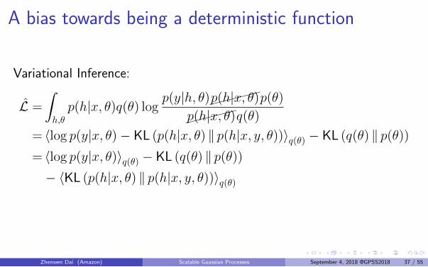
A bias towards being a deterministic function
Variational Inference:
L =
∫h,θ
p(h|x, θ)q(θ) logp(y|h, θ)������p(h|x, θ)p(θ)
������p(h|x, θ)q(θ)
= 〈log p(y|x, θ)− KL (p(h|x, θ) ‖ p(h|x, y, θ))〉q(θ) − KL (q(θ) ‖ p(θ))= 〈log p(y|x, θ)〉q(θ) − KL (q(θ) ‖ p(θ))− 〈KL (p(h|x, θ) ‖ p(h|x, y, θ))〉q(θ)
Zhenwen Dai (Amazon) Scalable Gaussian Processes September 4, 2018 @GPSS2018 37 / 55
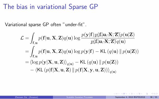
The bias in variational Sparse GP
Variational sparse GP often ”under-fit”.
L =
∫f ,u
p(f |u,X,Z)q(u) logp(y|f)(((((
(((p(f |u,X,Z)p(u|Z)
(((((((
(p(f |u,X,Z)q(u)
=
∫f ,u
p(f |u,X,Z)q(u) log p(y|f)− KL (q(u) ‖ p(u|Z))
= 〈log p(y|X,u,Z)〉q(u) − KL (q(u) ‖ p(u|Z))
− 〈KL (p(f |X,u,Z) ‖ p(f |X,y,u,Z))〉q(u)
Zhenwen Dai (Amazon) Scalable Gaussian Processes September 4, 2018 @GPSS2018 38 / 55
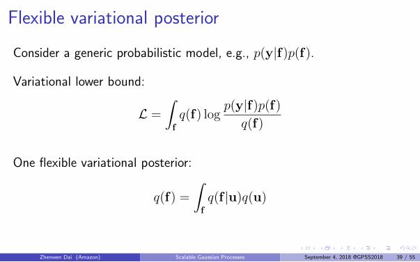
Flexible variational posterior
Consider a generic probabilistic model, e.g., p(y|f)p(f).
Variational lower bound:
L =
∫f
q(f) logp(y|f)p(f)
q(f)
One flexible variational posterior:
q(f) =
∫f
q(f |u)q(u)
Zhenwen Dai (Amazon) Scalable Gaussian Processes September 4, 2018 @GPSS2018 39 / 55
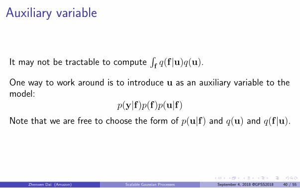
Auxiliary variable
It may not be tractable to compute∫f q(f |u)q(u).
One way to work around is to introduce u as an auxiliary variable to themodel:
p(y|f)p(f)p(u|f)
Note that we are free to choose the form of p(u|f) and q(u) and q(f |u).
Zhenwen Dai (Amazon) Scalable Gaussian Processes September 4, 2018 @GPSS2018 40 / 55
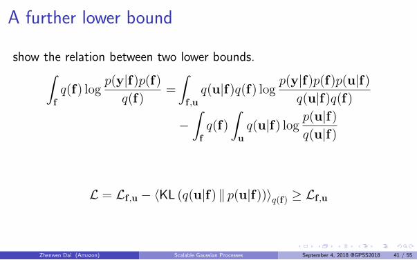
A further lower bound
show the relation between two lower bounds.∫f
q(f) logp(y|f)p(f)
q(f)=
∫f ,u
q(u|f)q(f) logp(y|f)p(f)p(u|f)
q(u|f)q(f)
−∫f
q(f)
∫u
q(u|f) logp(u|f)
q(u|f)
L = Lf ,u − 〈KL (q(u|f) ‖ p(u|f))〉q(f) ≥ Lf ,u
Zhenwen Dai (Amazon) Scalable Gaussian Processes September 4, 2018 @GPSS2018 41 / 55
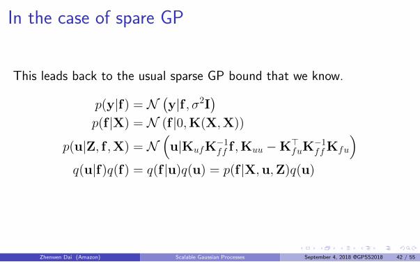
In the case of spare GP
This leads back to the usual sparse GP bound that we know.
p(y|f) = N(y|f , σ2I
)p(f |X) = N (f |0,K(X,X))
p(u|Z, f ,X) = N(u|KufK
−1ff f ,Kuu −K>fuK
−1ffKfu
)q(u|f)q(f) = q(f |u)q(u) = p(f |X,u,Z)q(u)
Zhenwen Dai (Amazon) Scalable Gaussian Processes September 4, 2018 @GPSS2018 42 / 55
Parallel Sparse Gaussian Process
Beyond Approximate the inference method, maybe we could exploitparallelization.
For Gaussian process, it turns out to be very hard, because parallelCholesky decomposition is very difficult.
Dai et al. [2014] and Gal et al. [2014] proposes a parallel inferencemethod for sparse GP.
Zhenwen Dai (Amazon) Scalable Gaussian Processes September 4, 2018 @GPSS2018 43 / 55
Data Parallelism
Consider a training set: D = {(x1, y1), . . . , (xN , yN)}.Assume there are C computational cores/machines.
A data parallelism algorithm divides the data set into C partitionsas evenly as possible: D =
⋃Cc=1Dc.
The parallelism happens in the way that the function running oneach core only requiring the data from the local partition.
Zhenwen Dai (Amazon) Scalable Gaussian Processes September 4, 2018 @GPSS2018 44 / 55
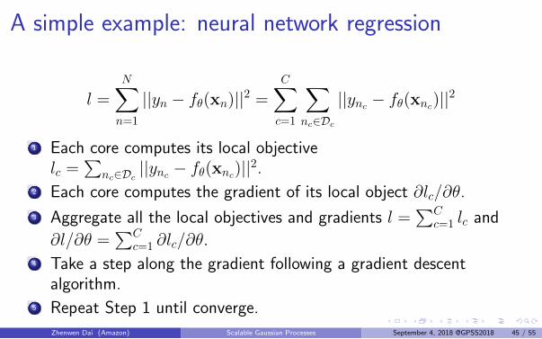
A simple example: neural network regression
l =N∑n=1
||yn − fθ(xn)||2 =C∑c=1
∑nc∈Dc
||ync − fθ(xnc)||2
1 Each core computes its local objectivelc =
∑nc∈Dc
||ync − fθ(xnc)||2.2 Each core computes the gradient of its local object ∂lc/∂θ.
3 Aggregate all the local objectives and gradients l =∑C
c=1 lc and
∂l/∂θ =∑C
c=1 ∂lc/∂θ.4 Take a step along the gradient following a gradient descent
algorithm.5 Repeat Step 1 until converge.
Zhenwen Dai (Amazon) Scalable Gaussian Processes September 4, 2018 @GPSS2018 45 / 55
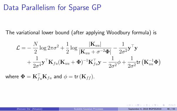
Data Parallelism for Sparse GP
The variational lower bound (after applying Woodbury formula) is
L =− N
2log 2πσ2 +
1
2log
|Kuu||Kuu + σ−2Φ| −
1
2σ2y>y
+1
2σ4y>Kfu(Kuu + Φ)−1K>fuy −
1
2σ2φ+
1
2σ2tr(K−1uuΦ
)where Φ = K>fuKfu and φ = tr (Kff).
Zhenwen Dai (Amazon) Scalable Gaussian Processes September 4, 2018 @GPSS2018 46 / 55
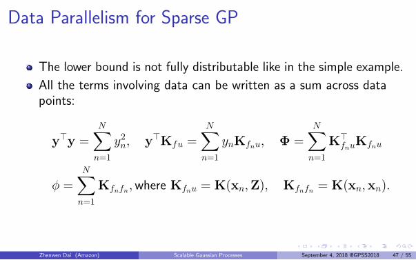
Data Parallelism for Sparse GP
The lower bound is not fully distributable like in the simple example.
All the terms involving data can be written as a sum across datapoints:
y>y =N∑n=1
y2n, y>Kfu =
N∑n=1
ynKfnu, Φ =N∑n=1
K>fnuKfnu
φ =N∑n=1
Kfnfn,where Kfnu = K(xn,Z), Kfnfn = K(xn,xn).
Zhenwen Dai (Amazon) Scalable Gaussian Processes September 4, 2018 @GPSS2018 47 / 55
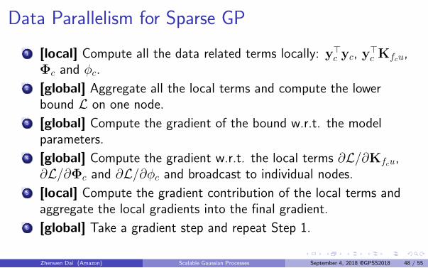
Data Parallelism for Sparse GP
1 [local] Compute all the data related terms locally: y>c yc, y>c Kfcu,Φc and φc.
2 [global] Aggregate all the local terms and compute the lowerbound L on one node.
3 [global] Compute the gradient of the bound w.r.t. the modelparameters.
4 [global] Compute the gradient w.r.t. the local terms ∂L/∂Kfcu,∂L/∂Φc and ∂L/∂φc and broadcast to individual nodes.
5 [local] Compute the gradient contribution of the local terms andaggregate the local gradients into the final gradient.
6 [global] Take a gradient step and repeat Step 1.
Zhenwen Dai (Amazon) Scalable Gaussian Processes September 4, 2018 @GPSS2018 48 / 55
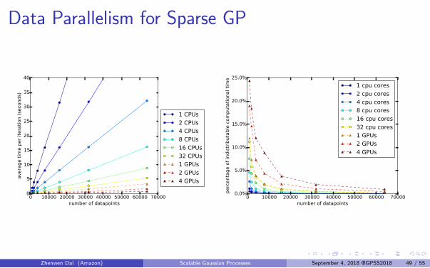
Data Parallelism for Sparse GP
0 10000 20000 30000 40000 50000 60000 70000number of datapoints
0
5
10
15
20
25
30
35
40
avera
ge t
ime p
er
itera
tion (
seco
nds)
1 CPUs
2 CPUs
4 CPUs
8 CPUs
16 CPUs
32 CPUs
1 GPUs
2 GPUs
4 GPUs
0 10000 20000 30000 40000 50000 60000 70000number of datapoints
0.0%
5.0%
10.0%
15.0%
20.0%
25.0%
perc
enta
ge o
f in
dis
trib
uta
ble
com
puta
tional ti
me
1 cpu cores
2 cpu cores
4 cpu cores
8 cpu cores
16 cpu cores
32 cpu cores
1 GPUs
2 GPUs
4 GPUs
Zhenwen Dai (Amazon) Scalable Gaussian Processes September 4, 2018 @GPSS2018 49 / 55
The emerge of deep learning platforms
Deep learning platforms such as Theano, Tensorflow, Torch, Caffe,MXNet emerge in recent years.
It standardizes deep neural networks programming.
Auto-differentiation enables the flexible construction of DNNs.
GPU acceleration enables scalability for real world applications.
Zhenwen Dai (Amazon) Scalable Gaussian Processes September 4, 2018 @GPSS2018 50 / 55
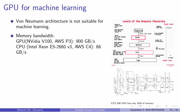
GPU for machine learning
Von Neumann architecture is not suitable formachine learning.
Memory bandwidth:GPU(NVidia V100, AWS P3): 900 GB/sCPU (Intel Xeon E5-2660 v3, AWS C4): 68GB/s
GTX 580 GPU has only 3GB of memory
Zhenwen Dai (Amazon) Scalable Gaussian Processes September 4, 2018 @GPSS2018 51 / 55
Probabilistic Programming on deep learning platforms
Edward http://edwardlib.org
PyMC3 https://github.com/pymc-devs/pymc3
pyprob https://github.com/probprog/pyprob
Pyro https://github.com/uber/pyro
Zhenwen Dai (Amazon) Scalable Gaussian Processes September 4, 2018 @GPSS2018 52 / 55
GP on deep learning platforms
GPflow https://github.com/GPflow/GPflow
GPyTorch https://github.com/cornellius-gp/gpytorch
Zhenwen Dai (Amazon) Scalable Gaussian Processes September 4, 2018 @GPSS2018 53 / 55
MXFusion and GPy2
Beyond GPU acceleration and auto-differentiation
Use Gaussian process as a building block.
MXFusion: modular probabilistic programming languagehttps://github.com/amzn/MXFusion
GPy2 (a new interface based on MXFusion):I writing new kernel with auto-differentiationI scalable inference on GPUI Construct hybrid GP, deep GP, recurrent GP by re-using GP module with
scalable approximate inference.
Zhenwen Dai (Amazon) Scalable Gaussian Processes September 4, 2018 @GPSS2018 54 / 55
Acknowledgement.
James’s blog: https://www.prowler.io/blog/
sparse-gps-approximate-the-posterior-not-the-model
Zhenwen Dai (Amazon) Scalable Gaussian Processes September 4, 2018 @GPSS2018 55 / 55
Thang D Bui, Josiah Yan, and Richard E Turner. A unifying framework for gaussian processpseudo-point approximations using power expectation propagation. Journal of Machine LearningResearch, 18:3649–3720, 2017.
Zhenwen Dai and Neil D. Lawrence. Variational hierarchical community of experts. In ICML DeepLearning workshop, 2015.
Zhenwen Dai, Andreas Damianou, James Hensman, and Neil D. Lawrence. Gaussian process modelswith parallelization and gpu acceleration. In NIPS workshop Software Engineering for MachineLearning, 2014.
Yarin Gal, Mark van der Wilk, and Carl Edward Rasmussen. Distributed variational inference in sparsegaussian process regression and latent variable models. In Advances in Neural InformationProcessing Systems 27, pages 3257–3265, 2014.
James Hensman and Neil D. Lawrence. Nested variational compression in deep gaussian processes.arXiv:1412.1370, 2014.
Andriy Mnih and Karol Gregor. Neural variational inference and learning in belief networks. InInternational Conference on Machine Learning, 2014.
Joaquin Quinonero-Candela and Carl Edward Rasmussen. A unifying view of sparse approximategaussian process regression. Journal of Machine Learning Research, 6:1939–1959, 2005.
Edward Snelson and Zoubin Ghahramani. Sparse gaussian processes using pseudo-inputs. In Advancesin Neural Information Processing Systems, pages 1257–1264. 2006.
Michalis Titsias. Variational learning of inducing variables in sparse gaussian processes. InProceedings of the Twelth International Conference on Artificial Intelligence and Statistics, pages567–574, 2009.
Zhenwen Dai (Amazon) Scalable Gaussian Processes September 4, 2018 @GPSS2018 55 / 55
Dustin Tran, Rajesh Ranganath, and David M. Blei. The variational gaussian process. In InternationalConference on Learning Representations, 2016.
Christopher K. I. Williams and Matthias Seeger. Using the nystrom method to speed up kernelmachines. In Advances in Neural Information Processing Systems, pages 682–688. 2001.
Zhenwen Dai (Amazon) Scalable Gaussian Processes September 4, 2018 @GPSS2018 55 / 55