155S8.5_3 Testing a Claim About a Mean: σ Not Known

1

April 03, 2012

Chapter 8Hypothesis Testing

8­1 Review and Preview8­2 Basics of Hypothesis Testing8­3 Testing a Claim about a Proportion8­4 Testing a Claim About a Mean: σ Known8­5 Testing a Claim About a Mean: σ Not Known8­6 Testing a Claim About a Standard Deviation or

Variance

MAT 155 Statistical AnalysisDr. Claude Moore

Cape Fear Community College

Key ConceptThis section presents methods for testing a claim about a population mean when we do not know the value of σ. The methods of this section use the Student t distribution introduced earlier. σ is unknown

Notationn = sample size= sample mean= population mean of all sample means from samples of size n

Requirements for Testing Claims About a Population

Mean (with σ Not Known)1) The sample is a simple random sample.2) The value of the population standard deviation σ is not known.3) Either or both of these conditions is satisfied:

The population is normally distributed or n > 30.

Test Statistic for Testing a Claim About a Mean (with σ Not Known)

P­values and Critical Values• Found in Table A­3• Degrees of freedom (df) = n – 1

155S8.5_3 Testing a Claim About a Mean: σ Not Known

2

April 03, 2012

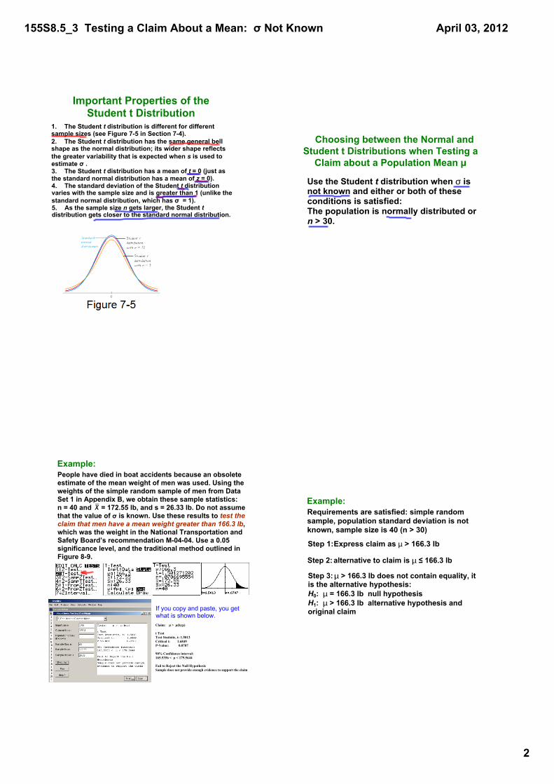
Important Properties of the Student t Distribution

1. The Student t distribution is different for different sample sizes (see Figure 7­5 in Section 7­4).2. The Student t distribution has the same general bell shape as the normal distribution; its wider shape reflects the greater variability that is expected when s is used to estimate σ .3. The Student t distribution has a mean of t = 0 (just as the standard normal distribution has a mean of z = 0).4. The standard deviation of the Student t distribution varies with the sample size and is greater than 1 (unlike the standard normal distribution, which has σ = 1).5. As the sample size n gets larger, the Student t distribution gets closer to the standard normal distribution.

Choosing between the Normal and Student t Distributions when Testing a

Claim about a Population Mean µ

Use the Student t distribution when σ is not known and either or both of these conditions is satisfied:The population is normally distributed or n > 30.

Example:People have died in boat accidents because an obsolete estimate of the mean weight of men was used. Using the weights of the simple random sample of men from Data Set 1 in Appendix B, we obtain these sample statistics: n = 40 and = 172.55 lb, and s = 26.33 lb. Do not assume that the value of σ is known. Use these results to test the claim that men have a mean weight greater than 166.3 lb, which was the weight in the National Transportation and Safety Board’s recommendation M­04­04. Use a 0.05 significance level, and the traditional method outlined in Figure 8­9.

Claim: µ > µ(hyp)

t TestTest Statistic, t: 1.5013Critical t: 1.6849P­Value: 0.0707

90% Confidence interval:165.5356 < µ < 179.5644

Fail to Reject the Null HypothesisSample does not provide enough evidence to support the claim

If you copy and paste, you get what is shown below.

Example:Requirements are satisfied: simple random sample, population standard deviation is not known, sample size is 40 (n > 30)

Step 1:Express claim as µ > 166.3 lb

Step 2: alternative to claim is µ ≤ 166.3 lb

Step 3:µ > 166.3 lb does not contain equality, it is the alternative hypothesis:H0: µ = 166.3 lb null hypothesisH1: µ > 166.3 lb alternative hypothesis and original claim

155S8.5_3 Testing a Claim About a Mean: σ Not Known

3

April 03, 2012

Example:Step 4:significance level is α = 0.05Step 5: claim is about the population mean, so the relevant statistic is the sample mean, 172.55 lb

Step 6:calculate t

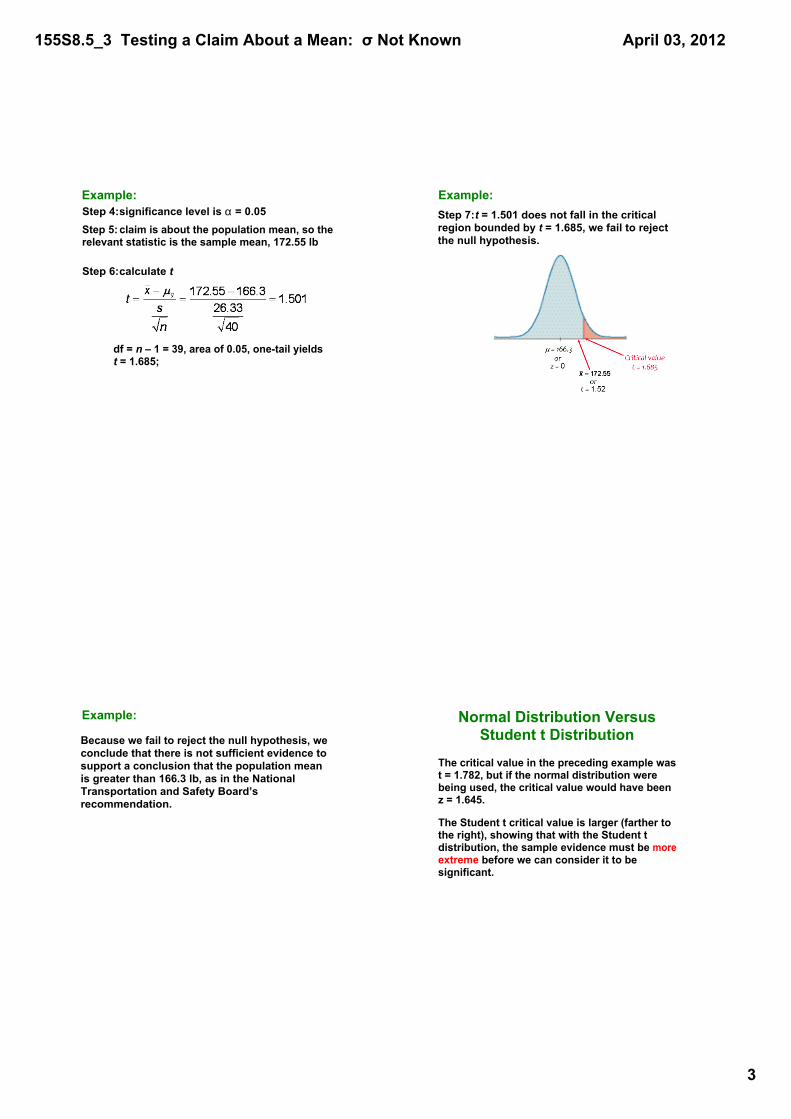
df = n – 1 = 39, area of 0.05, one­tail yields t = 1.685;

Example:Step 7:t = 1.501 does not fall in the critical region bounded by t = 1.685, we fail to reject the null hypothesis.

Example:

Because we fail to reject the null hypothesis, we conclude that there is not sufficient evidence to support a conclusion that the population mean is greater than 166.3 lb, as in the National Transportation and Safety Board’s recommendation.

The critical value in the preceding example was t = 1.782, but if the normal distribution were being used, the critical value would have been z = 1.645.

The Student t critical value is larger (farther to the right), showing that with the Student t distribution, the sample evidence must be more extreme before we can consider it to be significant.

Normal Distribution Versus Student t Distribution

155S8.5_3 Testing a Claim About a Mean: σ Not Known

4

April 03, 2012

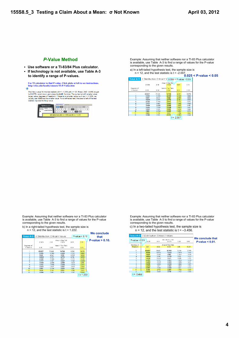
P­Value Method• Use software or a TI­83/84 Plus calculator.• If technology is not available, use Table A­3 to identify a range of P­values.

Use TI calculator to find P­value. Click globe at left to see instructions. http://cfcc.edu/faculty/cmoore/TI­P­Value.htm

Example: Assuming that neither software nor a TI­83 Plus calculator is available, use Table A­3 to find a range of values for the P­value corresponding to the given results.a) In a left­tailed hypothesis test, the sample size is n = 12, and the test statistic is t = ­2.007.

0.025 < P­value < 0.05

Example: Assuming that neither software nor a TI­83 Plus calculator is available, use Table A­3 to find a range of values for the P­value corresponding to the given results.b) In a right­tailed hypothesis test, the sample size is n = 12, and the test statistic is t = 1.222.

We conclude that

P­value > 0.10.

Example: Assuming that neither software nor a TI­83 Plus calculator is available, use Table A­3 to find a range of values for the P­value corresponding to the given results.c) In a two­tailed hypothesis test, the sample size is n = 12, and the test statistic is t = –3.456.

We conclude that P­value < 0.01.

155S8.5_3 Testing a Claim About a Mean: σ Not Known

5

April 03, 2012

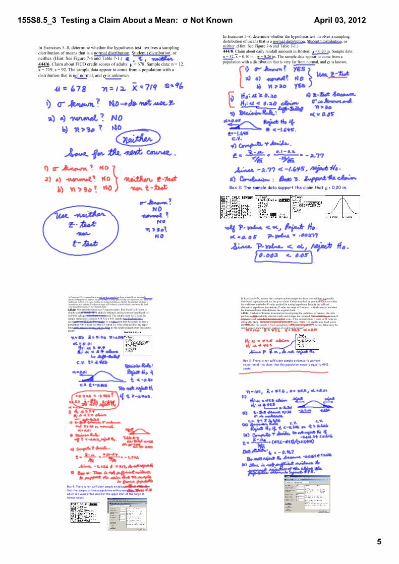
In Exercises 5–8, determine whether the hypothesis test involves a sampling distribution of means that is a normal distribution, Student t distribution, or neither. (Hint: See Figure 7­6 and Table 7­1.)444/6. Claim about FICO credit scores of adults: μ = 678. Sample data: n = 12. x = 719, s = 92. The sample data appear to come from a population with a distribution that is not normal, and σ is unknown.

In Exercises 5–8, determine whether the hypothesis test involves a sampling distribution of means that is a normal distribution, Student t distribution, or neither. (Hint: See Figure 7­6 and Table 7­1.)444/8. Claim about daily rainfall amounts in Boston: μ < 0.20 in. Sample data: n = 52, x = 0.10 in., σ = 0.26 in. The sample data appear to come from a population with a distribution that is very far from normal, and σ is known.

Box 3: The sample data support the claim that μ < 0.20 in.

445/10. Normal distribution; use 5­step procedure. Red Blood Cell Count. A simple random sample of 50 adults is obtained, and each person's red blood cell count (in cells per microliter) is measured. The sample mean is 5.23 and the sample standard deviation is 0.54. Use a 0.01 significance level and the accompanying TI­83/84 Plus display to test the claim that the sample is from a population with a mean less than 5.4 which is a value often used for the upper limit of the range of normal values. What do the results suggest about the sample group?

In Exercises 9­24, assume that a simple random sample has been selected from a normally distributed population and test the given claim. Unless specified by your instructor, use either the traditional method or P­value method for testing hypotheses. Identify the null and alternative hypotheses, test statistic, P­value (or range of P­values), critical value(s), and state the final conclusion that addresses the original claim.

Box 4: There is not sufficient sample evidence to support the claim that the sample is from a population with a mean less than 5.4 which is a value often used for the upper limit of the range of normal values.

In Exercises 9–24, assume that a simple random sample has been selected from a normally distributed population and test the given claim. Unless specified by your instructor, use either the traditional method or P­value method for testing hypotheses. Identify the null and alternative hypotheses, test statistic, P­value (or range of P­values), critical value(s), and state the final conclusion that addresses the original claim.445/14. Analysis of Pennies In an analysis investigating the usefulness of pennies, the cents portions of 100 randomly selected credit card charges are recorded. The sample has a mean of 47.6 cents and a standard deviation of 33.5 cents. If the amounts from 0 cents to 99 cents are all equally likely, the mean is expected to be 49.5 cents. Use a 0.01 significance level to test the claim that the sample is from a population with a mean equal to 49.5 cents. What does the result suggest about the cents portions of credit card charges?

Box 2: There is not sufficient sample evidence to warrant rejection of the claim that the population mean is equal to 49.5 cents.

155S8.5_3 Testing a Claim About a Mean: σ Not Known

6

April 03, 2012

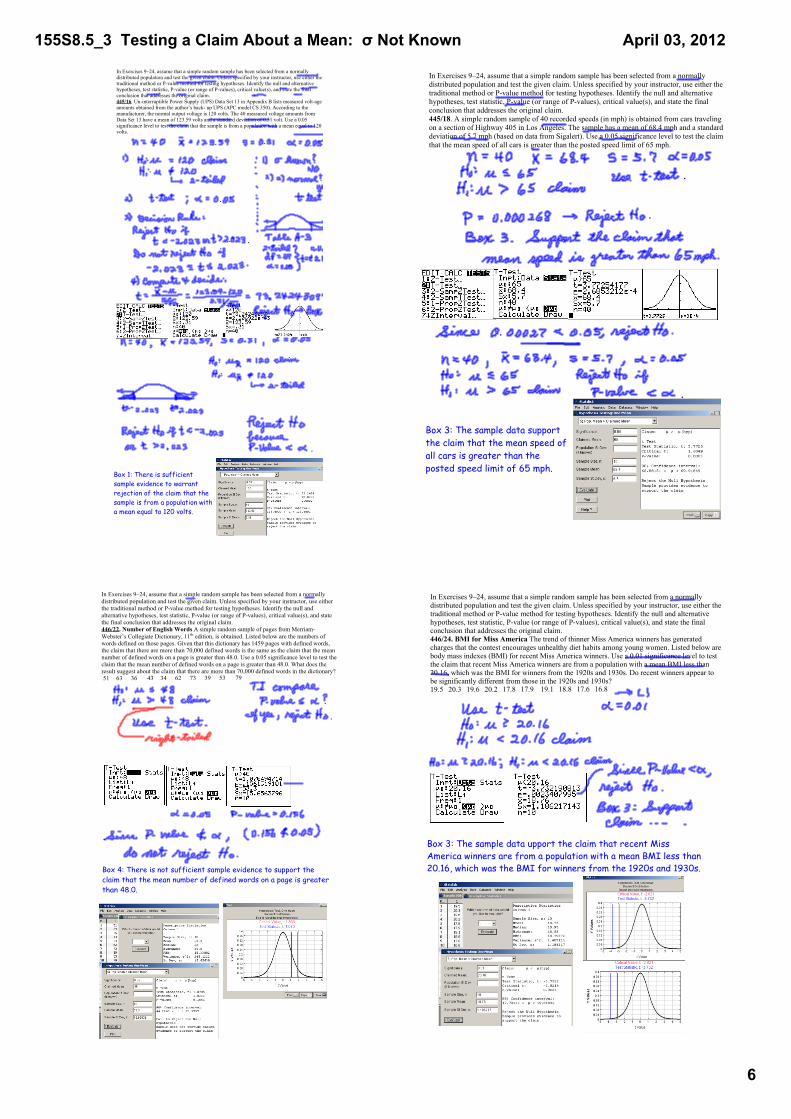
In Exercises 9–24, assume that a simple random sample has been selected from a normally distributed population and test the given claim. Unless specified by your instructor, use either the traditional method or P­value method for testing hypotheses. Identify the null and alternative hypotheses, test statistic, P­value (or range of P­values), critical value(s), and state the final conclusion that addresses the original claim.445/16. Un­interruptible Power Supply (UPS) Data Set 13 in Appendix B lists measured volt­age amounts obtained from the author’s back­ up UPS (APC model CS 350). According to the manufacturer, the normal output voltage is 120 volts. The 40 measured voltage amounts from Data Set 13 have a mean of 123.59 volts and a standard deviation of 0.31 volt. Use a 0.05 significance level to test the claim that the sample is from a population with a mean equal to 120 volts.

Box 1: There is sufficient sample evidence to warrant rejection of the claim that the sample is from a population with a mean equal to 120 volts.

In Exercises 9–24, assume that a simple random sample has been selected from a normally distributed population and test the given claim. Unless specified by your instructor, use either the traditional method or P­value method for testing hypotheses. Identify the null and alternative hypotheses, test statistic, P­value (or range of P­values), critical value(s), and state the final conclusion that addresses the original claim.445/18. A simple random sample of 40 recorded speeds (in mph) is obtained from cars traveling on a section of Highway 405 in Los Angeles. The sample has a mean of 68.4 mph and a standard deviation of 5.7 mph (based on data from Sigalert). Use a 0.05 significance level to test the claim that the mean speed of all cars is greater than the posted speed limit of 65 mph.

Box 3: The sample data support the claim that the mean speed of all cars is greater than the posted speed limit of 65 mph.

In Exercises 9–24, assume that a simple random sample has been selected from a normally distributed population and test the given claim. Unless specified by your instructor, use either the traditional method or P­value method for testing hypotheses. Identify the null and alternative hypotheses, test statistic, P­value (or range of P­values), critical value(s), and state the final conclusion that addresses the original claim.446/22. Number of English Words A simple random sample of pages from Merriam­ Webster’s Collegiate Dictionary, 11th edition, is obtained. Listed below are the numbers of words defined on those pages. Given that this dictionary has 1459 pages with defined words, the claim that there are more than 70,000 defined words is the same as the claim that the mean number of defined words on a page is greater than 48.0. Use a 0.05 significance level to test the claim that the mean number of defined words on a page is greater than 48.0. What does the result suggest about the claim that there are more than 70,000 defined words in the dictionary? 51 63 36 43 34 62 73 39 53 79

Box 4: There is not sufficient sample evidence to support the claim that the mean number of defined words on a page is greater than 48.0.

In Exercises 9–24, assume that a simple random sample has been selected from a normally distributed population and test the given claim. Unless specified by your instructor, use either the traditional method or P­value method for testing hypotheses. Identify the null and alternative hypotheses, test statistic, P­value (or range of P­values), critical value(s), and state the final conclusion that addresses the original claim.446/24. BMI for Miss America The trend of thinner Miss America winners has generated charges that the contest encourages unhealthy diet habits among young women. Listed below are body mass indexes (BMI) for recent Miss America winners. Use a 0.01 significance level to test the claim that recent Miss America winners are from a population with a mean BMI less than 20.16, which was the BMI for winners from the 1920s and 1930s. Do recent winners appear to be significantly different from those in the 1920s and 1930s? 19.5 20.3 19.6 20.2 17.8 17.9 19.1 18.8 17.6 16.8

Box 3: The sample data upport the claim that recent Miss America winners are from a population with a mean BMI less than 20.16, which was the BMI for winners from the 1920s and 1930s.