Revisiting Stock-Recruitment Relationships

Rainer Froese24.02.09

Mini-workshop on Fisheries: Ecology, Economics and Policy

CAU, Kiel, Germany

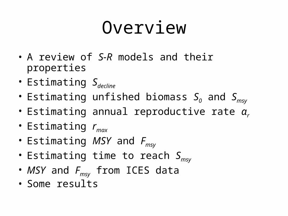
Overview

• A review of S-R models and their properties• Estimating Sdecline

• Estimating unfished biomass S0 and Smsy

• Estimating annual reproductive rate αr

• Estimating rmax • Estimating MSY and Fmsy

• Estimating time to reach Smsy

• MSY and Fmsy from ICES data• Some results

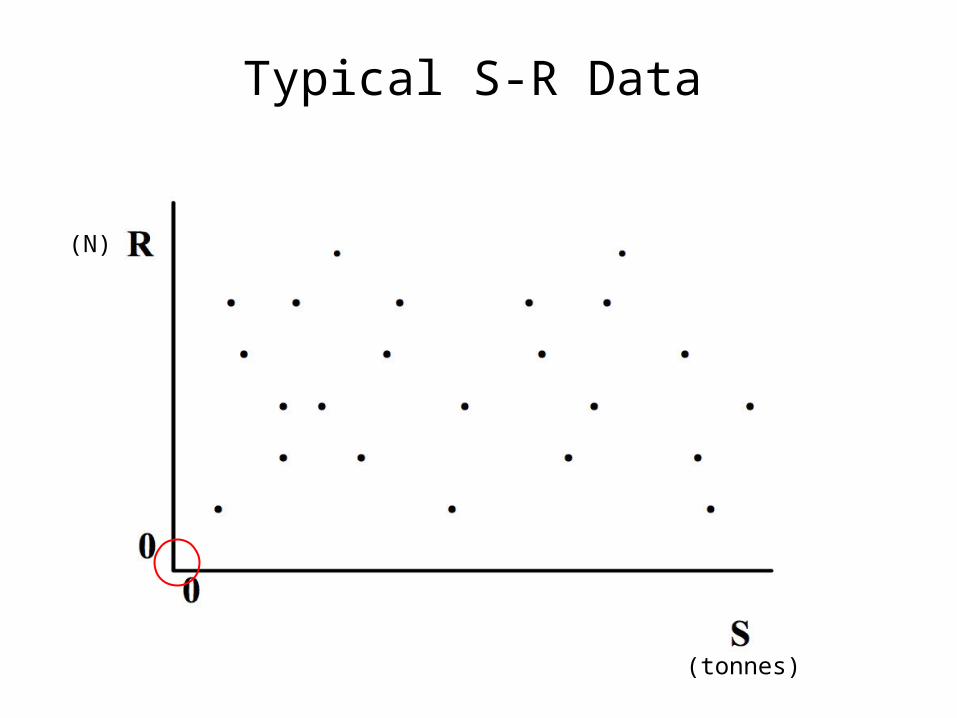
Typical S-R Data

(N)

(tonnes)

0

500

1000

1500

0 1 2 3 4 5

Rnorm

Fre

quency

(n)

0

500

1000

1500

2000

2500

-5 -3 0 3 5

Rnorm

Fre

quency

(n)

0

500

1000

1500

2000

2500

-5.00 -2.50 0.00 2.50 5.00

LNSnorm

Fre

quency

(n)

Skewed roughly log-normal

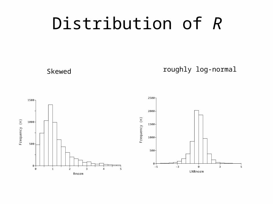
Distribution of R

0

500

1000

1500

2000

2500

-5.00 -2.50 0.00 2.50 5.00

LNSnorm

Fre

quency

(n)

0

500

1000

1500

2000

2500

0 1 3 4 5

Snorm

Fre

quency

(n)

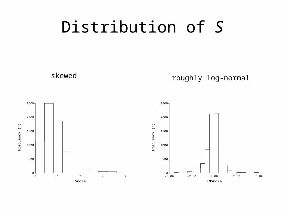
Distribution of S

skewed roughly log-normal

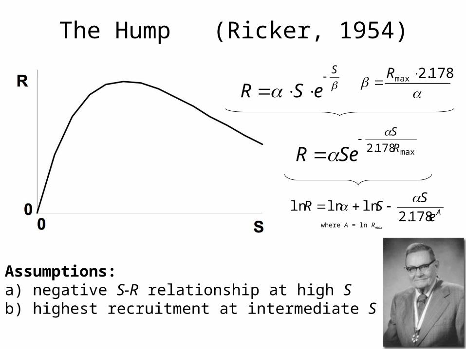
The Hump (Ricker, 1954)

S

eSR

max178.2 R

S

SeR

Ae

SSR

178.2lnlnln

178.2max

R

Assumptions: a) negative S-R relationship at high Sb) highest recruitment at intermediate S

where A = ln Rmax

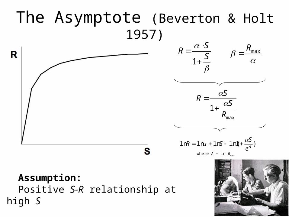
Assumption:Positive S-R relationship at

high S

SS

R

1

maxR

max

1R

SS

R

)1ln(lnlnlnAe

SSR

The Asymptote (Beverton & Holt 1957)

where A = ln Rmax

Spawners (N)

Re

cru

its

(N

)

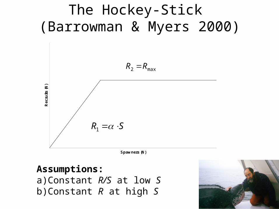
The Hockey-Stick (Barrowman & Myers 2000)

SR 1

max2 RR

Assumptions:a) Constant R/S at low Sb) Constant R at high S

The Smooth Hockey-Stick (Froese 2008)

)1ln(lnS

e AeAR

)1( maxmax

SReRR

Assumptions:a) Practically constant R at high Sb) Gradually increasing R/S at lower S

where A = ln Rmax

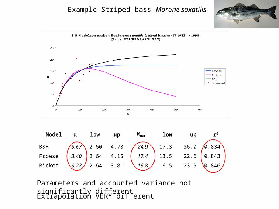
S-R Model comparison for Morone saxatilis (striped bass) n=17 1982 --> 1998[Stock: STRIPEDBASSUSA2]

0

5

10

15

20

25

0 10 20 30 40 50 60

S

R

Froese

Ricker

B&H

observed

Parameters and accounted variance not significantly different

Model α low up Rmax low up r2

B&H 3.67 2.60 4.73 24.9 17.3 36.0 0.834

Froese 3.40 2.64 4.15 17.4 13.5 22.6 0.843

Ricker 3.22 2.64 3.81 19.8 16.5 23.9 0.846

Example Striped bass Morone saxatilis

Extrapolation VERY different

0.01

0.1

1

10

0.01 0.1 1 10

Spawner abundance

Rec

ruit

ab

un

dan

ce

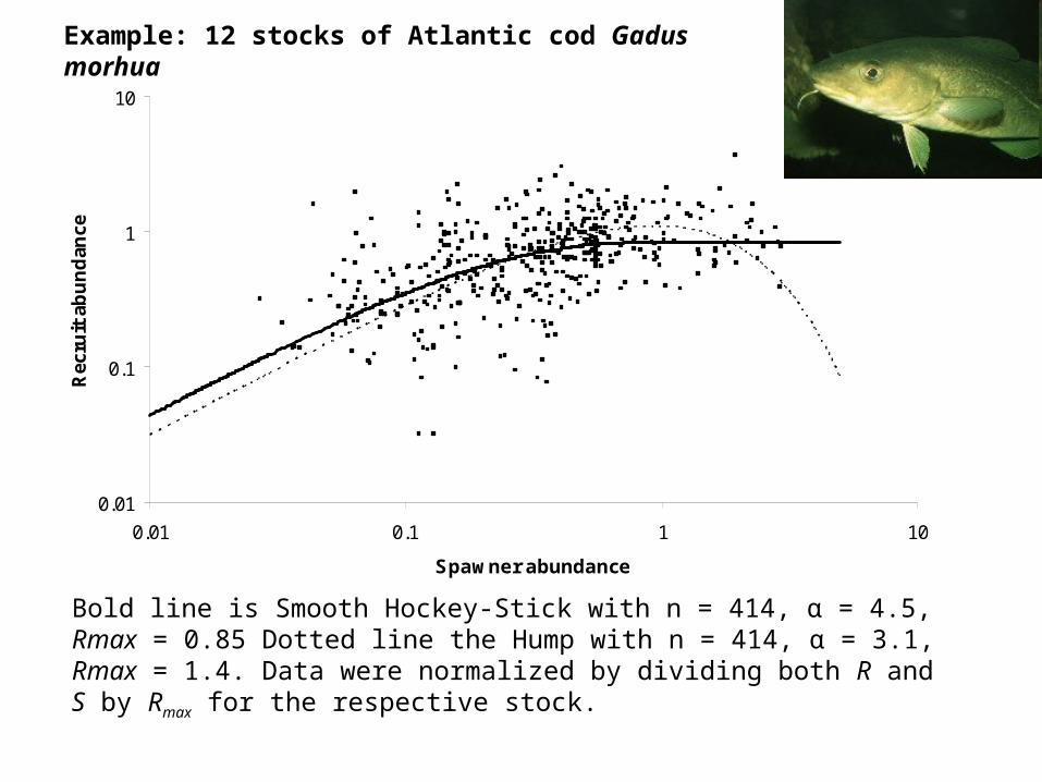
Bold line is Smooth Hockey-Stick with n = 414, α = 4.5, Rmax = 0.85 Dotted line the Hump with n = 414, α = 3.1, Rmax = 1.4. Data were normalized by dividing both R and S by Rmax for the respective stock.

Example: 12 stocks of Atlantic cod Gadus morhua

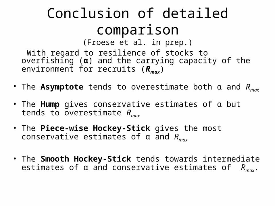
Conclusion of detailed comparison(Froese et al. in prep.)

With regard to resilience of stocks to overfishing (α) and the carrying capacity of the environment for recruits (Rmax)

• The Asymptote tends to overestimate both α and Rmax

• The Hump gives conservative estimates of α but tends to overestimate Rmax

• The Piece-wise Hockey-Stick gives the most conservative estimates of α and Rmax

• The Smooth Hockey-Stick tends towards intermediate estimates of α and conservative estimates of Rmax.

When does R decline?

maxR

Sdecline For the hockey-sticks:

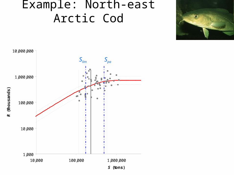
Example: North-east Arctic Cod

1,000

10,000

100,000

1,000,000

10,000,000

10,000 100,000 1,000,000 10,000,000 100,000,000

S (tons)

R (

tho

us

an

ds

)

S decline S msy Slim Spa Smax

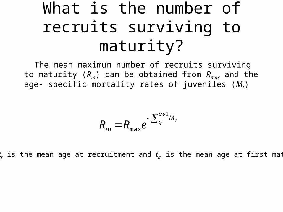
What is the number of recruits surviving to maturity?

The mean maximum number of recruits surviving to maturity (Rm) can be obtained from Rmax and the age- specific mortality rates of juveniles (Mt)

1

max

tm

rttM

m eRR

where tr is the mean age at recruitment and tm is the mean age at first maturity

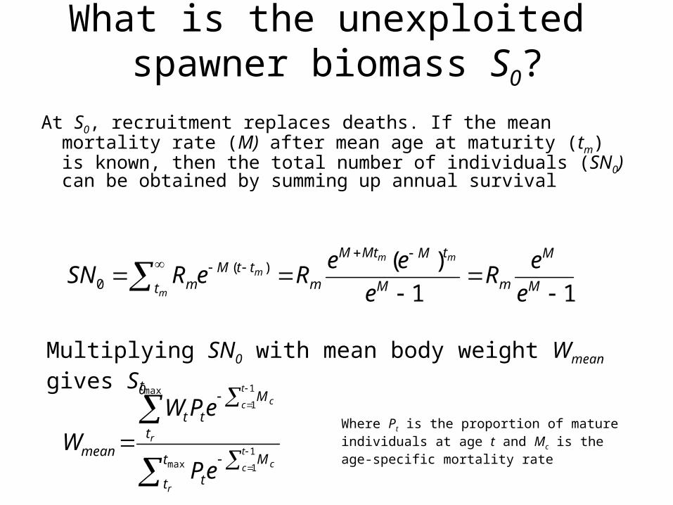
What is the unexploited spawner biomass S0?

At S0, recruitment replaces deaths. If the mean mortality rate (M) after mean age at maturity (tm) is known, then the total number of individuals (SN0) can be obtained by summing up annual survival

Multiplying SN0 with mean body weight Wmean gives S0

11

)()(0

M

M

mM

tMMtM

mt

ttMm e

eR

e

eeReRSN

mm

m

m

max1

1

max 1

1

t

t

M

t

t

t

M

tt

mean

r

t

c c

r

t

c c

eP

ePW

WWhere Pt is the proportion of matureindividuals at age t and Mc is the age-specific mortality rate

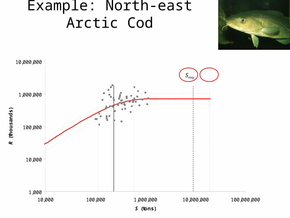
Example: North-east Arctic Cod

1,000

10,000

100,000

1,000,000

10,000,000

10,000 100,000 1,000,000 10,000,000 100,000,000

S (tons)

R (

tho

us

an

ds

)

S decline S 0Smsy

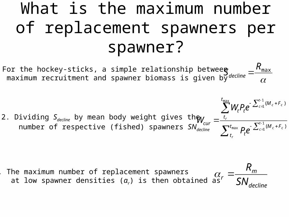
What is the maximum number of replacement spawners per spawner?

maxR

Sdecline 1. For the hockey-sticks, a simple relationship between maximum recruitment and spawner biomass is given by

2. Dividing Sdecline by mean body weight gives the number of respective (fished) spawners SNdecline

max1

1

max 1

1

)(

)(

t

t

FM

t

t

t

FM

tt

cur

r

t

c cc

r

t

c cc

eP

ePW

W

3. The maximum number of replacement spawners at low spawner densities (αr) is then obtained as

decline

mr SN

R

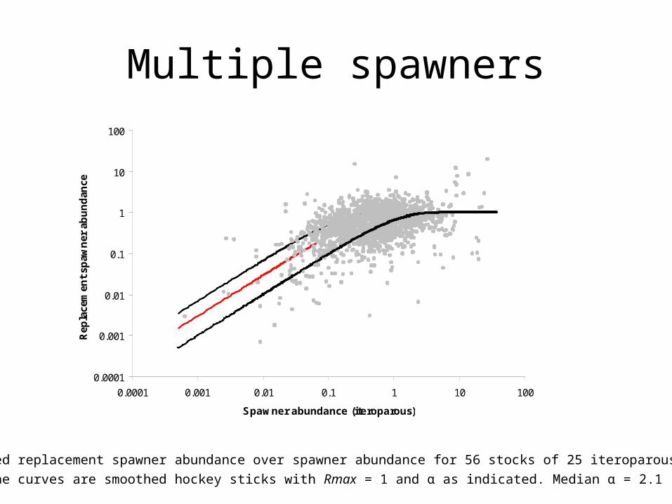
Multiple spawners

0.0001

0.001

0.01

0.1

1

10

100

0.0001 0.001 0.01 0.1 1 10 100

Spawner abundance (iteroparous)

Rep

lace

men

t sp

awn

er a

bu

nd

ance

α=7α=3

α=1

Standardized replacement spawner abundance over spawner abundance for 56 stocks of 25 iteroparous

species. The curves are smoothed hockey sticks with Rmax = 1 and α as indicated. Median α = 2.1 (1.7 – 2.8).

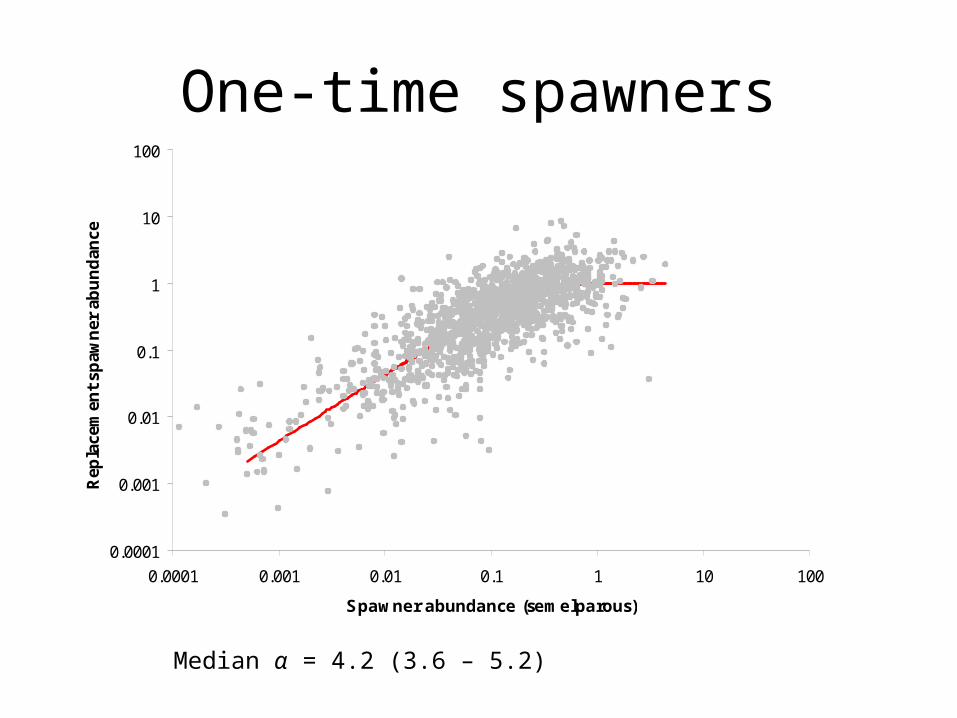
One-time spawners

Median α = 4.2 (3.6 – 5.2)

0.0001

0.001

0.01

0.1

1

10

100

0.0001 0.001 0.01 0.1 1 10 100

Spawner abundance (semelparous)

Rep

lace

men

t sp

awn

er a

bu

nd

ance

α=4.2

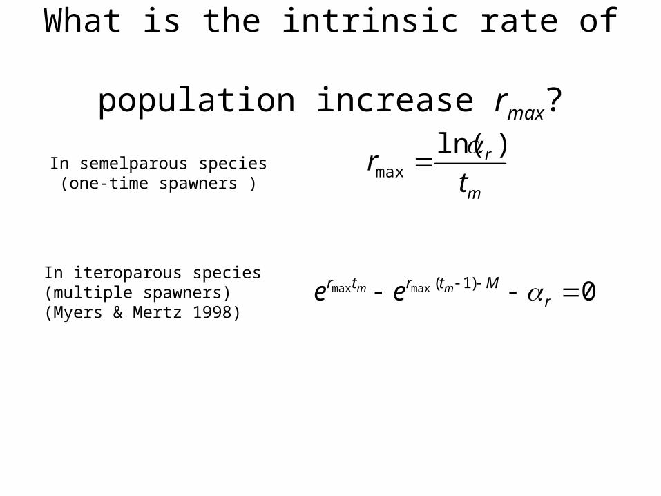
What is the intrinsic rate of population increase rmax?

In semelparous species (one-time spawners )

In iteroparous species(multiple spawners)(Myers & Mertz 1998)

m

r

tr

)ln(max

0)1(maxmax r

Mtrtr mm ee

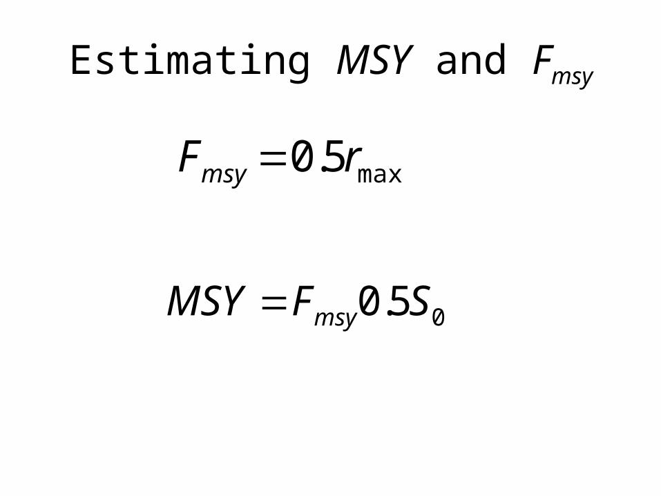
Estimating MSY and Fmsy

max5.0 rFmsy

05.0 SFMSY msy

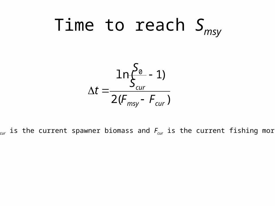
Time to reach Smsy

)(2

)1ln( 0

curmsy

cur

FF

SS

t

where Scur is the current spawner biomass and Fcur is the current fishing mortality

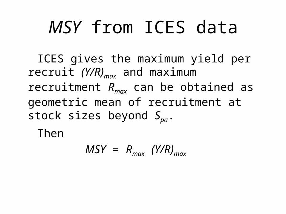
MSY from ICES data

ICES gives the maximum yield per recruit (Y/R)max and maximum recruitment Rmax can be obtained as geometric mean of recruitment at stock sizes beyond Spa.

Then

MSY = Rmax (Y/R)max

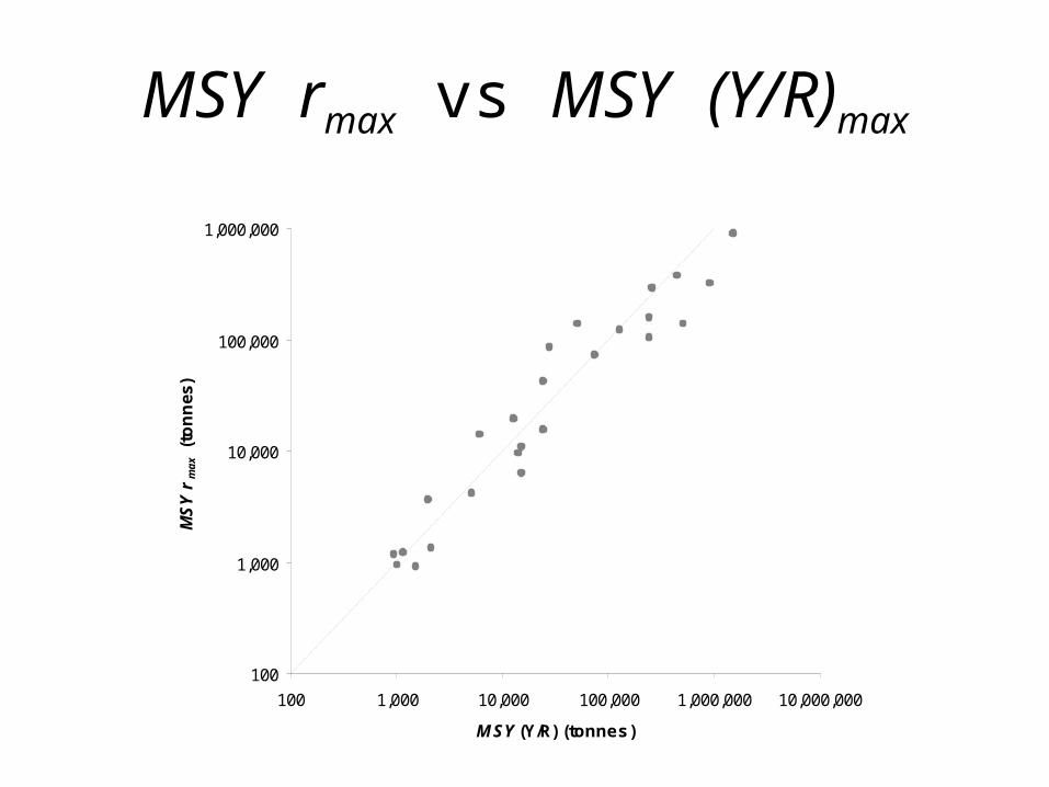
MSY rmax vs MSY (Y/R)max

100

1,000

10,000

100,000

1,000,000

100 1,000 10,000 100,000 1,000,000 10,000,000

M SY (Y/R) (tonnes)

MS

Y r

ma

x (

ton

nes

)

1:1

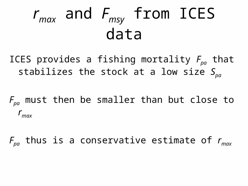
rmax and Fmsy from ICES data

ICES provides a fishing mortality Fpa that stabilizes the stock at a low size Spa

Fpa must then be smaller than but close to rmax

Fpa thus is a conservative estimate of rmax

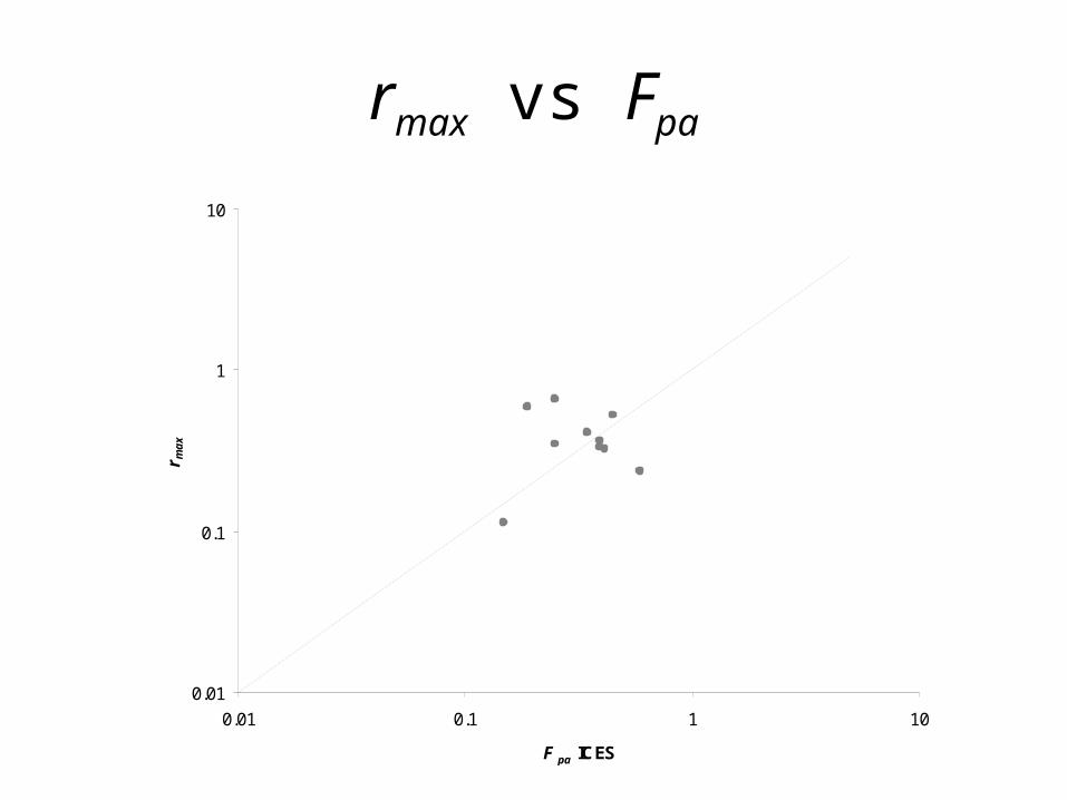
rmax vs Fpa

0.01

0.1

1

10

0.01 0.1 1 10

F pa ICES

r ma

x

1 : 1

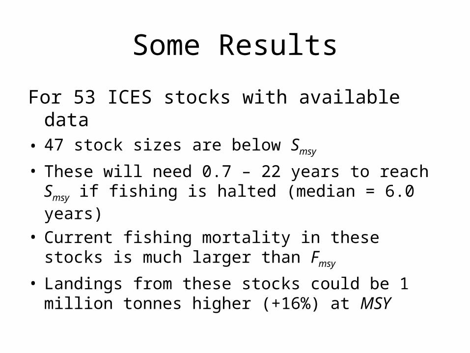
Some Results

For 53 ICES stocks with available data• 47 stock sizes are below Smsy

• These will need 0.7 – 22 years to reach Smsy if fishing is halted (median = 6.0 years)

• Current fishing mortality in these stocks is much larger than Fmsy

• Landings from these stocks could be 1 million tonnes higher (+16%) at MSY

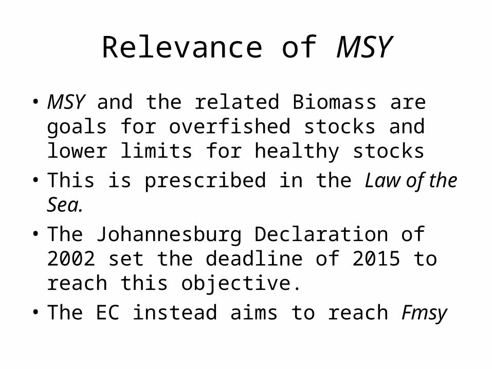
Relevance of MSY

• MSY and the related Biomass are goals for overfished stocks and lower limits for healthy stocks

• This is prescribed in the Law of the Sea.

• The Johannesburg Declaration of 2002 set the deadline of 2015 to reach this objective.

• The EC instead aims to reach Fmsy

Thank You