Recent advances in computing correlationfunctions of the XXZ spin chain

Jean Michel Maillet

CNRS & ENS Lyon

Collaborators : J. S. Caux, N. Kitanine, N. A. Slavnov, V. Terras

– Typeset by FoilTEX – Annecy, September 2005

J. M. Maillet Correlation functions

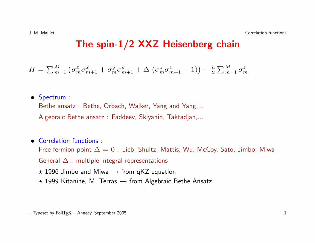
The spin-1/2 XXZ Heisenberg chain

H =∑M

m=1

(σxmσ

xm+1 + σymσ

ym+1 + ∆ (σzmσ

zm+1 − 1)

)− h

2

∑Mm=1 σ

zm

• Spectrum :

Bethe ansatz : Bethe, Orbach, Walker, Yang and Yang,...

Algebraic Bethe ansatz : Faddeev, Sklyanin, Taktadjan,...

• Correlation functions :

Free fermion point ∆ = 0 : Lieb, Shultz, Mattis, Wu, McCoy, Sato, Jimbo, Miwa

General ∆ : multiple integral representations

? 1996 Jimbo and Miwa→ from qKZ equation

? 1999 Kitanine, M, Terras→ from Algebraic Bethe Ansatz

– Typeset by FoilTEX – Annecy, September 2005 1

J. M. Maillet Correlation functions

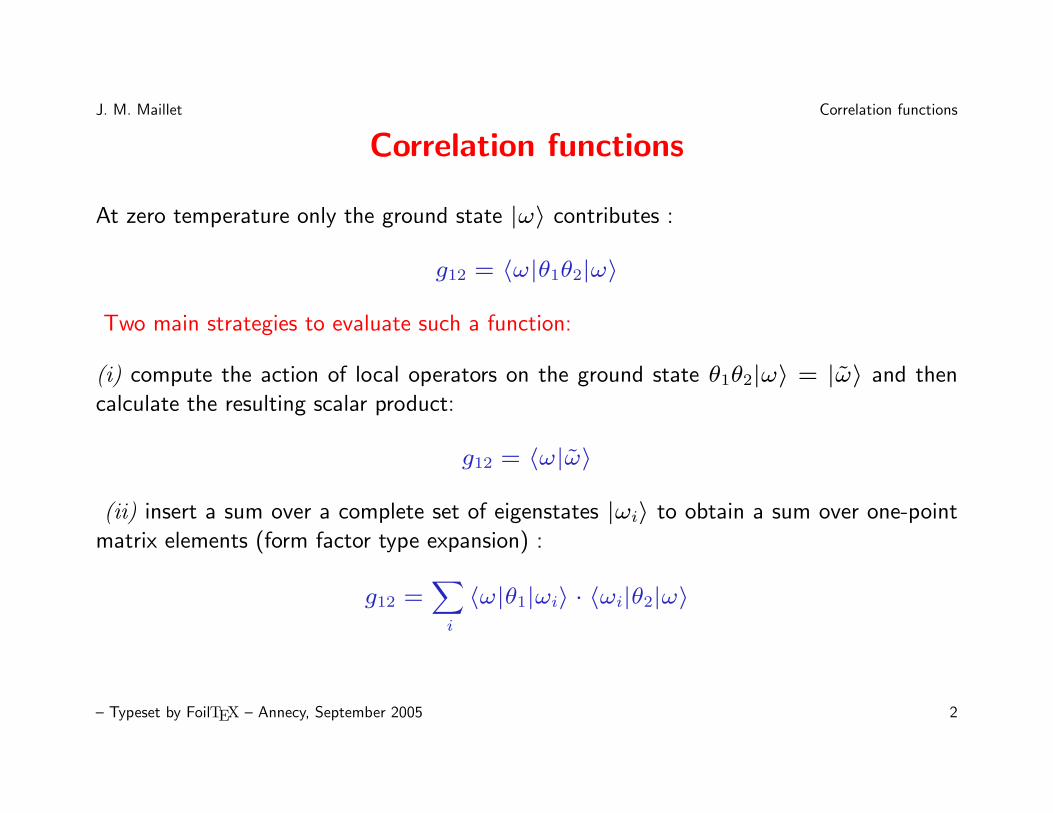
Correlation functions

At zero temperature only the ground state |ω〉 contributes :

g12 = 〈ω|θ1θ2|ω〉

Two main strategies to evaluate such a function:

(i) compute the action of local operators on the ground state θ1θ2|ω〉 = |ω〉 and then

calculate the resulting scalar product:

g12 = 〈ω|ω〉

(ii) insert a sum over a complete set of eigenstates |ωi〉 to obtain a sum over one-point

matrix elements (form factor type expansion) :

g12 =∑i

〈ω|θ1|ωi〉 · 〈ωi|θ2|ω〉

– Typeset by FoilTEX – Annecy, September 2005 2

J. M. Maillet Correlation functions

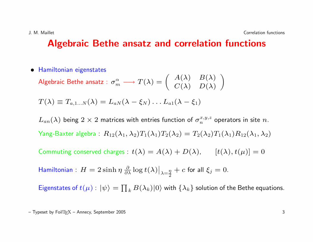
Algebraic Bethe ansatz and correlation functions

• Hamiltonian eigenstates

Algebraic Bethe ansatz : σαm −→ T (λ) =

(A(λ) B(λ)

C(λ) D(λ)

)T (λ) ≡ Ta,1...N(λ) = LaN(λ− ξN) . . . La1(λ− ξ1)

Lan(λ) being 2× 2 matrices with entries function of σx,y,zn operators in site n.

Yang-Baxter algebra : R12(λ1, λ2)T1(λ1)T2(λ2) = T2(λ2)T1(λ1)R12(λ1, λ2)

Commuting conserved charges : t(λ) = A(λ) +D(λ), [t(λ), t(µ)] = 0

Hamiltonian : H = 2 sinh η ∂∂λ log t(λ)

∣∣λ=

η2

+ c for all ξj = 0.

Eigenstates of t(µ) : |ψ〉 =∏

kB(λk)|0〉 with λk solution of the Bethe equations.

– Typeset by FoilTEX – Annecy, September 2005 3

J. M. Maillet Correlation functions

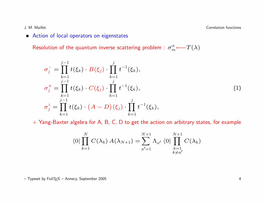
• Action of local operators on eigenstates

Resolution of the quantum inverse scattering problem : σαm←−T (λ)

σ−j =

j−1∏k=1

t(ξk) · B(ξj) ·j∏

k=1

t−1

(ξk),

σ+j =

j−1∏k=1

t(ξk) · C(ξj) ·j∏

k=1

t−1

(ξk),

σzj =

j−1∏k=1

t(ξk) ·(A−D

)(ξj) ·

j∏k=1

t−1

(ξk),

(1)

+ Yang-Baxter algebra for A, B, C, D to get the action on arbitrary states, for example

〈0|N∏k=1

C(λk)A(λN+1) =N+1∑a′=1

Λa′ 〈0|N+1∏k=1k 6=a′

C(λk)

– Typeset by FoilTEX – Annecy, September 2005 4

J. M. Maillet Correlation functions

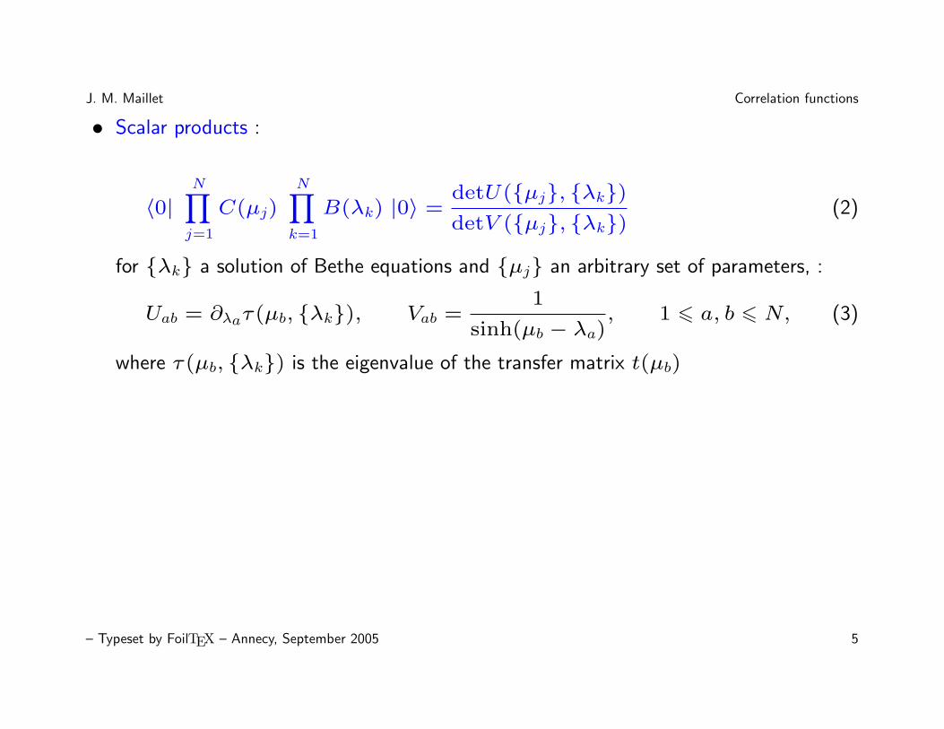
• Scalar products :

〈0|N∏j=1

C(µj)

N∏k=1

B(λk) |0〉 =detU(µj, λk)detV (µj, λk)

(2)

for λk a solution of Bethe equations and µj an arbitrary set of parameters, :

Uab = ∂λaτ(µb, λk), Vab =1

sinh(µb − λa), 1 6 a, b 6 N, (3)

where τ(µb, λk) is the eigenvalue of the transfer matrix t(µb)

– Typeset by FoilTEX – Annecy, September 2005 5

J. M. Maillet Correlation functions

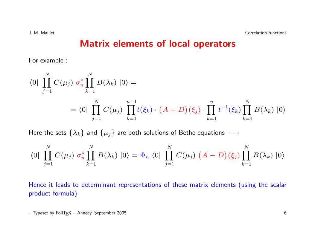
Matrix elements of local operators

For example :

〈0|N∏j=1

C(µj) σzn

N∏k=1

B(λk) |0〉 =

= 〈0|N∏j=1

C(µj)n−1∏k=1

t(ξk) ·(A−D

)(ξj) ·

n∏k=1

t−1

(ξk)

N∏k=1

B(λk) |0〉

Here the sets λk and µj are both solutions of Bethe equations −→

〈0|N∏j=1

C(µj) σzn

N∏k=1

B(λk) |0〉 = Φn 〈0|N∏j=1

C(µj)(A−D

)(ξj)

N∏k=1

B(λk) |0〉

Hence it leads to determinant representations of these matrix elements (using the scalar

product formula)

– Typeset by FoilTEX – Annecy, September 2005 6

J. M. Maillet Correlation functions

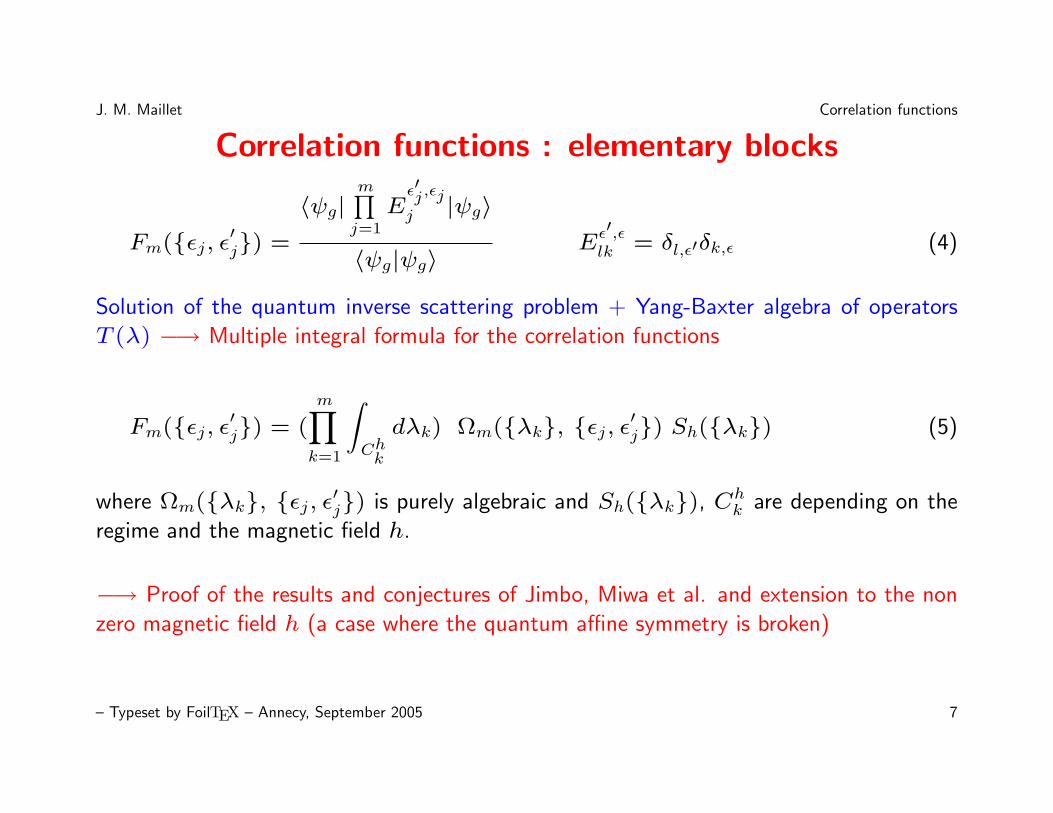
Correlation functions : elementary blocks

Fm(εj, ε′j) =

〈ψg|m∏j=1

Eε′j,εjj |ψg〉

〈ψg|ψg〉Eε′,εlk = δl,ε′δk,ε (4)

Solution of the quantum inverse scattering problem + Yang-Baxter algebra of operators

T (λ) −→ Multiple integral formula for the correlation functions

Fm(εj, ε′j) = (

m∏k=1

∫Chk

dλk) Ωm(λk, εj, ε′j) Sh(λk) (5)

where Ωm(λk, εj, ε′j) is purely algebraic and Sh(λk), Chk are depending on the

regime and the magnetic field h.

−→ Proof of the results and conjectures of Jimbo, Miwa et al. and extension to the non

zero magnetic field h (a case where the quantum affine symmetry is broken)

– Typeset by FoilTEX – Annecy, September 2005 7

J. M. Maillet Correlation functions

What about this result ?

→ A priori, the problem is solved:

• expression of all elementary blocks 〈ψg|Eε′1,ε11 . . . Eε′m,εm

m |ψg〉• any correlation function =

∑(elementary blocks)

→ From a practical point of view, there are two main problems:

(1) physical correlation function = huge sum of elementary blocks at large distances

Example: two-point function

〈ψg|σz1 σzm|ψg〉≡ 〈ψg|(E

111 − E

221 )

m−1∏j=2

(E11j + E

22j )︸ ︷︷ ︸

propagator

(E11m − E

22m )|ψg〉

=∑

2m terms

(elementary blocks) ∼m→∞

?

; re-summation

– Typeset by FoilTEX – Annecy, September 2005 8

J. M. Maillet Correlation functions

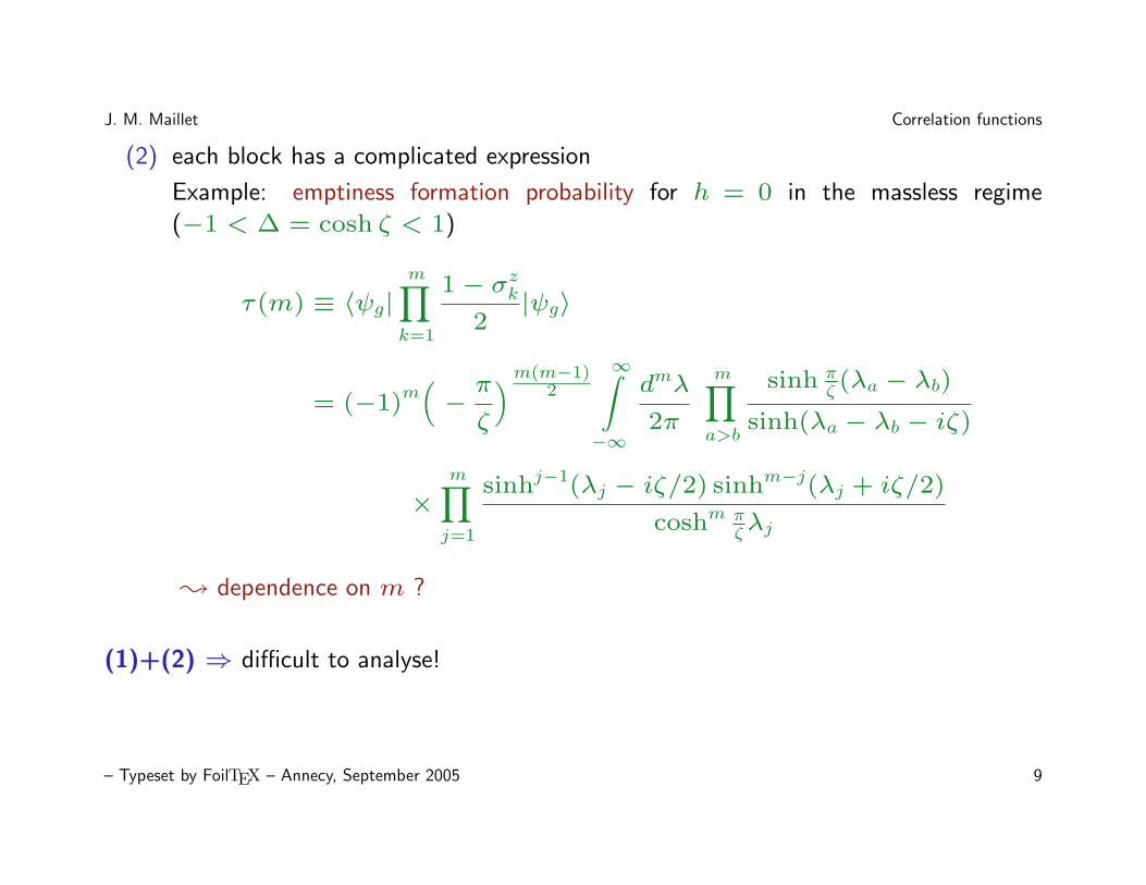
(2) each block has a complicated expression

Example: emptiness formation probability for h = 0 in the massless regime

(−1 < ∆ = cosh ζ < 1)

τ(m) ≡ 〈ψg|m∏k=1

1− σzk2|ψg〉

= (−1)m(−π

ζ

)m(m−1)2

∞∫−∞

dmλ

2π

m∏a>b

sinh πζ (λa − λb)

sinh(λa − λb − iζ)

×m∏j=1

sinhj−1(λj − iζ/2) sinhm−j(λj + iζ/2)

coshm πζλj

; dependence on m ?

(1)+(2) ⇒ difficult to analyse!

– Typeset by FoilTEX – Annecy, September 2005 9

J. M. Maillet Correlation functions

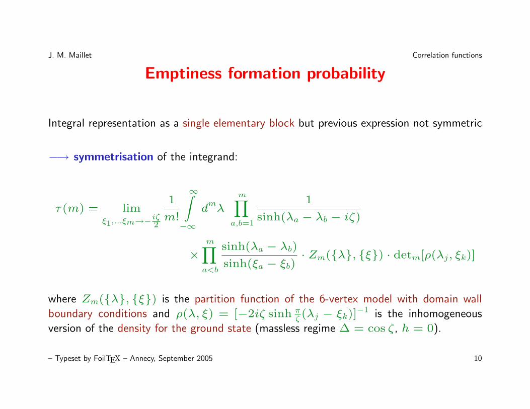
Emptiness formation probability

Integral representation as a single elementary block but previous expression not symmetric

−→ symmetrisation of the integrand:

τ(m) = limξ1,...ξm→−

iζ2

1

m!

∞∫−∞

dmλ

m∏a,b=1

1

sinh(λa − λb − iζ)

×m∏a<b

sinh(λa − λb)sinh(ξa − ξb)

· Zm(λ, ξ) · detm[ρ(λj, ξk)]

where Zm(λ, ξ) is the partition function of the 6-vertex model with domain wall

boundary conditions and ρ(λ, ξ) = [−2iζ sinh πζ (λj − ξk)]

−1 is the inhomogeneous

version of the density for the ground state (massless regime ∆ = cos ζ, h = 0).

– Typeset by FoilTEX – Annecy, September 2005 10

J. M. Maillet Correlation functions

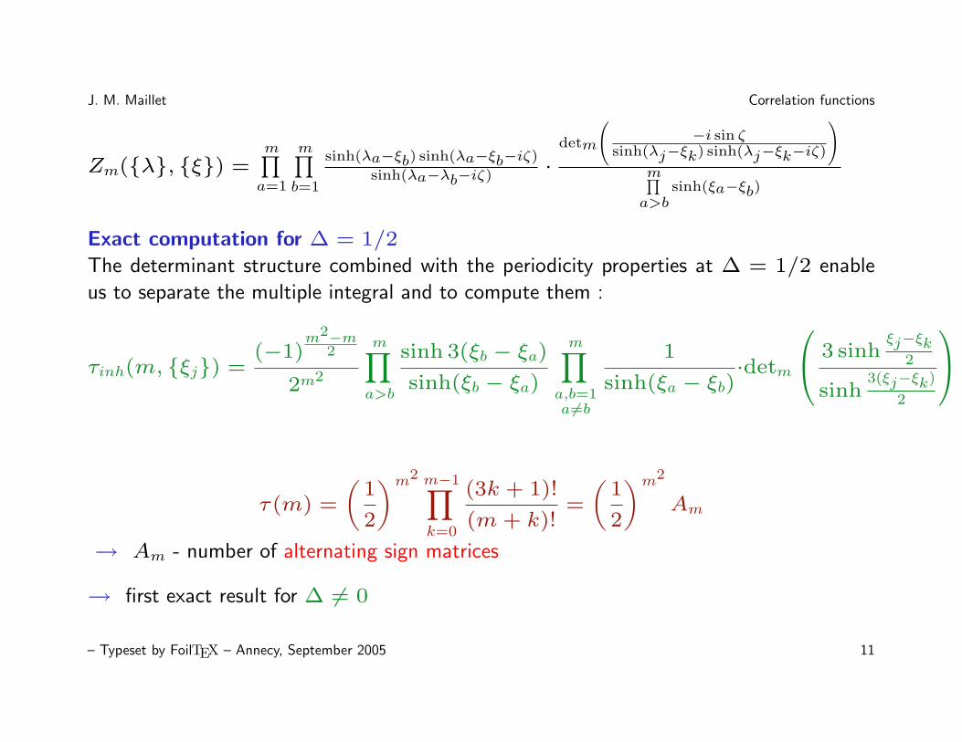
Zm(λ, ξ) =m∏a=1

m∏b=1

sinh(λa−ξb) sinh(λa−ξb−iζ)sinh(λa−λb−iζ)

·detm

(−i sin ζ

sinh(λj−ξk) sinh(λj−ξk−iζ)

)m∏a>b

sinh(ξa−ξb)

Exact computation for ∆ = 1/2

The determinant structure combined with the periodicity properties at ∆ = 1/2 enable

us to separate the multiple integral and to compute them :

τinh(m, ξj) =(−1)

m2−m2

2m2

m∏a>b

sinh 3(ξb − ξa)sinh(ξb − ξa)

m∏a,b=1a6=b

1

sinh(ξa − ξb)·detm

3 sinhξj−ξk

2

sinh3(ξj−ξk)

2

.

τ(m) =

(1

2

)m2 m−1∏k=0

(3k + 1)!

(m+ k)!=

(1

2

)m2

Am

→ Am - number of alternating sign matrices

→ first exact result for ∆ 6= 0

– Typeset by FoilTEX – Annecy, September 2005 11

J. M. Maillet Correlation functions

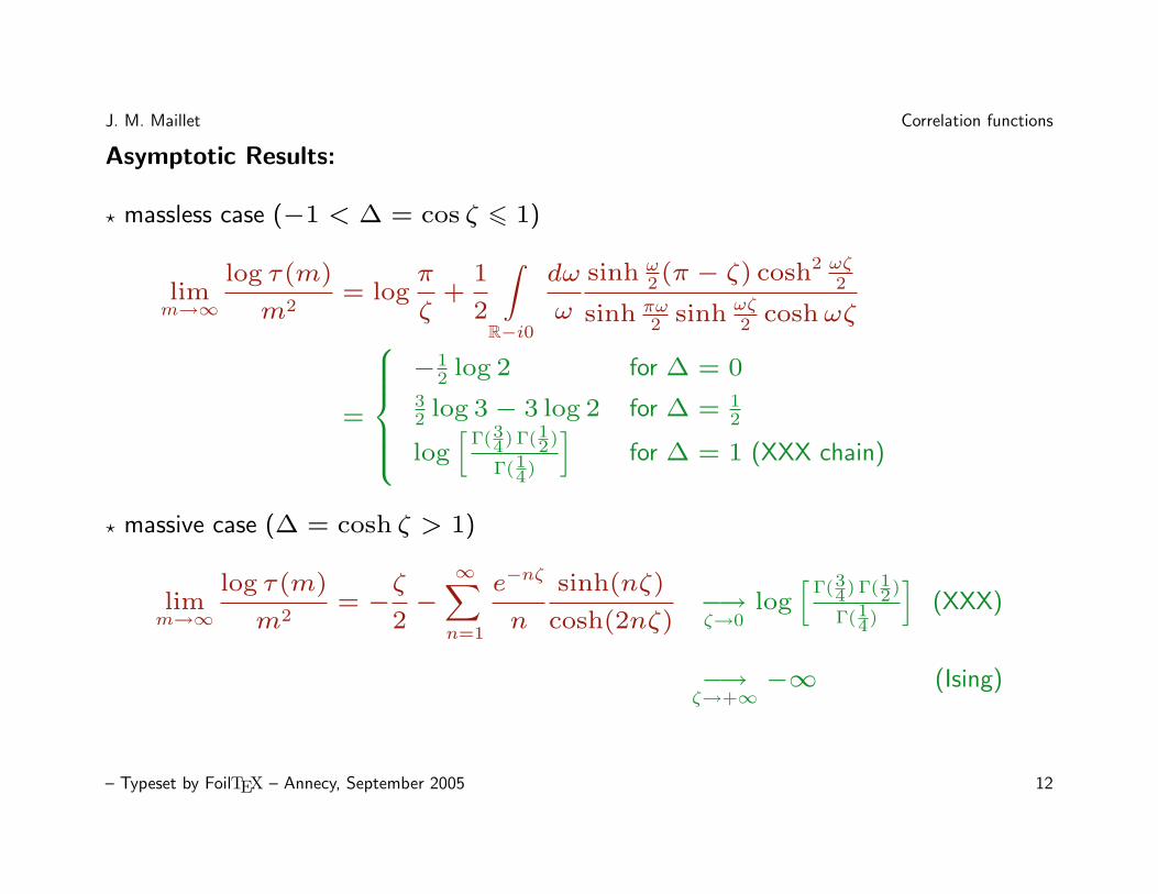
Asymptotic Results:

? massless case (−1 < ∆ = cos ζ 6 1)

limm→∞

log τ(m)

m2= log

π

ζ+

1

2

∫R−i0

dω

ω

sinh ω2 (π − ζ) cosh2 ωζ

2

sinh πω2 sinh ωζ

2 coshωζ

=

−1

2 log 2 for ∆ = 032 log 3− 3 log 2 for ∆ = 1

2

log[

Γ(34) Γ(12)

Γ(14)

]for ∆ = 1 (XXX chain)

? massive case (∆ = cosh ζ > 1)

limm→∞

log τ(m)

m2= −

ζ

2−∞∑n=1

e−nζ

n

sinh(nζ)

cosh(2nζ)−→ζ→0

log[

Γ(34) Γ(12)

Γ(14)

](XXX)

−→ζ→+∞

−∞ (Ising)

– Typeset by FoilTEX – Annecy, September 2005 12

J. M. Maillet Correlation functions

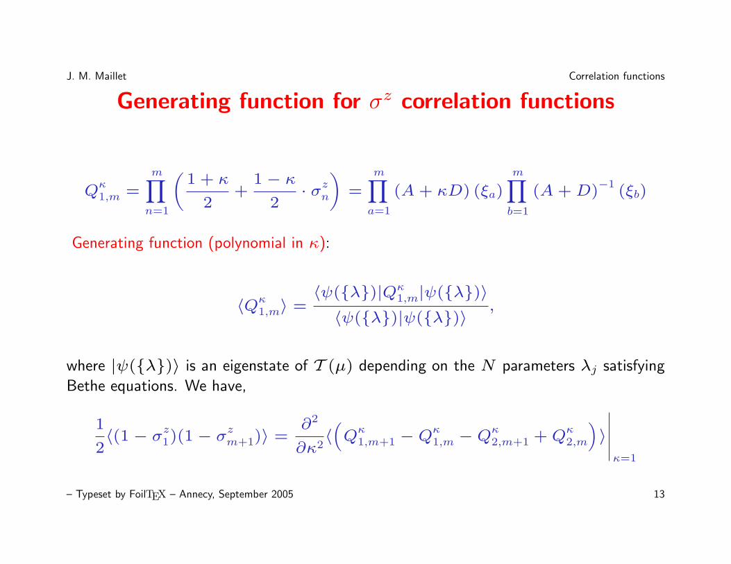
Generating function for σz correlation functions

Qκ1,m =

m∏n=1

(1 + κ

2+

1− κ2· σzn)

=m∏a=1

(A+ κD) (ξa)m∏b=1

(A+D)−1

(ξb)

Generating function (polynomial in κ):

〈Qκ1,m〉 =

〈ψ(λ)|Qκ1,m|ψ(λ)〉

〈ψ(λ)|ψ(λ)〉,

where |ψ(λ)〉 is an eigenstate of T (µ) depending on the N parameters λj satisfying

Bethe equations. We have,

1

2〈(1− σz1)(1− σ

zm+1)〉 =

∂2

∂κ2〈(Qκ1,m+1 −Q

κ1,m −Q

κ2,m+1 +Q

κ2,m

)〉

∣∣∣∣∣κ=1

– Typeset by FoilTEX – Annecy, September 2005 13

J. M. Maillet Correlation functions

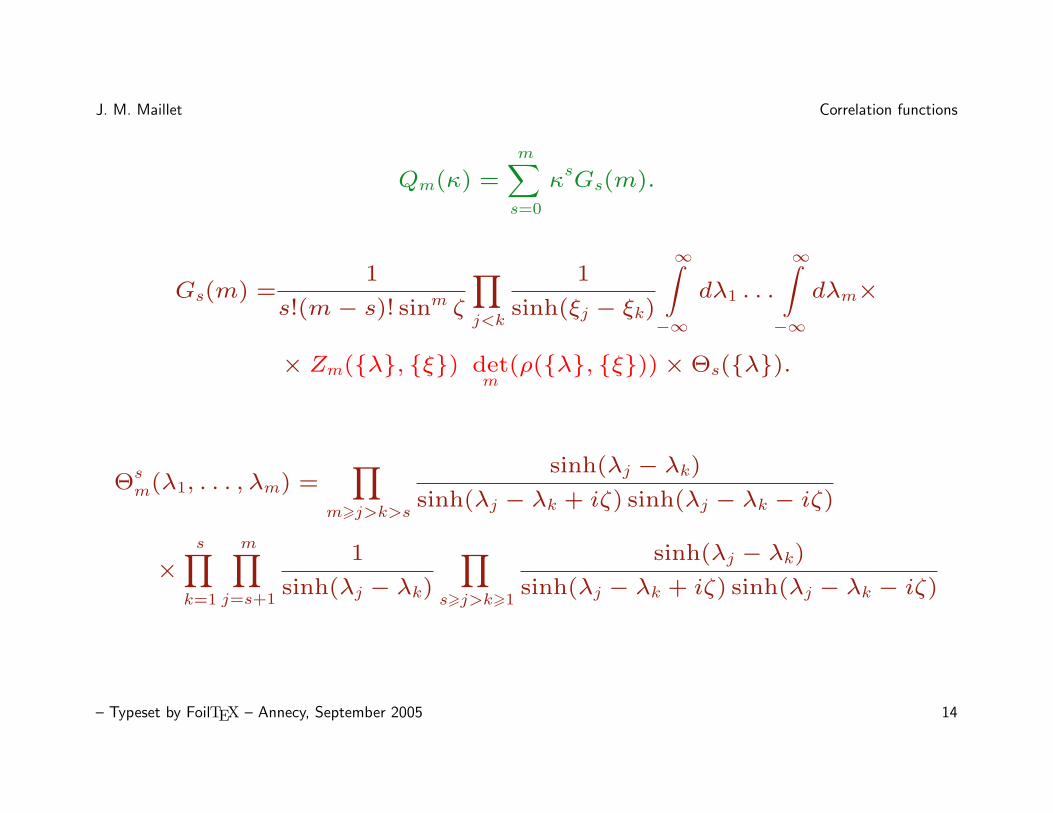
Qm(κ) =

m∑s=0

κsGs(m).

Gs(m) =1

s!(m− s)! sinm ζ∏j<k

1

sinh(ξj − ξk)

∞∫−∞

dλ1 . . .

∞∫−∞

dλm×

× Zm(λ, ξ) detm

(ρ(λ, ξ))×Θs(λ).

Θsm(λ1, . . . , λm) =

∏m>j>k>s

sinh(λj − λk)sinh(λj − λk + iζ) sinh(λj − λk − iζ)

×s∏

k=1

m∏j=s+1

1

sinh(λj − λk)∏

s>j>k>1

sinh(λj − λk)sinh(λj − λk + iζ) sinh(λj − λk − iζ)

– Typeset by FoilTEX – Annecy, September 2005 14

J. M. Maillet Correlation functions

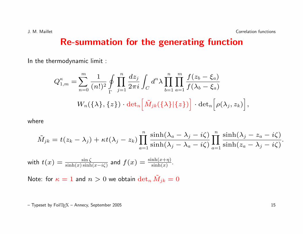
Re-summation for the generating function

In the thermodynamic limit :

Qκ1,m =

m∑n=0

1

(n!)2

∮Γ

n∏j=1

dzj

2πi

∫C

dnλ

n∏b=1

m∏a=1

f(zb − ξa)f(λb − ξa)

Wn(λ, z) · detn[Mjk(λ|z)

]· detn

[ρ(λj, zk)

],

where

Mjk = t(zk − λj) + κt(λj − zk)n∏a=1

sinh(λa − λj − iζ)sinh(λj − λa − iζ)

n∏a=1

sinh(λj − za − iζ)sinh(za − λj − iζ)

.

with t(x) = sin ζsinh(x) sinh(x−iζ) and f(x) = sinh(x+η)

sinh(x) .

Note: for κ = 1 and n > 0 we obtain detn Mjk = 0

– Typeset by FoilTEX – Annecy, September 2005 15

J. M. Maillet Correlation functions

Master equation for σz correlation functions

Let the inhomogeneities ξ be generic and the set λ be an admissible off-diagonal

solution of the Bethe equations (cf.Tarasov - Varchenko). Then there exists κ0 > 0 such,

that for |κ| < κ0 the expectation value of the operator Qκ1,m :

〈Qκ1,m〉 =

1

N !

∮Γξ∪Γλ

N∏j=1

dzj

2πi·

N∏a,b=1

sinh2(λa − zb) ·

m∏a=1

τκ(ξa|z)τ(ξa|λ)

×detN

(∂τκ(λj|z)

∂zk

)· detN

(∂τ(zk|λ)

∂λj

)N∏a=1Yκ(za|z) · detN

(∂Y(λk|λ)

∂λj

) .

The integration contour is such that the only singularities of the integrand within the

contour Γξ ∪ Γλ which contribute to the integral are the points ξ and λ(hep-th/0406190).

– Typeset by FoilTEX – Annecy, September 2005 16

J. M. Maillet Correlation functions

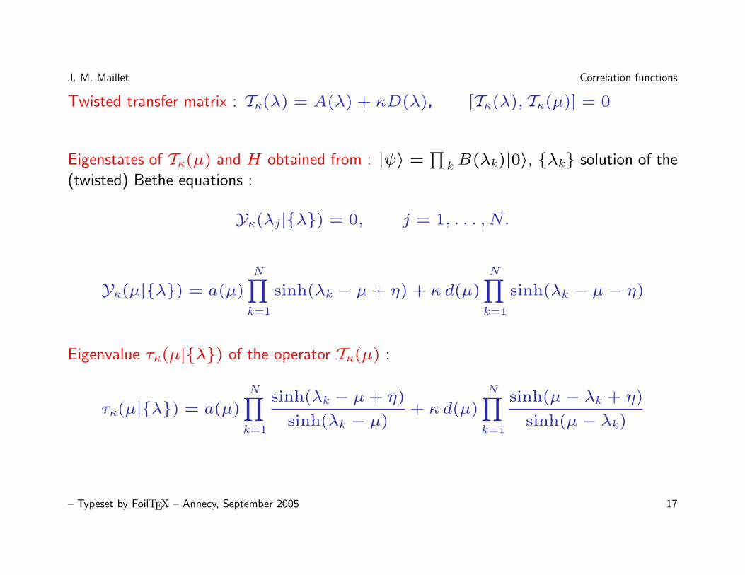
Twisted transfer matrix : Tκ(λ) = A(λ) + κD(λ), [Tκ(λ), Tκ(µ)] = 0

Eigenstates of Tκ(µ) and H obtained from : |ψ〉 =∏

kB(λk)|0〉, λk solution of the

(twisted) Bethe equations :

Yκ(λj|λ) = 0, j = 1, . . . , N.

Yκ(µ|λ) = a(µ)

N∏k=1

sinh(λk − µ+ η) + κ d(µ)

N∏k=1

sinh(λk − µ− η)

Eigenvalue τκ(µ|λ) of the operator Tκ(µ) :

τκ(µ|λ) = a(µ)N∏k=1

sinh(λk − µ+ η)

sinh(λk − µ)+ κ d(µ)

N∏k=1

sinh(µ− λk + η)

sinh(µ− λk)

– Typeset by FoilTEX – Annecy, September 2005 17

J. M. Maillet Correlation functions

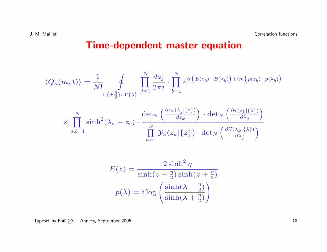
Time-dependent master equation

〈Qκ(m, t)〉 =1

N !

∮Γ±η2∪Γλ

N∏j=1

dzj

2πi·N∏b=1

eit(E(zb)−E(λb)

)+im(p(zb)−p(λb)

)

×N∏

a,b=1

sinh2(λa − zb) ·

detN(∂τκ(λj|z)

∂zk

)· detN

(∂τ(zk|λ)

∂λj

)N∏a=1Yκ(za|z) · detN

(∂Y(λk|λ)

∂λj

)

E(z) =2 sinh2 η

sinh(z − η2) sinh(z + η

2)

p(λ) = i log

(sinh(λ− η

2)

sinh(λ+ η2)

)

– Typeset by FoilTEX – Annecy, September 2005 18

J. M. Maillet Correlation functions

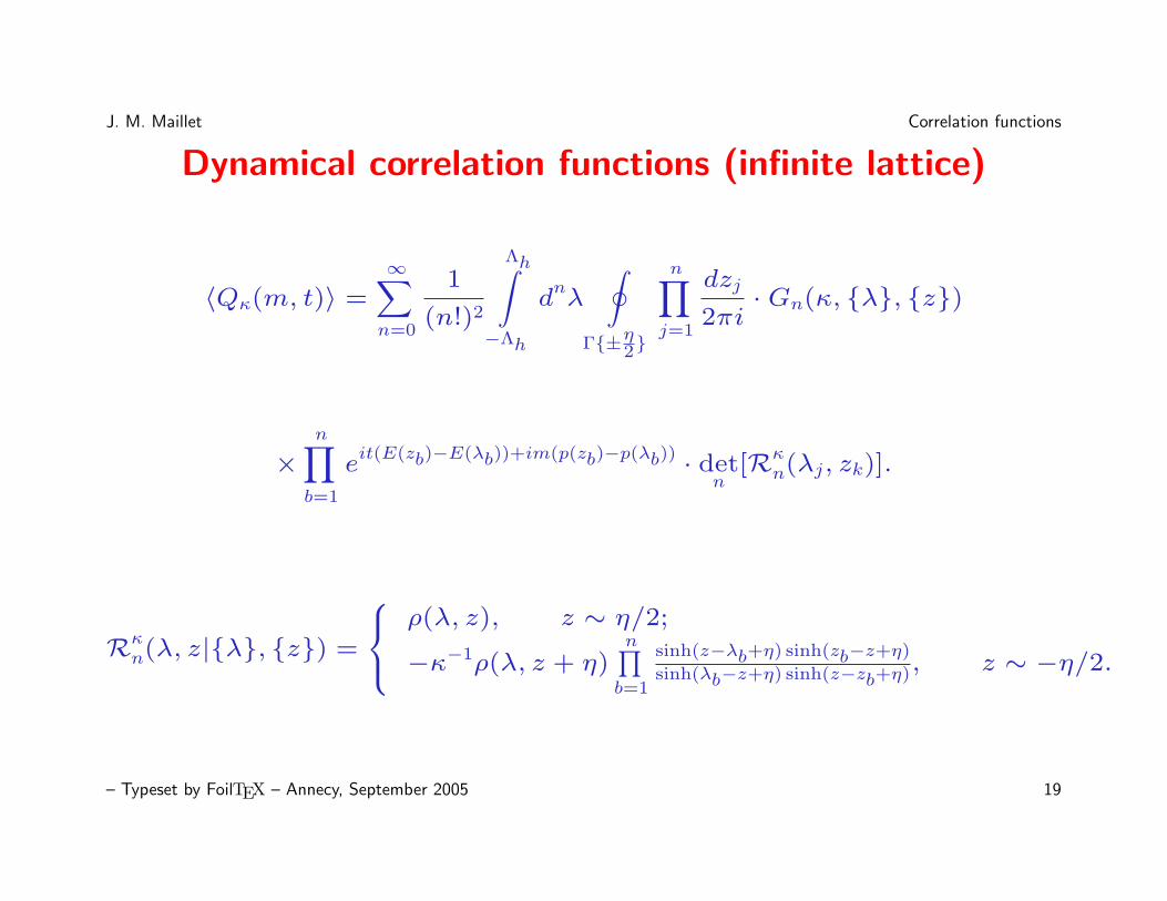
Dynamical correlation functions (infinite lattice)

〈Qκ(m, t)〉 =

∞∑n=0

1

(n!)2

Λh∫−Λh

dnλ

∮Γ±η2

n∏j=1

dzj

2πi·Gn(κ, λ, z)

×n∏b=1

eit(E(zb)−E(λb))+im(p(zb)−p(λb)) · det

n[Rκ

n(λj, zk)].

Rκn(λ, z|λ, z) =

ρ(λ, z), z ∼ η/2;

−κ−1ρ(λ, z + η)n∏b=1

sinh(z−λb+η) sinh(zb−z+η)sinh(λb−z+η) sinh(z−zb+η)

, z ∼ −η/2.

– Typeset by FoilTEX – Annecy, September 2005 19

J. M. Maillet Correlation functions

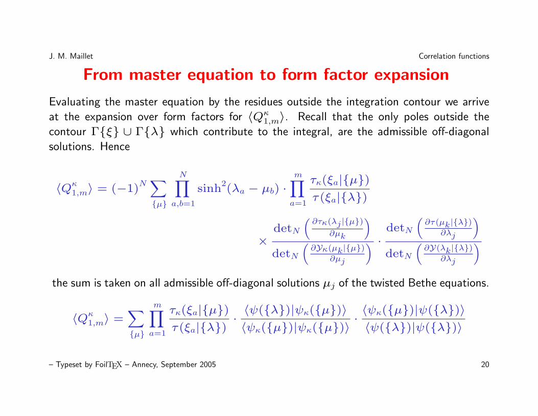
From master equation to form factor expansion

Evaluating the master equation by the residues outside the integration contour we arrive

at the expansion over form factors for 〈Qκ1,m〉. Recall that the only poles outside the

contour Γξ ∪ Γλ which contribute to the integral, are the admissible off-diagonal

solutions. Hence

〈Qκ1,m〉 = (−1)

N∑µ

N∏a,b=1

sinh2(λa − µb) ·

m∏a=1

τκ(ξa|µ)τ(ξa|λ)

×detN

(∂τκ(λj|µ)

∂µk

)detN

(∂Yκ(µk|µ)

∂µj

) · detN(∂τ(µk|λ)

∂λj

)detN

(∂Y(λk|λ)

∂λj

)the sum is taken on all admissible off-diagonal solutions µj of the twisted Bethe equations.

〈Qκ1,m〉 =

∑µ

m∏a=1

τκ(ξa|µ)τ(ξa|λ)

·〈ψ(λ)|ψκ(µ)〉〈ψκ(µ)|ψκ(µ)〉

·〈ψκ(µ)|ψ(λ)〉〈ψ(λ)|ψ(λ)〉

– Typeset by FoilTEX – Annecy, September 2005 20

J. M. Maillet Correlation functions

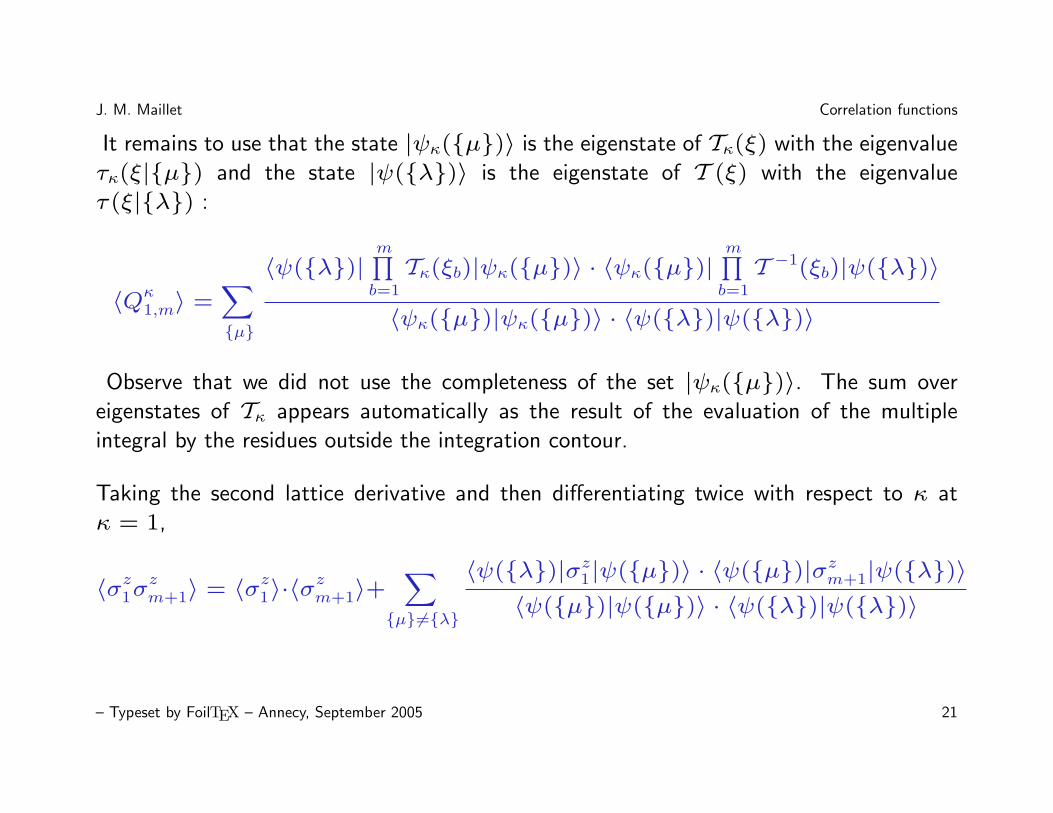
It remains to use that the state |ψκ(µ)〉 is the eigenstate of Tκ(ξ) with the eigenvalue

τκ(ξ|µ) and the state |ψ(λ)〉 is the eigenstate of T (ξ) with the eigenvalue

τ(ξ|λ) :

〈Qκ1,m〉 =

∑µ

〈ψ(λ)|m∏b=1

Tκ(ξb)|ψκ(µ)〉 · 〈ψκ(µ)|m∏b=1

T −1(ξb)|ψ(λ)〉

〈ψκ(µ)|ψκ(µ)〉 · 〈ψ(λ)|ψ(λ)〉

Observe that we did not use the completeness of the set |ψκ(µ)〉. The sum over

eigenstates of Tκ appears automatically as the result of the evaluation of the multiple

integral by the residues outside the integration contour.

Taking the second lattice derivative and then differentiating twice with respect to κ at

κ = 1,

〈σz1σzm+1〉 = 〈σz1〉·〈σ

zm+1〉+

∑µ6=λ

〈ψ(λ)|σz1|ψ(µ)〉 · 〈ψ(µ)|σzm+1|ψ(λ)〉〈ψ(µ)|ψ(µ)〉 · 〈ψ(λ)|ψ(λ)〉

– Typeset by FoilTEX – Annecy, September 2005 21

J. M. Maillet Correlation functions

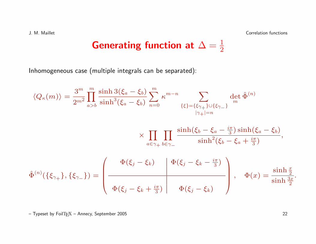
Generating function at ∆ = 12

Inhomogeneous case (multiple integrals can be separated):

〈Qκ(m)〉 =3m

2m2

m∏a>b

sinh 3(ξa − ξb)sinh3(ξa − ξb)

m∑n=0

κm−n ∑

ξ=ξγ+∪ξγ−|γ+|=n

detm

Φ(n)

×∏a∈γ+

∏b∈γ−

sinh(ξb − ξa − iπ3 ) sinh(ξa − ξb)

sinh2(ξb − ξa + iπ3 )

,

Φ(n)

(ξγ+, ξγ−) =

Φ(ξj − ξk) Φ(ξj − ξk − iπ

3 )

Φ(ξj − ξk + iπ3 ) Φ(ξj − ξk)

, Φ(x) =sinh x

2

sinh 3x2

.

– Typeset by FoilTEX – Annecy, September 2005 22

J. M. Maillet Correlation functions

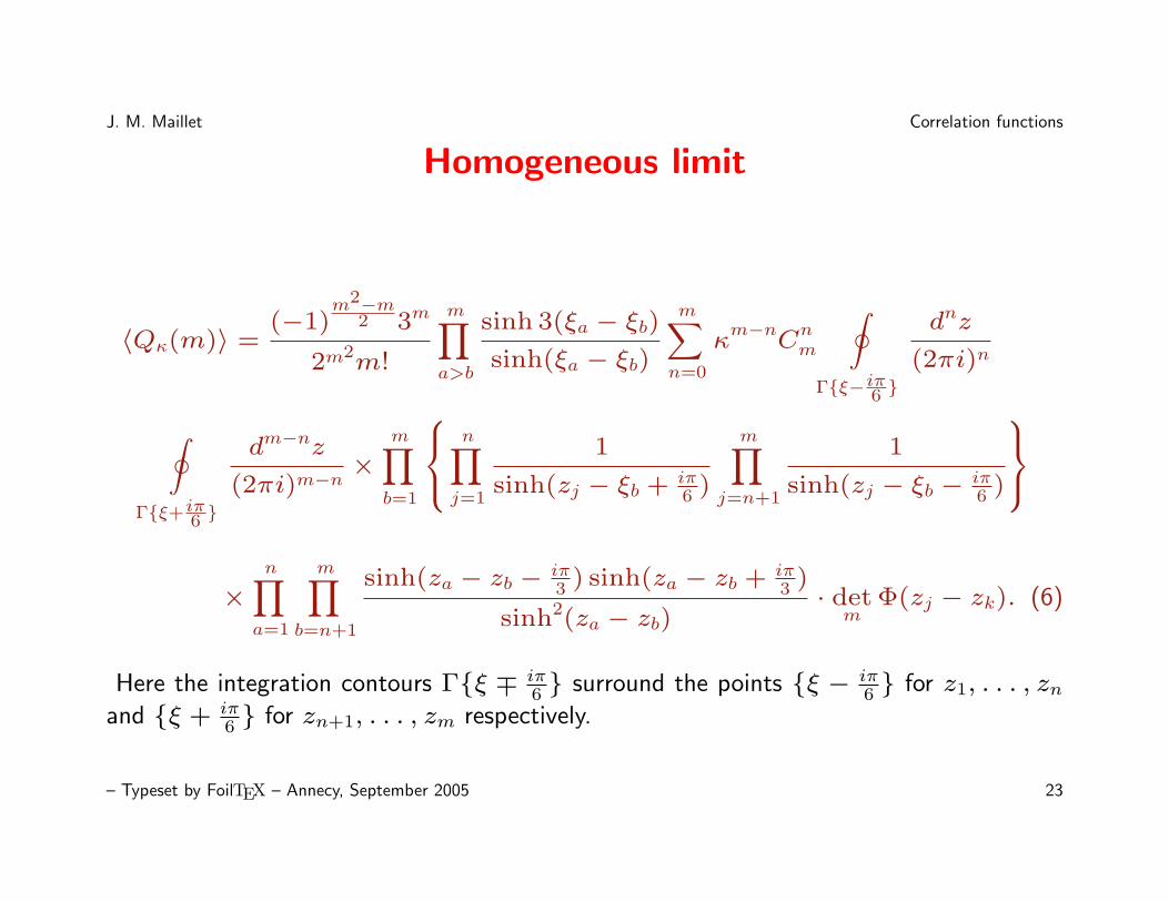
Homogeneous limit

〈Qκ(m)〉 =(−1)

m2−m2 3m

2m2m!

m∏a>b

sinh 3(ξa − ξb)sinh(ξa − ξb)

m∑n=0

κm−n

Cnm

∮Γξ−iπ6

dnz

(2πi)n

∮Γξ+iπ6

dm−nz

(2πi)m−n×

m∏b=1

n∏j=1

1

sinh(zj − ξb + iπ6 )

m∏j=n+1

1

sinh(zj − ξb − iπ6 )

×

n∏a=1

m∏b=n+1

sinh(za − zb − iπ3 ) sinh(za − zb + iπ

3 )

sinh2(za − zb)· detm

Φ(zj − zk). (6)

Here the integration contours Γξ ∓ iπ6 surround the points ξ − iπ

6 for z1, . . . , znand ξ + iπ

6 for zn+1, . . . , zm respectively.

– Typeset by FoilTEX – Annecy, September 2005 23

J. M. Maillet Correlation functions

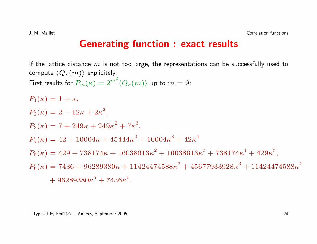
Generating function : exact results

If the lattice distance m is not too large, the representations can be successfully used to

compute 〈Qκ(m)〉 explicitely.

First results for Pm(κ) = 2m2〈Qκ(m)〉 up to m = 9:

P1(κ) = 1 + κ,

P2(κ) = 2 + 12κ+ 2κ2,

P3(κ) = 7 + 249κ+ 249κ2+ 7κ

3,

P4(κ) = 42 + 10004κ+ 45444κ2+ 10004κ

3+ 42κ

4

P5(κ) = 429 + 738174κ+ 16038613κ2+ 16038613κ

3+ 738174κ

4+ 429κ

5,

P6(κ) = 7436 + 96289380κ+ 11424474588κ2+ 45677933928κ

3+ 11424474588κ

4

+ 96289380κ5+ 7436κ

6.

– Typeset by FoilTEX – Annecy, September 2005 24

J. M. Maillet Correlation functions

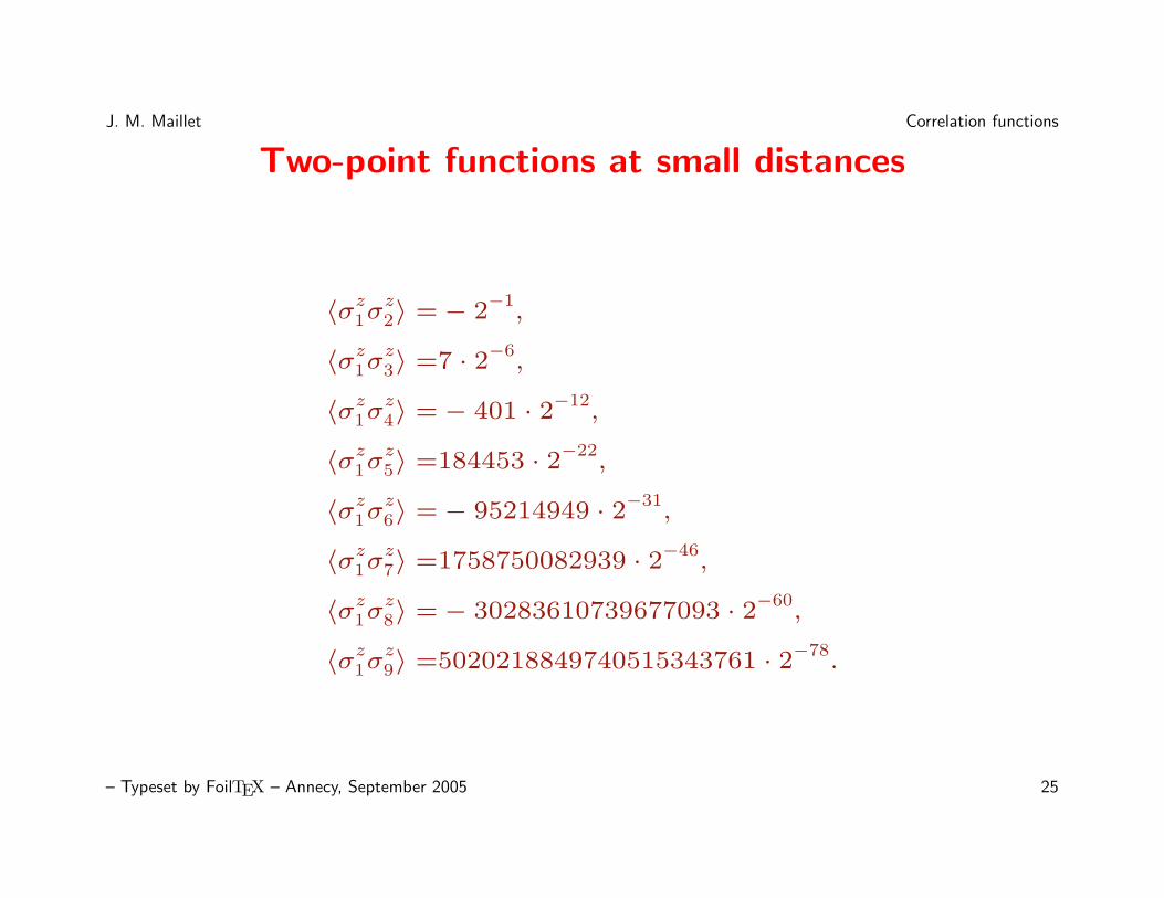
Two-point functions at small distances

〈σz1σz2〉 =− 2

−1,

〈σz1σz3〉 =7 · 2−6

,

〈σz1σz4〉 =− 401 · 2−12

,

〈σz1σz5〉 =184453 · 2−22

,

〈σz1σz6〉 =− 95214949 · 2−31

,

〈σz1σz7〉 =1758750082939 · 2−46

,

〈σz1σz8〉 =− 30283610739677093 · 2−60

,

〈σz1σz9〉 =5020218849740515343761 · 2−78

.

– Typeset by FoilTEX – Annecy, September 2005 25

J. M. Maillet Correlation functions

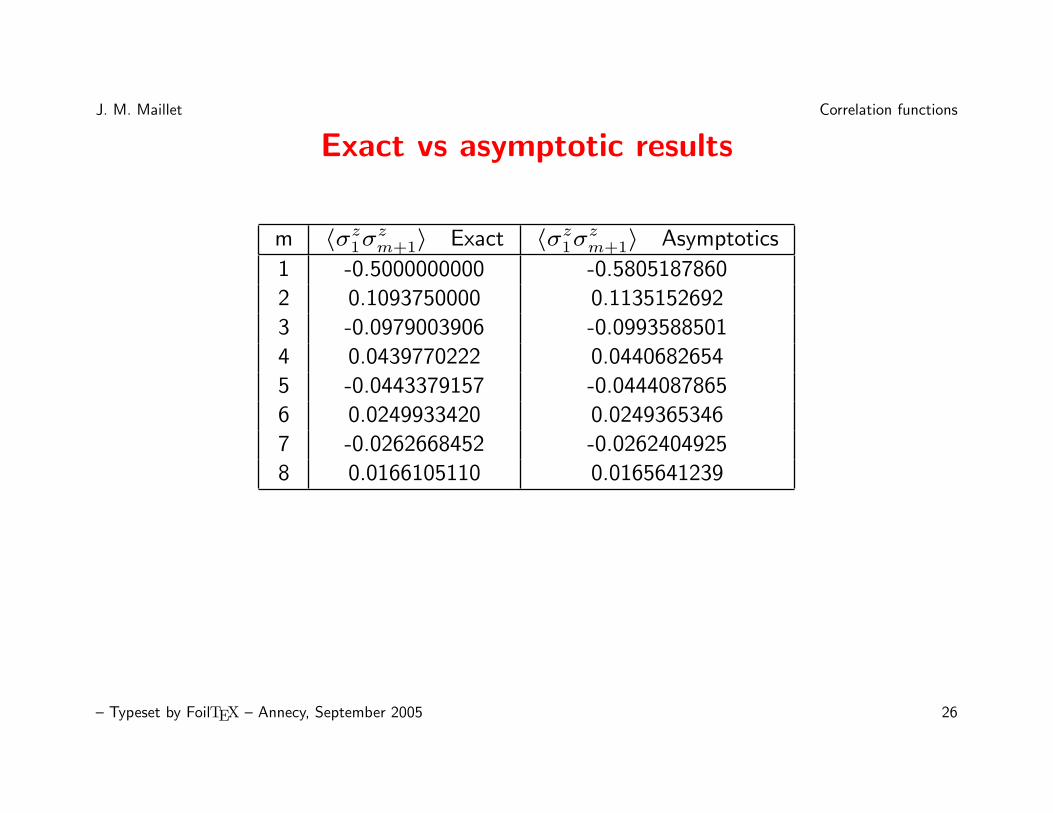
Exact vs asymptotic results

m 〈σz1σzm+1〉 Exact 〈σz1σ

zm+1〉 Asymptotics

1 -0.5000000000 -0.5805187860

2 0.1093750000 0.1135152692

3 -0.0979003906 -0.0993588501

4 0.0439770222 0.0440682654

5 -0.0443379157 -0.0444087865

6 0.0249933420 0.0249365346

7 -0.0262668452 -0.0262404925

8 0.0166105110 0.0165641239

– Typeset by FoilTEX – Annecy, September 2005 26

J. M. Maillet Correlation functions

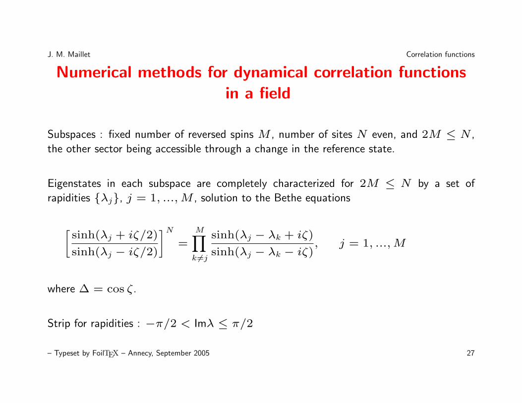
Numerical methods for dynamical correlation functionsin a field

Subspaces : fixed number of reversed spins M , number of sites N even, and 2M ≤ N ,

the other sector being accessible through a change in the reference state.

Eigenstates in each subspace are completely characterized for 2M ≤ N by a set of

rapidities λj, j = 1, ...,M , solution to the Bethe equations

[sinh(λj + iζ/2)

sinh(λj − iζ/2)

]N=

M∏k 6=j

sinh(λj − λk + iζ)

sinh(λj − λk − iζ), j = 1, ...,M

where ∆ = cos ζ.

Strip for rapidities : −π/2 < Imλ ≤ π/2

– Typeset by FoilTEX – Annecy, September 2005 27

J. M. Maillet Correlation functions

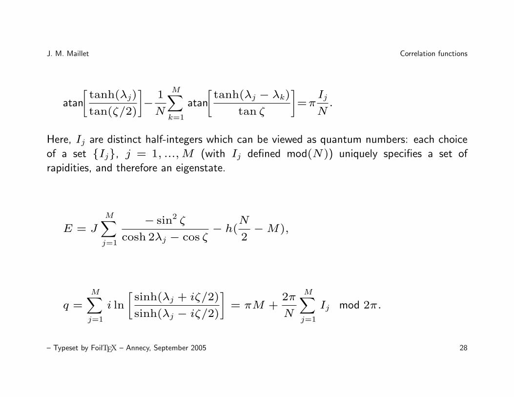
atan

[tanh(λj)

tan(ζ/2)

]−

1

N

M∑k=1

atan

[tanh(λj − λk)

tan ζ

]=π

Ij

N.

Here, Ij are distinct half-integers which can be viewed as quantum numbers: each choice

of a set Ij, j = 1, ...,M (with Ij defined mod(N)) uniquely specifies a set of

rapidities, and therefore an eigenstate.

E = J

M∑j=1

− sin2 ζ

cosh 2λj − cos ζ− h(

N

2−M),

q =M∑j=1

i ln

[sinh(λj + iζ/2)

sinh(λj − iζ/2)

]= πM +

2π

N

M∑j=1

Ij mod 2π.

– Typeset by FoilTEX – Annecy, September 2005 28

J. M. Maillet Correlation functions

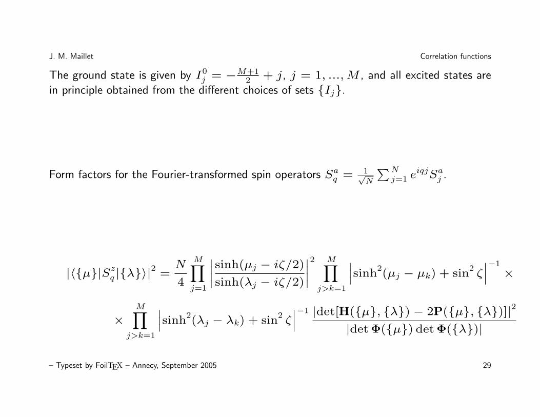
The ground state is given by I0j = −M+1

2 + j, j = 1, ...,M , and all excited states are

in principle obtained from the different choices of sets Ij.

Form factors for the Fourier-transformed spin operators Saq = 1√N

∑Nj=1 e

iqjSaj .

|〈µ|Szq |λ〉|2=N

4

M∏j=1

∣∣∣∣sinh(µj − iζ/2)sinh(λj − iζ/2)

∣∣∣∣2 M∏j>k=1

∣∣∣sinh2(µj − µk) + sin

2ζ∣∣∣−1

×

×M∏

j>k=1

∣∣∣sinh2(λj − λk) + sin

2ζ∣∣∣−1 |det[H(µ, λ)− 2P(µ, λ)]|2

|det Φ(µ) det Φ(λ)|

– Typeset by FoilTEX – Annecy, September 2005 29

J. M. Maillet Correlation functions

Hab(µ, λ) =1

sinh(µa − λb)

M∏j 6=a

sinh(µj − λb − iζ)−

[sinh(λb + iζ/2)

sinh(λb − iζ/2)

]N M∏j 6=a

sinh(µj − λb + iζ)

Pab(µ, λ) =1

sinh2 µa + sin2 ζ/2

M∏k=1

sinh(λk − λb − iζ),

Structure factor :

Saa

(q, ω) = 2π∑α6=GS

|〈GS|Saq |α〉|2δ(ω − ωα)

– Typeset by FoilTEX – Annecy, September 2005 30

J. M. Maillet Correlation functions

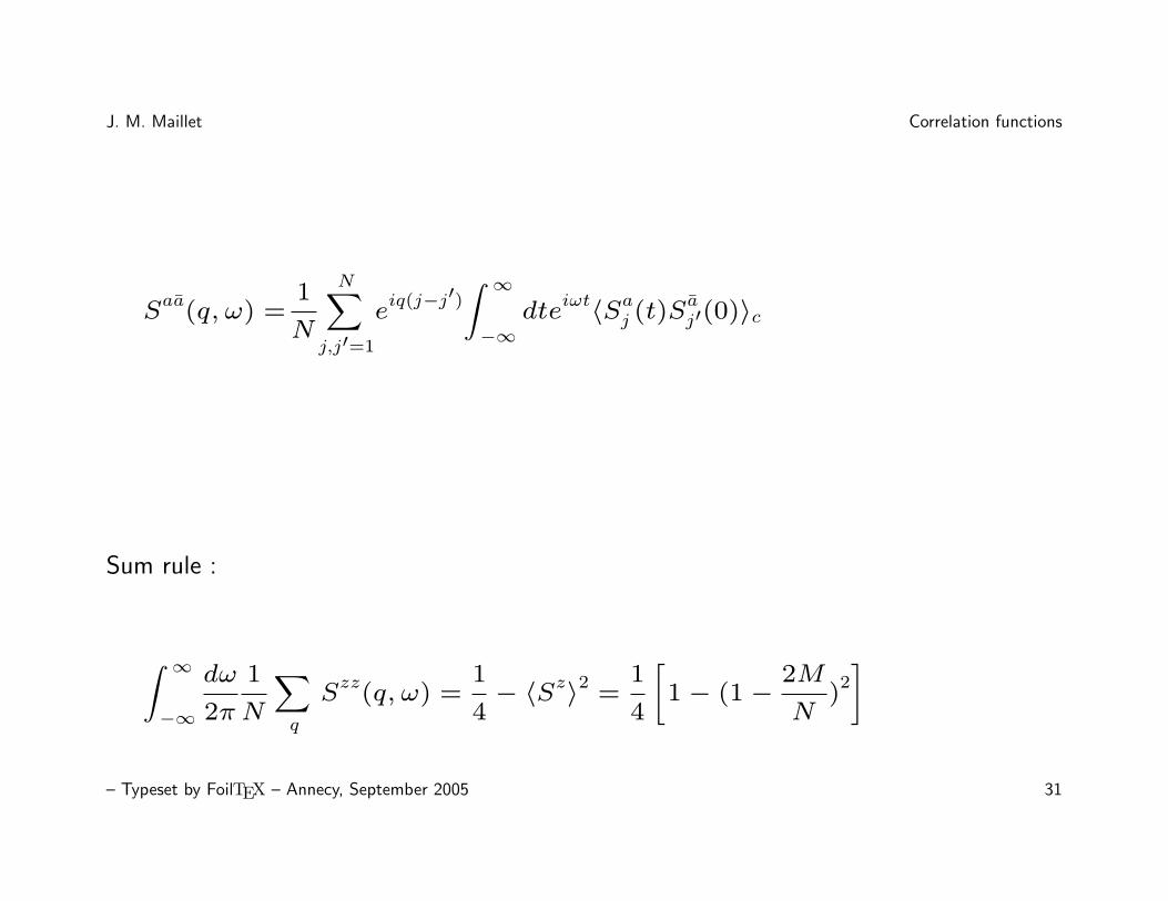
Saa

(q, ω) =1

N

N∑j,j′=1

eiq(j−j′)

∫ ∞−∞

dteiωt〈Saj (t)S

aj′(0)〉c

Sum rule :

∫ ∞−∞

dω

2π

1

N

∑q

Szz

(q, ω) =1

4− 〈Sz〉2 =

1

4

[1− (1−

2M

N)2

]

– Typeset by FoilTEX – Annecy, September 2005 31

J. M. Maillet Correlation functions

Table 1: Comparison of equal-time correlation functions 〈Saj Saj+l〉 at zerofield for ∆ = 0.25 for small distances l = 1, 2, 3. Subscript p refers to theexact polynomial representation, whereas ff refers to our results obtainedby summing form factors for all states up to three holes, thereby achievingsaturation of the sum rule to 99.88 % (Szz) and 95.61 % (S−+).

l Szzp Szzff S−+p S−+

ff

1 -0.113489 -0.113337 -0.316807 -0.311455

2 0.0129789 0.0129605 0.180965 0.180967

3 -0.0163964 -0.0163965 -0.152364 -0.152466

– Typeset by FoilTEX – Annecy, September 2005 32

J. M. Maillet Correlation functions

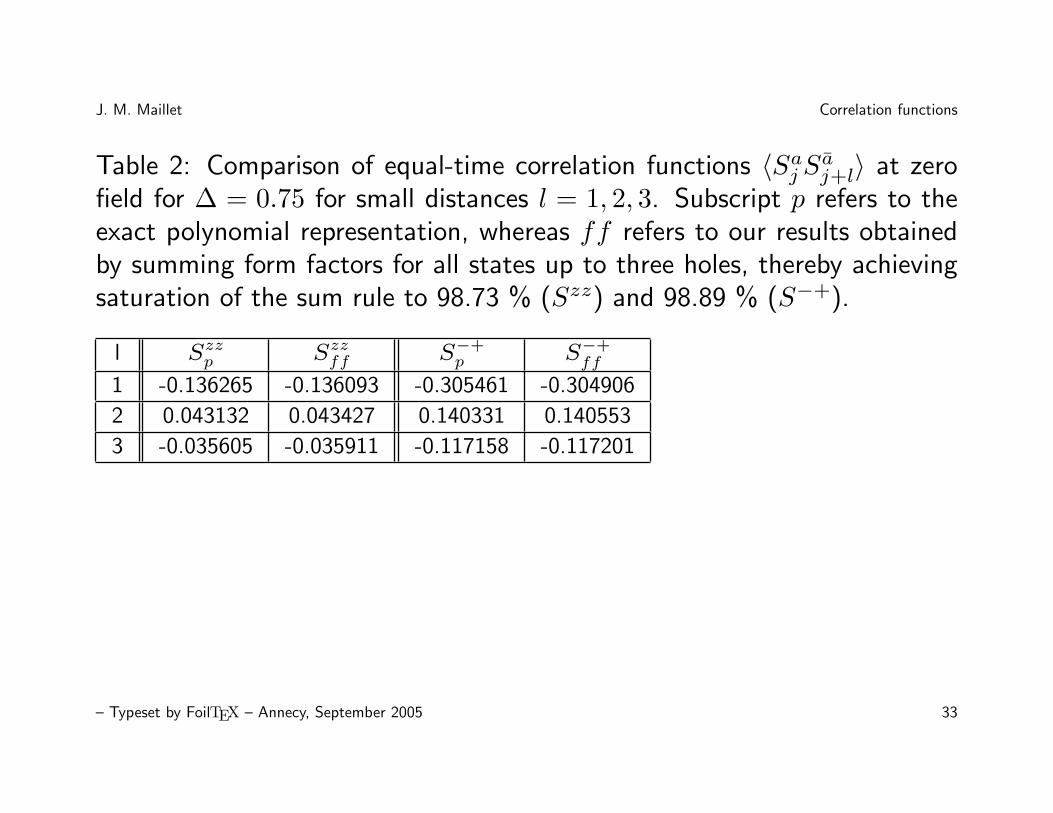
Table 2: Comparison of equal-time correlation functions 〈Saj Saj+l〉 at zerofield for ∆ = 0.75 for small distances l = 1, 2, 3. Subscript p refers to theexact polynomial representation, whereas ff refers to our results obtainedby summing form factors for all states up to three holes, thereby achievingsaturation of the sum rule to 98.73 % (Szz) and 98.89 % (S−+).

l Szzp Szzff S−+p S−+

ff

1 -0.136265 -0.136093 -0.305461 -0.304906

2 0.043132 0.043427 0.140331 0.140553

3 -0.035605 -0.035911 -0.117158 -0.117201

– Typeset by FoilTEX – Annecy, September 2005 33

J. M. Maillet Correlation functions

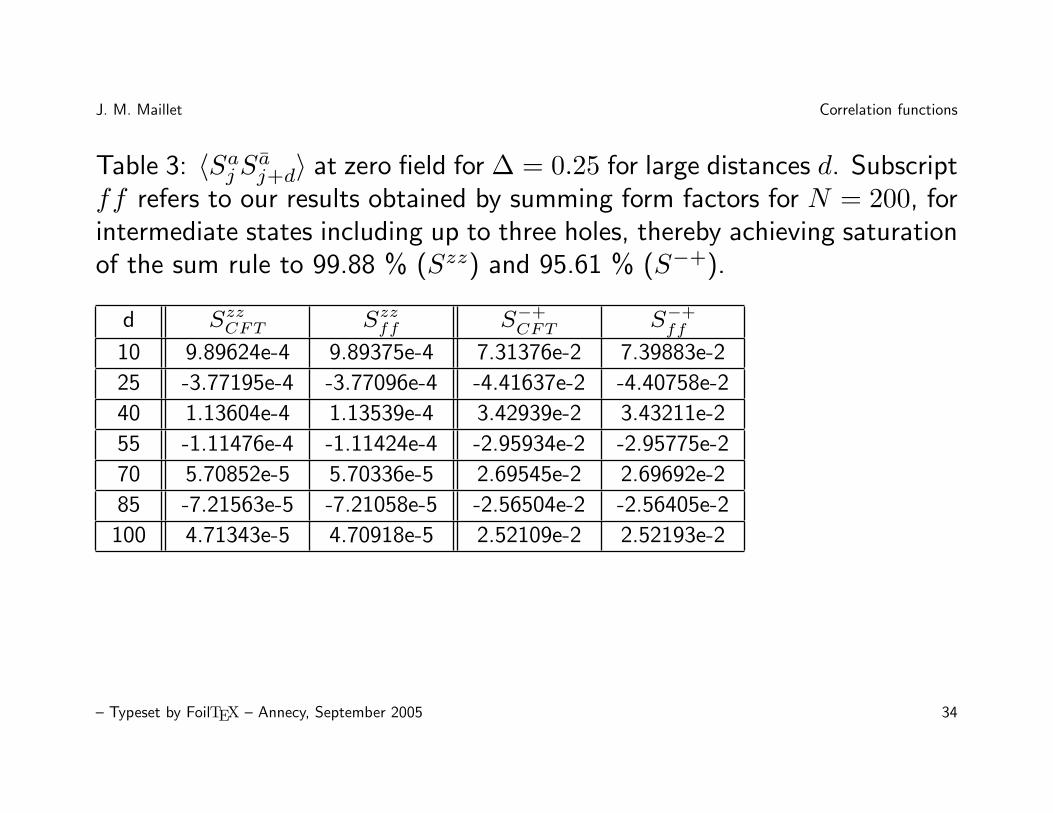
Table 3: 〈Saj Saj+d〉 at zero field for ∆ = 0.25 for large distances d. Subscriptff refers to our results obtained by summing form factors for N = 200, forintermediate states including up to three holes, thereby achieving saturationof the sum rule to 99.88 % (Szz) and 95.61 % (S−+).

d SzzCFT Szzff S−+CFT S−+

ff

10 9.89624e-4 9.89375e-4 7.31376e-2 7.39883e-2

25 -3.77195e-4 -3.77096e-4 -4.41637e-2 -4.40758e-2

40 1.13604e-4 1.13539e-4 3.42939e-2 3.43211e-2

55 -1.11476e-4 -1.11424e-4 -2.95934e-2 -2.95775e-2

70 5.70852e-5 5.70336e-5 2.69545e-2 2.69692e-2

85 -7.21563e-5 -7.21058e-5 -2.56504e-2 -2.56405e-2

100 4.71343e-5 4.70918e-5 2.52109e-2 2.52193e-2

– Typeset by FoilTEX – Annecy, September 2005 34

J. M. Maillet Correlation functions

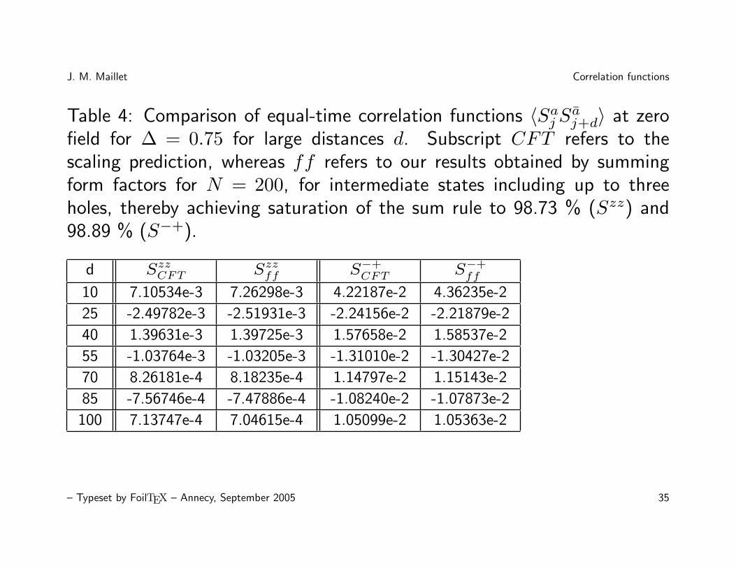
Table 4: Comparison of equal-time correlation functions 〈Saj Saj+d〉 at zerofield for ∆ = 0.75 for large distances d. Subscript CFT refers to thescaling prediction, whereas ff refers to our results obtained by summingform factors for N = 200, for intermediate states including up to threeholes, thereby achieving saturation of the sum rule to 98.73 % (Szz) and98.89 % (S−+).

d SzzCFT Szzff S−+CFT S−+

ff

10 7.10534e-3 7.26298e-3 4.22187e-2 4.36235e-2

25 -2.49782e-3 -2.51931e-3 -2.24156e-2 -2.21879e-2

40 1.39631e-3 1.39725e-3 1.57658e-2 1.58537e-2

55 -1.03764e-3 -1.03205e-3 -1.31010e-2 -1.30427e-2

70 8.26181e-4 8.18235e-4 1.14797e-2 1.15143e-2

85 -7.56746e-4 -7.47886e-4 -1.08240e-2 -1.07873e-2

100 7.13747e-4 7.04615e-4 1.05099e-2 1.05363e-2

– Typeset by FoilTEX – Annecy, September 2005 35

J. M. Maillet Correlation functions

Conclusions and Perspectives

New method to obtain correlation functions of quantum integrable models

• Generic tools for a large class of models

• Explicit results for the Heisenberg spin chains

Open new perspectives

• Asymptotic behavior of correlation functions (under study)

• Dynamical correlation functions and depending on temperature

• Applications to many different models (models with impurities, with boundaries, field

theories,...)

• Numerical evaluations via form factor expansion

– Typeset by FoilTEX – Annecy, September 2005 36